On the Acceleration of Deep Learning Model Parallelism with Staleness

Abstract

Training the deep convolutional neural network for computer vision problems is slow and inefficient, especially when it is large and distributed across multiple devices. The inefficiency is caused by the backpropagation algorithm’s forward locking, backward locking, and update locking problems. Existing solutions for acceleration either can only handle one locking problem or lead to severe accuracy loss or memory inefficiency. Moreover, none of them consider the straggler problem among devices. In this paper, we propose Layer-wise Staleness and a novel efficient training algorithm, Diversely Stale Parameters (DSP), to address these challenges. We also analyze the convergence of DSP with two popular gradient-based methods and prove that both of them are guaranteed to converge to critical points for non-convex problems. Finally, extensive experimental results on training deep learning models demonstrate that our proposed DSP algorithm can achieve significant training speedup with stronger robustness than compared methods.

1 Introduction

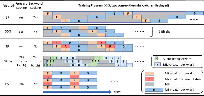
Figure 1: Sketches of different methods with three blocks. The forward and recomputation are overlapped in DSP.

The deep convolutional neural network is an important method for solving computer vision problems such as classification, object detection, etc. However, as the neural networks get deeper and larger [8, 17, 10, 32, 35, 24], the required expensive training time has become the bottleneck. Data parallelism [34, 23, 3] and model parallelism [22, 20] are two standard parallelism techniques to utilize multiple devices for efficient training.

The data parallelism for efficient distributed training has been well studied and implemented in existing libraries [1, 4, 12, 36, 14, 16], but the model parallelism is still underexplored. In this paper, we focus on the model parallelism, where the deep neural network (DNN) benefits from being split onto multiple devices. But the resource utilization of standard model parallelism can be very low. The backpropagation algorithm [30, 21] typically requires two phases to update the model in each training step: the forward pass and backward pass. But the sequential propagation of activation and error gradient leads to backward locking and forward locking [18] respectively because of the computation dependencies between layers. The update locking [18] exists as the backward pass will not start until the forward pass has completed. This sequential execution keeps a device inefficiently waiting for the activation input and error gradient.

Several works have been proposed to address these locking issues (Figure 1). [18] uses Decoupled Neural Interfaces (DNI) to predict the error gradient via auxiliary networks, so that a layer uses the synthetic gradient and needs not to wait for the error gradient. [28] lets hidden layers receive error information directly from the output layer. However, these methods can not converge when dealing with very deep neural networks. [2] proposes layer-wise decoupled greedy learning (DGL), which introduces an auxiliary classifier for each block of layers so that a block updates its parameters according to its own classifier. But the objective function of DGL based on greedy local predictions can be very different from the original model. GPipe [11] proposes pipeline parallelism and divides each mini-batch into micro-batches, which can be regarded as a combination of model parallelism and data parallelism. However, the forward and backward lockings of the micro-batch still exist, and the update locking is not addressed because GPipe waits for the whole forward and backward pass to finish before updating the parameters. [15] proposes Decoupled Parallel Backpropagation (DDG), which divides the DNN into blocks and removes the backward locking by storing delayed error gradient and intermediate activations at each block. But DDG suffers from large memory consumption due to storing all the intermediate results. PipeDream [26] has to store multiple versions of weights in addition to intermediate activations as in DDG. Features Replay (FR) [13, 37] improves DDG via storing the history inputs and recomputing the intermediate results. Nevertheless, blocks in DDG and FR still need to wait for the backward error gradient. Besides, neither DDG nor FR addresses the forward locking problem.

To overcome the aforementioned drawbacks, we first propose Layer-wise Staleness, a fine-grained staleness within the model to allow different parts to be trained independently. Incorporating staleness is useful for efficient asynchronous execution without synchronization barrier [9], which can be interpreted as another form of locking/dependency. The introduction of preset Layer-wise Staleness enables each part of the convolutional neural network (CNN) to run in a very flexible way with a certain degree of asynchrony. Based on the concept of Layer-wise Staleness, we propose a novel parallel CNN training algorithm named as Diversely Stale Parameters (DSP), where lower layers use more stale information to update parameters. DSP also utilizes the recomputation technique [5, 7] to reduce memory consumption, which is overlapped with the forward pass. Our contributions are summarized as follows:

• We propose Layer-wise Staleness and Diversely Stale Parameters (§3) which breaks the forward, backward and update lockings without memory issues.

• To ensure the theoretical guarantee, we provide convergence analysis (§4) for the proposed method. Even faced with parameters of different Layer-wise Staleness, we prove that DSP converges to critical points for non-convex problems with SGD and momentum SGD.

• We evaluate our method via training deep convolutional neural networks (§5). Extensive empirical results show that DSP achieves significant training speedup and strong robustness against random stragglers.

2 Background

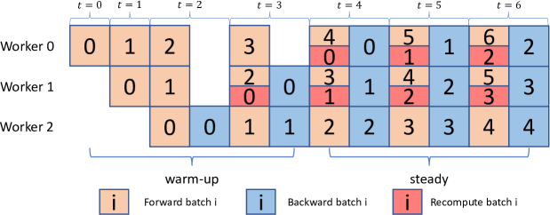
Figure 2: DSP(1,1,0;4,2,0) with Layer-wise Staleness of {4,2,0} (the index difference between the forward and backward batch). Worker $k\in\{0,1,2\}$ holds block $k$.

We divide a CNN into $K$ consecutive blocks so that the whole parameters $x=\left(x_{0},x_{1},...,x_{K-1}\right)\in\mathbb{R}^{d}$, where $x_{k}\in\mathbb{R}^{d_{k}}$ denotes the partial parameters at block $k\in\{0,1,...,K-1\}$ and $d=\sum^{K-1}_{k=0}d_{k}$. Each block $k$ computes activation $h_{k+1}=f_{k}(h_{k};x_{k})$, where $h_{k}$ denotes the input of block $k$. In particular, $h_{0}$ is the input data. For simplicity, we define $F(h_{0};x_{0};x_{1};...;x_{k})\coloneqq f_{k}(...f_{1}(f_{0}(h_{0};x_{0});x_{1})...;x_{k})=h_{k+1}$. The loss is $\mathcal{L}(h_{K},l)$, where $l$ is the label. Minimizing the loss of a $K$-block neural network can be represented by the following problem:

$$\min_{x\in\mathbb{R}^{d}}\quad f(x)\coloneqq\mathcal{L}(F(h_{0};x_{0};x_{1};...;x_{K-1}),l).$$ (1)

Backpropagation algorithm computes the gradient for block $k$ following chain rule via Eq. (2). The forward locking exists because the input of each block is dependent on the output from the lower block. The backward locking exists because each block cannot compute gradients until having received the error gradient $\mathcal{G}_{h}$ from the upper block. Besides, the backward process can not start until the whole forward process is completed, which is known as the update locking.

$$\begin{cases}\mathcal{G}_{h_{k}}=\frac{\partial f_{k}(h_{k};x_{k})}{\partial h_{k}}\mathcal{G}_{h_{k+1}},\quad\mathcal{G}_{h_{K}}=\frac{\partial\mathcal{L}(h_{K},l)}{\partial h_{K}}\\ \mathcal{G}_{x_{k}}=\frac{\partial f_{k}(h_{k};x_{k})}{\partial x_{k}}\mathcal{G}_{h_{k+1}}.\end{cases}$$ (2)

After computing the gradients, stochastic gradient descent (SGD) [29] and its variants such as stochastic unified momentum (SUM) [38], RMSPROP [33] and ADAM [19] are widely used for updating the model. SGD updates via $x^{n+1}=x^{n}-\alpha\mathcal{G}(x^{n};\xi)$, where $x^{n}$ is the parameters when feeding the $n^{\text{th}}$ data (batch), $\alpha$ is the learning rate, and $\mathcal{G}(x^{n};\xi)$ is the stochastic gradient. SUM updates the parameters via Eq. (3), where $\beta$ is the momentum constant and $y$ is the momentum term. When $s=1$, SUM reduces to stochastic Nesterov’s accelerated gradient (SNAG) [27].

$$\begin{cases}y^{n+1}=x^{n}-\alpha\mathcal{G}(x^{n};\xi),\,\,y^{s,n+1}=x^{n}-s\alpha\mathcal{G}(x^{n};\xi)\\ x^{n+1}=y^{n+1}+\beta(y^{s,n+1}-y^{s,n}).\end{cases}$$ (3)

3 Diversely Stale Parameters

In this section, we propose a novel training method named Diversely Stale Parameters (Figure 2). We first define layer-wise staleness and related notations in Section 3.1, then the motivation and formulation of DSP gradient in Section 3.2, finally the practical implementation using queues for pipelined batch input in Section 3.3.

3.1 Layer-Wise Staleness

Let the data be forwarded with parameters $x_{0}$ at timestamp $t_{0}$, $x_{1}$ at timestamp $t_{1}$, $\ldots$, and $x_{K-1}$ at timestamp $t_{K-1}$. For simplicity we denote the Forward Parameters as $\{x_{k}^{t_{k}}\}_{k=0,\ldots,K-1}$. Similarly we denote the Backward Parameters as $\{x_{k}^{t_{2K-1-k}}\}_{k=0,\ldots,K-1}$. Then we define Layer-wise Staleness as $\Delta t_{k}=t_{2K-k-1}-t_{k}\geq 0$. We preset each block’s Layer-wise Staleness to a different value to break the synchronization barrier of backpropagation.

We also denote the maximum Layer-wise Staleness as $\Delta t=\max_{k=0,1,\ldots,K-1}\Delta t_{k}$. It is worth noting that a) in standard backpropagation algorithm (Eq. (2)), Layer-wise Staleness $\Delta t_{k}=0$; and b) Feeding data index is not identical to timestamp/training step.

3.2 DSP Gradient

We first set the constraints of DSP as $t_{0}<t_{1}<\ldots<t_{K-1}\leq t_{K}<t_{K+1}<\ldots<t_{2K-1}$ such that both the dependencies in the forward and backward pass no longer exist, because we do not need them to finish in the same timestamp anymore. The non-decreasing property corresponds to the fact that the data needs to go through the bottom layers before the top layers, and the error gradient needs to go through the top layers before the bottom layers.

Based on backpropagation algorithm and Eq. (2), we should compute the gradients according to the following formulas as we are updating the Backward Parameters $\{x_{k}^{t_{2K-1-k}}\}_{k=0,\ldots,K-1}$,

$$\begin{split}&\mathcal{G}_{x_{k}}=\frac{\partial F(h_{0};x^{t_{2K-1}}_{0};...;x^{t_{2K-1-k}}_{k})}{\partial x^{t_{2K-1-k}}_{k}}\mathcal{G}_{h_{k+1}}\\ &\mathcal{G}_{h_{k}}=\frac{\partial F(h_{0};x^{t_{2K-1}}_{0};...;x^{t_{2K-1-k}}_{k})}{\partial F(h_{0};x^{t_{2K-1}}_{0};...;x^{t_{2K-2-k}}_{k-1})}\mathcal{G}_{h_{k+1}}\\ &\mathcal{G}_{h_{K}}=\frac{\partial\mathcal{L}(F(h_{0};x^{t_{2K-1}}_{0};...;x^{t_{K}}_{K-1}),l)}{F(h_{0};x^{t_{2K-1}}_{0};...;x^{t_{K}}_{K-1})}\,.\end{split}$$ (4)

However, during the forward pass the input of block $k$ is $F(h_{0};x_{0}^{t_{0}};...;x_{k-1}^{t_{k-1}})$. Therefore we incorporate the recomputation technique and utilize both the Forward Parameters and Backward Parameters to compute DSP gradient as follows,

$$\begin{split}&\mathcal{G}_{x_{k}}=\frac{\partial F(h_{0};x^{t_{0}}_{0};...;x^{t_{k-1}}_{k-1};\bm{x^{t_{2K-1-k}}_{k}})}{\partial\bm{x^{t_{2K-1-k}}_{k}}}\mathcal{G}_{h_{k+1}}\\ &\mathcal{G}_{h_{k}}=\frac{\partial F(h_{0};x^{t_{0}}_{0};...;x^{t_{k-1}}_{k-1};\bm{x^{t_{2K-1-k}}_{k}})}{\partial F(h_{0};x^{t_{0}}_{0};...;x^{t_{k-1}}_{k-1})}\mathcal{G}_{h_{k+1}}\\ &\mathcal{G}_{h_{K}}=\frac{\partial\mathcal{L}(F(h_{0};x^{t_{0}}_{0};...;x^{t_{K-1}}_{K-1}),l)}{F(h_{0};x^{t_{0}}_{0};...;x^{t_{K-1}}_{K-1})}.\end{split}$$ (5)

The intuition behind the DSP gradient of Eq. (5) is that it is equivalent to Eq. (4) when the model converges to a local optimum where the gradient is zero ($x_{k}^{t_{k}}=x_{k}^{t_{2K-1-k}}$ afterwards).

3.3 Batch Pipeline Input

The computation of the DSP gradient breaks the forward and backward dependencies/lockings of the same data as it will not appear in different blocks at the same timestamp. The update locking is naturally broken.

For the parallel implementation of DSP as shown in Figure 2, we incorporate the data batch pipeline to keep all the blocks being fed with different data batches and running. The data source consecutively feeds data input. Different blocks transport and process different data via FIFO queues. As a result, the data travels each block at different timestamps. Specifically, each block $k$ maintains an input queue $\mathcal{M}_{k}$, output queue $\mathcal{P}_{k}$ and gradient queue $\mathcal{Q}_{k}$ of length $1+m_{k}$, $1+p_{k}$ and $1+q_{k}$ respectively. We denote it as $DSP(p_{0},...,p_{K-1};m_{0},...,m_{K-1})$. $\{q_{k}\}$ is determined by $\{p_{k}\}$ and $\{m_{k}\}$ because the input should match the corresponding error gradient. We manually split the model to different workers to balance the workload at the steady stage.

Apart from adopting recomputation to reduce memory consumption, DSP overlaps recomputation with the forward pass to save time. Using queues also make DSP overlap the communication between blocks with computation. The FIFO queues allow for some asynchrony which is effective for dealing with random stragglers. The ideal time complexity of DSP is $\mathcal{O}(\frac{T_{F}+T_{B}}{K})$ and the space complexity is $\mathcal{O}(L+\sum^{K-1}_{k=0}(m_{k}+p_{k}+q_{k}))$, where $T_{F}$ and $T_{B}$ are serial forward and backward time, and $L$ is the number of layers. $m_{k}$ also represents the Layer-wise Staleness $\Delta t_{k}$ of block $k$. $K$ and the FIFO queues length $m_{k}+1,p_{k}+1,q_{k}+1\ll L$ for deep models, so the extra space cost is trivial.

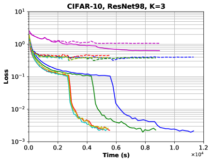
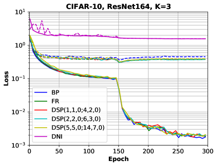
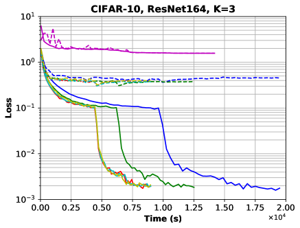
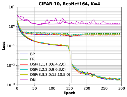
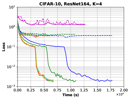
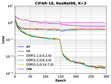
Figure 3: Training loss (solid line) and testing loss (dash line) for ResNet98, ResNet164 on CIFAR-10. The first row and second row plots the loss regarding the training epochs and time respectively.

Table 1: Best Top-1 Test Accuracy

		ResNet164		ResNet98
		CIFAR-10	CIFAR-100	CIFAR-10	CIFAR-100
	BP	94.41%	75.66%	93.38%	72.66%
K=3	FR	94.55%	76.25%	93.60%	73.27%
	DSP(1,1,0;4,2,0)	94.68%	76.05%	93.36%	72.99%
	DSP(2,2,0;6,3,0)	93.98%	76.00%	93.68%	73.70%
	DSP(3,3,0;10,5,0)	93.37%	76.29%	93.27%	73.38%
K=4	FR	94.44%	75.84%	93.26%	72.41%
	DSP(1,1,1,0;6,4,2,0)	94.32%	76.22%	93.41%	73.14%
	DSP(2,2,2,0;9,6,3,0)	94.87%	75.59%	93.06%	72.89%
	DSP(3,3,3,0;15,10,5,0)	93.34%	75.15%	93.45%	72.96%

4 Convergence Analysis

The convergence of DSP with SGD is first analyzed, then DSP with Momentum SGD. For simplicity, we denote the Forward and Backward Parameters of data $n$ as $x^{n^{\prime}}$ and $x^{n}$ respectively.

Assumption 1.

(Bounded variance) Assume that the DSP stochastic gradient $\mathcal{G}(x;\xi)$ satisfies $\text{Var}\left[\mathcal{G}(x;\xi)\right]\leq\sigma^{2}$. Note $\mathbb{E}\left[\mathcal{G}(x;\xi)\right]=\mathcal{G}(x)\neq\nabla f(x)$.

Assumption 2.

(Lipschitz continuous gradient) Assume that the loss and the output of the blocks have Lipschitz continuous gradient, that is, $\forall k\in\{0,1,..,K-1\}$, and $\forall(x_{0,1},...,x_{k,1}),(x_{0,2},...,x_{k,2})\in\mathbb{R}^{d_{0}+d_{1}+...+d_{k}}$, we have $\left\|\nabla F\left(h_{0};x_{0,1};...;x_{k,1}\right)-\nabla F(h_{0};x_{0,2};...;x_{k,2})\right\|\leq L_{k}\left\|(x_{0,1},...,x_{k,1})-(x_{0,2},...,x_{k,2})\right\|$; and $\forall x_{1}$, $x_{2}\in\mathbb{R}^{d}$, $\left\|\nabla f(x_{1})-\nabla f(x_{2})\right\|\leq L_{K}\left\|x_{1}-x_{2}\right\|$.

We define $L\coloneqq\max_{k\in\{0,1,...,K\}}L_{k}$. Note that $\nabla F\left(h_{0};x_{0,1};...;x_{k,1}\right)$ and $\nabla F(h_{0};x_{0,2};...;x_{k,2})$ regarding parameters are Jacobian matrices. In fact, this is assuming that the partial model consisted of the blocks that the data has traveled, has Lipschitz continuous gradient.

Assumption 3.

(Bounded error gradient) Assume that the norm of the error gradient that a block receives is bounded, that is, for any $x\in\mathbb{R}^{d}$, $\forall k\in\{0,1,...,K-2\}$, we have $\left\|\frac{\partial f_{k+1}(h_{k+1};x_{k+1})}{\partial h_{k+1}}...\frac{\partial f_{K-1}(h_{K-1};x_{K-1})}{\partial h_{K-1}}\frac{\partial\mathcal{L}(h_{K},l)}{\partial h_{K}}\right\|\leq M\quad\text{and}\quad\left\|\frac{\partial\mathcal{L}(h_{K},l)}{\partial h_{K}}\right\|\leq M$.

This is assuming that the error gradient at each block does not explode. It is natural to make the above two block-wise assumptions as we are breaking the neural networks into blocks.

Lemma 1.

If Assumptions 2 and 3 hold, the difference between DSP gradient and BP gradient regarding the parameters of block $k\in\{0,1,...,K-1\}$ satisfies $\|\nabla_{x_{k}}\mathcal{L}(F(h_{0};x^{t_{0}}_{0};...;x^{t_{K-1}}_{K-1}),y)-\mathcal{G}_{x_{k}}(x^{t_{2K-1}}_{0};...;x^{t_{K}}_{K-1})\|\leq LM\sum^{K-1}_{i=k}\left\|x^{t_{2K-1-i}}_{i}-x^{t_{i}}_{i}\right\|$.

4.1 DSP with SGD

Theorem 1.

Assume Assumptions 1, 2 and 3 hold. Let $c_{0}=M^{2}K(K+1)^{2}$, and $c_{1}=-(\Delta t^{2}+2)+\sqrt{(\Delta t^{2}+2)^{2}+2c_{0}\Delta t^{2}}$. If the learning rate $\alpha_{n}\leq\frac{c_{1}}{Lc_{0}\Delta t^{2}}$, then $\frac{\sum^{N-1}_{n=0}\alpha_{n}\mathbb{E}\left\|\nabla f(x^{n^{\prime}})\right\|^{2}}{\sum^{N-1}_{n=0}\alpha_{n}}\leq\frac{2\left[f(x^{0})-f^{*}\right]}{\sum^{N-1}_{n=0}\alpha_{n}}+\frac{L\sigma^{2}(2+K\Delta t^{2}+\frac{1}{4}Kc_{1})\sum^{N-1}_{n=0}\alpha_{n}^{2}}{\sum^{N-1}_{n=0}\alpha_{n}}$.

Corollary 1.

(Sublinear convergence rate) According to Theorem 1, by setting the learning rate $\alpha_{n}=\min\left\{\frac{1}{\sqrt{N}},\frac{c_{1}}{Lc_{0}\Delta t^{2}}\right\}$, when N is large enough we have $\alpha_{n}=\frac{1}{\sqrt{N}}$ and $\min_{n=0,...,N-1}\mathbb{E}\left\|\nabla f(x^{n^{\prime}})\right\|^{2}\leq\frac{2(f(x^{0})-f^{*})}{\sqrt{N}}+\frac{L\sigma^{2}(2+K\Delta t^{2}+\frac{1}{4}Kc_{1})}{\sqrt{N}}$.

Corollary 2.

According to Theorem 1, if the learning rate $\alpha_{n}$ diminishes and satisfies the requirements in [29]: $\lim_{N\to\infty}\sum^{N-1}_{n=0}\alpha_{n}=\infty$ and $\lim_{N\to\infty}\sum^{N-1}_{n=0}\alpha_{n}^{2}<\infty$, choose $x^{n}$ randomly from $\{x^{n}\}^{N-1}_{n=0}$ with probabilities proportional to $\{\alpha_{n}\}^{N-1}_{n=0}$. Then we can prove that it converges to critical points for the non-convex problem due to $\lim_{n\to\infty}\mathbb{E}\left\|\nabla f(x^{n})\right\|^{2}=0$.

4.2 DSP with Momentum SGD

Theorem 2.

Assume Assumption 1, 2 and 3 hold. Let $c_{2}=\frac{((1-\beta)s-1)^{2}}{(1-\beta)^{2}}$, $c_{3}=M^{2}K(K+1)^{2}\Delta t^{2}(c_{2}+s^{2})$, $c_{4}=3+\beta^{2}c_{2}+2(1-\beta)^{2}\Delta t^{2}(c_{2}+s^{2})$, and $c_{5}=\frac{2+\beta^{2}c_{2}}{1-\beta}+2(1-\beta)\Delta t^{2}(c_{2}+s^{2})+\frac{-c_{4}+\sqrt{c_{4}^{2}+4(1-\beta)^{2}c_{3}}}{2(1-\beta)}$. If the fixed learning rate $\alpha$ satisfies $\quad\alpha\leq\frac{-c_{4}+\sqrt{c_{4}^{2}+4(1-\beta)^{2}c_{3}}}{2(1-\beta)c_{3}L}$, then $\frac{1}{N}\sum^{N-1}_{n=0}\mathbb{E}\left\|\nabla f(x^{n^{\prime}})\right\|^{2}\leq\frac{2(1-\beta)(f(x^{0})-f^{*})}{N\alpha}+c_{5}\sigma^{2}L\alpha$.

Corollary 3.

(Sublinear convergence rate) According to Theorem 2, by setting the learning rate $\alpha=\min\{\frac{1}{\sqrt{N}},\frac{-c_{4}+\sqrt{c_{4}^{2}+4(1-\beta)^{2}c_{3}}}{2(1-\beta)c_{3}L}\}$, when N is large enough we have $\alpha=\frac{1}{\sqrt{N}}$ and $\min_{n=0,...,N-1}\mathbb{E}\left\|\nabla f(x^{n^{\prime}})\right\|^{2}\leq\frac{2(1-\beta)(f(x^{0})-f^{*})}{\sqrt{N}}+\frac{c_{5}\sigma^{2}L}{\sqrt{N}}$.

Remark 1.

The convergence performance of DSP is affected by Layer-wise Staleness rather than the staleness between different blocks.

5 Experiments

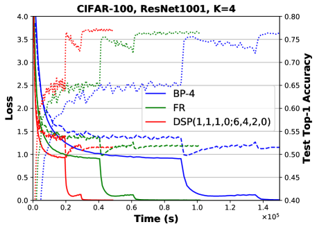
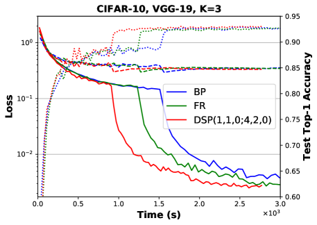
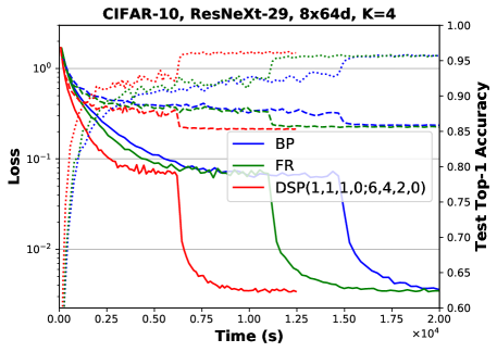
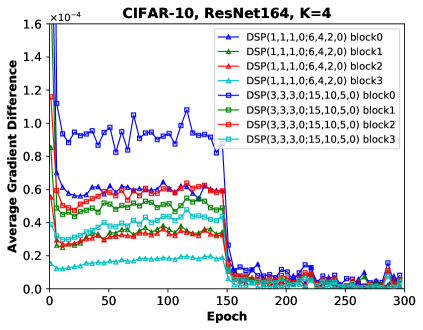
Figure 4: Top left: Average difference of DSP and BP gradient regarding the number of parameters. The rest: Training loss (solid line), testing loss (dash line) and test top-1 accuracy(dot line).

Table 2: Robustness (ResNet164, CIFAR-10, K=3). Each GPU is randomly slowed down.

	Slow down percentage
GPU	20%	50%	100%	150%
FR	8.977%	28.52%	97.06%	359.2%
DSP(1,1,0;4,2,0)	6.017%	16.14%	37.44%	70.99%
DSP(2,2,0;6,3,0)	7.465%	16.01%	36.57%	54.57%
DSP(3,3,0;10,5,0)	7.391%	18.15%	32.10%	53.42%

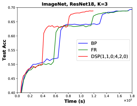
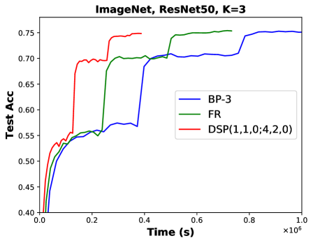
Figure 5: Test accuracy@1 on the ImageNet dataset.

Table 3: Speedup Comparison Results.

	CIFAR-10			CIFAR-100	ImageNet
	ResNet164	ResNext-29	VGG-19	ResNet1001	ResNet50	ResNet101
K, batch size	(4, 128)	(4, 128)	(3, 128)	(4, 128)	(3, 256)	(4, 128)
BP / BP-K	x1 / -	x1 / -	x1 / -	- / x1	- / x1	x1 / -
FR	x1.7	x1.3	x1.1	x1.9	x1.6	x1.7
GPipe	-	-	-	-	-	x2.2
DSP	x2.7	x2.4	x1.5	x4.8	x3.0	x2.7

Experiment Settings

We implement DSP in TensorFlow [1] and run the experiments on Nvidia Tesla P40 GPUs. The model is divided into $K$ blocks and distributed onto $K$ GPUs. Data augmentation procedures include random cropping, random flipping, and standardization. We use SGD with the momentum constant of 0.9. In CIFAR experiments, the batch size is 128. We train ResNet98 and ResNet164 for 300 epochs. The weight decay is $5\times 10^{-4}$ and the initial learning rate is 0.01 (test performance could be a little lower than 0.1 [25]) with a decay of 0.1 at epoch 150, 225; ResNet1001 is trained for 250 epochs. The weight decay is $2\times 10^{-4}$ and the initial learning rate is 0.1 with a decay of 0.1 at epoch 100, 150, 200; VGG-19 and ResNext-29 are trained for 200 epochs. The weight decay is $5\times 10^{-4}$ and the initial learning rate is 0.01 with a decay of 0.1 at epoch 100, 150. We also train ResNet on ImageNet for 90 epochs. The batch size is 256, the weight decay is $1\times 10^{-4}$ and the initial learning rate is 0.1 with a decay of 0.1 at epoch 30, 60, 80. There are four compared methods:

• BP: The standard implementation in TensorFlow. BP (or BP-K) runs on one (or K) GPUs.

• DNI: The Decoupled Neural Interface algorithm in [18]. The auxiliary network consists of two hidden and one output convolution layers with $5\times 5$ filters and padding size of 2. The hidden layers also use batch-normalization and ReLU.

• FR: The Features Replay algorithm proposed by [13].

• DSP: Our Diversely Stale Parameters.

5.1 Faster Training

The DSP convergence curves regarding training epochs are nearly the same as FR and BP, while DNI does not converge as shown in Figure 3. But the epoch time of DSP is much less. Due to the overlap of communication and computation, the overheads of DSP are much less than model parallel BP and the speedup can even exceed $K$. However, it is important that the model should be properly distributed onto different blocks such that the workload of each computing device is balanced. If not, the overall speed will be mostly determined by the slowest device. To further demonstrate the scalability of DSP, we also run experiments on VGG-19 [31], ResNeXt-29 [35], ResNet1001 on the CIFAR dataset, and ResNet18 and ResNet50 on the ImageNet [6] dataset as shown in Figure 4 and Figure 5 respectively. The speedup is summarized in Table 3 (GPipe paper only reports speedup of ResNet101 and AmoebaNet-D (4,512)). Our proposed DSP improves the speedup compared with its counterparts from x0.5 to x3.1 based on different datasets, model and the value of K. Note that the implementation of DSP involves some inefficient copy operations due to limited supported features of the deep learning framework, which means that DSP could achieve a potentially even faster speedup.

5.2 Robustness

To show that DSP is more resilient to the straggle problem due to the FIFO queues introduced, we randomly slow down each GPU by a certain percentage with a probability of $1/3$ and run the experiments on ResNet164 (Table 2). The performance of FR degrades a lot because it does not break the forward locking nor completely decouple the backward pass. In comparison, DSP is very robust with the best slow down percentage always less than $1/3$ of the corresponding GPU slow down percentage. When the upper or lower block suddenly slows down, the current block’s feeding data and gradient queues are less likely to be empty if the length of the queue is long. When the straggler effect is not serious, increasing the Layer-wise Staleness will not bring performance gain; when it is serious instead, DSP benefits a lot from increasing the Layer-wise Staleness. Generally speaking, longer queues improve DSP’s resilience to random stragglers, which is shown in Table 2.

5.3 Generalization

Table 4: Best Top-1 Test Accuracy on ImageNet (K=3).

Method	ResNet18	ResNet50
BP	69.89%	75.35%
FR	68.94%	74.47%
DSP(1,1,0;4,2,0)	68.95%	74.91%

Table 1 and Tabel 4 show the best top-1 test accuracy on the CIFAR and ImageNet dataset respectively. The test performance of DSP is better than BP and FR on the CIFAR dataset. From Lemma 1 we know that the DSP gradient deviates from the BP gradient due to the Layer-wise Staleness. This difference becomes small as the training proceeds but could impose small noise and help find a better local minimum on the comparatively less complex CIFAR classification problem.

In comparison, on the ImageNet dataset, the Layer-wise Staleness can lead to performance degradation. By intuition, it is similar to asynchronous distributed training where the whole gradient is of the same staleness. But in DSP, the more fine-grained Layer-wise Staleness will impose different blocks with different staleness effects. Potential solutions could be using staleness-aware methods as proposed in asynchronous distributed training area, e.g. gradient compensation and staleness-aware learning rate, to alleviate the staleness effect. Another possible direction is to balance the staleness effect between all the blocks. Moreover, when compared with FR, DSP’s test accuracy is slightly better. On ResNet18, the test accuracy of FR and DSP is very similar, but on ResNet50 there is a 0.44% gain using DSP. Besides, on the more complicated ResNet50 architecture, the performance degradation resulting from the staleness effect is smaller than that on ResNet18.

5.4 Gradient Difference

Here we attest our theoretical analysis of Lemma 1 via checking the difference between the DSP and the BP gradient on the CIFAR dataset with the ResNet164 model. From the top-left figure of Figure 4, we can see that the difference between the DSP and BP gradient drops very fast to the converged value as the training proceeds. This difference drops even faster for upper blocks where the Layer-wise Staleness effect is milder. It confirms the motivation behind the DSP algorithm that the DSP gradient will finally be similar to the BP gradient. Moreover, the lower blocks suffer from a larger difference. When the Layer-wise Staleness keeps increasing, the difference will also increase, which matches Lemma 1 well. Moreover, as the learning rate drops, the difference between the DSP gradient and the BP gradient will drop a lot. This implies that a smaller learning rate should be used when we need to deal with a larger number of blocks where the Layer-wise Staleness effect becomes non-trivial. This is also shown in Theorem 1 and 2 that the learning rate should be decreased to make sure it converges at the stated speed.

6 Conclusion

In this paper, we have proposed Layer-wise Staleness and DSP, a novel way to fast train neural networks. DSP is proved to converge to critical points for non-convex problems with SGD and Momentum SGD optimizer. We apply DSP to train CNNs in parallel and the experiment results confirm our theoretical analysis. Our proposed method achieves significant training speedup, strong resilience to random stragglers, better generalization on the CIFAR dataset and reasonable performance on the ImageNet dataset. The speedup can exceed $K$ compared with the model parallel BP. Potential future works include how to alleviate the staleness effect when we need to utilize a further larger number of blocks; how to automatically determine the proper model splitting strategy for load balance among devices; efficiently incorporating DSP with data parallelism to achieve even faster training speed.

Appendix A Queue Size

We mentioned that queue size "$\{q_{k}\}$ is determined by $\{p_{k}\}$ and $\{m_{k}\}$ because the input should match the corresponding error gradient". More specifically, it can be formulated as follows:

$$\begin{cases}&q_{k}=m_{k-1}-p_{k-1}-m_{k}>0\quad\forall k\in\{1,\ldots,K-1\},\\ &q_{0}=0,\\ &m_{k}>0\quad\forall k\in\{0,\ldots,K-1\},\\ &p_{k}>0\quad\forall k\in\{0,\ldots,K-2\},\quad p_{K-1}=0.\\ \end{cases}$$

$q_{0}=0$ and $p_{K-1}=0$ because usually there is no need for the corresponding queue in the first and last block. The first equation ensures that the input and backward error gradient in one block will come from the same data batch.

Appendix B Assumptions

Assumption 1.

(Bounded variance) Assume that the DSP stochastic gradient $\mathcal{G}(x;\xi)$ satisfies:

$$\text{Var}\left[\mathcal{G}(x;\xi)\right]\leq\sigma^{2}.$$

Assumption 2.

(Lipschitz continuous gradient) Assume that the loss and the output of the blocks have Lipschitz continuous gradient, that is, $\forall k\in\{0,1,..,K-1\}$, and $\forall(x_{0,1},...,x_{k,1}),(x_{0,2},...,x_{k,2})\in\mathbb{R}^{d_{0}+d_{1}+...+d_{k}}$,

$$\begin{split}\left\|\nabla F\left(h_{0};x_{0,1};...;x_{k,1}\right)-\nabla F(h_{0};x_{0,2};...;x_{k,2})\right\|\leq L_{k}\left\|(x_{0,1},...,x_{k,1})-(x_{0,2},...,x_{k,2})\right\|,\end{split}$$

and $\forall x_{1}$, $x_{2}\in\mathbb{R}^{d}$,

$$\left\|\nabla f(x_{1})-\nabla f(x_{2})\right\|\leq L_{K}\left\|x_{1}-x_{2}\right\|.$$

Assumption 3.

(Bounded error gradient) Assume that the norm of the error gradient that a block receives is bounded, that is, for any $x\in\mathbb{R}^{d}$, $\forall k\in\{0,1,...,K-2\}$,

$$\begin{split}\left\|\frac{\partial f_{k+1}(h_{k+1};x_{k+1})}{\partial h_{k+1}}...\frac{\partial f_{K-1}(h_{K-1};x_{K-1})}{\partial h_{K-1}}\frac{\partial\mathcal{L}(h_{K},l)}{\partial h_{K}}\right\|\leq M\quad\text{and}\quad\left\|\frac{\partial\mathcal{L}(h_{K},l)}{\partial h_{K}}\right\|\leq M.\end{split}$$

Appendix C Basic Lemmas

Lemma 1.

If Assumptions 2 and 3 hold, the difference between DSP gradient and BP gradient regarding the parameters of block $k$ satisfies:

$$\begin{split}\left\|\nabla_{x_{k}}\mathcal{L}(F(h_{0};x^{t_{0}}_{0};...;x^{t_{K-1}}_{K-1}),y)-\mathcal{G}_{x_{k}}(x^{t_{2K-1}}_{0};...;x^{t_{K}}_{K-1})\right\|\leq LM\sum^{K-1}_{i=k}\left\|x^{t_{2K-1-i}}_{i}-x^{t_{i}}_{i}\right\|.\end{split}$$

Proof.

We gradually move the DSP gradient of the block $k$ towards the BP gradient by replacing one block’s backward parameters with its forward parameters at a time. $K-k$ steps in total are needed, and each step will introduce an error. After all the replacement is done, it becomes the BP gradient at the forward parameters. Firstly we replace $x^{t_{2K-1-k}}_{k}$ with $x^{t_{k}}_{k}$, and calculate the error introduced as follows,

$$\begin{split}\left\|\Delta_{k}\right\|&=\left\|\left(\frac{\partial F(h_{0};x^{t_{0}}_{0};...;x^{t_{k-1}}_{k-1};x^{t_{2K-1-k}}_{k})}{\partial x^{t_{2K-1-k}}_{k}}-\frac{\partial F(h_{0};x^{t_{0}}_{0};...;x^{t_{k-1}}_{k-1};x^{t_{k}}_{k})}{\partial x^{t_{k}}_{k}}\right)\right.\cdot\\ &\quad\frac{\partial F(h_{0};x^{t_{0}}_{0};...;x^{t_{k}}_{k};x^{t_{2K-2-k}}_{k+1})}{\partial F(h_{0};x^{t_{0}}_{0};...;x^{t_{k}}_{k})}\cdots\frac{\partial F(h_{0};x^{t_{0}}_{0};...;x^{t_{K-2}}_{K-2};x^{t_{K}}_{K-1})}{\partial F(h_{0};x^{t_{0}}_{0};...;x^{t_{K-2}}_{K-2})}\cdot\\ &\quad\left.\frac{\partial\mathcal{L}\left(F(h_{0};x^{t_{0}}_{0};...;x^{t_{K-1}}_{K-1}),l\right)}{\partial F(h_{0};x^{t_{0}}_{0};...;x^{t_{K-1}}_{K-1})}\right\|\\ &\leq\left\|\frac{\partial F(h_{0};x^{t_{0}}_{0};...;x^{t_{k-1}}_{k-1};x^{t_{2K-1-k}}_{k})}{\partial x^{t_{2K-1-k}}_{k}}-\frac{\partial F(h_{0};x^{t_{0}}_{0};...;x^{t_{k-1}}_{k-1};x^{t_{k}}_{k})}{\partial x^{t_{k}}_{k}}\right\|\cdot\\ &\quad\left\|\frac{\partial F(h_{0};x^{t_{0}}_{0};...;x^{t_{k}}_{k};x^{t_{2K-2-k}}_{k+1})}{\partial F(h_{0};x^{t_{0}}_{0};...;x^{t_{k}}_{k})}\cdots\frac{\partial F(h_{0};x^{t_{0}}_{0};...;x^{t_{K-2}}_{K-2};x^{t_{K}}_{K-1})}{\partial F(h_{0};x^{t_{0}}_{0};...;x^{t_{K-2}}_{K-2})}\right.\cdot\\ &\quad\left.\frac{\partial\mathcal{L}\left(F(h_{0};x^{t_{0}}_{0};...;x^{t_{K-1}}_{K-1}),l\right)}{\partial F(h_{0};x^{t_{0}}_{0};...;x^{t_{K-1}}_{K-1})}\right\|\\ &\leq LM\left\|x^{t_{2K-1-k}}_{k}-x^{t_{k}}_{k}\right\|.\end{split}$$

Secondly we replace $x^{t_{2K-2-k}}_{k+1}$ with $x^{t_{k+1}}_{k+1}$, and calculate the error introduced,

$$\begin{split}\left\|\Delta_{k+1}\right\|&=\left\|\left(\frac{\partial F(h_{0};x^{t_{0}}_{0};...;x^{t_{k}}_{k};x^{t_{2K-2-k}}_{k+1})}{\partial x^{t_{k}}_{k}}-\frac{\partial F(h_{0};x^{t_{0}}_{0};...;x^{t_{k}}_{k};x^{t_{k+1}}_{k+1})}{\partial x^{t_{k}}_{k}}\right)\right.\cdot\\ &\quad\frac{\partial F(h_{0};x^{t_{0}}_{0};...;x^{t_{k+1}}_{k+1};x^{t_{2K-3-k}}_{k+2})}{\partial F(h_{0};x^{t_{0}}_{0};...;x^{t_{k+1}}_{k+1})}\cdots\frac{\partial F(h_{0};x^{t_{0}}_{0};...;x^{t_{K-2}}_{K-2};x^{t_{K}}_{K-1})}{\partial F(h_{0};x^{t_{0}}_{0};...;x^{t_{K-2}}_{K-2})}\cdot\\ &\quad\left.\frac{\partial\mathcal{L}\left(F(h_{0};x^{t_{0}}_{0};...;x^{t_{K-1}}_{K-1}),l\right)}{\partial F(h_{0};x^{t_{0}}_{0};...;x^{t_{K-1}}_{K-1})}\right\|\\ &\leq\left\|\frac{\partial F(h_{0};x^{t_{0}}_{0};...;x^{t_{k}}_{k};x^{t_{2K-2-k}}_{k+1})}{\partial x^{t_{k}}_{k}}-\frac{\partial F(h_{0};x^{t_{0}}_{0};...;x^{t_{k}}_{k};x^{t_{k+1}}_{k+1})}{\partial x^{t_{k}}_{k}}\right\|\cdot\\ &\quad\left\|\frac{\partial F(h_{0};x^{t_{0}}_{0};...;x^{t_{k+1}}_{k+1};x^{t_{2K-3-k}}_{k+2})}{\partial F(h_{0};x^{t_{0}}_{0};...;x^{t_{k+1}}_{k+1})}\cdots\frac{\partial F(h_{0};x^{t_{0}}_{0};...;x^{t_{K-2}}_{K-2};x^{t_{K}}_{K-1})}{\partial F(h_{0};x^{t_{0}}_{0};...;x^{t_{K-2}}_{K-2})}\right.\cdot\\ &\quad\left.\frac{\partial\mathcal{L}\left(F(h_{0};x^{t_{0}}_{0};...;x^{t_{K-1}}_{K-1}),l\right)}{\partial F(h_{0};x^{t_{0}}_{0};...;x^{t_{K-1}}_{K-1})}\right\|\\ &\leq LM\left\|x^{t_{2K-2-k}}_{k+1}-x^{t_{k+1}}_{k+1}\right\|.\end{split}$$

We repeatedly perform the above procedure, until we get the error in the last step,

$$\begin{split}\left\|\Delta_{K-1}\right\|&=\left\|\left(\frac{\partial F(h_{0};x^{t_{0}}_{0};...;x^{t_{K-2}}_{K-2};x^{t_{K}}_{K-1})}{\partial x^{t_{k}}_{k}}-\frac{\partial F(h_{0};x^{t_{0}}_{0};...;x^{t_{K-2}}_{K-2};x^{t_{K-1}}_{K-1})}{\partial x^{t_{k}}_{k}}\right)\right.\cdot\\ &\quad\left.\frac{\partial\mathcal{L}\left(F(h_{0};x^{t_{0}}_{0};...;x^{t_{K-1}}_{K-1}),l\right)}{\partial F(h_{0};x^{t_{0}}_{0};...;x^{t_{K-1}}_{K-1})}\right\|\\ &\leq\left\|\frac{\partial F(h_{0};x^{t_{0}}_{0};...;x^{t_{K-2}}_{K-2};x^{t_{K}}_{K-1})}{\partial x^{t_{k}}_{k}}-\frac{\partial F(h_{0};x^{t_{0}}_{0};...;x^{t_{K-2}}_{K-2};x^{t_{K-1}}_{K-1})}{\partial x^{t_{k}}_{k}}\right\|\cdot\\ &\quad\left\|\frac{\partial\mathcal{L}\left(F(h_{0};x^{t_{0}}_{0};...;x^{t_{K-1}}_{K-1}),l\right)}{\partial F(h_{0};x^{t_{0}}_{0};...;x^{t_{K-1}}_{K-1})}\right\|\\ &\leq LM\left\|x^{t_{K}}_{K-1}-x^{t_{K-1}}_{K-1}\right\|.\end{split}$$

Add them together and we will have

$$\begin{split}&\left\|\nabla_{x_{k}}\mathcal{L}(F(h_{0};x^{t_{0}}_{0};x^{t_{1}}_{1};...;x^{t_{K-1}}_{K-1}),l)-\mathcal{G}_{x_{k}}(x^{t_{2K-1}}_{0};x^{t_{2K-2}}_{1};...;x^{t_{K}}_{K-1})\right\|\\ &=\left\|\Delta_{k}+\Delta_{k+1}+...+\Delta_{K-1}\right\|\\ &\leq\left\|\Delta_{k}\right\|+\left\|\Delta_{k+1}\right\|+...+\left\|\Delta_{K-1}\right\|\\ &\leq LM\sum^{K-1}_{i=k}\left\|x^{t_{2K-1-i}}_{i}-x^{t_{i}}_{i}\right\|.\end{split}$$

∎

Lemma 2.

Assume Assumption 2 and 3 exist. The second moment of the difference between DSP and BP gradient satisfies,

$$\begin{split}&\left\|\nabla f(x^{t_{0}}_{0};...;x^{t_{K-1}}_{K-1})-\mathcal{G}(x^{t_{2K-1}}_{0};...;x^{t_{K}}_{K-1})\right\|^{2}\leq\frac{1}{2}L^{2}c_{0}\sum^{K-1}_{k=0}\frac{k+1}{K+1}\left\|x^{t_{2K-1-k}}_{k}-x^{t_{k}}_{k}\right\|^{2}.\end{split}$$

Proof.

Via summation of Lemma 1 we can get,

$$\left\|\nabla f(x^{t_{0}}_{0};x^{t_{1}}_{1};...;x^{t_{K-1}}_{K-1})-\mathcal{G}(x^{t_{2K-1}}_{0};x^{t_{2K-2}}_{1};...;x^{t_{K}}_{K-1})\right\|\leq LM\sum^{K-1}_{k=0}(k+1)\left\|x^{t_{2K-1-k}}_{k}-x^{t_{k}}_{k}\right\|.$$

Then we have,

$$\begin{split}&\left\|\nabla f(x^{t_{0}}_{0};x^{t_{1}}_{1};...;x^{t_{K-1}}_{K-1})-\mathcal{G}(x^{t_{2K-1}}_{0};x^{t_{2K-2}}_{1};...;x^{t_{K}}_{K-1})\right\|^{2}\\ &\leq L^{2}M^{2}\left(\sum^{K-1}_{k=0}(k+1)\left\|x^{t_{2K-1-k}}_{k}-x^{t_{k}}_{k}\right\|\right)^{2}\\ &=L^{2}M^{2}\left(\sum^{K-1}_{k=0}(k+1)\right)^{2}\left(\sum^{K-1}_{k=0}\frac{k+1}{\sum^{K-1}_{k=0}(k+1)}\left\|x^{t_{2K-1-k}}_{k}-x^{t_{k}}_{k}\right\|\right)^{2}\\ &\leq L^{2}M^{2}\left(\sum^{K-1}_{k=0}(k+1)\right)^{2}\sum^{K-1}_{k=0}\frac{k+1}{\sum^{K-1}_{k=0}(k+1)}\left\|x^{t_{2K-1-k}}_{k}-x^{t_{k}}_{k}\right\|^{2}\\ &=\frac{1}{2}L^{2}M^{2}K(K+1)\sum^{K-1}_{k=0}(k+1)\left\|x^{t_{2K-1-k}}_{k}-x^{t_{k}}_{k}\right\|^{2}.\\ \end{split}$$

∎

Appendix D DSP with SGD

Theorem 1.

Assume Assumptions 1, 2 and 3 hold. Let $c_{0}=M^{2}K(K+1)^{2}$, and $c_{1}=-(\Delta t^{2}+2)+\sqrt{(\Delta t^{2}+2)^{2}+2c_{0}\Delta t^{2}}$. If the learning rate $\alpha_{n}\leq\frac{c_{1}}{Lc_{0}\Delta t^{2}}$, then

$$\begin{split}\frac{\sum^{N-1}_{n=0}\alpha_{n}\mathbb{E}\left\|\nabla f(x^{n^{\prime}})\right\|^{2}}{\sum^{N-1}_{n=0}\alpha_{n}}\leq\frac{2\left[f(x^{0})-f^{*}\right]}{\sum^{N-1}_{n=0}\alpha_{n}}+\frac{L\sigma^{2}(2+K\Delta t^{2}+\frac{1}{4}Kc_{1})\sum^{N-1}_{n=0}\alpha_{n}^{2}}{\sum^{N-1}_{n=0}\alpha_{n}}.\\ \end{split}$$

Proof.

According to Lipschitz continuous, we have

$$\begin{split}&f(x^{n+1})-f(x^{n})\leq\left\langle\nabla f(x^{n}),x^{n+1}-x^{n}\right\rangle+\frac{L}{2}\left\|x^{n+1}-x^{n}\right\|^{2}\\ &=-\alpha_{n}\left\langle\nabla f(x^{n}),\mathcal{G}(x^{n};\xi)\right\rangle+\frac{L\alpha_{n}^{2}}{2}\left\|\mathcal{G}(x^{n};\xi)\right\|^{2}\\ &=-\alpha_{n}\left\langle\nabla f(x^{n})-\nabla f(x^{n^{\prime}}),\mathcal{G}(x^{n};\xi)\right\rangle-\alpha_{n}\left\langle\nabla f(x^{n^{\prime}}),\mathcal{G}(x^{n};\xi)\right\rangle+\frac{L\alpha^{2}_{n}}{2}\left\|\mathcal{G}(x^{n};\xi)\right\|^{2}\\ &\leq\frac{1}{2L}\left\|\nabla f(x^{n})-\nabla f(x^{n^{\prime}})\right\|^{2}+\frac{L\alpha^{2}_{n}}{2}\left\|\mathcal{G}(x^{n};\xi)\right\|^{2}-\alpha_{n}\left\langle\nabla f(x^{n^{\prime}}),\mathcal{G}(x^{n};\xi)\right\rangle\\ &\quad+\frac{L\alpha^{2}_{n}}{2}\left\|\mathcal{G}(x^{n};\xi)\right\|^{2}\\ &\leq\frac{L}{2}\left\|x^{n}-x^{n^{\prime}}\right\|^{2}-\alpha_{n}\left\langle\nabla f(x^{n^{\prime}}),\mathcal{G}(x^{n};\xi)\right\rangle+L\alpha^{2}_{n}\left\|\mathcal{G}(x^{n};\xi)\right\|^{2}.\\ \end{split}$$

Take expectation regarding $\xi$ on both sides,

$$\begin{split}&\mathbb{E}\left[f(x^{n+1})\right]-f(x^{n})\leq\frac{L}{2}\left\|x^{n}-x^{n^{\prime}}\right\|^{2}-\alpha_{n}\left\langle\nabla f(x^{n^{\prime}}),\mathcal{G}(x^{n})\right\rangle+L\alpha^{2}_{n}\mathbb{E}\left\|\mathcal{G}(x^{n};\xi)\right\|^{2}\\ &=\frac{L}{2}\left\|x^{n}-x^{n^{\prime}}\right\|^{2}+\frac{\alpha_{n}}{2}\left(\left\|\nabla f(x^{n^{\prime}})-\mathcal{G}(x^{n})\right\|^{2}-\left\|\nabla f(x^{n^{\prime}})\right\|^{2}-\left\|\mathcal{G}(x^{n})\right\|^{2}\right)\\ &\quad+L\alpha^{2}_{n}\left(\left\|\mathcal{G}(x^{n})\right\|^{2}+\text{Var}\left[\mathcal{G}(x^{n};\xi)\right]\right)\\ &\leq\frac{L}{2}\left\|x^{n}-x^{n^{\prime}}\right\|^{2}+\frac{\alpha_{n}}{2}\left\|\nabla f(x^{n^{\prime}})-\mathcal{G}(x^{n})\right\|^{2}-\left(\frac{\alpha_{n}}{2}-L\alpha^{2}_{n}\right)\left\|\mathcal{G}(x^{n})\right\|^{2}\\ &\quad-\frac{\alpha_{n}}{2}\left\|\nabla f(x^{n^{\prime}})\right\|^{2}+L\alpha_{n}^{2}\sigma^{2}\\ &\leq\sum^{K-1}_{k=0}\left[\frac{L}{2}+\frac{1}{4}\alpha_{n}L^{2}M^{2}K(K+1)(k+1)\right]\left\|x^{n}_{k}-x^{n^{\prime}}_{k}\right\|^{2}-\left(\frac{\alpha_{n}}{2}-L\alpha^{2}_{n}\right)\left\|\mathcal{G}(x^{n})\right\|^{2}\\ &\quad-\frac{\alpha_{n}}{2}\left\|\nabla f(x^{n^{\prime}})\right\|^{2}+L\alpha_{n}^{2}\sigma^{2}.\\ \end{split}$$

The last inequality utilizes Lemma 2. Consider the first term and take expectation,

$$\begin{split}\mathbb{E}\left\|x^{n}_{k}-x^{n^{\prime}}_{k}\right\|^{2}&=\mathbb{E}\left\|\sum^{n-1}_{i=n-\Delta t_{k}}-\alpha_{i}\mathcal{G}_{x_{k}}(x^{i};\xi)\right\|^{2}\\ &\leq\Delta t_{k}\sum^{n-1}_{i=n-\Delta t_{k}}\alpha_{i}^{2}\mathbb{E}\left\|\mathcal{G}_{x^{k}}(x^{i};\xi)\right\|^{2}\\ &\leq\Delta t\sum^{n-1}_{i=n-\Delta t}\alpha_{i}^{2}\left(\left\|\mathcal{G}_{x_{k}}(x^{i})\right\|^{2}+\sigma^{2}\right).\\ \end{split}$$

Take the total expectation and perform summation for it,

$$\begin{split}&\sum^{N-1}_{n=0}\sum^{K-1}_{k=0}\left(\frac{L}{2}+\frac{1}{4}\alpha_{n}L^{2}M^{2}K(K+1)(k+1)\right)\mathbb{E}\left\|x^{n}_{k}-x^{n^{\prime}}_{k}\right\|^{2}\\ &\leq\sum^{N-1}_{n=0}\sum^{K-1}_{k=0}\left(\frac{L}{2}+\frac{1}{4}\alpha_{n}L^{2}M^{2}K(K+1)(k+1)\right)\Delta t\sum^{n-1}_{i=n-\Delta t}\alpha_{i}^{2}\left(\mathbb{E}\left\|\mathcal{G}_{x_{k}}(x^{i})\right\|^{2}+\sigma^{2}\right)\\ &\leq\sum^{N-1}_{n=0}\sum^{K-1}_{k=0}\left(\frac{L}{2}+\frac{1}{4}\alpha_{n}L^{2}M^{2}K(K+1)(k+1)\right)\Delta t\cdot\Delta t\cdot\alpha_{n}^{2}\left(\mathbb{E}\left\|\mathcal{G}_{x_{k}}(x^{n})\right\|^{2}+\sigma^{2}\right).\end{split}$$

Take the total expectation and perform summation for all the terms,

$$\begin{split}&\mathbb{E}\left[f(x^{N})\right]-f(x^{0})\\ &\leq\sum^{N-1}_{n=0}\sum^{K-1}_{k=0}\left(\frac{L}{2}+\frac{1}{4}\alpha_{n}L^{2}M^{2}K(K+1)(k+1)\right)\Delta t^{2}\alpha_{n}^{2}\left(\mathbb{E}\left\|\mathcal{G}_{x_{k}}(x^{n})\right\|^{2}+\sigma^{2}\right)\\ &\quad-\sum^{N-1}_{n=0}\left(\frac{\alpha_{n}}{2}-L\alpha_{n}^{2}\right)\mathbb{E}\sum^{K-1}_{k=0}\left\|\mathcal{G}_{x_{k}}(x^{n})\right\|^{2}-\sum^{N-1}_{n=0}\frac{\alpha_{n}}{2}\mathbb{E}\left\|\nabla f(x^{n^{\prime}})\right\|^{2}+L\sigma^{2}\sum^{N-1}_{n=0}\alpha_{n}^{2}\\ &=\sum^{N-1}_{n=0}\sum^{K-1}_{k=0}\left(\left(\frac{L}{2}+\frac{1}{4}\alpha_{n}L^{2}M^{2}K(K+1)(k+1)\right)\Delta t^{2}\alpha_{n}^{2}-\frac{\alpha_{n}}{2}+L\alpha_{n}^{2}\right)\mathbb{E}\left\|\mathcal{G}_{x_{k}}(x^{n})\right\|^{2}\\ &\quad+\sum^{N-1}_{n=0}\sum^{K-1}_{k=0}\left(\frac{L}{2}+\frac{1}{4}\alpha_{n}L^{2}M^{2}K(K+1)(k+1)\right)\Delta t^{2}\alpha_{n}^{2}\sigma^{2}-\sum^{N-1}_{n=0}\frac{\alpha_{n}}{2}\mathbb{E}\left\|\nabla f(x^{n^{\prime}})\right\|^{2}\\ &\quad+L\sigma^{2}\sum^{N-1}_{n=0}\alpha_{n}^{2}\\ &\leq\sum^{N-1}_{n=0}\sum^{K-1}_{k=0}\frac{1}{4}\alpha_{n}\left(L^{2}M^{2}K(K+1)^{2}\Delta t^{2}\alpha_{n}^{2}+\left(2\Delta t^{2}+4\right)L\alpha_{n}-2\right)\mathbb{E}\left\|\mathcal{G}_{x^{k}}(x^{n})\right\|^{2}\\ &\quad+\sum^{N-1}_{n=0}\left(\frac{1}{2}LK+\frac{1}{8}\alpha_{n}L^{2}M^{2}K^{2}(K+1)^{2}\right)\Delta t^{2}\alpha_{n}^{2}\sigma^{2}-\sum^{N-1}_{n=0}\frac{\alpha_{n}}{2}\mathbb{E}\left\|\nabla f(x^{n^{\prime}})\right\|^{2}+L\sigma^{2}\sum^{N-1}_{n=0}\alpha_{n}^{2}\\ &\leq\sum^{N-1}_{n=0}\left(\frac{1}{2}LK+\frac{1}{8}\alpha_{n}L^{2}M^{2}K^{2}(K+1)^{2}\right)\Delta t^{2}\alpha_{n}^{2}\sigma^{2}-\sum^{N-1}_{n=0}\frac{\alpha_{n}}{2}\mathbb{E}\left\|\nabla f(x^{n^{\prime}})\right\|^{2}+L\sigma^{2}\sum^{N-1}_{n=0}\alpha_{n}^{2}.\\ \end{split}$$

The last inequality utilizes the restriction on the learning rate. Then we have

$$\begin{split}&\frac{\sum^{N-1}_{n=0}\alpha_{n}\mathbb{E}\left\|\nabla f(x^{n^{\prime}})\right\|^{2}}{\sum^{N-1}_{n=0}\alpha_{n}}\\ &\leq\frac{2\left[f(x^{0})-f^{*}\right]}{\sum^{N-1}_{n=0}\alpha_{n}}+\frac{L\sigma^{2}\sum^{N-1}_{n=0}\alpha_{n}^{2}\left[2+K\Delta t^{2}+\frac{1}{4}\alpha_{n}LM^{2}K^{2}(K+1)^{2}\Delta t^{2}\right]}{\sum^{N-1}_{n=0}\alpha_{n}}.\end{split}$$

∎

Appendix E DSP with Momentum SGD

The SUM method also implies the following recursions,

$$\begin{split}x^{n+1}+\frac{\beta}{1-\beta}v^{n+1}&=x^{n}+\frac{\beta}{1-\beta}v^{n}-\frac{\alpha}{1-\beta}\mathcal{G}(x^{n};\xi),\quad n\geq 0\\ v^{n+1}&=\beta v^{n}+((1-\beta)s-1)\alpha\mathcal{G}(x^{n};\xi),\quad n\geq 0.\end{split}$$ (6)

where $v^{n}$ is given by

$$v^{n}=\begin{cases}x^{n}-x^{n-1}+s\alpha\mathcal{G}(x^{n-1};\xi),\quad n\geq 1\\ 0,\quad n=0.\end{cases}$$ (7)

Let $z^{n}=x^{n}+\frac{\beta}{1-\beta}v^{n}$.

Lemma 3.

Assume Assumption 1 exists. Let $c_{2}=\frac{\left((1-\beta)s-1\right)^{2}}{(1-\beta)^{2}}$, then

$$\sum^{N-1}_{n=0}\mathbb{E}\left\|v^{n}\right\|^{2}\leq c_{2}\alpha^{2}\sum^{N-1}_{n=0}\mathbb{E}\left\|\mathcal{G}(x^{n})\right\|^{2}+c_{2}\sigma^{2}\alpha^{2}N.$$

Proof.

Let $\hat{\alpha}=((1-\beta)s-1)\alpha$. From Eq. (6),

$$v^{n+1}=\beta v^{n}+\hat{\alpha}\mathcal{G}(x^{n};\xi).$$

Note that $v^{0}=0$. Then

$$v^{n}=\hat{\alpha}\sum^{n-1}_{i=0}\beta^{n-1-i}\mathcal{G}(x^{i};\xi).$$

Then we have,

$$\begin{split}\mathbb{E}\left\|v^{n}\right\|^{2}&=\hat{\alpha}^{2}\mathbb{E}\left\|\sum^{n-1}_{i=0}\beta^{n-1-i}\mathcal{G}(x^{i};\xi)\right\|^{2}=\hat{\alpha}^{2}\left(\sum^{n-1}_{i=0}\beta^{n-1-i}\right)^{2}\mathbb{E}\left\|\sum^{n-1}_{i=0}\frac{\beta^{n-1-i}}{\sum^{n-1}_{i=0}\beta^{n-1-i}}\mathcal{G}(x^{i};\xi)\right\|^{2}\\ &\leq\hat{\alpha}^{2}\left(\sum^{n-1}_{i=0}\beta^{n-1-i}\right)^{2}\sum^{n-1}_{i=0}\frac{\beta^{n-1-i}}{\sum^{n-1}_{i=0}\beta^{n-1-i}}\mathbb{E}\left\|\mathcal{G}(x^{i};\xi)\right\|^{2}\\ &=\hat{\alpha}^{2}\sum^{n-1}_{i=0}\beta^{n-1-i}\sum^{n-1}_{i=0}\beta^{n-1-i}\left\|\mathcal{G}(x^{i})\right\|^{2}+\hat{\alpha}^{2}\sigma^{2}\left(\sum^{n-1}_{i=0}\beta^{n-1-i}\right)^{2}\\ &\leq\frac{\hat{\alpha}^{2}}{1-\beta}\sum^{n-1}_{i=0}\beta^{n-1-i}\left\|\mathcal{G}(x^{i})\right\|^{2}+\frac{\hat{\alpha}^{2}\sigma^{2}}{(1-\beta)^{2}}\\ &=(1-\beta)c_{2}\alpha^{2}\sum^{n-1}_{i=0}\beta^{n-1-i}\left\|\mathcal{G}(x^{i})\right\|^{2}+c_{2}\alpha^{2}\sigma^{2}.\\ \end{split}$$

Take the total expectation and perform summation,

$$\begin{split}\sum^{N-1}_{n=0}\mathbb{E}\left[\left\|v^{n}\right\|^{2}\right]&\leq(1-\beta)c_{2}\alpha^{2}\sum^{N-1}_{n=0}\sum^{n-1}_{i=0}\beta^{n-1-i}\mathbb{E}\left\|\mathcal{G}(x^{i})\right\|^{2}+c_{2}\alpha^{2}\sigma^{2}N\\ &=(1-\beta)c_{2}\alpha^{2}\sum^{N-2}_{i=0}\sum^{N-1}_{n=i+1}\beta^{n-1-i}\mathbb{E}\left\|\mathcal{G}(x^{i})\right\|^{2}+c_{2}\alpha^{2}\sigma^{2}N\\ &=(1-\beta)c_{2}\alpha^{2}\sum^{N-2}_{i=0}\frac{1-\beta^{N-1-i}}{1-\beta}\mathbb{E}\left\|\mathcal{G}(x^{i})\right\|^{2}+c_{2}\alpha^{2}\sigma^{2}N\\ &\leq c_{2}\alpha^{2}\sum^{N-2}_{n=0}\mathbb{E}\left\|\mathcal{G}(x^{n})\right\|^{2}+c_{2}\sigma^{2}\alpha^{2}N\leq c_{2}\alpha^{2}\sum^{N-1}_{n=0}\mathbb{E}\left\|\mathcal{G}(x^{n})\right\|^{2}+c_{2}\sigma^{2}\alpha^{2}N.\\ \end{split}$$

∎

Lemma 4.

Assume Assumption 1 exists, then

$$\begin{split}\sum^{N-1}_{n=0}\mathbb{E}\left\|x^{n}-x^{n^{\prime}}\right\|^{2}&\leq 2\Delta t^{2}(c_{2}+s^{2})\alpha^{2}\sum^{N-1}_{n=0}\mathbb{E}\left\|\mathcal{G}(x^{n})\right\|^{2}+2\Delta t^{2}\sigma^{2}(c_{2}+s^{2})\alpha^{2}N.\\ \end{split}$$

Proof.

First take expectation regarding $\xi$,

$$\begin{split}\mathbb{E}\left\|x^{n}-x^{n^{\prime}}\right\|^{2}&=\sum^{K-1}_{k=0}\mathbb{E}\left\|x^{n}_{k}-x^{n^{\prime}}_{k}\right\|^{2}=\sum^{K-1}_{k=0}\mathbb{E}\left\|\sum^{n-1}_{i=n-\Delta t_{k}}v^{i+1}_{k}-s\alpha\mathcal{G}_{x_{k}}(x^{i};\xi)\right\|^{2}\\ &\leq\sum^{K-1}_{k=0}\Delta t_{k}\sum^{n-1}_{i=n-\Delta t_{k}}\mathbb{E}\left\|v^{i+1}_{k}-s\alpha\mathcal{G}_{x_{k}}(x^{i};\xi)\right\|^{2}\\ &\leq\sum^{K-1}_{k=0}2\Delta t_{k}\sum^{n-1}_{i=n-\Delta t_{k}}\left(\mathbb{E}\left\|v^{i+1}_{k}\right\|^{2}+s^{2}\alpha^{2}\mathbb{E}\left\|\mathcal{G}_{x_{k}}(x^{i};\xi)\right\|^{2}\right)\\ &\leq\sum^{K-1}_{k=0}2\Delta t\sum^{n-1}_{i=n-\Delta t}\left(\mathbb{E}\left\|v^{i+1}_{k}\right\|^{2}+s^{2}\alpha^{2}\mathbb{E}\left\|\mathcal{G}_{x_{k}}(x^{i};\xi)\right\|^{2}\right)\\ &=2\Delta t\sum^{n-1}_{i=n-\Delta t}\left(\mathbb{E}\left\|v^{i+1}\right\|^{2}+s^{2}\alpha^{2}\mathbb{E}\left\|\mathcal{G}(x^{i};\xi)\right\|^{2}\right)\\ &\leq 2\Delta t\sum^{n-1}_{i=n-\Delta t}\left(\mathbb{E}\left\|v^{i+1}\right\|^{2}+s^{2}\alpha^{2}\left\|\mathcal{G}(x^{i})\right\|^{2}+s^{2}\alpha^{2}\sigma^{2}\right).\\ \end{split}$$

Take total expectation on both sides and perform summation,

$$\begin{split}\sum^{N-1}_{n=0}\mathbb{E}\left\|x^{n}-x^{n^{\prime}}\right\|^{2}&\leq 2\Delta t\sum^{N-1}_{n=0}\sum^{n-1}_{i=n-\Delta t}\left(\mathbb{E}\left\|v^{i+1}\right\|^{2}+s^{2}\alpha^{2}\mathbb{E}\left\|\mathcal{G}(x^{i})\right\|^{2}+s^{2}\alpha^{2}\sigma^{2}\right)\\ &\leq 2\Delta t^{2}\sum^{N-2}_{n=0}\left(\mathbb{E}\left\|v^{n+1}\right\|^{2}+s^{2}\alpha^{2}\mathbb{E}\left\|\mathcal{G}(x^{n})\right\|^{2}+s^{2}\alpha^{2}\sigma^{2}\right)\\ &\leq 2\Delta t^{2}\sum^{N-1}_{n=0}\mathbb{E}\left\|v^{n}\right\|^{2}+2\Delta t^{2}s^{2}\alpha^{2}\sum^{N-1}_{n=0}\mathbb{E}\left\|\mathcal{G}(x^{n})\right\|^{2}+2\Delta t^{2}s^{2}\alpha^{2}\sigma^{2}N\\ &\leq 2\Delta t^{2}(c_{2}+s^{2})\alpha^{2}\sum^{N-1}_{n=0}\mathbb{E}\left[\left\|\mathcal{G}(x^{n})\right\|^{2}\right]+2\Delta t^{2}\sigma^{2}(c_{2}+s^{2})\alpha^{2}N.\\ \end{split}$$

∎

Theorem 2.

Assume Assumption 1, 2 and 3 hold. Let $c_{2}=\frac{((1-\beta)s-1)^{2}}{(1-\beta)^{2}}$, $c_{3}=M^{2}K(K+1)^{2}\Delta t^{2}(c_{2}+s^{2})$, $c_{4}=3+\beta^{2}c_{2}+2(1-\beta)^{2}\Delta t^{2}(c_{2}+s^{2})$, and $c_{5}=\frac{2+\beta^{2}c_{2}}{1-\beta}+2(1-\beta)\Delta t^{2}(c_{2}+s^{2})+\frac{-c_{4}+\sqrt{c_{4}^{2}+4(1-\beta)^{2}c_{3}}}{2(1-\beta)}$. If the learning rate $\alpha$ is fixed and satisfies $\quad\alpha\leq\frac{-c_{4}+\sqrt{c_{4}^{2}+4(1-\beta)^{2}c_{3}}}{2(1-\beta)c_{3}L}$, then

$$\frac{1}{N}\sum^{N-1}_{n=0}\mathbb{E}\left\|\nabla f(x^{n^{\prime}})\right\|^{2}\leq\frac{2(1-\beta)(f(x^{0})-f^{*})}{N\alpha}+c_{5}\sigma^{2}L\alpha.$$

Proof.

According to Lipschitz continuous gradient,

$$\begin{split}&f(z^{n+1})-f(z^{n})\\ &\leq\left\langle\nabla f(z^{n}),z^{n+1}-z^{n}\right\rangle+\frac{L}{2}\left\|z^{n+1}-z^{n}\right\|^{2}\\ &=-\frac{\alpha}{1-\beta}\left\langle\nabla f(z^{n}),\mathcal{G}(x^{n};\xi)\right\rangle+\frac{L\alpha^{2}}{2(1-\beta)^{2}}\left\|\mathcal{G}(x^{n};\xi)\right\|^{2}\\ &=-\frac{\alpha}{1-\beta}\left\langle\nabla f(z^{n})-\nabla f(x^{n}),\mathcal{G}(x^{n};\xi)\right\rangle-\frac{\alpha}{1-\beta}\left\langle\nabla f(x^{n}),\mathcal{G}(x^{n};\xi)\right\rangle\\ &\quad+\frac{L\alpha^{2}}{2(1-\beta)^{2}}\left\|\mathcal{G}(x^{n};\xi)\right\|^{2}\\ &\leq\frac{1}{2}\left(\frac{1}{L}\left\|\nabla f(z^{n})-\nabla f(x^{n})\right\|^{2}+\frac{L\alpha^{2}}{(1-\beta)^{2}}\left\|\mathcal{G}(x^{n};\xi)\right\|^{2}\right)\\ &\quad-\frac{\alpha}{1-\beta}\left\langle\nabla f(x^{n}),\mathcal{G}(x^{n};\xi)\right\rangle+\frac{L\alpha^{2}}{2(1-\beta)^{2}}\left\|\mathcal{G}(x^{n};\xi)\right\|^{2}\\ &=\frac{1}{2L}\left\|\nabla f(z^{n})-\nabla f(x^{n})\right\|^{2}-\frac{\alpha}{1-\beta}\left\langle\nabla f(x^{n}),\mathcal{G}(x^{n};\xi)\right\rangle+\frac{L\alpha^{2}}{(1-\beta)^{2}}\left\|\mathcal{G}(x^{n};\xi)\right\|^{2}.\\ \end{split}$$

Take expectation regarding $\xi$ on both sides,

$$\begin{split}&\mathbb{E}\left[f(z^{n+1})\right]-f(z^{n})\\ &\leq\frac{1}{2L}\left\|\nabla f(z^{n})-\nabla f(x^{n})\right\|^{2}-\frac{\alpha}{1-\beta}\left\langle\nabla f(x^{n}),\mathcal{G}(x^{n})\right\rangle+\frac{L\alpha^{2}}{(1-\beta)^{2}}\left\|\mathcal{G}(x^{n})\right\|^{2}+\frac{L\alpha^{2}}{(1-\beta)^{2}}\sigma^{2}\\ &=\frac{1}{2L}\left\|\nabla f(z^{n})-\nabla f(x^{n})\right\|^{2}-\frac{\alpha}{1-\beta}\left\langle\nabla f(x^{n})-\nabla f(x^{n^{\prime}}),\mathcal{G}(x^{n})\right\rangle\\ &\quad-\frac{\alpha}{1-\beta}\left\langle\nabla f(x^{n^{\prime}}),\mathcal{G}(x^{n})\right\rangle+\frac{L\alpha^{2}}{(1-\beta)^{2}}\left\|\mathcal{G}(x^{n})\right\|^{2}+\frac{L\alpha^{2}}{(1-\beta)^{2}}\sigma^{2}\\ &\leq\frac{1}{2L}\left\|\nabla f(z^{n})-\nabla f(x^{n})\right\|^{2}+\frac{1}{2}\left(\frac{1}{L}\left\|\nabla f(x^{n})-\nabla f(x^{n^{\prime}})\right\|^{2}+\frac{L\alpha^{2}}{(1-\beta)^{2}}\left\|\mathcal{G}(x^{n})\right\|^{2}\right)\\ &\quad+\frac{\alpha}{2(1-\beta)}\left(\left\|\nabla f(x^{n^{\prime}})-\mathcal{G}(x^{n})\right\|^{2}-\left\|\nabla f(x^{n^{\prime}})\right\|^{2}-\left\|\mathcal{G}(x^{n})\right\|^{2}\right)\\ &\quad+\frac{L\alpha^{2}}{(1-\beta)^{2}}\left\|\mathcal{G}(x^{n})\right\|^{2}+\frac{L\alpha^{2}}{(1-\beta)^{2}}\sigma^{2}\\ &=-\frac{\alpha}{2(1-\beta)}\left\|\nabla f(x^{n^{\prime}})\right\|^{2}+\frac{1}{2L}\left\|\nabla f(z^{n})-\nabla f(x^{n})\right\|^{2}+\frac{1}{2L}\left\|\nabla f(x^{n})-\nabla f(x^{n^{\prime}})\right\|^{2}\\ &\quad+\frac{\alpha}{2(1-\beta)}\left\|\nabla f(x^{n^{\prime}})-\mathcal{G}(x^{n})\right\|^{2}-\left(\frac{\alpha}{2(1-\beta)}-\frac{3L\alpha^{2}}{2(1-\beta)^{2}}\right)\left\|\mathcal{G}(x^{n})\right\|^{2}+\frac{L\alpha^{2}}{(1-\beta)^{2}}\sigma^{2}.\\ \end{split}$$

Take the total expectation and perform summation,

$$\begin{split}\sum^{N-1}_{n=0}\mathbb{E}\left[\frac{1}{2L}\left\|\nabla f(z^{n})-\nabla f(x^{n})\right\|^{2}\right]&\leq\sum^{N-1}_{n=0}\frac{L}{2}\mathbb{E}\left\|z^{n}-x^{n}\right\|^{2}=\sum^{N-1}_{n=0}\frac{L\beta^{2}}{2(1-\beta)^{2}}\mathbb{E}\left\|v^{n}\right\|^{2}.\end{split}$$

$$\begin{split}&\sum^{N-1}_{n=0}\mathbb{E}\left[\frac{1}{2L}\left\|\nabla f(x^{n})-\nabla f(x^{n^{\prime}})\right\|^{2}+\frac{\alpha}{2(1-\beta)}\left\|\nabla f(x^{n^{\prime}})-\mathcal{G}(x^{n})\right\|^{2}\right]\\ &\leq\sum^{N-1}_{n=0}\frac{L}{2}\mathbb{E}\left\|x^{n}-x^{n^{\prime}}\right\|^{2}+\frac{\alpha}{4(1-\beta)}L^{2}M^{2}K(K+1)\sum^{K-1}_{k=0}(k+1)\sum^{N-1}_{n=0}\mathbb{E}\left\|x^{n}_{k}-x^{n^{\prime}}_{k}\right\|^{2}\\ &\leq\sum^{N-1}_{n=0}\frac{L}{2}\mathbb{E}\left\|x^{n}-x^{n^{\prime}}\right\|^{2}+\frac{\alpha}{4(1-\beta)}L^{2}M^{2}K(K+1)^{2}\sum^{N-1}_{n=0}\mathbb{E}\left\|x^{n}-x^{n^{\prime}}\right\|^{2}\\ &\leq\sum^{N-1}_{n=0}\frac{L}{2}\left(1+\frac{\alpha}{2(1-\beta)}LM^{2}K(K+1)^{2}\right)\mathbb{E}\left\|x^{n}-x^{n^{\prime}}\right\|^{2}.\end{split}$$

Then we have,

$$\begin{split}&\mathbb{E}\left[f(z^{N})\right]-f(z^{0})\\ &\leq-\frac{\alpha}{2(1-\beta)}\sum^{N-1}_{n=0}\mathbb{E}\left\|\nabla f(x^{n^{\prime}})\right\|^{2}-\left(\frac{\alpha}{2(1-\beta)}-\frac{3L\alpha^{2}}{2(1-\beta)^{2}}\right)\sum^{N-1}_{n=0}\mathbb{E}\left\|\mathcal{G}(x^{n})\right\|^{2}+\frac{L\sigma^{2}\alpha^{2}}{(1-\beta)^{2}}N\\ &\quad+\sum^{N-1}_{n=0}\frac{L\beta^{2}}{2(1-\beta)^{2}}\mathbb{E}\left\|v^{n}\right\|^{2}+\sum^{N-1}_{n=0}\frac{L}{2}\left(1+\frac{\alpha}{2(1-\beta)}LM^{2}K(K+1)^{2}\right)\mathbb{E}\left\|x^{n}-x^{n^{\prime}}\right\|^{2}\\ &\leq-\frac{\alpha}{2(1-\beta)}\sum^{N-1}_{n=0}\mathbb{E}\left\|\nabla f(x^{n^{\prime}})\right\|^{2}-\left(\frac{\alpha}{2(1-\beta)}-\frac{3L\alpha^{2}}{2(1-\beta)^{2}}\right)\sum^{N-1}_{n=0}\mathbb{E}\left\|\mathcal{G}(x^{n})\right\|^{2}+\frac{L\sigma^{2}\alpha^{2}}{(1-\beta)^{2}}N\\ &\quad+\frac{L\beta^{2}}{2(1-\beta)^{2}}\left(c_{2}\alpha^{2}\sum^{N-1}_{n=0}\mathbb{E}\left\|\mathcal{G}(x^{n})\right\|^{2}+c_{2}\sigma^{2}\alpha^{2}N\right)\\ &\quad+\frac{L}{2}\left(1+\frac{\alpha}{2(1-\beta)}LM^{2}K(K+1)^{2}\right)\cdot\\ &\quad\quad\left[2\Delta t^{2}(c_{2}+s^{2})\alpha^{2}\sum^{N-1}_{n=0}\mathbb{E}\left\|\mathcal{G}(x^{n})\right\|^{2}+2\Delta t^{2}\sigma^{2}(c_{2}+s^{2})\alpha^{2}N\right]\\ &=-\frac{\alpha}{2(1-\beta)}\sum^{N-1}_{n=0}\mathbb{E}\left\|\nabla f(x^{n^{\prime}})\right\|^{2}-\left[\frac{\alpha}{2(1-\beta)}-\alpha^{2}\left(\frac{3L}{2(1-\beta)^{2}}+\frac{L\beta^{2}c_{2}}{2(1-\beta)^{2}}\right.\right.+\\ &\quad\quad\left.\left.L\left(1+\frac{\alpha}{2(1-\beta)}LM^{2}K(K+1)^{2}\right)\Delta t^{2}(c_{2}+s^{2})\right)\right]\cdot\sum^{N-1}_{n=0}\mathbb{E}\left\|\mathcal{G}(x^{n})\right\|^{2}\\ &\quad+\sigma^{2}\alpha^{2}N\left[\frac{L}{(1-\beta)^{2}}+\frac{L\beta^{2}c_{2}}{2(1-\beta)^{2}}+L\left(1+\frac{\alpha}{2(1-\beta)}LM^{2}K(K+1)^{2}\right)\Delta t^{2}(c_{2}+s^{2})\right]\\ &=-\frac{\alpha}{2(1-\beta)}\sum^{N-1}_{n=0}\mathbb{E}\left\|\nabla f(x^{n^{\prime}})\right\|^{2}+\frac{\alpha}{2(1-\beta)^{2}}[(1-\beta)M^{2}K(K+1)^{2}\Delta t^{2}(c_{2}+s^{2})L^{2}\alpha^{2}+\\ &\quad\quad\left(3+\beta^{2}c_{2}+2(1-\beta)^{2}\Delta t^{2}(c_{2}+s^{2})\right)L\alpha-(1-\beta)]\cdot\sum^{N-1}_{n=0}\mathbb{E}\left\|\mathcal{G}(x^{n})\right\|^{2}\\ &\quad+\sigma^{2}\alpha^{2}N\left[\frac{L}{(1-\beta)^{2}}+\frac{L\beta^{2}c_{2}}{2(1-\beta)^{2}}+L\left(1+\frac{\alpha}{2(1-\beta)}LM^{2}K(K+1)^{2}\right)\Delta t^{2}(c_{2}+s^{2})\right].\\ \end{split}$$

The second inequality utilizes Lemma 3 and 4. According to the restriction on the learning rate, we can remove the second term in the last equality,

$$\begin{split}f_{*}-f(x^{0})&\leq-\frac{\alpha}{2(1-\beta)}\sum^{N-1}_{n=0}\mathbb{E}\left\|\nabla f(x^{n^{\prime}})\right\|^{2}+\sigma^{2}L\alpha^{2}N\left[\frac{1}{(1-\beta)^{2}}+\frac{\beta^{2}c_{2}}{2(1-\beta)^{2}}\right.+\\ &\quad\quad\left.\left(1+\frac{\alpha}{2(1-\beta)}LM^{2}K(K+1)^{2}\right)\Delta t^{2}(c_{2}+s^{2})\right].\\ \end{split}$$

Therefore we have,

$$\begin{split}\frac{1}{N}\sum^{N-1}_{n=0}\mathbb{E}\left\|\nabla f(x^{n^{\prime}})\right\|^{2}&\leq\frac{2(1-\beta)(f^{*}-f(x^{0}))}{N\alpha}\\ &\quad+\sigma^{2}L\alpha\left[\frac{2+\beta^{2}c_{2}}{1-\beta}+\left(2(1-\beta)+\alpha LM^{2}K(K+1)^{2}\right)\Delta t^{2}(c_{2}+s^{2})\right].\\ \end{split}$$

∎

References

• [1] Martín Abadi, Paul Barham, Jianmin Chen, Zhifeng Chen, Andy Davis, Jeffrey Dean, Matthieu Devin, Sanjay Ghemawat, Geoffrey Irving, Michael Isard, et al. Tensorflow: A system for large-scale machine learning. In 12th USENIX Symposium on Operating Systems Design and Implementation (OSDI’ 16), pages 265--283, 2016.
• [2] Eugene Belilovsky, Michael Eickenberg, and Edouard Oyallon. Decoupled greedy learning of cnns. arXiv preprint arXiv:1901.08164, 2019.
• [3] Léon Bottou. Large-scale machine learning with stochastic gradient descent. In Yves Lechevallier and Gilbert Saporta, editors, Proceedings of COMPSTAT’2010, pages 177--186, Heidelberg, 2010. Physica-Verlag HD.
• [4] Tianqi Chen, Mu Li, Yutian Li, Min Lin, Naiyan Wang, Minjie Wang, Tianjun Xiao, Bing Xu, Chiyuan Zhang, and Zheng Zhang. Mxnet: A flexible and efficient machine learning library for heterogeneous distributed systems. arXiv preprint arXiv:1512.01274, 2015.
• [5] Tianqi Chen, Bing Xu, Chiyuan Zhang, and Carlos Guestrin. Training deep nets with sublinear memory cost. arXiv preprint arXiv:1604.06174, 2016.
• [6] Jia Deng, Wei Dong, Richard Socher, Li-Jia Li, Kai Li, and Li Fei-Fei. Imagenet: A large-scale hierarchical image database. In 2009 IEEE conference on computer vision and pattern recognition, pages 248--255. Ieee, 2009.
• [7] Andreas Griewank. An implementation of checkpointing for the reverse or adjoint model of differentiation. ACM Trans. Math. Software, 26(1):1--19, 1999.
• [8] Kaiming He, Xiangyu Zhang, Shaoqing Ren, and Jian Sun. Delving deep into rectifiers: Surpassing human-level performance on imagenet classification. In Proceedings of the IEEE international conference on computer vision, pages 1026--1034, 2015.
• [9] Qirong Ho, James Cipar, Henggang Cui, Seunghak Lee, Jin Kyu Kim, Phillip B Gibbons, Garth A Gibson, Greg Ganger, and Eric P Xing. More effective distributed ml via a stale synchronous parallel parameter server. In Advances in neural information processing systems, pages 1223--1231, 2013.
• [10] Jie Hu, Li Shen, and Gang Sun. Squeeze-and-excitation networks. In Proceedings of the IEEE conference on computer vision and pattern recognition, pages 7132--7141, 2018.
• [11] Yanping Huang, Yonglong Cheng, Dehao Chen, HyoukJoong Lee, Jiquan Ngiam, Quoc V Le, and Zhifeng Chen. Gpipe: Efficient training of giant neural networks using pipeline parallelism. arXiv preprint arXiv:1811.06965, 2018.
• [12] Yuzhen Huang, Xiao Yan, Guanxian Jiang, Tatiana Jin, James Cheng, An Xu, Zhanhao Liu, and Shuo Tu. Tangram: bridging immutable and mutable abstractions for distributed data analytics. In 2019 {{\{USENIX}}\} Annual Technical Conference ({{\{USENIX}}\}{{\{ATC}}\} 19), pages 191--206, 2019.
• [13] Zhouyuan Huo, Bin Gu, and Heng Huang. Training neural networks using features replay. In Advances in Neural Information Processing Systems, pages 6659--6668, 2018.
• [14] Zhouyuan Huo, Bin Gu, and Heng Huang. Large batch training does not need warmup. arXiv preprint arXiv:2002.01576, 2020.
• [15] Zhouyuan Huo, Bin Gu, qian Yang, and Heng Huang. Decoupled parallel backpropagation with convergence guarantee. In Jennifer Dy and Andreas Krause, editors, Proceedings of the 35th International Conference on Machine Learning, volume 80 of Proceedings of Machine Learning Research, pages 2098--2106, Stockholmsmässan, Stockholm Sweden, 10--15 Jul 2018. PMLR.
• [16] Zhouyuan Huo and Heng Huang. Straggler-agnostic and communication-efficient distributed primal-dual algorithm for high-dimensional data mining. arXiv preprint arXiv:1910.04235, 2019.
• [17] Sergey Ioffe and Christian Szegedy. Batch normalization: Accelerating deep network training by reducing internal covariate shift. arXiv preprint arXiv:1502.03167, 2015.
• [18] Max Jaderberg, Wojciech Marian Czarnecki, Simon Osindero, Oriol Vinyals, Alex Graves, David Silver, and Koray Kavukcuoglu. Decoupled neural interfaces using synthetic gradients. In Proceedings of the 34th International Conference on Machine Learning-Volume 70, pages 1627--1635. JMLR. org, 2017.
• [19] Diederik P Kingma and Jimmy Ba. Adam: A method for stochastic optimization. arXiv preprint arXiv:1412.6980, 2014.
• [20] Alex Krizhevsky. One weird trick for parallelizing convolutional neural networks. arXiv preprint arXiv:1404.5997, 2014.
• [21] Yann LeCun, Bernhard Boser, John S Denker, Donnie Henderson, Richard E Howard, Wayne Hubbard, and Lawrence D Jackel. Backpropagation applied to handwritten zip code recognition. Neural computation, 1(4):541--551, 1989.
• [22] Seunghak Lee, Jin Kyu Kim, Xun Zheng, Qirong Ho, Garth A Gibson, and Eric P Xing. On model parallelization and scheduling strategies for distributed machine learning. In Advances in neural information processing systems, pages 2834--2842, 2014.
• [23] Mu Li, David G Andersen, Alexander J Smola, and Kai Yu. Communication efficient distributed machine learning with the parameter server. In Advances in Neural Information Processing Systems, pages 19--27, 2014.
• [24] Yuejiang Liu, An Xu, and Zichong Chen. Map-based deep imitation learning for obstacle avoidance. In 2018 IEEE/RSJ International Conference on Intelligent Robots and Systems (IROS), pages 8644--8649. IEEE, 2018.
• [25] Zhuang Liu, Mingjie Sun, Tinghui Zhou, Gao Huang, and Trevor Darrell. Rethinking the value of network pruning. arXiv preprint arXiv:1810.05270, 2018.
• [26] Deepak Narayanan, Aaron Harlap, Amar Phanishayee, Vivek Seshadri, Nikhil R Devanur, Gregory R Ganger, Phillip B Gibbons, and Matei Zaharia. Pipedream: generalized pipeline parallelism for dnn training. In Proceedings of the 27th ACM Symposium on Operating Systems Principles, pages 1--15, 2019.
• [27] Yurii Nesterov. Introductory lectures on convex optimization: A basic course, volume 87. Springer Science & Business Media, 2013.
• [28] Arild Nøkland. Direct feedback alignment provides learning in deep neural networks. In Advances in neural information processing systems, pages 1037--1045, 2016.
• [29] Herbert Robbins and Sutton Monro. A stochastic approximation method. The annals of mathematical statistics, pages 400--407, 1951.
• [30] David E Rumelhart, Geoffrey E Hinton, Ronald J Williams, et al. Learning representations by back-propagating errors. Cognitive modeling, 5(3):1, 1988.
• [31] Karen Simonyan and Andrew Zisserman. Very deep convolutional networks for large-scale image recognition. arXiv preprint arXiv:1409.1556, 2014.
• [32] Christian Szegedy, Vincent Vanhoucke, Sergey Ioffe, Jonathon Shlens, and Zbigniew Wojna. Rethinking the inception architecture for computer vision. 2016 IEEE Conference on Computer Vision and Pattern Recognition (CVPR), pages 2818--2826, 2016.
• [33] Tijmen Tieleman and Geoffrey Hinton. Lecture 6.5-rmsprop: Divide the gradient by a running average of its recent magnitude. COURSERA: Neural networks for machine learning, 4(2):26--31, 2012.
• [34] Leslie G Valiant. A bridging model for parallel computation. Communications of the ACM, 33(8):103--111, 1990.
• [35] Saining Xie, Ross B. Girshick, Piotr Dollár, Zhuowen Tu, and Kaiming He. Aggregated residual transformations for deep neural networks. 2017 IEEE Conference on Computer Vision and Pattern Recognition (CVPR), pages 5987--5995, 2017.
• [36] An Xu, Zhouyuan Huo, and Heng Huang. Optimal gradient quantization condition for communication-efficient distributed training. arXiv preprint arXiv:2002.11082, 2020.
• [37] Qian Yang, Zhouyuan Huo, Wenlin Wang, and Lawrence Carin. Ouroboros: On accelerating training of transformer-based language models. In Advances in Neural Information Processing Systems 32, pages 5519--5529. Curran Associates, Inc., 2019.
• [38] Tianbao Yang, Qihang Lin, and Zhe Li. Unified convergence analysis of stochastic momentum methods for convex and non-convex optimization. arXiv preprint arXiv:1604.03257, 2016.