How effective is machine learning to detect long transient gravitational waves from neutron stars in a real search?
Abstract
We present a comprehensive study of the effectiveness of Convolution Neural Networks (CNNs) to detect long duration transient gravitational-wave signals lasting from isolated neutron stars. We determine that CNNs are robust towards signal morphologies that differ from the training set, and they do not require many training injections/data to guarantee good detection efficiency and low false alarm probability. In fact, we only need to train one CNN on signal/noise maps in a single 150 Hz band; afterwards, the CNN can distinguish signals/noise well in any band, though with different efficiencies and false alarm probabilities due to the non-stationary noise in LIGO/Virgo. We demonstrate that we can control the false alarm probability for the CNNs by selecting the optimal threshold on the outputs of the CNN, which appears to be frequency dependent. Finally we compare the detection efficiencies of the networks to a well-established algorithm, the Generalized FrequencyHough (GFH), which maps curves in the time/frequency plane to lines in a plane that relates to the initial frequency/spindown of the source. The networks have similar sensitivities to the GFH but are orders of magnitude faster to run and can detect signals to which the GFH is blind. Using the results of our analysis, we propose strategies to apply CNNs to a real search using LIGO/Virgo data to overcome the obstacles that we would encounter, such as a finite amount of training data. We then use our networks and strategies to run a real search for a remnant of GW170817, making this the first time ever that a machine learning method has been applied to search for a gravitational wave signal from an isolated neutron star.
pacs:
Valid PACS appear hereI Introduction
The multi-messenger era of gravitational-wave physics has begun. In the past three years LIGO/Virgo aligo ; avirgo has detected many binary black-hole (BBH) mergers and one binary neutron-star (BNS) merger abbott2016observation ; gw170817FIRST ; abbott2018gwtc . However, BBHs and BNSs are not the only sources of gravitational waves: we expect that rapidly spinning neutron stars with a deformation induced in their structure, in which an oscillation mode is excited, could also emit gravitational waves Jaranowski:1998qm ; bauswein2012measuring ; Owen:1998xg .
In the LIGO/Virgo collaborations, many methods have been developed to search for transient signals that last and for continuous waves (CWs), quasi-infinite signals from spinning neutron stars Abbott:2017mnu ; pisarski2019all ; riles2017recent . For intermediate duration signals lasting , a cross-correlation-based method was developed some years ago Thrane:2010ri ; thrane2015detecting . But now, two categories of these types of signals exist, requiring two different analysis procedures: (1) CW-like signals with still slowly varying frequencies prix2011search ; keitel2019first and (2) signals with large frequency variations. Only recently has the scientific community taken an interest in running a search for signals in the second category longpmr , which required the development of new methods, both modelled PhysRevD.98.102004 ; oliver2019adaptive and unmodelled Sun:2018hmm . We expect that recently born neutron stars (i.e. after a BNS merger or supernova) will emit strong gravitational radiation on this timescale Baiotti:2016qnr .
The rotational evolution of a spinning neutron star is best characterized by a measurable quantity called the braking index hamil2015braking :
| (1) |
where is the rotation frequency of the neutron star, is the spindown, and is the rate of change of the spindown.
Most pulsars’ measured braking indices have values within the range of , indicative of electromagnetic-dominated radiation archibald2016high ; clark2016braking ; lasky2017braking . However, these neutron stars are significantly older than those for which we would like to search. For a young neutron star, it is possible that the emission mechanism is dominated by gravitational waves due to a large quadrupolar deformation () or due to small velocity/density perturbations on the neutron star (r-modes, ) Shapiro1983 .
As the LIGO/Virgo detectors become more sensitive in the coming years, we should be able to not only detect more binary neutron star mergers, but also CWs from neutron stars. The all-sky and directed searches for CW signals are computationally expensive, since one must search the entire data set in every position in the sky. Even for long duration transient signals, signals that last for , modelled searches such as those based on the Generalized FrequencyHough (GFH) and the Adaptive Transient Hough consume weeks of computing power, especially at intermediate spindowns PhysRevD.98.102004 ; oliver2019adaptive , and require that the signal follow approximately a power law.
We therefore explore machine learning as a way to cut computation costs without losing sensitivity. The key idea of machine learning is that one gives a “black box” many examples of something that one wants to be characterized (digits, cats/dogs, gravitational-wave signals, etc.), and the algorithm learns how to distinguish between the different possibilities.
Neural networks have been shown to achieve extremely good sensitivities in both white and real noise, comparable with matched filtering and some unmodeled methods george2018deep ; Ggeorge2018deep ; gabbard2018matching ; astone2018new ; dreissigacker2019deep ; gebhard2019convolutional . However, each study addresses quantitatively some but not all of the following points: (1) how to train, (2) how much to train, (3) robustness towards signals on which the networks were not trained, (4) differences in architectures’ effects on detection efficiency/false alarm probability, and (5) applying the networks to a real search. Moreover, these algorithms have only focused on binary black hole signals or supernovae, and have not yet been expanded to search for long duration transient signals from isolated neutron stars. We address these points for CNNs, developed in astone2018new . We characterize the performance of the networks under a variety of conditions, and propose a possible design for a search using machine learning to provide triggers that would be followed up by another method capable of estimating parameters. We also compare the CNNs to an established method to search for long duration transient signals, the GFH. Finally we use the neural networks in a real search for a remnant of GW170817 and compare our results with the previous search done longpmr .
In section II, we describe the type of signals we expect from young, isolated neutron stars, which comprise the time/frequency maps on which we train and test the CNNs. We discuss the types of networks we use and what kind of maps we give them to train/test in section III. In section IV, we present the major results: a comprehensive characterization of the robustness, efficiency and false alarm probability of the CNNs across many training/testing sets, including a comparison to the GFH. We then outline a possible search scheme in section V, perform this search for a remnant of GW170817 in VI and finally draw some conclusions in section VII.
II Signal model
We derive from (1) the radiation emitted by an isolated neutron star will follow a power law of the form hamil2015braking :
| (2) |
where is a proportionality constant that relates to physical quantities depending on , i.e. the dipole magnetic field for , the ellipticity for , and the saturation amplitude for . As the neutron star emits energy by any of these mechanisms, it spins downs.
Integrating Eq. (2), we find how the rotational frequency changes with time:
| (3) |
where is the rotational frequency at time , and is also the time when our analysis begins.
For r-modes, we use the following relation alford2014gravitational to calculate the gravitational wave signal amplitude :
| (4) |
where is the saturation amplitude, the amplitude at which non-linear effects stop the growth of the r-mode, is a dimensionless angular momentum for polytropic models, is the speed of light, is the luminosity distance to the source, and and are the mass and radius of the neutron star.
For the other braking index case tested in this paper (), we model , given by sarin2018x :
| (5) |
where is the z-component of the moment of inertia of the neutron star, is Newton’s gravitational constant, is the ellipticity of the neutron star, and is the spindown time-scale, defined by:
| (6) |
III Methods
III.1 Convolution Neural Networks
A CNN is a biologically-inspired algorithm that uses convolutions to learn which pixels in an image are most important in distinguishing two or more classes, where in our case an “image” is a time/frequency map and the “classes” are “map contains signal” or “map contains only noise”. The CNN convolves a map with a weight matrix called a “kernel”. The kernel moves over subsets of the image and returns a measure of overlap between itself and the image, before this output is fed into an activation function. Convolutions are the mechanism by which the image is passed through each layer of the network, and allow deeper non-linear combinations of the information present in the map than Artificial Neural Networks (ANNs), where a simple matrix dot product is used to push the images through each layer gabbard2018matching ; Ggeorge2018deep ; george2018deep ; mytidis2015sensitivity .
We use an implementation of CNNs shown to work for both supernovae astone2018new and CW signals muciaccia2017using . The key aspects of this CNN are 5 convolution blocks, described in detail below, each containing zeropadding, convolutions, ReLU and maxpooling steps, and 2 fully-connected and dropout layers followed by a softmax layer at the end.
The zeropadding layer ensures that the size of the image stays constant throughout the convolution block by surrounding the images with zeros. This is necessary because the maximum pooling layer takes the maximum value of every non-overlapping 2x2 block of the image, effectively cutting the size of the image in half each time.
The activation function to pass between hidden layers within the convolution block is a Rectified Linear Unit (ReLU), which simply takes either 0 or the output of the convolution :
| (7) |
where is either or . In the fully connected layers, each output of the previous layer is used as in input to each of the 16 nodes in this layer. These layers are essentially what each hidden layer in an ANN is. The last fully-connected layer in our CNN outputs a vector whose size is just the number of classes in which we are trying to classify: 2 in this paper (signals or noise). The values correspond to the CNNs’ confidence in classification of the image.
The dropout layer is used to prevent overfitting of the network. It essentially zeroes the activation of randomly chosen hidden nodes of the model at each iteration of the learning phase, akin to pruning a decision tree.
To convert the “confidence” of the CNN into a probability distribution , the final layer is a softmax activation function:
| (8) |
where is the number of classes (signal or noise) and are the outputs of the fully-connected layer (essentially the result of convolutions of the input image with the kernel).
III.2 Construction of reduced time/frequency maps
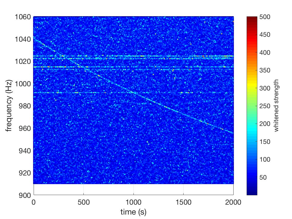
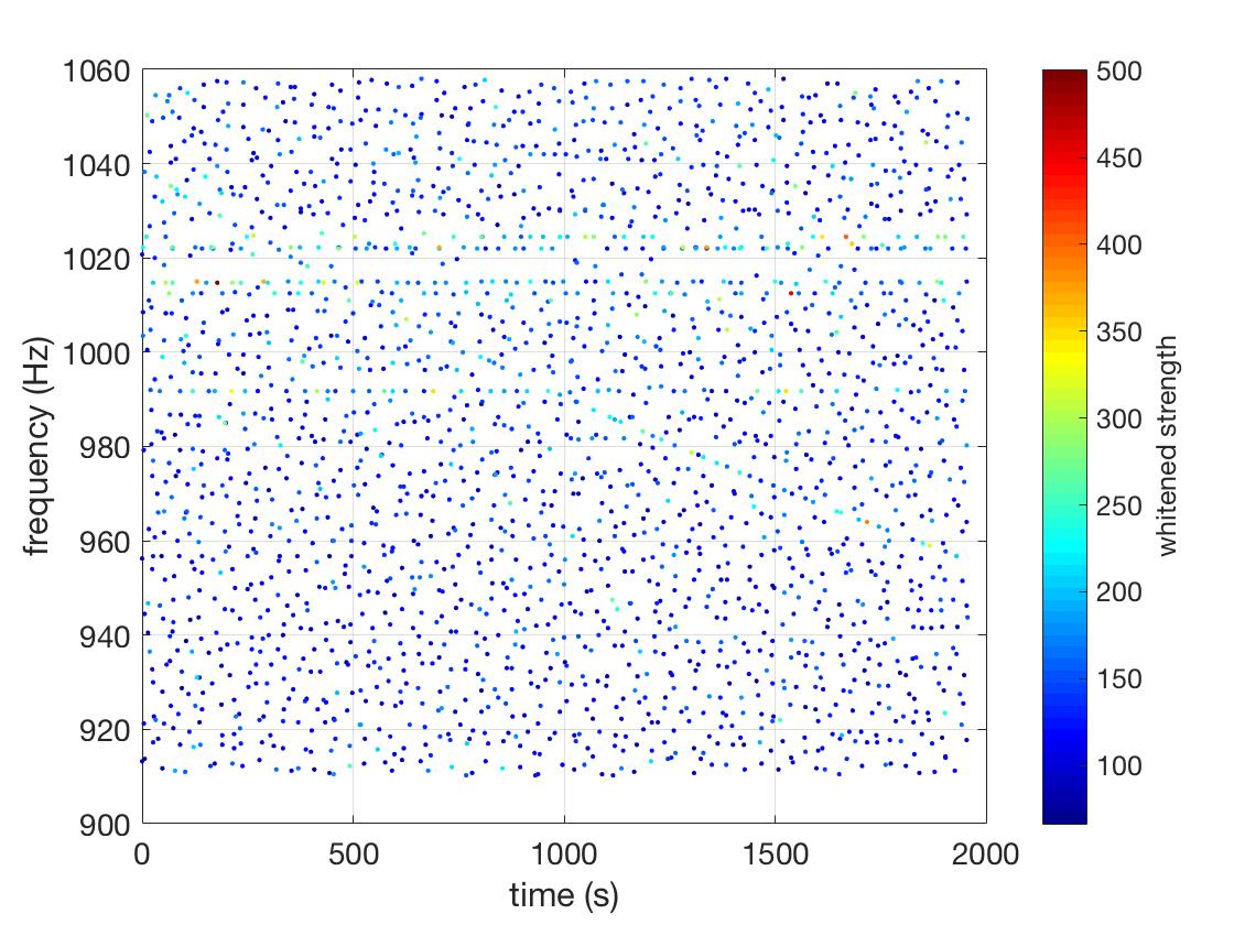
The behavior on which we train the networks is given in Eq. 3, so we first construct a time/frequency map by fast Fourier transforming each chunk of data (interlaced by half and Tukey-windowed). Then, we estimate the noise power spectral density by using an auto-regressive spectrum to whiten the data sfdb_paper . Afterwards we plot the result in the time/frequency plane, as shown in the left panel of Fig. 1. At this level, we must clean the maps, since the CNNs are very sensitive to noise lines. Therefore we zero one or two bins that surround known noise lines Covas:2018oik , and veto any persistent lines in the time/frequency map. This very powerful persistency veto is performed by histogramming the peakmap and projecting it onto the frequency axis. We then compute the median and standard deviation, and if there is a significant increase (more than 1 standard deviation from the median) in the number of peaks in a given frequency bin, we zero all values. This helps to decrease the false alarm probability substantially, while leaving the false dismissal probability unchanged.
Ideally, the more information that we can give to the networks, the better they can learn to identify and distinguish signals from noise. However, there are too many pixels on which to attempt to train the CNNs, so we reduce the resolution of each cleaned time/frequency map in an analogous way as done in mytidis2015sensitivity . We split the time/frequency map into different square blocks and take only the maximum value that appears in each 16 x 16 block, if the value is above a threshold of 2.5; otherwise, we set this value to 0. The size of this box was chosen based on an optimal resolution reduction factor determined in mytidis2015sensitivity . The value 2.5 is equivalent to selecting peaks in the spectrum that are at least 2.5 standard deviations away from the mean level of noise in the map. Selecting a local max and applying a threshold gives us the reduced time/frequency map, constructed in a similar way as the peakmap, a collection of time/frequency peaks that are local maxes above a threshold of 2.5, in Astone:2014esa . But our method of resolution reduction ensures that our maps have the same size, which is necessary for the machine learning to work well. In Fig. 1 we show the before and after resolution-reduction time/frequency maps. From here on, the term “time/frequency maps” will refer to the “reduced time/frequency maps”.
IV Results: Machine learning characterization
For all of these results, we have trained and tested on power-law signals in the time/frequency maps (equation (3)) lasting for s with , Hz, Hz/s, and . All results in this section have been obtained in real O2 Livingston data from science mode periods between 4 January 2017 and 30 March 2017 goetzz , analyzed previously in abbott2019all , using 64000 signal maps and the same number of noise maps generated from Short Fast Fourier Databases T1900140 ; sfdb_paper , though there are only 2000 unique noise maps. Any compact binary system within this time (e.g. GW170104) would have its power spread across many frequency bins, since the spinup of the signal is much greater than the resolution of a frequency bin.
IV.1 Training efficiency
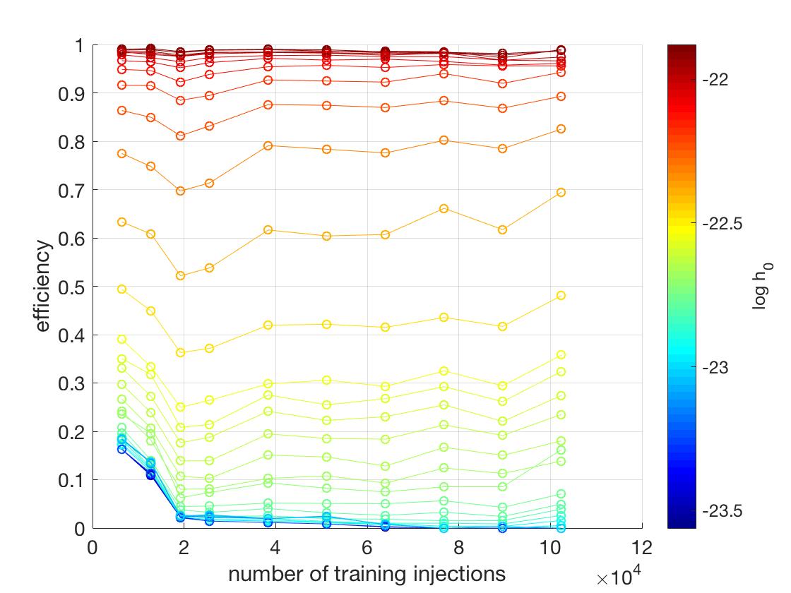
To run a real search, we need to train the CNNs to recognize both signals and noise. However, when we train on noise maps, we have instructed the networks to see these time/frequency maps as not having signals. We would therefore have to throw out this data, so we wish to minimize how much data we need to use for training. Thus we quantify at what point additional training of CNNs no longer adds appreciably to the detection efficiency. Fig. 2 shows a CNN trained with different numbers of injections and noise maps on real data. We apply a threshold on the probability outputted by Eq. (8): , chosen based on the false alarm probability analysis done in section IV.3 . Note that does not imply a detection efficiency of 90%; rather, is our detection statistic. Even for training on injections, we see that the detection efficiencies are comparable to training on injections. This appears to be independent of signal strength. However, when training on fewer injections, we are in fact training on fewer noise maps, which means the false alarm probability is higher. These results depend on which we use, but they offer a guideline for training a single network on a variety of amplitudes.
IV.2 Robustness towards signals not trained on
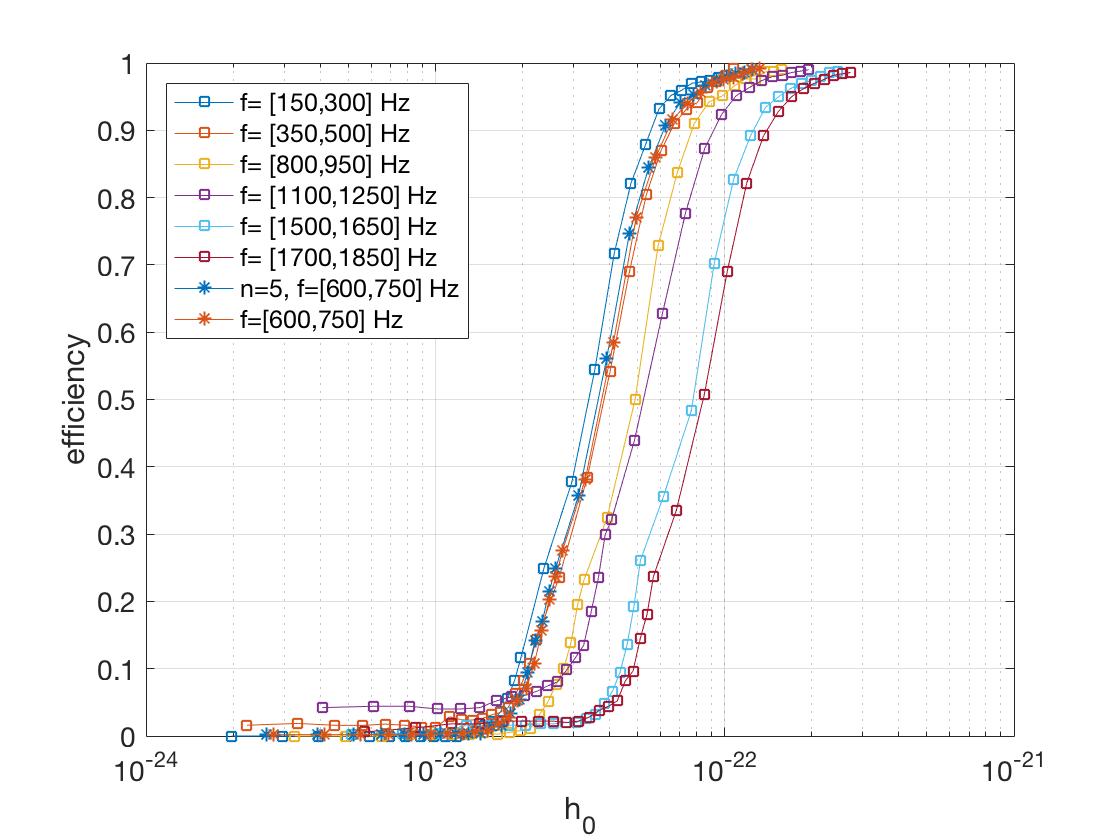
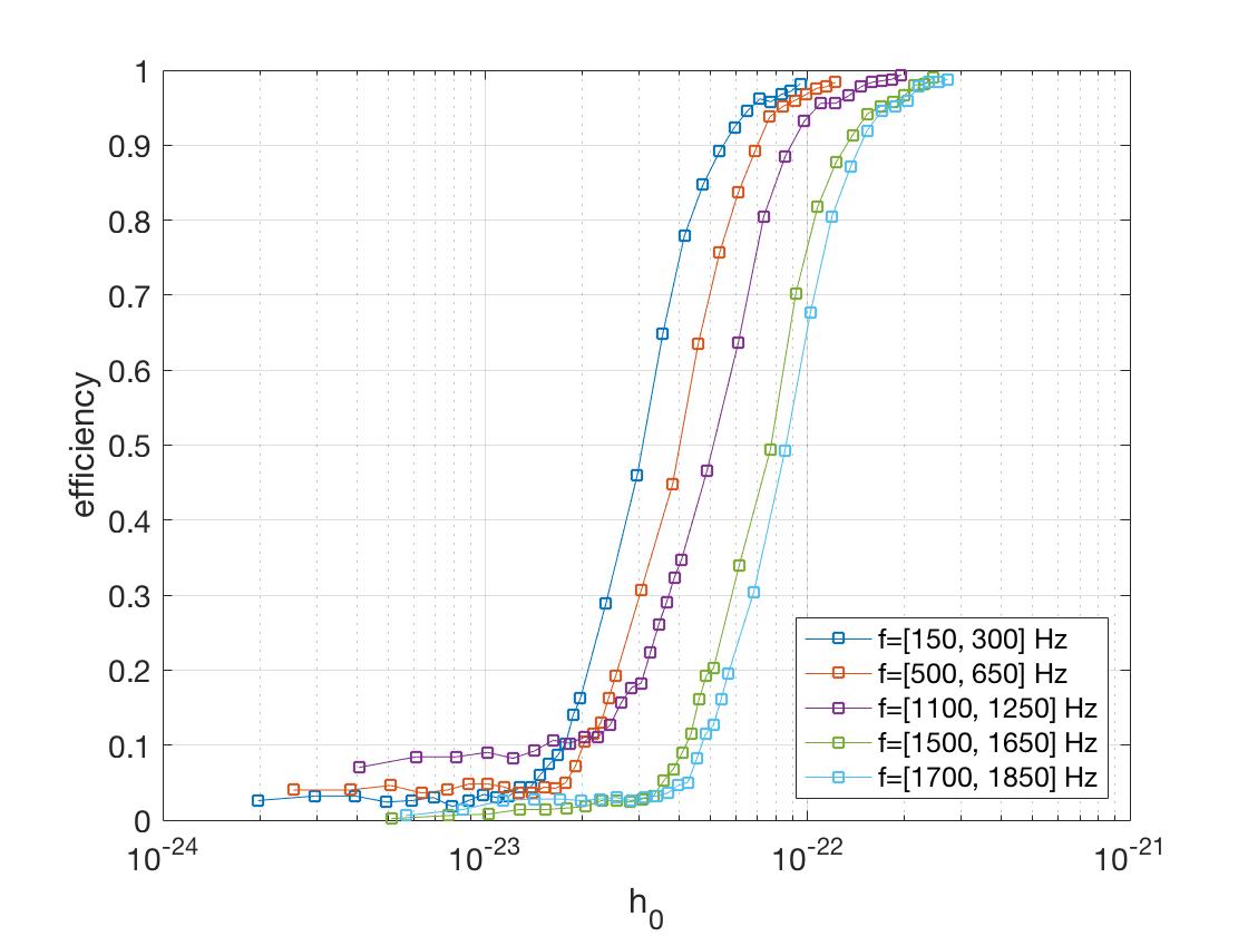
Machine learning methods have become useful because they can be trained to identify certain patterns, and can also generalize to find similar ones, but we must quantify if and how the detection efficiencies will change. The signals we have described thus far have had constant braking indices, which means that the GFH was a strong method to search for them. However, if the braking index varies too quickly in time, the GFH cannot recover the signal, no matter how strong the signal is, because the signal deviates too much from the power law model in Eq. (3). Fig. 3 shows two sets of sensitivity curves for a CNN trained on signals with a braking index of . In the left panel, the curves are the result of testing on injections with fixed braking indices ( or ). The CNNs performed worse at higher frequencies, which is consistent with the sensitivity curve of the LIGO detector. In the right panel, the CNNs were tested on injections with varying braking indices, with variation between /s. In total, this variation corresponds to a change : the GFH cannot detect signals with such large . Comparing both plots in Fig. 3, we see that despite being trained only in the Hz band, the CNNs can detect signals with or without large and have comparable efficiencies across all frequency bands.
IV.3 Impact of on false alarm probability
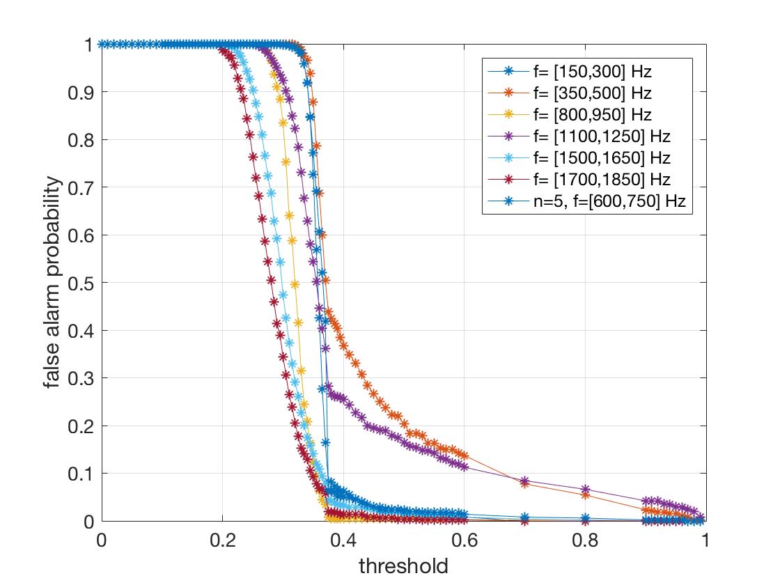
The output of the CNN can be interpreted as a probability that a time/frequency map contains a signal or not. If we wish to decrease the false alarm probability, we can use a threshold that is higher than . To determine an optimal threshold, we test our network on 500 noise maps generated at random times. As shown in Fig. 4, to guarantee a false alarm probability of , we should have depending on the frequency band. We also varied the number of noise maps used for training, and found that 23 days of data (2000 noise maps) was enough to obtain a false alarm probability of at .
IV.4 Error analysis
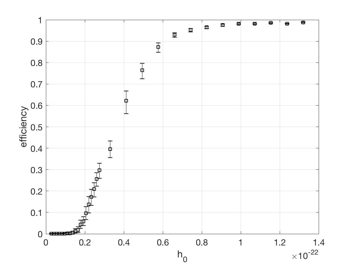
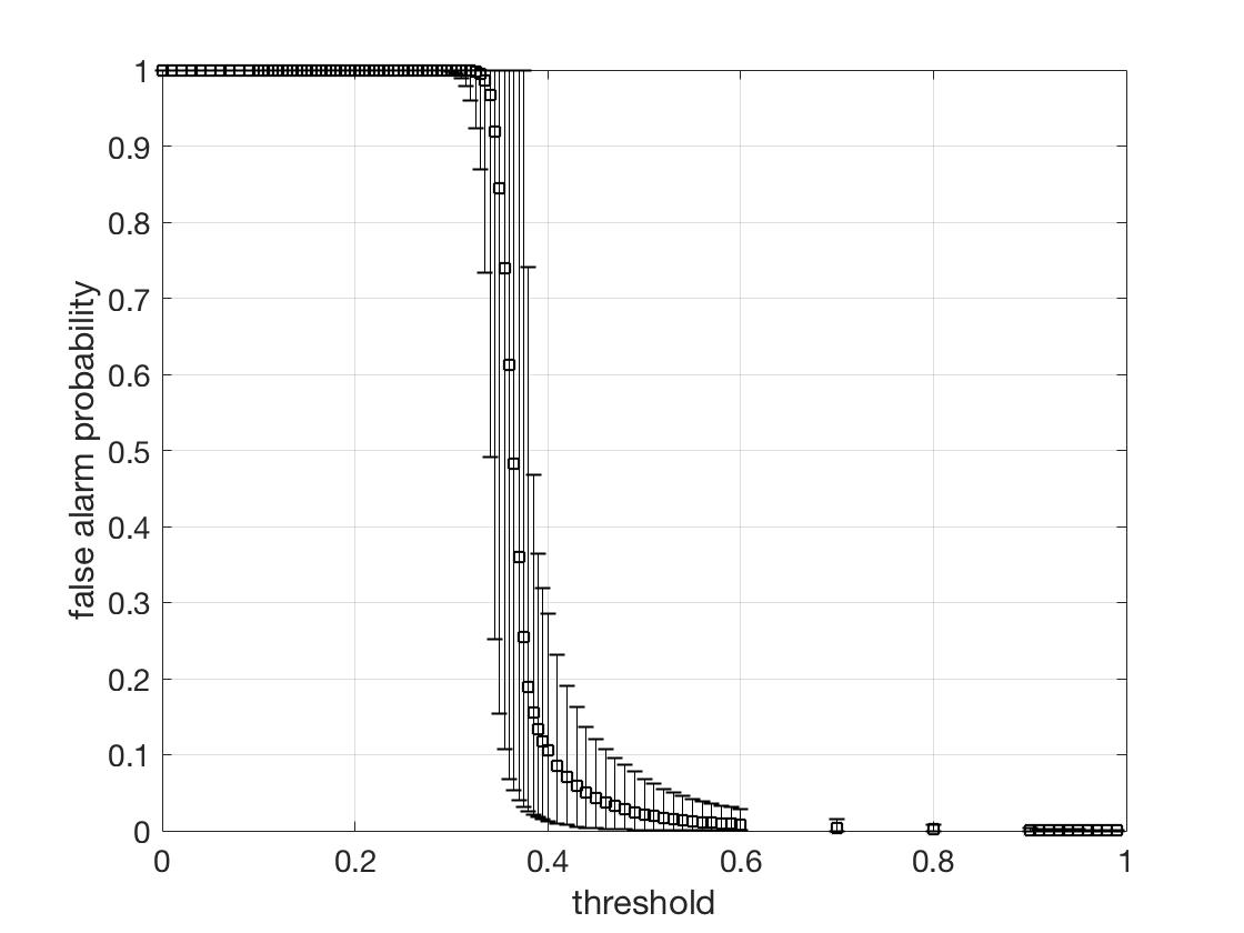
The CNNs operate as a black box: we control the input, the structure of the network and the output. Because of this, there is a good degree of randomness in the possible outputs of the network, meaning that each measurement we make has an associated error. This randomness is caused by the dropout layer, which throws away half of the nodes in the network, and the fact that the network sees randomly shuffled data in different batches in each training session. We therefore train a network 1255 times with the same input data in order to quantify the range of measurements of both detection efficiency and false alarm probability. We discovered that the errors do not obey a binomial distribution for . For the [600, 750] Hz frequency band, we train on 38400 injections and 1200 noise maps. The sensitivity and false alarm probability curves are shown in figure 5.
IV.5 Comparison to Generalized FrequencyHough
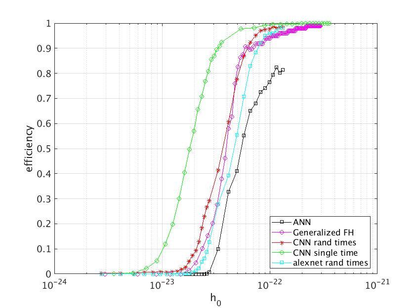
We have compared the detection efficiencies of our CNNs to those of the GFH PhysRevD.98.102004 , to Alexnet CNNs and to ANNs, developed in mytidis2015sensitivity . In Fig. 6, we plot the sensitivity curves for each of these four methods, where we have used for the ANNs and both CNNs. The ANN performs the worst, not even reaching 90% efficiency, while both architectures of CNNs and the GFH achieve similar efficiencies. The CNNs are even slightly more efficient than the GFH at some amplitudes. However, the CNNs cannot perform parameter estimation and the false alarm probabilities are about 100 times greater for both CNNs than for the GFH, see Fig. 4. A “detection” for the GFH is defined as when the parameters and of the loudest candidate in the map are within a distance of 3 bins of the injected signal. For the CNNs, a detection occurs when the returned probability is greater than .
We also show in Fig. 6 the ideal efficiency of a CNN (green curve). This is the best-case scenario because we train and test the CNN at a fixed GPS time, meaning that the CNN learns perfectly the noise structure and hence the false alarm probability is 0. The green curve represents essentially an upper limit on the CNN’s sensitivity. In contrast, the black curve corresponds to the realistic case, where the CNN is affected by the non-stationary noise of the LIGO/Virgo detectors. This result shows that we must be aware of the changing noise in the detector when determining how efficient a CNN will be in detecting power-law signals.
V Search design
We plan to use the CNNs in a real search in order not only to speed up the analysis, but also to probe a portion of the parameter space to which the GFH is not sensitive. It seems that the CNNs are of comparable efficiency to the GFH, so they can be used to quickly analyze time/frequency maps to determine if a signal is present or not. CNNs can analyze a time/frequency map in a microsecond, while the FH and GFH could take minute Astone:2014esa ; PhysRevD.98.102004 . If the map contains a signal, we can then apply the GFH to estimate the parameters of the signal. Moreover, the CNNs are robust towards varying braking indices and different frequency bands with a limited amount of training data. This means that the CNNs can be trained on a small frequency band/time range and then tested across many different frequencies/times.
Once a CNN is trained on injections (at different amplitudes) across 150 Hz and 2000 s maps, for about 22 days of data for a false alarm probability of (which is about 2000 noise maps), we can apply the following procedure for each detector:
-
1.
Load short fast Fourier transform Databases sfdb_paper .
-
2.
Choose appropriate FFT length depending on maximum , create complete time/frequency map and peakmap Astone:2014esa .
-
3.
Clean known noise lines and persistent lines.
-
4.
Reduce resolution by a factor of 16 on each axis.
-
5.
Run CNNs on each reduced time/frequency map.
-
6.
Repeat for each detector’s data. Do coincidences between time/frequency maps that produce triggers.
-
7.
If a trigger remains after the coincidence step, run GFH on the peakmap and obtain parameters of the signal.
-
8.
Perform coincidences between candidates returned by the GFH, follow-up, etc. using methodology described in PhysRevD.98.102004 .
-
9.
Repeat for each 150 Hz/2000 s map.
We must emphasize that if a coincidence occurs between time/frequency maps at the level of the CNNs, the GFH can estimate the parameters of a signal only if it follows a power-law behavior. Otherwise, we can only constrain that the variation in braking index is no more than a certain .
As stated in section IV.1, we cannot test a CNN on the same noise maps on which we train, since the CNN has learned that those maps do not contain a signal. But, if we create different CNNs that are trained and tested on different portions of the data, we can avoid this problem. The logic is the following: suppose we have data for 90 days, and that we need to train a CNN on only 2000 noise maps (23 days of data) to guarantee reasonable false alarm probability/detection efficiency comparable to the GFH. At a minimum, we can train on the first 23 days, and then run an analysis on the last 67 days. Afterwards, we could train on days 24-47, then analyze days 1-23 and 48-90. This would then require the same number of injections, just a doubling of the training time, which takes minutes. The more we repeat this “shifting”, the more times that a different CNN will see the same data.
Since we have shown that the CNNs are robust towards signals in different frequency bands, we should not need injections in each frequency band; rather, it would be sufficient to just train on noise maps across a wide range of frequencies and injection maps in one frequency band. This greatly decreases the computational time required for such an ensemble.
VI Search for a remnant of GW170817
To test our procedure, we ran a search on one week of O2 Livingston and Hanford data after GW170817 to look for a remnant. We split up the search duration in 2000 s time/frequency maps, following the design outlined in the previous section.
Performing this search over one week of data spanning [100,1900] Hz took about 30 minutes. The CNNs took about 2 minutes to analyze the full data set and to generate triggers. Then, the follow-up of these 50 triggers by the GFH took about 15 minutes, when running this follow-up on 14 cores at CNAF-INFN computing center. Finally, the follow-up for the candidate remaining after the GFH took less than a minute.
No significant candidates were found, and the upper limits are consistent with those found in longpmr .
VI.1 Parameter space explored
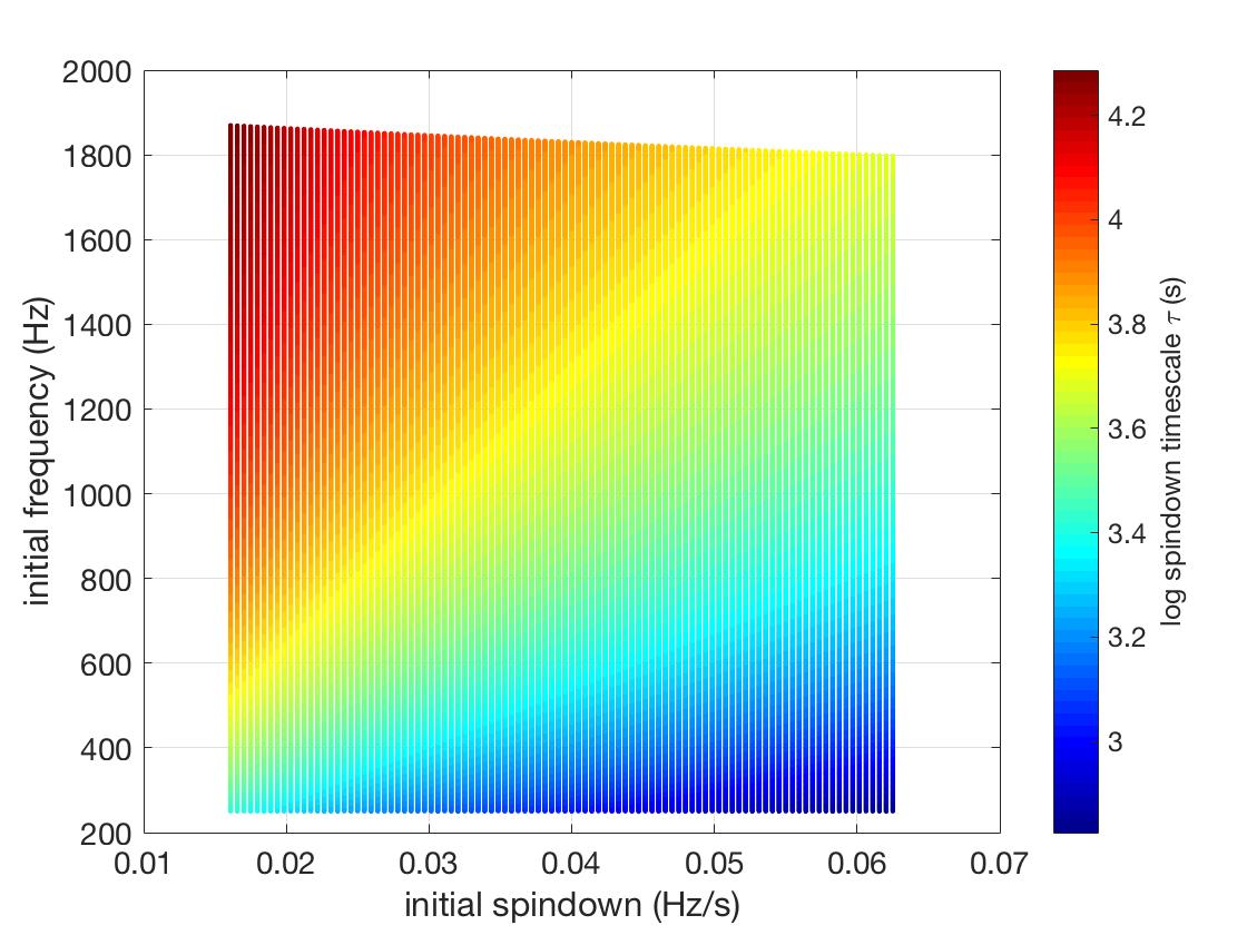
We model the frequency evolution of the signal as a power-law. The initial frequency and spin-down are selected so that a signal will not spin out of the analyzed frequency band during the analysis time. Fig. 7 plots the initial frequencies, spindowns and spindown timescales which meet this criterion for our search configuration, fixing (in general this plot can be created for any braking index). The spindown timescale is colored.
VI.2 Description of search results
Coincidences done in time between the Livingston and Hanford maps analyzed by the CNNs resulted in 50 time/frequency maps having a value of . A grid over was constructed PhysRevD.98.102004 for each of these maps from , in each 150 Hz band between Hz. We then applied the GFH individually to the peakmaps generated at these times (not the maps that the network saw, but the maps constructed by the procedure in Astone:2014esa ). The GFH returned 431 coincident candidates, where a coincidence occurs if the Euclidean distance between candidate parameters in each detector is less than 3 bins. Most candidates had a very low detection statistic, called the critical ratio (CR), defined as:
| (9) |
where is the number count returned by the GFH, and are the mean and standard deviation of the full Hough map, respectively.
We required , corresponding to a false alarm probability of . After applying this threshold, 1 candidate remained (for s). We then use the full Band-Sampled-Data (BSD) piccinibsd follow-up procedure described in PhysRevD.98.102004 . The procedure corrects the peakmaps for the time/frequency evolution of the signal, resulting (theoretically) in a monochromatic signal. is then increased to improve the signal-to-noise ratio and the original FrequencyHough is applied. If the critical ratio of a candidate is less now than before the follow-up, the candidate is vetoed. In each iteration, is doubled. The candidate remained for a few iterations until we used a s, when it was finally vetoed. We therefore conclude that there was no detectable gravitational wave emission from a remnant of GW170817.
VI.3 Upper limits
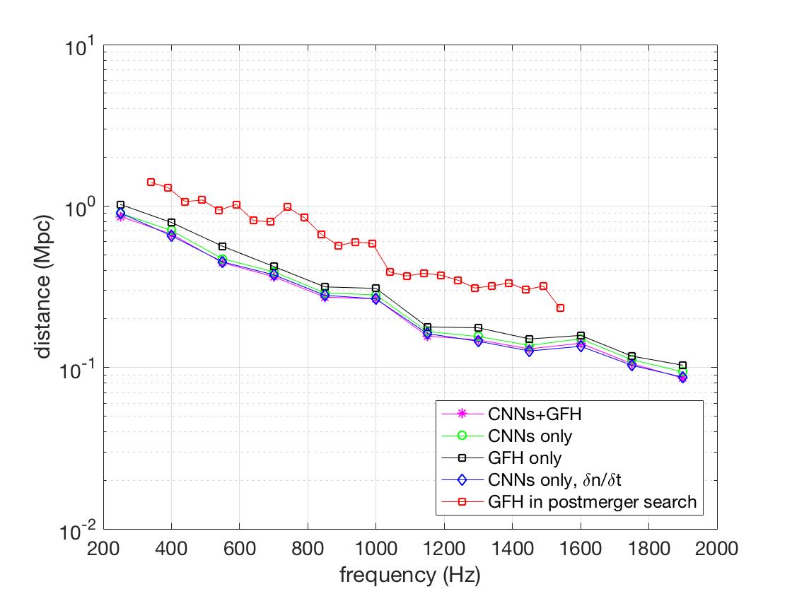
We determine the weakest signals we can see by performing 250 injections, each lasting s, at different amplitudes with parameters uniformly distributed between , Hz, Hz/s, , polarization angle degrees, throughout the entire week after the merger. Another set of injections was also done with /s, analyzed only by the CNNs. A detection is obtained if a candidate returned by the GFH is within 3 bins of the injections and if its , the requirement used in the follow-up in the search. Fig. 8 reports upper limits on distance on a possible power-law signal coming from a remnant of GW170817 at the 50 confidence level. We have plotted five curves: one using the CNNs followed up by the GFH to estimate the parameters of the signal (magenta), one curve using just the CNNs to detect time-varying braking index signals (blue), and three other curves for comparison purposes. The red one is from the original search longpmr , adjusted to be at the confidence level, and the other two curves were obtained by just using the CNNs (green) and GFH (black) to calculate the upper limits. It seems that the previous upper limits are better because the signals were simulated for 2000-16000 s consistent with the search length at longpmr . This should imply an increase of at most in distance reach at higher frequencies, and corresponds to the best sensitivity by about relative to other braking indices at lower frequencies for the GFH, determined by using equation 35 and looking at figure 15 in PhysRevD.98.102004 . Additionally the grid in constructed during the GFH is not optimal for signals of such a short duration, especially at high frequencies, so we are currently investigating ways to improve this grid.
For each curve, we determined the distance reach by assuming a moment of inertia of kg m2, and calculating the maximum allowed ellipticity by energy conservation, as was done in longpmr .
VII Conclusions
We have studied how much we can trust CNNs to detect a gravitational wave signal from isolated neutron stars in real noise. For each data set that a network is given, it is necessary to study how and how much to train, the robustness of the network towards images on which it was not trained, and detection efficiency compared to a traditional algorithm. We have explored the limits of the number of training examples that could be used to train a network, and show that it is possible to achieve comparable detection efficiencies with the limited amount of LIGO/Virgo data we have and expect to obtain in the future, and at a much faster rate than traditional algorithms. We have also successfully applied machine learning to a search of real gravitational wave for a remnant of GW170817, which is the first ever search using CNNs.
In summary:
-
1.
CNNs have comparable efficiencies to the GFH but with a larger false alarm probability depending on the frequency band and how many noise maps we train on.
-
2.
CNNS are at least 5 orders of magnitudes faster than the GFH.
-
3.
Not much training data is necessary to achieve good detection efficiencies. CNNs can therefore be applied quickly to new data in a low-latency way without discarding too much data.
-
4.
Training does not have to cover exhaustively the parameter space =[2.5,7], =[20, 2000] Hz, but we must have an understanding of which value to place on since the false alarm probability may vary in each band.
-
5.
The CNNs are extremely sensitive to lines in the data, to the point where the CNNs will believe that every map that contains a line is a signal, implying a false alarm probability of one. It is therefore crucial to clean the time/frequency maps before giving them to the CNNs.
-
6.
Complicated network architectures do not seem to be needed for this pattern recognition problem. This implies less time necessary for training and less hyperparameters to tune.
-
7.
The place of machine learning in long duration transient analysis is to provide triggers that can be followed up by the GFH, therefore a (not too high, around ) false alarm probability is not a problem.
Future work will include training on previous observing run’s data and testing on new data, in order to avoid using ensembles of CNNs. However, we expect that this will work only when the noise in each observing run does not change too much, which should be the case in future runs. We also plan to experiment with combining two or three detectors’ time/frequency maps into one image, so-called RGB synthesis, that was explored for supernovae in astone2018new . While the efficiency will probably not improve, the false alarm probability should decrease, since noise lines (which we have seen greatly increase the false alarm probability if not removed) are typically not coincident in each detector.
We are also working to estimate and using CNNs. This would allow us to further reduce the computation time necessary for the GFH, since we would not need to loop over all possible braking indices as we did in longpmr . Additionally, if we know , we can correct the time/frequency maps for this behavior before giving them to the GFH.
VIII Acknowledgements
The authors gratefully acknowledge the Italian Istituto Nazionale di Fisica Nucleare (INFN), and the INFN-CNAF for provision of computational resources.
References
- (1) Aasi, J., Abbott, B., Abbott, R., Abbott, T., Abernathy, M., Ackley, K., Adams, C., Adams, T., Addesso, P., Adhikari, R., et al. Advanced ligo. Classical and quantum gravity 32, 7 (2015), 074001.
- (2) Abbott, B., Abbott, R., Abbott, T., Abraham, S., Acernese, F., Ackley, K., Adams, C., Adhikari, R., Adya, V., Affeldt, C., et al. Gwtc-1: A gravitational-wave transient catalog of compact binary mergers observed by ligo and virgo during the first and second observing runs. arXiv preprint arXiv:1811.12907 (2018).
- (3) Abbott, B., Abbott, R., Abbott, T., Abraham, S., Acernese, F., Ackley, K., Adams, C., Adhikari, R., Adya, V., Affeldt, C., et al. All-sky search for continuous gravitational waves from isolated neutron stars using advanced ligo o2 data. Physical Review D 100, 2 (2019), 024004.
- (4) Abbott, B. P., Abbott, R., Abbott, T., Abernathy, M., Acernese, F., Ackley, K., Adams, C., Adams, T., Addesso, P., Adhikari, R., et al. Observation of gravitational waves from a binary black hole merger. Physical review letters 116, 6 (2016), 061102.
- (5) Abbott, B. P., et al. All-sky Search for Periodic Gravitational Waves in the O1 LIGO Data. Phys. Rev. D96, 6 (2017), 062002.
- (6) Abbott, B. P., et al. Gw170817: Observation of gravitational waves from a binary neutron star inspiral. Phys. Rev. Lett. 119 (Oct 2017), 161101.
- (7) Abbott, B. P., et al. Search for gravitational waves from a long-lived remnant of the binary neutron star merger GW170817. The Astrophysical Journal 875, 2 (apr 2019), 160.
- (8) Acernese, F., Agathos, M., Agatsuma, K., Aisa, D., Allemandou, N., Allocca, A., Amarni, J., Astone, P., Balestri, G., Ballardin, G., et al. Advanced virgo: a second-generation interferometric gravitational wave detector. Classical and Quantum Gravity 32, 2 (2014), 024001.
- (9) Alford, M. G., and Schwenzer, K. Gravitational wave emission from oscillating millisecond pulsars. Monthly Notices of the Royal Astronomical Society 446, 4 (2014), 3631–3641.
- (10) Archibald, R., Gotthelf, E., Ferdman, R., Kaspi, V., Guillot, S., Harrison, F., Keane, E., Pivovaroff, M., Stern, D., Tendulkar, S., et al. A high braking index for a pulsar. The Astrophysical Journal Letters 819, 1 (2016), L16.
- (11) Astone, P., Cerdá-Durán, P., Di Palma, I., Drago, M., Muciaccia, F., Palomba, C., and Ricci, F. New method to observe gravitational waves emitted by core collapse supernovae. Physical Review D 98, 12 (2018), 122002.
- (12) Astone, P., Colla, A., D’Antonio, S., Frasca, S., and Palomba, C. Method for all-sky searches of continuous gravitational wave signals using the frequency-Hough transform. Phys. Rev. D90, 4 (2014), 042002.
- (13) Astone, P., et al. Codes to create sfdbs and o2 used time segments. Tech. Rep. LIGO-T1900140, 2019.
- (14) Astone, P., Frasca, S., and Palomba, C. The short fft database and the peak map for the hierarchical search of periodic sources. Classical and Quantum Gravity 22, 18 (2005), S1197.
- (15) Baiotti, L., and Rezzolla, L. Binary neutron star mergers: a review of Einstein’s richest laboratory. Rept. Prog. Phys. 80, 9 (2017), 096901.
- (16) Bauswein, A., and Janka, H.-T. Measuring neutron-star properties via gravitational waves from neutron-star mergers. Physical review letters 108, 1 (2012), 011101.
- (17) Clark, C., Pletsch, H., Wu, J., Guillemot, L., Camilo, F., Johnson, T., Kerr, M., Allen, B., Aulbert, C., Beer, C., et al. The braking index of a radio-quiet gamma-ray pulsar. The Astrophysical journal letters 832, 1 (2016), L15.
- (18) Covas, P., et al. Identification and mitigation of narrow spectral artifacts that degrade searches for persistent gravitational waves in the first two observing runs of Advanced LIGO. Phys. Rev. D97, 8 (2018), 082002.
- (19) Dreissigacker, C., Sharma, R., Messenger, C., Zhao, R., and Prix, R. Deep-learning continuous gravitational waves. arXiv preprint arXiv:1904.13291 (2019).
- (20) et al., B. A. All-sky search for continuous gravitational waves from isolated neutron stars using advanced ligo o2 data. arXiv preprint arXiv:1903.01901 (2019).
- (21) Gabbard, H., Williams, M., Hayes, F., and Messenger, C. Matching matched filtering with deep networks for gravitational-wave astronomy. Physical review letters 120, 14 (2018), 141103.
- (22) Gebhard, T. D., Kilbertus, N., Harry, I., and Schölkopf, B. Convolutional neural networks: a magic bullet for gravitational-wave detection? arXiv preprint arXiv:1904.08693 (2019).
- (23) George, D., and Huerta, E. Deep learning for real-time gravitational wave detection and parameter estimation: Results with advanced ligo data. Physics Letters B 778 (2018), 64–70.
- (24) George, D., and Huerta, E. Deep neural networks to enable real-time multimessenger astrophysics. Physical Review D 97, 4 (2018), 044039.
- (25) Goetz, E., and LSC/Virgo. Segments used for creating standard sfts in o2 data. Tech. Rep. LIGO-T1900085.
- (26) Hamil, O., Stone, J. R., Urbanec, M., and Urbancova, G. Braking index of isolated pulsars. Physical Review D 91, 6 (2015), 063007.
- (27) Jaranowski, P., Królak, A., and Schutz, B. F. Data analysis of gravitational-wave signals from spinning neutron stars: The signal and its detection. Phys. Rev. D58 (1998), 063001.
- (28) Keitel, D., Woan, G., Pitkin, M., Schumacher, C., Pearlstone, B., Riles, K., Lyne, A. G., Palfreyman, J., Stappers, B., and Weltevrede, P. First search for long-duration transient gravitational waves after glitches in the vela and crab pulsars. arXiv preprint arXiv:1907.04717 (2019).
- (29) Lasky, P. D., Leris, C., Rowlinson, A., and Glampedakis, K. The braking index of millisecond magnetars. The Astrophysical Journal Letters 843, 1 (2017), L1.
- (30) Miller, A., Astone, P., D’Antonio, S., Frasca, S., Intini, G., La Rosa, I., Leaci, P., Mastrogiovanni, S., Muciaccia, F., Palomba, C., Piccinni, O. J., Singhal, A., and Whiting, B. F. Method to search for long duration gravitational wave transients from isolated neutron stars using the generalized frequency-hough transform. Phys. Rev. D 98 (Nov 2018), 102004.
- (31) Muciaccia, F. Using deep convolutional neural networks to build a low-latency classifier to trigger the detection of long gravitational wave transients.
- (32) Mytidis, A., Panagopoulos, A. A., Panagopoulos, O. P., Miller, A., and Whiting, B. Sensitivity study using machine learning algorithms on simulated -mode gravitational wave signals from newborn neutron stars. Phys. Rev. D 99 (Jan 2019), 024024.
- (33) Oliver, M., Keitel, D., and Sintes, A. M. Adaptive transient hough method for long-duration gravitational wave transients. Physical Review D 99, 10 (2019), 104067.
- (34) Owen, B. J., Lindblom, L., Cutler, C., Schutz, B. F., Vecchio, A., and Andersson, N. Gravitational waves from hot young rapidly rotating neutron stars. Phys. Rev. D58 (1998), 084020.
- (35) Piccinni, O., Astone, P., D’Antonio, S., Frasca, S., Intini, G., Leaci, P., Mastrogiovanni, S., Miller, A., Palomba, C., and Singhal, A. A new data analysis framework for the search of continuous gravitational wave signals. Classical and Quantum Gravity 36, 1 (2018), 015008.
- (36) Prix, R., Giampanis, S., and Messenger, C. Search method for long-duration gravitational-wave transients from neutron stars. Physical Review D 84, 2 (2011), 023007.
- (37) Riles, K. Recent searches for continuous gravitational waves. Modern Physics Letters A 32, 39 (2017), 1730035.
- (38) Sarin, N., Lasky, P. D., Sammut, L., and Ashton, G. X-ray guided gravitational-wave search for binary neutron star merger remnants. Physical Review D 98, 4 (2018), 043011.
- (39) Shapiro, S. L., and Teukolsky, S. A. Black holes, white dwarfs, and neutron stars: The physics of compact objects. Wiley, New York, 1983.
- (40) Sun, L., and Melatos, A. Application of hidden markov model tracking to the search for long-duration transient gravitational waves from the remnant of the binary neutron star merger gw170817. Physical Review D 99, 12 (2019), 123003.
- (41) Thrane, E., et al. Long gravitational-wave transients and associated detection strategies for a network of terrestrial interferometers. Phys. Rev. D83 (2011), 083004.
- (42) Thrane, E., Mandic, V., and Christensen, N. Detecting very long-lived gravitational-wave transients lasting hours to weeks. Physical Review D 91, 10 (2015), 104021.