LCA: Loss Change Allocation for
Neural Network Training

Abstract

Neural networks enjoy widespread use, but many aspects of their training, representation, and operation are poorly understood. In particular, our view into the training process is limited, with a single scalar loss being the most common viewport into this high-dimensional, dynamic process. We propose a new window into training called Loss Change Allocation (LCA), in which credit for changes to the network loss is conservatively partitioned to the parameters. This measurement is accomplished by decomposing the components of an approximate path integral along the training trajectory using a Runge-Kutta integrator. This rich view shows which parameters are responsible for decreasing or increasing the loss during training, or which parameters “help” or “hurt” the network’s learning, respectively. LCA may be summed over training iterations and/or over neurons, channels, or layers for increasingly coarse views. This new measurement device produces several insights into training. (1) We find that barely over 50% of parameters help during any given iteration. (2) Some entire layers hurt overall, moving on average against the training gradient, a phenomenon we hypothesize may be due to phase lag in an oscillatory training process. (3) Finally, increments in learning proceed in a synchronized manner across layers, often peaking on identical iterations.

1 Introduction

In the common stochastic gradient descent (SGD) training setup, a parameterized model is iteratively updated using gradients computed from mini-batches of data chosen from some training set. Unfortunately, our view into the high-dimensional, dynamic training process is often limited to watching a scalar loss quantity decrease over time. There has been much research attempting to understand neural network training, with some work studying geometric properties of the objective function [7, 20, 28, 24, 21], properties of whole networks and individual layers at convergence [4, 7, 15, 35], and neural network training from an optimization perspective [30, 4, 5, 3, 19]. This body of work in aggregate provides rich insight into the loss landscape arising from typical combinations of neural network architectures and datasets. Literature on the dynamics of the training process itself is more sparse, but a few salient works examine the learning phase through the diagonal of the Hessian, mutual information between input and output, and other measures [1, 25, 14].

In this paper we propose a simple approach to inspecting training in progress by decomposing changes in the overall network loss into a per-parameter Loss Change Allocation or LCA. The procedure for computing LCA is straightforward, but to our knowledge it has not previously been employed for investigating network training. We begin by defining this measure in more detail, and then apply it to reveal several interesting properties of neural network training. Our contributions are as follows:

1. We define the Loss Change Allocation as a per-parameter, per-iteration decomposition of changes to the overall network loss (Section 2). Exploring network training with this measurement tool uncovers the following insights.

2. Learning is very noisy, with only slightly over half of parameters helping to reduce loss on any given iteration (Section 3).

3. Some entire layers consistently drift in the wrong direction during training, on average moving against the gradient. We propose and test an explanation that these layers are slightly out of phase, lagging behind other layers during training (Section 4).

4. We contribute new evidence to suggest that the learning progress is, on a microscopic level, synchronized across layers, with small peaks of learning often occurring at the same iteration for all layers (Section 5).

2 The Loss Change Allocation approach

Figure 1: (a) Illustration of this paper’s method on a toy two-dimensional loss surface. We allocate credit for changes to the model’s training loss to individual parameters (b) $\theta~{}\mathrm{dim\mbox{-}1}$ and (c) $\theta~{}\mathrm{dim\mbox{-}2}$ by multiplying parameter motion with the corresponding individual component of the gradient of the training set. This partitions changes to the loss into individual Loss Change Allocation (LCA) components allows us to measure which parameters learn at each timestep, providing a rich view into the training process. In the example depicted, although both parameters move, the second parameter captures all the credit, as only its component of the gradient is non-zero.

We begin by defining the Loss Change Allocation approach in more detail. Consider a parameterized training scenario where a model starts at parameter value $\theta_{0}$ and ends at parameter value $\theta_{T}$ after training. The training process entails traversing some path $P$ along the surface of a loss landscape from $\theta_{0}$ to $\theta_{T}$. There are several loss landscapes one might consider; in this paper we analyze the training process, so we measure motion along the loss with respect to the entire training set, here denoted simply $L(\theta)$. We analyze the loss landscape of the training set instead of the validation set because we aim to measure training, not training confounded with issues of memorization vs. generalization (though the latter certainly should be the topic of future studies).

The approach in this paper derives from a straightforward application of the fundamental theorem of calculus to a path integral along the loss landscape:

$$L(\theta_{T})-L(\theta_{0})=\int_{C}\langle\nabla_{\theta}L(\theta),d\theta\rangle$$ (1)

where $C$ is any path from $\theta_{0}$ to $\theta_{T}$ and $\langle\cdot{,}\cdot\rangle$ is the dot product. This equation states that the change in loss from $\theta_{0}$ to $\theta_{T}$ may be calculated by integrating the dot product of the loss gradient and parameter motion along a path from $\theta_{0}$ to $\theta_{T}$. Because $\nabla_{\theta}L(\theta)$ is the gradient of a function and thus is a conservative field, any path from $\theta_{0}$ to $\theta_{T}$ may be used; in this paper we consider the path taken by the optimizer during the course of training. We may approximate this path integral from $\theta_{0}$ to $\theta_{T}$ by using a series of first order Taylor approximations along the training path. If we index training steps by $t\in[0,1,...,T]$, the first order approximation for the change in loss during one step of training is the following, rewritten as a sum of its individual components:

$$L(\theta_{t+1})-L(\theta_{t}) \approx\langle\nabla_{\theta}L(\theta_{t}),~{}\theta_{t+1}-\theta_{t}\rangle$$ (2)

$$=\sum_{i=0}^{K-1}(\nabla_{\theta}L(\theta_{t}))^{(i)}(\theta_{t+1}^{(i)}-\theta_{t}^{(i)})\vcentcolon=\sum_{i=0}^{K-1}A_{t,i}$$ (3)

where $\nabla_{\theta}L(\theta_{t})$ represents the gradient of the loss of the whole training set w.r.t. $\theta$ evaluated at $\theta_{t}$, $v^{(i)}$ represents the $i$-th element of a vector $v$, and the parameter vector $\theta$ contains $K$ elements. Note that while we evaluate model learning by tracking progress along the training set loss landscape $L(\theta)$, training itself is accomplished using stochastic gradient approaches in which noisy gradients from mini-batches of data drive parameter updates via some optimizer like SGD or Adam. As shown in Equation 3, the difference in loss produced by one training iteration $t$ may be decomposed into $K$ individual Loss Change Allocation, or LCA, components, denoted $A_{t,i}$. These $K$ components represent the LCA for a single iteration of training, and over the course of $T$ iterations of training we will collect a large $T\times K$ matrix of $A_{t,i}$ values.

The total loss over the course of training will often decrease, and the above decomposition allows us to allocate credit for loss decreases on a per-parameter, per-timestep level. Intuitively, when the optimizer increases the value of a parameter and its component of the gradient on the whole training set is negative, the parameter has a negative LCA and is “helping” or “learning”. Positive LCA is “hurting” the learning process, which may result from several causes: a noisy mini-batch with the gradient of that step going the wrong way, momentum, or a step size that is too large for a curvy or rugged loss landscape as seen in [14, 32]. If the parameter has a non-zero gradient but does not move, it does not affect the loss. Similarly, if a parameter moves but has zero gradient, it does not affect the loss. The sum of the $K$ components is the overall change in loss at that iteration. Figure 1 depicts a toy example using two parameters. Throughout the paper we use “helping” to indicate negative LCA (a contribution to the reduction of total loss), and “hurting” for positive LCA.

An important property of this decomposition is that it is grounded: the sum of individual components equals the total change in loss, and each contribution has the same fundamental units as the loss overall (e.g. nats or bits in the case of cross-entropy). This is in contrast to approaches that measure quantities like parameter motion or approximate elements of the Fisher information (FI) [16, 1], which also produce per-parameter measurements but depend heavily on the parameterization chosen. For example, the FI metric is sensitive to scale (e.g. multiply one relu layer weights by 2 and next by 0.5: loss stays the same but FI of each layer changes and total FI changes). Further, LCA has the benefit of being signed, allowing us to make measurements and interpretations when training goes backwards (Sections 3 and 4).

Ideally, summing up the $K$ components should equal $L(\theta_{t+1})-L(\theta_{t})$. In practice, the first order Taylor approximation is often inaccurate due to the curvature of the loss landscape. We can improve on our LCA approximation from Equation 2 by replacing $\nabla_{\theta}L(\theta_{t})$ with $\frac{1}{6}(\nabla_{\theta}L(\theta_{t})+4\nabla_{\theta}L(\frac{1}{2}\theta_{t}+\frac{1}{2}\theta_{t+1})+\nabla_{\theta}L(\theta_{t+1}))$, with the $(1,4,1)$ coefficients coming from the fourth-order Runge–Kutta method (RK4) [23, 17] or equivalently from Simpson’s rule [31]. Using a midpoint gradient doubles computation but shrinks accumulated error drastically, from first order to fourth order. If the error is still too large, we can halve the step size with composite Simpson’s rule by calculating gradients at $\frac{3}{4}\theta_{t}+\frac{1}{4}\theta_{t+1}$ and $\frac{1}{4}\theta_{t}+\frac{3}{4}\theta_{t+1}$ as well. We halve the step size until the absolute error of change in loss per iteration is less than 0.001, and we ensure that the cumulative error at the end of training is less than 1%. First order and RK4 errors can be found in Table S1 in Supplementary Information. Note that the approach described may be applied to any parameterized model trained via gradient descent, but for the remainder of the paper we assume the case of neural network training.

Figure 2: Frames from an animation of the learning process for two training runs. (left) The 1st layer of an MNIST–FC (full shape is 100$\times$784, but only the upper left quarter is shown for better clarity). (right) The 2nd convolutional layer of an MNIST–LeNet (full shape is 40$\times$20 of 5$\times$5 blocks; only upper left quarter is shown). Each pixel represents one parameter. The LeNet layer shows 5$\times$5 grids representing each filter, laid out by input channels (columns) and output channels (rows). Parameters that help (decrease the loss) at a given time are shown as shades of green. Parameters that hurt (increase the loss) are shown as shades of red. Larger magnitudes of LCA are darker and white indicates zero LCA. Iteration 20 is partly through the main drop in loss, and 220 is one full epoch. In MNIST–FC, we can see clusters spaced at intervals of 28 pixels, because these parameters connect to the flattened MNIST images. Learning is strongest in early iterations with mostly negative LCA, remains strong for many iterations but with more variance in LCA across parameters, and has greatly diminished by iteration 220, where much of learning is complete. The complete animations may be viewed at: %JBY:␣removed␣vvv␣this␣because␣the␣visualization␣is␣fine␣without␣it.%Within␣each␣network,␣the␣same␣color␣and␣shade␣represents␣the␣same␣LCA␣value␣across␣the␣different␣iterations.%White␣bands␣between␣clusters␣correspond␣to␣parameters␣that␣do␣not␣learn␣because␣their␣input␣pixels␣are␣never␣non-zero␣(a␣peculiarity␣of␣MNIST).https://youtu.be/xcnoRnoVyXQ and https://youtu.be/EY3LoXmdkYU.

2.1 Experiments

We employ the LCA approach to examine training on two tasks: MNIST and CIFAR-10, with architectures including a 3-layer fully connected (FC) network and LeNet [18] on MNIST, and AllCNN [29] and ResNet-20 [9] on CIFAR-10. Throughout this paper we refer to training runs as “dataset–network”, e.g., MNIST–FC, MNIST–LeNet, CIFAR–AllCNN, CIFAR–ResNet, followed by further configuration details (such as the optimizer) when needed.

For each dataset–network configuration, we train with both SGD and Adam optimizers, and conduct multiple runs with identical hyperparameter settings. Momentum of 0.9 is used for all SGD runs, except for one set of “no-momentum” MNIST–FC experiments. Learning rates are manually chosen between 0.001 to 0.5. See Section S7 in Supplementary Information for more details on architectures and hyperparameters. We also make our code available at https://github.com/uber-research/loss-change-allocation. Note that we use standard network architectures to demonstrate use cases of our tool; we strive for simplicity and interpretability of results rather than state-of-the-art performance. Thus we do not incorporate techniques such as L2 regularization, data augmentation, and learning rate decay. Since our method requires calculating gradients of the loss over the entire training set, it is considerably slower than the regular training process, but remains tractable for small to medium models; see Section S8 for more details on computation.

2.2 Direct visualization

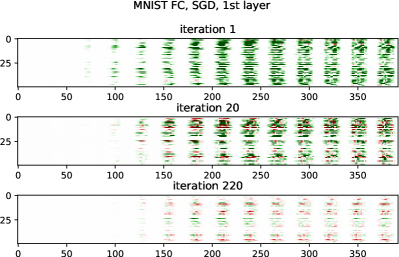
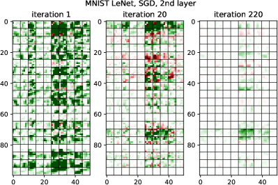
We calculate LCA for every parameter at every iteration and animate the LCA values through all the iterations in the whole training process. Figure 2 shows snapshots of frames from the video visualization. In such videos, we arrange parameters first by layer and then for each layer as two-dimensional matrices (1-D vectors for biases), and overlay LCA values as a heatmap. This animation enables a granular view of the training process.

We can also directly visualize each parameter versus time, granting each parameter its own training curve. We can optionally aggregate over neurons, channels, layers, etc. (see Section S2 for examples). A benefit of these visualizations is that they convey a large volume of data directly to the viewer, surfacing subtle patterns and bugs that can be further investigated. Observed patterns also suggest more quantitative metrics that surface traits of training. The rest of the paper is dedicated to such metrics and traits.

Figure 3: (a) Visualization of the percentage of parameters that helped, hurt, or had zero effect through training, overlaid with the loss curve of that run. (b) The distribution of helping and hurting LCA (zeros ignored) over the entire training, zoomed in to ignore 1% of tails. (c) Average percent of weights helping for each layer in network, curiously near 50% for all. (d) Histogram of the fraction of iterations each weight helped, showing that most weights swing back and forth between helping and hurting evenly. In every column the first row is MNIST–FC and second row CIFAR–ResNet, both trained with SGD. Notable facts: MNIST–FC shows a significant percent of weights with zero effect. Because MNIST has pixels that are never on, any first layer weights connected to those pixels cannot help or hurt. CIFAR–ResNet exhibits barely over 50% of parameters helping over the course of training, even during the period of significantly learning (loss reduction) from iteration 0 to 2000. Averaged over the entire run, only 50.66% of parameters helped (see Table 1). Note that in both runs we can see that in the earliest iterations, the percent of weights helping is higher, but only slightly.

3 Learning is very noisy

Although it is a commonly held view that the inherent noise in SGD-based neural network training exists and is even considered beneficial [15], this noise is often loosely defined as a deviation in gradient estimation. While the minibatch gradient serves as as a suggested direction for parameter movement, it is still one step away from the actual impact on decreasing loss over the whole training set, which LCA represents precisely. By aggregating a population of per-parameter, per-iteration LCAs along different axes, we present numerical results that shed light into the noisy learning behavior. We find it surprising that on average almost half of parameters are hurting in every training iteration. Moreover, each parameter, including ones that help in total, hurt almost half of the time.

Barely over 50% of parameters help during training.

Table 1: Percentage of helping parameters (ignoring those with zero LCA) for various networks and optimizers, averaged across all iterations and 3 independent runs per per configuration.

	MNIST-FC, mom=0	MNIST-FC	MNIST-LeNet	CIFAR-ResNet	CIFAR-AllCNN
SGD	$53.72\pm 0.05$	$57.79\pm 0.16$	$53.97\pm 0.48$	$50.66\pm 0.14$	$51.09\pm 0.23$
Adam	N/A	$55.82\pm 0.09$	$51.77\pm 0.21$	$50.30\pm 0.004$	$50.19\pm 0.01$

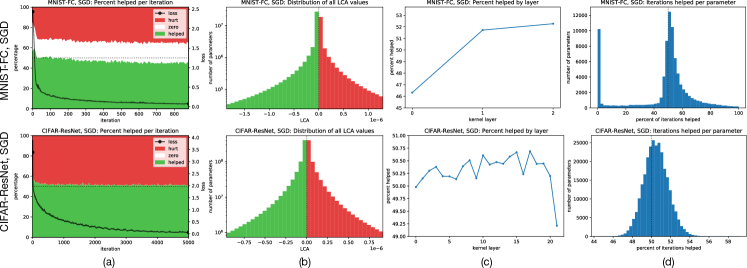
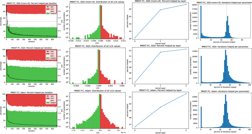
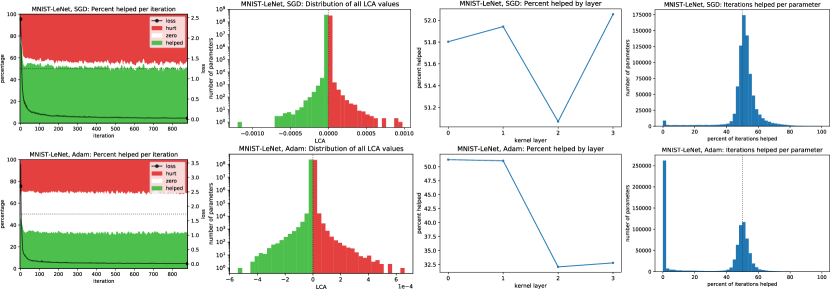
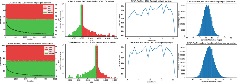
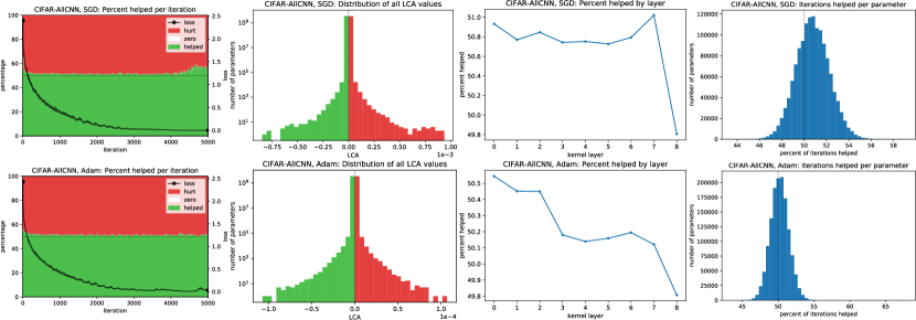
According to our definition, for each iteration of training, parameters can help, hurt, or not impact the overall loss. With that in mind, we count the number of parameters that help, hurt, or neither, across all training iterations and for various networks; two examples of networks are shown in Figure 3 (all other networks shown in Section S3). The data show that in a typical training iteration, close to half of parameters are helping and close to half are hurting! This ratio is slightly skewed towards helping in early iterations but stays fairly constant during training. Averaged across all iterations, the percentage of helping parameters for various network configurations is reported in Table 1. We see that it varies within a small range of 50% to 58%, with CIFAR networks even tighter at 50% to 51%. This observation also holds true when we look at each layer separately in a network; Figure 3(c) shows that all layers have similar ratios of helpful parameters.

Parameters alternate helping.

Now that we can tell if each parameter is “helpful”, “hurtful”, or “neither”, we wonder if parameters predictably stay in the same category throughout training. In other words, is there a consistent elite group of parameters that always help? When we measure the percentage of helpful iterations per parameter throughout a training run, histograms in Figure 3(d) show that parameters help approximately half of the time, and therefore the training of a network is achieved by parameters alternating to make helpful contribution to the loss.

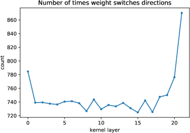
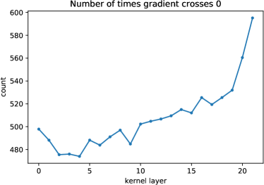
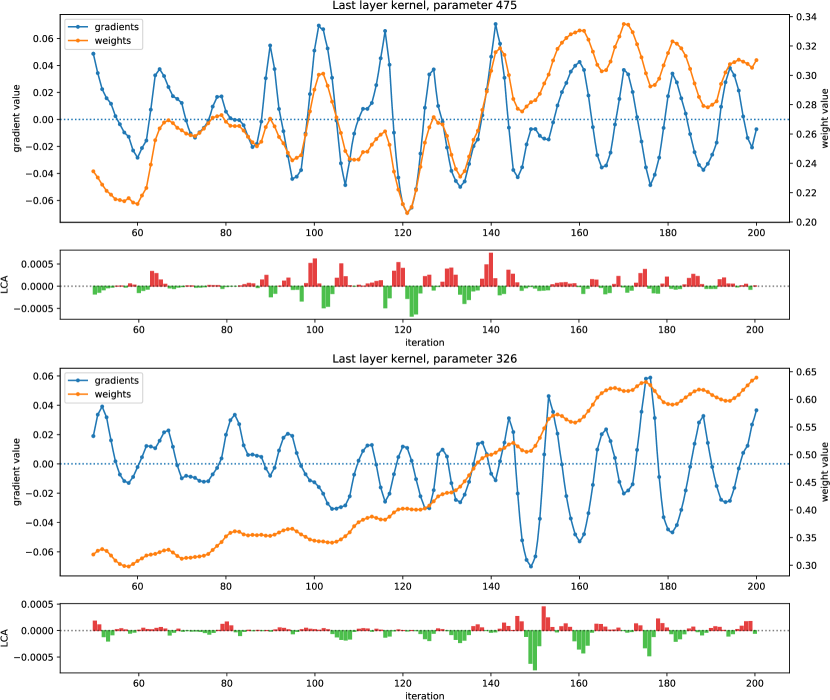
Additionally, we can measure the oscillations of individual parameters. Figure S7 shows a high number of oscillations in weight movement for CIFAR–ResNet on SGD: on average, weight movements change direction once every 6.7 iterations, and gradients change signs every 9.5 iterations. Section S3 includes these measures for all networks, as well as detailed views in Figure S8 suggesting that many of these oscillations happen around local minima. While oscillations have been previously observed for the overall network [32, 14], thanks to LCA, we’re able to more precisely quantify the individual and net effects of these oscillations. As we’ll see in Section 4, we can also use LCA to identify when a network is damaged not by oscillations themselves, but by their precise phase.

Noise persists across various hyperparameters.

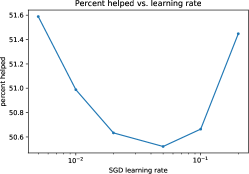
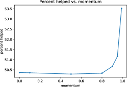
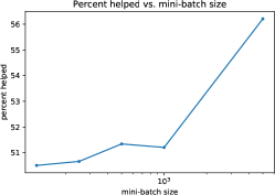
Changing the learning rate, momentum, or batch size (within reasonable ranges such that the network still trains well) only have a slight effect on the percent of parameters helping. See Section S3 for a set of experiments on CIFAR–ResNet with SGD, where percent helped always stays within 50.3% to 51.6% for reasonable hyperparameters.

Learning is heavy-tailed.

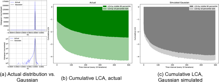
A reasonable mental model of the distribution of LCA might be a narrow Gaussian around the mean. However, we find that this is far from reality. Instead, the LCA of both helping and hurting parameters follow a heavy-tailed distribution, as seen in Figure 3(b). Figure S10 goes into more depth in this direction, showing that contributions from the tail are about three times larger than would be expected if learning were Gaussian distributed. More precisely, a better model of LCA would be the Weibull distribution with $k<1$. The measurements suggest that the view of learning as a Wiener process [25] should be refined to reflect the heavy tails.

4 Some layers hurt overall

Although our method is used to study low-level, per-parameter LCA, we can also aggregate these over higher level breakdowns for different insights; individually there is a lot of noise, but on the whole, the network learns. The behavior of individual layers during learning has been of interest to many researchers [35, 22], so a simple and useful aggregation is to sum LCA over all parameters within each layer and sum over all time, measuring how much each layer contributes to total learning.

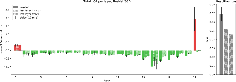
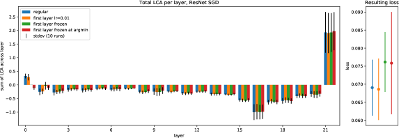
We see an expected pattern for MNIST–FC and MNIST–Lenet (all layers helping; Figure S11), but CIFAR–ResNet with SGD shows a surprising pattern: the first and last layers consistently hurt training (positive total LCA). Over ten runs, the first and last layer in ResNet hurt statistically significantly (p-values $<10^{-4}$ for both), whereas all other layers consistently help (p-values $<10^{-4}$ for all). Blue bars in Figure 4 shows this distinct effect. Such a surprising observation calls for further investigation. The following experiments shed light on why this might be happening.

Figure 4: (left) LCA summed over all of training, for each layer, in CIFAR–ResNet trained with SGD. Bias and batch norm layers are combined into their corresponding kernel layers. Blue represents regular runs. Orange is with the last layer frozen at initialization. Note that the other layers, especially the adjacent few, do not help as much, but the difference in LCA of the last layer is greater than the total differences of the other layers helping less. Green is with the last layer at a 10x smaller learning rate than the rest of the network, showing similar layer LCAs as when the layer is frozen. (right) Resulting train loss and standard deviations for each run configuration. Means and standard deviations are over 10 runs for each experiment configuration.

Freezing the first layer stops it from hurting but causes others to help less.

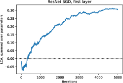
We try various experiments freezing the first layer at its random initialization. Though we can prevent this layer from hurting, the overall performance is not any better because the other layers, especially the neighboring ones, start to help less; see Figure S13 for details. Nonetheless, this can be useful for reducing compute resources during training as you can freeze the first layer without impairing performance.

Freezing the last layer results in significant improvement.

In contrast to the first layer, freezing the last layer at its initialization (Figure 4) improves training performance (and test performance curiously; not shown), with p-values $<0.001$ for both train loss and test loss, over 10 runs! We also observe other layers, especially neighboring ones, not helping as much, but this time the change in the last layer’s LCA more than compensates. Decreasing the learning rate of the last layer by 10x (0.01 as opposed to 0.1 for other layers) results in similar behavior as freezing it. These experiments are consistent with findings in [12] and [8], which demonstrate that you can freeze the last layer in some networks without degrading performance. With LCA, we are now able to provide an explanation for when and why this phenomenon happens. The instability of the last layer at the start of training in [8] can also be measured by LCA, as the LCA of the last layer is typically high in the first few iterations.

Phase shift hypothesis: is the last layer phase-lagged?

While it is interesting to see that decreasing the learning rate by 10x or to zero changes the last layer’s behavior, this on its own does not explain why the layer would end up going backwards. The mini-batch gradient is an unbiased estimator of the whole training set gradient, so on average the dot product of the mini-batch gradient with the training set gradient is positive. Thus we must look beyond noise and learning rate for explanation. We hypothesize that the last layer may be phase lagged with respect to other layers during learning. Intuitively, it may be that while all layers are oscillating during learning, the last layer is always a bit behind. As each parameter swings back and forth across its valley, the shape of its valley is affected by the motion of all other parameters. If one parameter is frozen and all other parameters trained infinitesimally slowly, that parameters valley will tend to flatten out. This means if it had climbed a valley (hurting the loss), it will not be able to fully recover the LCA in the negative direction, as the steep region has been flattened. If the last layer reacts slower than others, its own valley walls may tend to be flattened before it can react.

Figure 5: CIFAR–ResNet SGD with varying momentum for the last layer (and a fixed 0.9 for all other layers). Selected momentum values are derived from linear values of delay $[0,1,2,...,9]$ in a control system, where $\mathrm{momentum}=\mathrm{delay}/(\mathrm{delay}+1)$, and a delay of 9 corresponds to regular runs of 0.9 momentum. (left) LCA per layer (only the second half of the network is shown for better visibility; first half follows a similar trend, but less pronounced). As the last layer helps more, the other layers hurt more because they are relatively more delayed. (right) LCA of the last layer is fairly linear with respect to the delay.

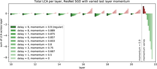
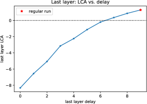
A simple test for this hypothesis is as follows. We note that training with momentum 0.9 corresponds to an information lag of 9 steps (the mean of an exponential series with exponent .9)—each update applied uses information 9 steps old. To give the last layer an advantage, we train it with momentum corresponding to a delay of $n$ for $n\in\{9,8,...,0\}$ while training all other layers as usual. As shown in Figure 5, this works, and the transition from hurting to helping (a lot) is almost linear with respect to delay! As we give the last layer an information freshness advantage, it begins to “steal progress” from other layers, eventually forcing the neighboring layers into positive LCA. These results suggest that it may be profitable to view training as a fundamentally oscillatory process upon which much research in phase-space representations and control system design may come to bear.

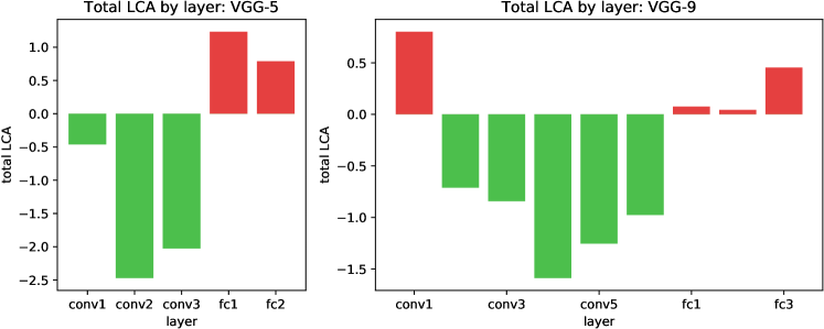
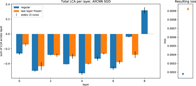
Beyond CIFAR–Resnet, other networks also show intriguingly heterogeneous layer behaviors. As we noted before, in the case of MNIST–FC and MNIST–LeNet trained with SGD, all layers help with varying quantities. An MNIST–ResNet (added specifically to see if the effect we see above is due to the data or the network) shows the last layer hurting as well. We also observe the last layer hurting for CIFAR–AllCNN with SGD (Figure S14) and multiple layers hurting for a couple of VGG-like networks (Figure S12). When using Adam instead of SGD, CIFAR–ResNet has a consistently hurting first layer and an inconsistently hurting last two layers. CIFAR–AllCNN trained with Adam does not have any hurting layers. We note that layers hurting is not a universal phenomenon that will be observed in all networks, but when it does occur, LCA can identify it and suggest potential candidates to freeze. Further, viewing training through the lens of information delay seems valid, which suggests that per-layer optimization adjustments may be beneficial.

5 Learning is synchronized across layers

We learned that layers tend to have their own distinct, consistent behaviors regarding hurting or helping from per-layer LCA summed across all iterations. In this section we further examine the per-layer LCA during training, equivalent to studying individual “loss curves” for each layer, and discover that the exact moments where learning peaks are curiously synchronized across layers. And such synchronization is not driven by only gradients or parameter motion, but both.

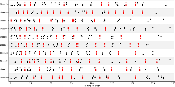
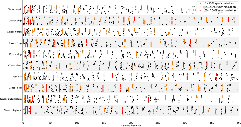
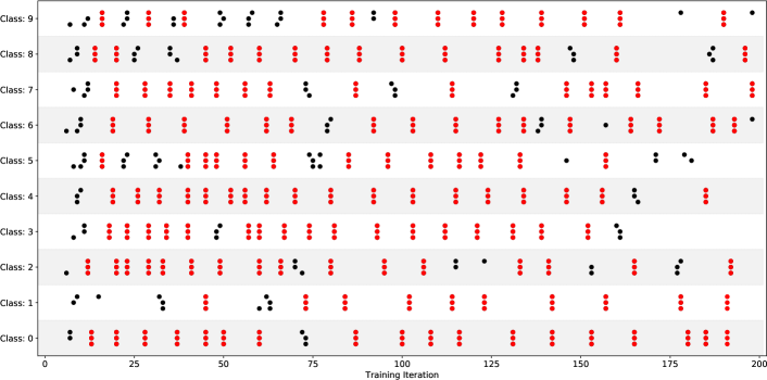
We define “moments of learning” as temporal spikes in an instantaneous LCA curve, local minima where loss decreased more on that iteration than on the iteration before or after, and show the top 20 such moments (highest magnitude of LCA) for each layer in Figure S17. We further decompose this metric by class (10 for both MNIST and CIFAR), where the same moments of learning are identified on per-class, per-layer LCAs, shown in Figure 6. Whenever learning is synchronized across layers (dots that are vertically aligned) they are marked in red. Additional figures on CIFAR–ResNet can be seen in Section S5. The large proportion of red aligned stacks suggests that learning is very locally synchronized across layers.

To gauge statistical significance, we compare the number of synchronized moments in these networks to a simple baseline: the number we would observe if each layer had been randomly shifted to one or two iterations earlier or later. We find that the number synchronized moments is significantly more than that of such a baseline (p-value $<1^{-6}$). See details on this experiment in Section S5. Thus, we conclude that for these networks we’ve measured, learning happens curiously synchronously across layers throughout the network. We might find different behavior in other architectures such as transformer models or recurrent neural nets, which could be of interest for future work.

But what drives such synchronization? Since learning is defined as the product of parameter motion and parameter gradient, we further examine whether one of them is synchronized in the first place. By plotting in the same fashion of identified local peaks, we observe the synchronization pattern in gradients per layer is clearly different from that in LCA, either in terms of the total loss (Figure S18) or per-class loss (Figure S16). Since parameter motion (Figure S19) is the same across all classes, it alone doesn’t drive the per-class LCA. We therefore conclude that the synchronization of learning, demonstrated by synchronized behavior in LCA movement (Figure 6), is strong, and comes from both parameter motion and gradient.

Figure 6: Peak learning iterations by layer by class on MNIST–FC. The same LCA data as in Figure S17 but seperated by class. We plot the top 20 iterations by LCA for each class and each layer, where that iteration represents a local minimum for LCA. The layers are ordered from bottom to top. Points highlighted in red represent iterations where all three layers had peak learning for that particular class. To measure the statistical significance of these vertical line structures in red, we simulate a baseline by shifting each layer in each class randomly by -2, -1, 0, or 1, 2 iteration. We find that the average number of vertical lines is 0.4 in the baseline and 9.4 in the actual network, and this difference is significant with a p-value < 0.001.

6 Conclusion

The Loss Change Allocation method acts as a microscope into the training process, allowing us to examine the inner workings of training with much more fine-grained analysis. When applied to various tasks, networks and training runs, we observe many interesting patterns in neural network training that induce better understanding of training dynamics, and bring about practical model improvements.

6.1 Related work

We note additional connections to existing literature here. The common understanding is that learning in networks is sparse; a subnetwork [6], or a random subspace of parameters [19] is sufficient for optimization and generalization. Our method provides an additional, more accurate, measure of usefulness to characterize per-parameter contribution. A similar work [34] defines per-parameter importance in the same vein but is computed locally with the mini-batch gradient, which overestimates the true per-parameter contribution to the decrease of loss of the whole training set.

Several previous works have increased our understanding of the training process. Alain and Bengio [2] measured and tracked over time the ability to linearly predict the final class output given intermediate layers representations. Raghu et al. [22] found that networks converge to final representations from the bottom up, and class-specific information in networks is formed at various places. Shwartz-Ziv and Tishby [25] visualized the training process through the information plane, where two phases are identified as empirical error minimization of each followed by a slow representation compression. There measurements are developed but none have examine the process each individual parameter undergoes.

Methods like saliency maps [27], DeepVis [33], and others allow interpretation of representations or loss surfaces. But these works only approach the end result of the model, not the training process in progress. LCA can be seen as a new tool that specializes on the microscopic level of details, and such inspection follows through the whole training process to reveal interesting facts about learning. Some of our findings resonate with and complement other work. For example, in [35] it is also observed that layers have heterogeneous characteristics; in that work layers are denoted as either “robust” or “critical”, and robust layers can even be reset to their initial value with no negative consequence.

6.2 Future work

There are many potential directions to expand this work. Due to the expensive computation and the amount of analyses, we have only tested vision classification tasks on relatively small datasets so far. In the future we would like to run this on larger datasets and tasks beyond supervised learning, since the LCA method directly works on any parameterized model. An avenue to get past the expensive computation is to analyze how well this method can be approximated with gradients of loss of a subset of the training set. We are interested to see if the observations we made hold beyond the vision task and the range of hyperparameters used.

Since per-weight LCA can be seen as a measurement of weight importance, an simple extension is to perform weight pruning with it, as done in [6, 36] (where weight’s final value is used as an importance measure). Further, if there are strong correlations between underperforming hyperparameters and patterns of LCA, this may help in architecture search or identifying better hyperparameters.

We are also already able to identify which layers or parameters overfit by comparing their LCA on the training set and LCA on the validation or test set, which motions towards future work on targeted regularization. Finally, the observations about the noise, oscillations, and phase delays can potentially lead to improved optimization methods.

 

Supplementary Information for:
LCA: Loss Change Allocation for
Neural Network Training

 

S1 Supplementary results: Method

Table S1: Summary of errors of the LCA method with the Runge-Kutta method (RK4) used in our analyses, as well as the first order Taylor approximation (FO) for comparison. “Total error” is the percent error of total change in loss based on LCA vs. actual total change in loss over all iterations, where negative means that LCA gave a lower final loss. “Average iteration error” is the absolute error in one iteration, averaged over all iterations. Positive and negative errors at individual iterations could hypothetically cancel out somewhat when summed over all of training, though this is clearly not the case for first order, as it consistently and severely overestimates how much the loss decreases. This conforms with observations of the loss landscape being biased toward positive curvature. Reported numbers are averaged over 3 runs per configuration.

	Total error, RK4	Total error, FO	Average iteration error, RK4	Average iteration error, FO
MNIST-FC, SGD mom=0	-0.27%	-4249.64%	6.11E-05	0.11400
MNIST-FC, SGD	1.08E-03%	-171.10%	2.94E-06	0.00459
MNIST-FC, Adam	3.64E-03%	-75.31%	2.31E-06	0.00199
MNIST-LeNet, SGD	1.87E-02%	-274.84%	3.45E-06	0.00838
MNIST-LeNet, Adam	0.0262%	-498.67%	2.30E-06	0.01499
CIFAR-ResNet, SGD	0.0345%	-1189.71%	1.37E-05	0.01018
CIFAR-ResNet, Adam	0.0537%	-923.88%	1.07E-05	0.00793
CIFAR-AllCNN, SGD	0.1374%	-1371.69%	4.51E-06	0.00662
CIFAR-AllCNN, Adam	0.0745%	-972.61%	2.77E-06	0.00482

S2 Supplementary results: Direct visualization

Examples of additional direct visualization methods shown in Figure S1 and Figure S2. Section S6 shows other possible visualizations with aggregations over neurons or channels.

Figure S1: First layer of MNIST–LeNet with Adam. Rather than displaying all parameters in one iteration, we can sum up parameters within each output channel of this layer. The other axis can now be used to display all iterations.

Figure S2: Cumulative LCA for individual parameters in the first layer of MNIST–LeNet with Adam. Left: the 50 (out of 500) most helpful parameters (most negative LCA). Right: a random set of 50 parameters. You can see that the typical parameter’s cumulative LCA drops quickly near the beginning and then continues to wiggle slightly after flattening out. Some parameters are mostly flat after the initial drop, but others continue learning slightly until the end.

S3 Supplementary results: Learning is very noisy

We provide plots from Section 3 for all networks here in Figure S3, Figure S4, Figure S5, and Figure S6.

Plots of oscillation shown in Figure S7 and Figure S8 for ResNet, and additional oscillation measurements in Table S2 for all networks.

Adjusting hyperparameters has some effect on the percent of parameters helping, shown in Figure S9. However, the percent helped remains within a small range, especially when ignoring points of significantly worse test performance (rightmost points for momentum and mini-batch size).

Figure S3: MNIST–FC. Top: SGD with no momentum, middle: SGD with momentum = 0.9, bottom: Adam. Figures display the same measurements as in Figure 3, except the histogram of all LCA values now shows all values rather than ignoring the 1% tails.

Figure S4: MNIST–LeNet. Top: SGD, bottom: Adam

Figure S5: CIFAR–ResNet. Top: SGD, bottom: Adam

Figure S6: CIFAR–AllCNN. Top: SGD, bottom: Adam

Figure S7: Oscillations for CIFAR–ResNet with SGD. Left: number of times the weight movement oscillates. Right: number of times the gradient crosses zero from one iteration to the next. Values shown are number of iterations out of 5000, averaged over all parameters within a layer. The averages over the entire network are 741.9 for weight turns and 525.8 for gradients crossing zero. Note that the first and last layers oscillate more than their neighboring layers, which is interesting given that those layers hurt (Section 4), but this is only a correlation as oscillations do not explain why something would bias towards helping or hurting.

Figure S8: Oscillations of two individual parameters of the last kernel layer in CIFAR–ResNet with SGD. We look at iterations 50-200 (first 50 skipped due to large fluctuations), and display the parameter that hurt the most (top) and the parameter that helped the most (bottom) in these given iterations (net LCA of +3.41e-3 and -3.03e-3, respectively). Here, we visualize the weight movements (orange) along with their gradient values (blue) of the loss of the whole training set w.r.t. that parameter. Note that the trajectory of gradients and weights have similar shapes, indicating that these parameters are oscillating back and forth over a parabolic local minima that is shifting slightly (as the other parameters of the network are changing). During one back-and-forth cycle, the parameter will help, then hurt once the gradient crosses zero but momentum causes the weight to keep moving in the same direction, then help as the weight movement switches direction, and then hurt again when the gradient crosses zero again. This swinging LCA is depicted in the green and red bars. Because of these oscillations, the parameters end up helping approximately half the time and hurting the other half. While this behavior does not account for all the noise in other parameters and other iterations, it is commonly present.

Table S2: Two metrics on oscillation: for each parameter, we look at the weight movement and count how often it switches direction (derivative of weight value changes sign) from one iteration to the next. We also look at the gradient for that parameter, and count how often it crosses zero (changes sign) from one iteration to the next. We convert both these into average frequencies over the training process, and then average those over all parameters in the network. These two measures are related – if a parameter oscillates around a local minima, its gradient would cross zero every time the weight changes direction – but due to noise, they do not have to correspond 1:1.

Network	Number of iterations per weight movement direction change	Number of iterations every time gradient crosses zero
MNIST–FC, SGD mom=0	3.49	3.48
MNIST–FC, SGD	13.57	11.68
MNIST–FC, Adam	12.68	12.71
MNIST–LeNet, SGD	10.29	9.37
MNIST–LeNet, Adam	16.86	15.37
CIFAR–ResNet, SGD	6.74	9.51
CIFAR–ResNet, Adam	6.76	9.81
CIFAR–AllCNN, SGD	7.06	11.18
CIFAR–AllCNN, Adam	6.76	10.37

Figure S9: Effects of different hyperparameter values on the percent of parameters helped per iteration, for CIFAR–ResNet with SGD. Left: learning rate, middle: momentum, right: mini-batch size. While there is some change in the percent helped, it does not go below 50.3% or above 51.6% within hyperparmeter ranges that still allow the network to learn. This excludes the configuration of momentum = 0.99 with 53.5% helped, where train and test performance have both degraded, and the number of parameters with zero LCA has actually significantly increased (resulting in 27.6% helped, 48.5% zero, 23.9% hurt). Also, as we increase the mini-batch size to 5000 (1/10th of the training data), the percent helped reaches 56.2%, but this is not practical as the test performance has become significantly worse.

Figure S10: A depiction of how LCA distributions are significantly more heavy-tailed than a Gaussian distribution. A kurtosis test on the actual distribution against a Gaussian gives excess kurtosis of 10420 and a p-value of effectively 0. The actual distribution has kurtosis of 2141, averaged across iteration intervals

S4 Supplementary results: Some layers hurt overall

Additional plots: Figure S11 comparing 3 different networks, Figure S12 demonstrating the phenomenom of layers hurting for additional network architectures, Figure S13 for experiments concerning the first layer of CIFAR–ResNet, SGD, and Figure S14 concerning the last layer of CIFAR–AllCNN, SGD.

Figure S11: LCA summed over all of training, across each layer. Bias and batch norm layers are combined into their corresponding kernel layers. Left: MNIST–FC, middle: MNIST–LeNet, right: CIFAR–ResNet, all using SGD. While there is variation in the FC and LeNet layers (magnitudes are somewhat correlated to the size of the layer), they all are helping with negative LCA. On the other hand, the first and last layers of the ResNet strangely have positive LCA.

Figure S12: LCA of layers for two VGG-like models to further demonstrate that layers hurting is not a special one-off observation. It is also interesting to note that multiple layers hurt in these networks. Left: VGG-5 has 3 conv2D layers with 3x3 filters and {64, 128, 256} output channels, each followed by max pooling of stride 2, and then two fully connected layers with {512, 10} output units. Right: VGG-9 is the same as the VGG-11 used in [26] except with the last 2 conv2D layers removed, half the output channels in the remaining conv2D layers, and {512, 512, 10} output channels on the fully connected layers.

Figure S13: Left: LCA summed over all of training and across each layer of CIFAR–ResNet on SGD. Bias and batch norm layers are combined into their corresponding kernel layers. Blue represents a normal run configuration, and other colors show various experiments on the first layer. When the first layer uses a 10x smaller learning rate than the other layers (orange), per-layer LCA does not change much. While the “first layer frozen” runs (green) no longer hurt in the first layer (since the layer parameters are frozen from the beginning), the other layers, especially the next two, do not help as much. A similar effect is seen when we freeze the first layer at its LCA argmin (red); while we force the first layer to have negative LCA, the others have slightly more positive LCA, thus cancelling out any improvements. Middle: resulting train loss for each run configuration and standard deviations. Right: a typical cumulative trajectory of the first layer’s learning, which helps in the first few hundred iterations and then increasingly hurts. The “freeze first layer at argmin” lets the layer help first before freezing it, but that still doesn’t improve performance.

Figure S14: LCA for AllCNN layers. Last layer hurts in a regular run (blue), but freezing the last layer at initialization (orange) results in a worse overall loss (shown on the right).

S5 Supplementary results: Learning is synchronized across layers

Figure S15: Peak learning iterations by layer by class on CIFAR–ResNet. We consider the first 400 training iterations, by which point the network achieves a test accuracy of 65%. We plot the top 20 iterations by LCA for each class and each layer, where that iteration represents a local minimum for LCA. The layers are ordered from bottom to top. Points highlighted in orange represent iterations where 25% to 50% of the kernel layers (6 to 10) had peak learning for that particular class, and there are 16.6 lines on average. Points highlighted in red represent iterations where at least 50% of the kernel layers (11 or more) had peak learning for that particular class, and there are 5.8 lines on average.

Figure S16: Peak effective gradient iterations by layer by class on MNIST–FC.

Figure S17: Peak learning iterations by layer on MNIST–FC. Eeah row represents a layer in the 3-layer FC network, orderred from bottom to top. Dots indicate top 20 moments of learning. and marked in red whenever synchronized across all layers. In this example 12 out of 20 moments are synchronized. The number of synchronized learning iterations is significantly more than chance, with a p-value of <0.001.

Figure S18: Peak effective gradients iterations by layer on MNIST–FC.

Figure S19: Peak weight movement iterations by class on MNIST–FC.

S6 Supplementary results: Additional observations

S6.1 Trajectory of parameters and temporal correlations

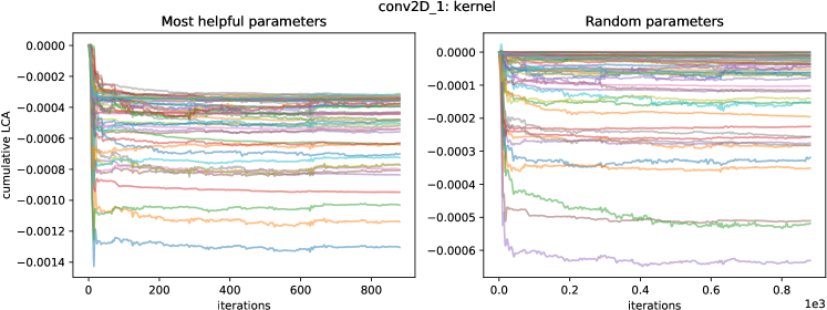
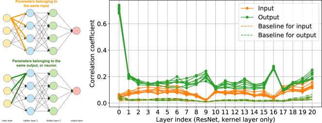
Our method allows for each individual parameter to have its own “loss curve”, or, cumulative LCA, as seen in Figure S2. Interestingly, parameters going into the same neuron tend to have similar loss curves, meaning that they learn together. This can also be seen in the animations in Figure 2. We prove this concept with a correlation metric and statistical test. We conduct experiments for every layer in a network (focusing on kernel parameters, or weights, and ignoring bias and batch normalization parameters), calculate correlation coefficients of pairs of parameters, and apply Kolmogorov-Smirnov test to measurements for statistical significance. We find significantly stronger correlations between parameters of the same inputs or outputs than a random baseline, as depicted in Figure S20.

Figure S20: Correlation of weights within inputs and outputs, for every kernel layer of CIFAR-ResNet. (Left) Schematic indicating how weights belonging to the same input/output is like. (Right) Measured correlations for each layer. Multiple lines indicate multiple runs. For each layer, for each input/output, take all the weights going belonging to it, calculate pairwise correlation coefficients and the average of them. Then average through all nodes of that layer. Baseline for it is a constructed "fake node" with the same number of weights (or the most that exist), where no pair is from the same input or output.

S6.2 Class specialization in neurons

It is generally known that earlier layers in a neuron network learn more general concepts than later layers. This is akin to measuring the degree to which individual neurons specialize in learning specific classes. We can now show precisely how specialized neurons are and how this pattern evolves as we go deeper in the network.

Figure S21: (Left) MNIST–FC. (Right) CIFAR–ResNet. Fraction of neurons that concentrate on learning 1, 2, or 3 classes. For each neuron in each layer, we compute the ratio between amount helped for the top 1, 2, or 3 class(es) and the total amount helped for all positively benefited classes. We then find the fraction of neurons in each layer where the top 1, 2, or 3 class(es) contributed more than 80% of total learning.

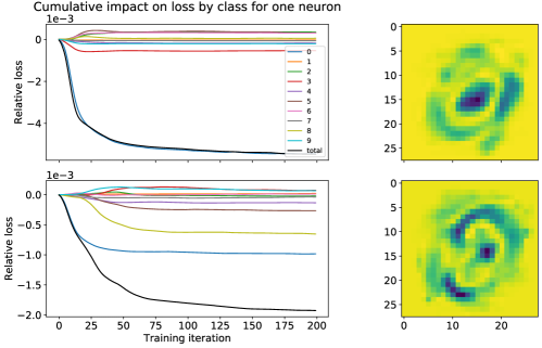
We can also identify neurons that specialize in certain classes and visualize their behavior. For example, we look at two neurons in Figure S22 that concentrated on learning one and two classes, respectively. A saliency map using amount helped for each neuron gives us some insight into what that neuron is learning. A similar plot using just the weight values do not hold a clear pattern.

Figure S22: (Top) An example of a first layer neuron that concentrated on learning the 0 class. (Bottom) An example of a first layer neuron that concentrated on learning the 0 and 8 classes. (Left) Cumulative amount helped by class. (Right) Plot of the 784 parameters within this neuron reshaped as a 2D image, colored by the LCA for each parameter.

S7 Additional details on model architectures and training hyperparameters

All layers in network are followed by ReLu nonlinearity, and weights are initialized according to the He-normal distribution [10]. Exact implementation details can be found in our public codebase at https://github.com/uber-research/loss-change-allocation.

MNIST–FC

We use a three-layer fully connected network, of sizes 100, 50, 10. For simplicity, no batch normalization or dropout was used.

MNIST–LeNet

First conv layer is 5x5, 20 filters, followed by a 2x2 max pool of stride 2. Second conv layer is also 5x5, 40 filters, followed by a 2x2 max pool of stride 2 and dropout of 0.25. The result is flattened and fed through two fully connected networks with output sizes 400 and 10.

CIFAR–AllCNN

AllCNN is the same as described in [29], with 9 convolutional layers followed by global average pooling. Batch normalization [13] and dropout [11] are used. The table below lists the size of layers and where batch normalization and dropout are added.

3x3 conv, 96	followed by batch normalization
3x3 conv, 96	followed by batch normalization
3x3 conv, 96	Stride 2, followed by 0.5 dropout
3x3 conv, 192	followed by batch normalization
3x3 conv, 192	followed by batch normalization
3x3 conv, 192	Stride 2, followed by 0.5 dropout
3x3 conv, 192	followed by batch normalization
1x1 conv, 192	followed by batch normalization
1x1 conv, 10
Global average pooling

CIFAR–ResNet20

Each residual block consists of two 3x3 conv layers with the specified number of filters. Shortcuts are added directly if the number of filters is the same between blocks, otherwise the dimension change is done by a 1x1 conv with stride 2.

3x3 conv, 16
[Residual block of 16] x 3
[Residual block of 32] x 3
[Residual block of 64] x 3
Global average pooling
Fully connected, 10 outputs

Hyperparameter search

We adjusted learning rate based on validation accuracy. The range we tried is an approximate log scale [1, 2, 5] times different powers of ten from 0.0005 to 1. Early stopping iteration was selected by when validation accuracy has flattened and train is mostly complete. For momentum, batch size, and dropout rates, we used reasonable and common values. We did not tune these (unless noted in special experiments) as they worked well and the exact values were not important. We used the given training/validation/testing split in the MNIST and CIFAR datasets.

For the LCA method, we also tried trapezoid rule, midpoint rule, and Boole’s rule, and found that the Runge-Kutta method worked best given the same amount of computation.

Learning rates used

The following learning rates are used in default experiments (SGD uses 0.9 momentum if not otherwise stated):

	SGD	Adam
MNIST–FC, no momentum	0.5	N/A
MNIST–FC	0.05	0.002
MNIST–LeNet	0.02	0.002
CIFAR–ResNet	0.1	0.005
CIFAR–AllCNN	0.1	0.001

S8 Computational considerations

Consider the two terms of Equation 3. The second term, $\theta_{t+1}^{(i)}-\theta_{t}^{(i)}$, depends on the path taken by the optimizer through $\theta$ space, which in turn depends only on the gradients of mini-batches from the training set. This term is readily available during typical training scenarios without requiring extra computation. In contrast, the first term, $\nabla_{\theta}L(\theta_{t})$, is computed over the entire training set and is not available in typical training. It must be computed separately, and because it requires evaluation of the entire training set, this computation is expensive (if the entire training set is $N$ times larger than your mini-batch, each iteration would take approximately $N$ times as long). Evaluating the loss and gradients over the entire training set at every training iteration may seem intractably slow, but in fact for smaller models and datasets, using modern GPUs we can compute this gradient in a reasonable amount of time, for example, 0.2 seconds per gradient calculation for a simple fully connected (FC) network on the MNIST dataset or 9 seconds for the ResNet-20 [9] model on the CIFAR-10 dataset. These times are quoted using a single GPU, but to speed calculations we distributed gradient calculations across four GPUs (we used NVIDIA GeForce GTX 1080 Ti). Thus, although the approach is slow, it is tractable for small to medium models.

Model	Number of trainable params	Training time and iterations used	Time per iteration of gradient calculations on one GPU	Storage space per iteration
MNIST–FC	84,060	4 min,	0.4 s	300 kb
		880 iterations
MNIST–LeNet	808,970	11-12 min	2.4 s	3.5 mb
		880 iterations
CIFAR–ResNet20	273,066	120-125 min,	18-20 s	1.2 mb
		5000 iterations
CIFAR–AllCNN	1,371,658	270-280 min,	36-42 s	6 mb
		5000 iterations

References

- Achille et al. [2017] Alessandro Achille, Matteo Rovere, and Stefano Soatto. Critical learning periods in deep neural networks. CoRR, abs/1711.08856, 2017. URL http://arxiv.org/abs/1711.08856.
- Alain and Bengio [2016] G. Alain and Y. Bengio. Understanding intermediate layers using linear classifier probes. ArXiv e-prints, October 2016.
- Bottou et al. [2018] Léon Bottou, Frank E Curtis, and Jorge Nocedal. Optimization methods for large-scale machine learning. Siam Review, 60(2):223–311, 2018.
- Choromanska et al. [2015] Anna Choromanska, Mikael Henaff, Michael Mathieu, Gérard Ben Arous, and Yann LeCun. The loss surfaces of multilayer networks. In Artificial Intelligence and Statistics, pages 192–204, 2015.
- Dauphin et al. [2014] Yann N Dauphin, Razvan Pascanu, Caglar Gulcehre, Kyunghyun Cho, Surya Ganguli, and Yoshua Bengio. Identifying and attacking the saddle point problem in high-dimensional non-convex optimization. In Advances in neural information processing systems, pages 2933–2941, 2014.
- Frankle and Carbin [2019] Jonathan Frankle and Michael Carbin. The lottery ticket hypothesis: Finding sparse, trainable neural networks. In International Conference on Learning Representations (ICLR), volume abs/1803.03635, 2019. URL http://arxiv.org/abs/1803.03635.
- Goodfellow et al. [2014] Ian J Goodfellow, Oriol Vinyals, and Andrew M Saxe. Qualitatively characterizing neural network optimization problems. arXiv preprint arXiv:1412.6544, 2014.
- Gotmare et al. [2019] Akhilesh Gotmare, Nitish Shirish Keskar, Caiming Xiong, and Richard Socher. A closer look at deep learning heuristics: Learning rate restarts, warmup and distillation. In International Conference on Learning Representations, 2019. URL https://openreview.net/forum?id=r14EOsCqKX.
- He et al. [2015a] Kaiming He, Xiangyu Zhang, Shaoqing Ren, and Jian Sun. Deep residual learning for image recognition. CoRR, abs/1512.03385, 2015a. URL http://arxiv.org/abs/1512.03385.
- He et al. [2015b] Kaiming He, Xiangyu Zhang, Shaoqing Ren, and Jian Sun. Delving deep into rectifiers: Surpassing human-level performance on imagenet classification. In Proceedings of the IEEE international conference on computer vision, pages 1026–1034, 2015b.
- Hinton et al. [2012] Geoffrey E Hinton, Nitish Srivastava, Alex Krizhevsky, Ilya Sutskever, and Ruslan R Salakhutdinov. Improving neural networks by preventing co-adaptation of feature detectors. arXiv preprint arXiv:1207.0580, 2012.
- Hoffer et al. [2018] Elad Hoffer, Itay Hubara, and Daniel Soudry. Fix your classifier: the marginal value of training the last weight layer. CoRR, abs/1801.04540, 2018. URL http://arxiv.org/abs/1801.04540.
- Ioffe and Szegedy [2015] Sergey Ioffe and Christian Szegedy. Batch normalization: Accelerating deep network training by reducing internal covariate shift. CoRR, abs/1502.03167, 2015. URL http://arxiv.org/abs/1502.03167.
- Jastrzębski et al. [2019] Stanisław Jastrzębski, Zachary Kenton, Nicolas Ballas, Asja Fischer, Yoshua Bengio, and Amos Storkey. On the Relation Between the Sharpest Directions of DNN Loss and the SGD Step Length. In International Conference on Learning Representations (ICLR), page arXiv:1807.05031, Jul 2019.
- Keskar et al. [2016] Nitish Shirish Keskar, Dheevatsa Mudigere, Jorge Nocedal, Mikhail Smelyanskiy, and Ping Tak Peter Tang. On large-batch training for deep learning: Generalization gap and sharp minima. arXiv preprint arXiv:1609.04836, 2016.
- Kirkpatrick et al. [2017] James Kirkpatrick, Razvan Pascanu, Neil Rabinowitz, Joel Veness, Guillaume Desjardins, Andrei A. Rusu, Kieran Milan, John Quan, Tiago Ramalho, Agnieszka Grabska-Barwinska, Demis Hassabis, Claudia Clopath, Dharshan Kumaran, and Raia Hadsell. Overcoming catastrophic forgetting in neural networks. Proceedings of the National Academy of Sciences, 114(13):3521–3526, 2017. doi: 10.1073/pnas.1611835114. URL http://www.pnas.org/content/114/13/3521.abstract.
- Kutta [1901] Wilhelm Kutta. Beitrag zur näherungweisen integration totaler differentialgleichungen. 1901.
- LeCun et al. [1998] Yann LeCun, Léon Bottou, Yoshua Bengio, and Patrick Haffner. Gradient-based learning applied to document recognition. Proceedings of the IEEE, 86(11):2278–2324, 1998.
- Li et al. [2018] Chunyuan Li, Heerad Farkhoor, Rosanne Liu, and Jason Yosinski. Measuring the Intrinsic Dimension of Objective Landscapes. In International Conference on Learning Representations, April 2018.
- Li et al. [2018] Hao Li, Zheng Xu, Gavin Taylor, Christoph Studer, and Tom Goldstein. Visualizing the loss landscape of neural nets. In Advances in Neural Information Processing Systems, pages 6389–6399, 2018.
- Nguyen and Hein [2017] Quynh Nguyen and Matthias Hein. The loss surface of deep and wide neural networks. In Proceedings of the 34th International Conference on Machine Learning-Volume 70, pages 2603–2612. JMLR. org, 2017.
- Raghu et al. [2017] M. Raghu, J. Gilmer, J. Yosinski, and J. Sohl-Dickstein. Svcca: Singular vector canonical correlation analysis for deep learning dynamics and interpretability. ArXiv e-prints, June 2017.
- Runge [1895] Carl Runge. Über die numerische auflösung von differentialgleichungen. Mathematische Annalen, 46(2):167–178, 1895.
- Safran and Shamir [2016] Itay Safran and Ohad Shamir. On the quality of the initial basin in overspecified neural networks. In International Conference on Machine Learning, pages 774–782, 2016.
- Shwartz-Ziv and Tishby [2017] Ravid Shwartz-Ziv and Naftali Tishby. Opening the black box of deep neural networks via information. CoRR, abs/1703.00810, 2017. URL http://arxiv.org/abs/1703.00810.
- Simonyan and Zisserman [2014] Karen Simonyan and Andrew Zisserman. Very deep convolutional networks for large-scale image recognition. CoRR, abs/1409.1556, 2014. URL http://arxiv.org/abs/1409.1556.
- Simonyan et al. [2013] Karen Simonyan, Andrea Vedaldi, and Andrew Zisserman. Deep inside convolutional networks: Visualising image classification models and saliency maps. arXiv preprint arXiv:1312.6034, presented at ICLR Workshop 2014, 2013.
- Soudry and Carmon [2016] Daniel Soudry and Yair Carmon. No bad local minima: Data independent training error guarantees for multilayer neural networks. arXiv preprint arXiv:1605.08361, 2016.
- Springenberg et al. [2014] Jost Tobias Springenberg, Alexey Dosovitskiy, Thomas Brox, and Martin A. Riedmiller. Striving for simplicity: The all convolutional net. CoRR, abs/1412.6806, 2014. URL http://arxiv.org/abs/1412.6806.
- Sutskever et al. [2013] Ilya Sutskever, James Martens, George Dahl, and Geoffrey Hinton. On the importance of initialization and momentum in deep learning. In International conference on machine learning, pages 1139–1147, 2013.
- Weisstein [2003] Eric W Weisstein. Simpson’s rule. 2003.
- Xing et al. [2018] Chen Xing, Devansh Arpit, Christos Tsirigotis, and Yoshua Bengio. A walk with sgd. 2018.
- Yosinski et al. [2015] J. Yosinski, J. Clune, A. Nguyen, T. Fuchs, and H. Lipson. Understanding Neural Networks Through Deep Visualization. ArXiv e-prints, June 2015.
- Zenke et al. [2017] Friedemann Zenke, Ben Poole, and Surya Ganguli. Improved multitask learning through synaptic intelligence. CoRR, abs/1703.04200, 2017. URL http://arxiv.org/abs/1703.04200.
- Zhang et al. [2019] Chiyuan Zhang, Samy Bengio, and Yoram Singer. Are all layers created equal? arXiv preprint arXiv:1902.01996, 2019.
- Zhou et al. [2019] Hattie Zhou, Janice Lan, Rosanne Liu, and Jason Yosinski. Deconstructing lottery tickets: Zeros, signs, and the supermask. arXiv preprint arXiv:1905.01067, 2019.