An intricate quantum statistical effect
and the foundation of quantum mechanics

Abstract

An intricate quantum statistical effect guides us to a deterministic, non-causal quantum universe with given fixed initial and final state density matrix. A concept is developed on how and where something like macroscopic physics can emerge.

The concept does not allow to incorporate philosophically indispensable free will decisions. If the quantum world and its conjugate evolve independently one can replace both fixed final states by a matching common one. This allows for external manipulations done in the quantum world and its conjugate which do not otherwise alter the basic structure.

In a big bang / big crunch universe the expanding part can be attributed to the quantum world and the contracting part to the conjugate one. The obtained bi-linear picture has a number of beautiful and exciting consequences.

Introduction

The interrelation of classical and quantum physics is revisited. It is in my opinion treated in some way too timidly and I advocated a new approach yielding an appealing concept Bopp:2018kiw ; Bopp:2016nxn ; bopp2019bi . My aim here is to develop the basic argument considerably more thoroughly than previously done.

It is not meant as an exercise in finely nuanced words. Nevertheless two definitions are necessary:

QUANTUM DYNAMICS
$=$

quantum mechanics
without measurements
$\in$

relativistic quantum field theory

MACROSCOPIC DYNAMICS
$=$

classical mechanics

$+$ classical electrodynamics

$+$ most of statistical mechanics

$+$ parts of general relativity

The first definition was coined by Sakurai sakurai2014modern . Quantum dynamics means quantum mechanics (QM) without measurements. Meant are the von Neumann projection operators, i.e. the jumps. Decoherence joos2013decoherence is part of quantum dynamics. Sakurai made the point that all the spectacular achievements of QM actually lie in the domain of quantum dynamics. Underlying quantum dynamics is, of course, relativistic quantum field theory. For the considered questions they are identical. The second definition is almost trivial. It is given in the above right box.

Both world views differ in a central way. In macroscopic dynamics there is a unique path way. Ensembles are often specified in a limited way. But it just reflects ignorance. On a fundamental level there is at each point in time one true configuration.

This is of course different in quantum dynamics. Here many distinct path ways can coexist. What is meant with distinct? Topologically Feynman paths are distinct if they belong to different homotopy classes. Paths going though the upper and the lower gap of a two slit experiment are distinct. Essentially it is assumed that Feynman paths in a homotopy class can be integrated out to an effective ,,real” path way. For a more careful consideration how real paths arise I refer to wharton2015towards .

The hard conclusion is: Both world views are incompatible! It was recognized early on einstein1935can ; bohr1935can . Historically the basic premise seems to have been that something was missing in the young QM and that one had somehow to repair it by a suitable amendment. An example of such an attempt is de Broglie - Bohm guiding field theory de1927mecanique ; bohm1952suggested ; durr2009bohmian . Almost a century has passed and a lot of serious work was done investigating all aspects feynman1948space ; Kiefer2008siegen ; wheeler2014quantum ; e21050447 ; Hooft:2016Cellular ; mermin1998quantum ; bopp1966elementarvorgaenge ; sussmann1952spontane ; Davidson2017 ; Davidson:2017ilu ; zeh2001physical ; zurek2003decoherence ; hossenfelder2019rethinking . There are various proposed interpretations to solve the problem or at least make the ”incompatibility” acceptable. However, it is fair to say that this was not fully successful. No interpretation is generally accepted.

My basic concept to avoid the incompatibility will be not to change quantum dynamics but macroscopic dynamics. In literature there are various observations requiring such changes. As outlined in a recent review of Wharton and Argaman wharton2019bell whatever one does on the quantum theoretical side aspects of the macroscopic dynamics have to change as they disagree with Bell type experiments bell1964einstein . I will take a more radical position to question everything we think to know of macroscopic dynamics. It will be taken as independent theory. In only holds approximately and only in our epoch in the universe.

On the other hand quantum dynamics will be considered an exact theory of the whole universe. It is the only theory confirmed on a 16 digit level (for QED anomalous moments hernandez1990review ) and it is quite reasonably to be taken as a safe base. The task will be then how something like causal macroscopic dynamics comes out of the unamended non-causal quantum dynamics.

In the next section the basic argumentation will be presented. It will contain no ad hoc assumptions. A straight forward consideration then, in section 3, will lead to a completely deterministic concept. To allow for ,,free will” a suitable modification with a bi-directional universe will be introduced in section 4. A discussion of consequences follows.

1 Measurements

Figure 1: Stern-Gerlach arrangement

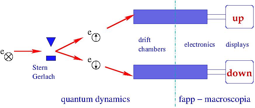
The traditional bridge between quantum dynamics and the macroscopic world are measurements. To proceed consider a simple generic arrangement shown in figure 1. An electron with an ,,in the black board” spin get split in an inhomogeneous magnetic field. Its ,,up” resp. ,,down” component enters a drift chamber where lots of photons of various frequencies are produced and a few electrons are kicked of their atoms and collected. Suitable charge coupled electronics flashes ,,up” resp. ,,down” on displays.

Figure 2: Stern-Gerlach measurement

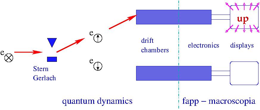
Empirically also the here just effective macroscopic dynamics requires no co-exiting pathways. So there has to be a decision leading e.g. to figure 2.

What does this decision mean? Many authors see a violation of locality. In the framework of a simple relativistic theory this is - taken verbatim - wrong.

Consider the needed part of Bohm’s version of the Einstein-Rosen-Podolsky experiment bohm1951quantum . A spin-less ion emits two electrons to form a spin-less ground state. Obviously both electrons have to have opposite spins. If Bob measures the spin to be in ,,up” direction the electron coming to Alice will have a spin in ,,down” direction and Alice will measure ,,down” and vice versus. If Bob measures the spin sidewise independent of his result the electron coming to Alice will not know whether Alice will measure ,,up” or ,,down”. In this way Bob’s decision changes the nature of the electron coming to Alice.

It is well known Bob is a relatively shy one. So he will be at least twice as far from the exited atom as Alice. In some Lorentz system Alice‘s measurement will be in Bob’s past and with his measurement he influences a property of an electron in his past. That means backward causation and what is violated is causality leifer2017time ; aharonov2015can . It is not a trivial distinction:

$$\mathrm{backward\,causality}\cup\mathrm{forward\,causality}\Rightarrow\mathrm{non\,locality}$$

but

$$\mathrm{non\,locality}\not\Rightarrow\mathrm{backward\,light\,cone\,causality}\,.$$

To give up causality is very serious and not widely accepted. A customary defense is to deny ontological reality of the electron wave going to Alice. It opens up intensively discussed interpretations. Some physicists find it not appealing. They want to know what is really going on and not just have a law to predict outcomes. Nevertheless non-causality is hard to accept and for the considered situations this Copenhagen interpretation has to be considered as most reasonable choice. It was advocated by most physicists we admire.

However there are quantum statistical effects Bopp:2018kiw ; Bopp:2016nxn ; bopp2001ulm ; bopp2019bi which in my opinion change the conclusion. This is a central point which I contemplated for many years. They are unfortunately rarely discussed. Field theoretical results do not involve von Neumann measurement and even famous people tend to claim ignorance to questions involving jumps. In the quantum optics community one encounters a feeling that problems with Schrödinger‘s equation are difficult enough and that it is reasonable to postpone questions involving second quantization.

So it will not be easy to be convincing. There are several versions. A quantum statistical effect in high energy heavy ion scattering considering Bose Einstein enhancement might be the best hope as it is closest to my background Abreu:2007kv . It is one of what Glauber called ,,known crazy” effects glauberISMD .

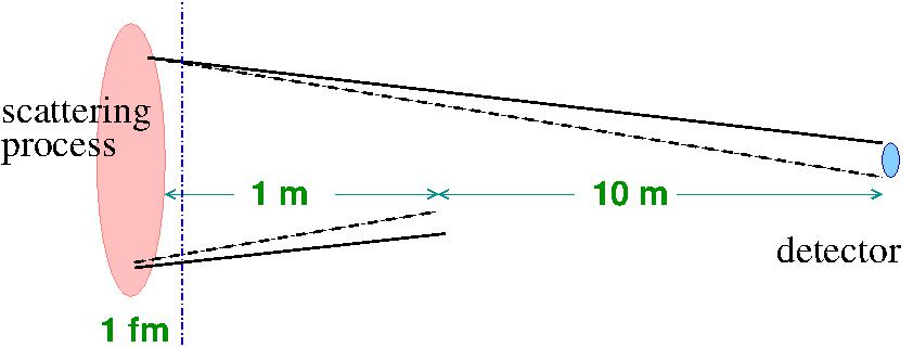
For non experts the description of high energy heavy ion scattering usually involves a somewhat simple pictures mixing coordinate and momentum space. It assumes - not really knowing the actually needed $\pi N$ Hamiltonian - that both fast incoming more or less round nuclei are in the central system Lorentz contracted to pancake shaped objects. The actual scattering is then assumed to take place when the pancakes overlap in the narrow region shown as red in the figure 3.

Lots of particles are produced including two say $\pi^{+}$’s with the momenta $Q_{1}$ and $Q_{2}$. I denote the amplitude as $A(1,2)$. As $\pi^{+}$’s are bosons also the crossed contribution shown as dashed line in the figure has to be included and the probability of such a process is:

emission probability $=$

$${=\frac{1}{2}|A(1,2)+A(2,1)|^{2}=\,\begin{cases}2\cdot|A(1,2)|^{2}&\mathrm{for}\,Q_{1}=Q_{2}\\ 1\cdot|A(1,2)|^{2}&\mathrm{for}\,Q_{1}\neq Q_{2}\,\mathrm{but}\,Q_{1}\sim Q_{2}\end{cases}}$$ (1)

Figure 3: Two emitted ${\pi^{+}}^{\prime}s$

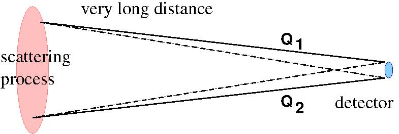
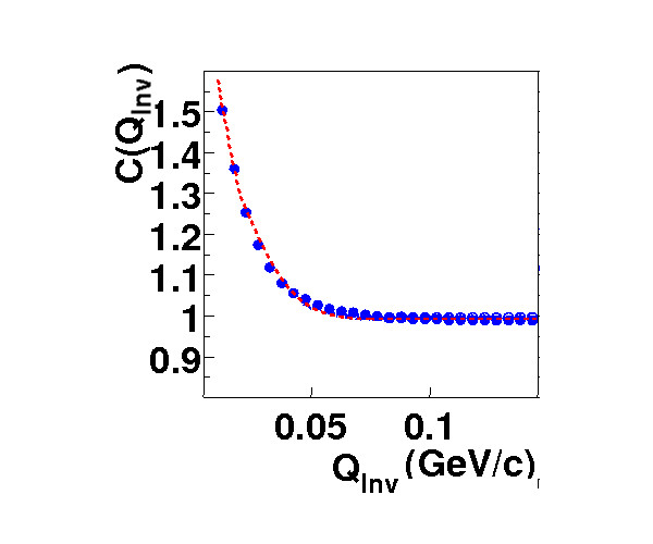
Obviously for $Q_{1}=Q_{2}$ both amplitudes are equal yielding the factor two on the right side. In the close by area the phase will usually change rapidly eliminating after averaging the interference contribution yielding the factor one. The resulting $Q_{1}=Q_{2}$ enhancement is observed experimentally as shown in figure 4. The chosen data are from the STAR collaboration. $Q_{inv}$ is the difference of the momenta in the center of mass system of the $\pi^{+}$’s. The normalization of the two particle spectrum $C(Q_{inv})$ uses an estimate obtained by mixing similar events. In the last 50 years there were many dozens of large collaborations seeing it. The observation of the statistical enhancement is text book level and beyond doubt kittel2005soft ; BEwiki .

x $\begin{array}[]{l}Q_{inv}=\\ \sqrt{(p_{1}-p_{2})^{2}-(E_{1}\text{-}E_{2})^{2}}\end{array}$ and $\begin{array}[]{l}C(Q_{inv})=\\ \rho_{2}(Q_{inv})/\rho_{2}^{reference}(Q_{inv})\end{array}$

Figure 4: The statistical enhancement

For central scattering the height of the emission area reflects the uncontracted size of the nuclei while the $\pi^{+}$-emission region is usually associated with individual nucleons determining it size. One can therefore select events for which one $\pi^{+}$ originates in the upper and one in the lower half. The particle emission is generally assumed to take less then $10\,\mathrm{fm}/c$ ferreres2018space ; andersson1986bose . The emission process is taken quantum mechanically, after emission particles are treated macroscopically.

The ,,crazy” observation appears in the following gedanken experiment (see figure 5). One considers an emission happening initially at $1fm/c$ with a Bose enhanced probability $\propto 2$. Later on at a time $1\,\mathrm{m}/c$ it is suddenly disturbed by a neutron at a suitable position so that the $\pi^{+}$ originating in the lower half independent of its momentum $Q_{1}$ or $Q_{2}$ will be absorbed. The interference enhancement is gone and the emission probability is now $\propto 1$. At times the emission has to be taken back. It means backward causation for a particular emission probability.

at $1~{}\mathrm{fm}/c$:

at $11~{}\mathrm{m}/c$:

Figure 5: Crazy gedanken experiment

The ontological reality of an emission and its probability can not questioned. So in this very special situation there is backward causation for real objects. The purpose of the Copenhagen interpretation was to avoid violations of causality. As it was not successful one has to abolish it. In a trade-off one can then accept ontological reality of wave functions and excepting their gauge part fields.

A critical ingredient in the argument is the assumption about the position of the transition from the quantum world to the macroscopic one (drawn as dash dotted line in the figures). As said, in particle physics the transition is usually taken as process dependent and the emission process itself is pictured as some kind of measurement procedure.

One way to escape the argument is to postpone the transition to the end of the process say to $11\mathrm{m}/c$. The problem is that there is an analogous astronomical Hanbury Brown - Twiss observation brown1957interferometry ; Bopp:2016nxn where the possible change in the set up corresponding to the neutron insertion can be light years away. The Copenhagen interpretation assumes that such a transition exists in a reasonable range and its exact position is not specified. However a year is clearly outside of the expectation of the Copenhagen interpretation closing the escape.

One somehow needs to develop a formalism where at least for a year most measurements in the star are somehow provisional. Also to introduce a rather arbitrary time scale for the transition seems unavoidable.

To argue for a simpler way out I reconsider the situation with measurements. Two central questions are:

What does the measurement have to do?

• Identify states originating in something like the ,,up” or ,,down” choice.

• Randomly elect the contributions from one choice.

• Delete the deselected contributions.

• Renormalize the selected one to get a unit probability.

When does the measurement has act?

• Outside the quantum domain behind the decoherence process.

• Witnesses have to be around encoding the measurement results.

To avoid the definition of limits I assume a finite life time of the universe $\tau_{\mathrm{final}}$.

2 Scenario with an extended final state

The survival time of witnesses is not fully appreciated. In truly ,,macroscopic” measurements some witnesses are around practically forever. In our finite universe this allows us to postpone measurements to the ,,end of the universe” $\tau_{\mathrm{final}}$ . In this way wave function collapses are completely avoided in the ,,physical” regions where one just has quantum dynamics.

The postponement relying on abundance of witnesses can be written as:

$$<i|\,U(t-t_{i})\,\mathcal{M}_{up}(t)\,U(\tau_{\mathrm{final}}-t)\,=<i|\,U(\tau_{\mathrm{final}}-t_{i})\,\mathcal{M}_{up-evolved}^{\prime}(\tau_{\mathrm{final}})$$ (2)

where $\mathcal{M}_{up}(t)$ is replaced by $\mathcal{M}_{up-evolved}^{\prime}(\tau_{\mathrm{final}})$. Here $\mathcal{M}$ stands just for the projection part, i.e. $M\mathcal{=M}\cdot N$ where $N$ is the normalization factor.

$-\tau_{\mathrm{final}}-$ $\uparrow$ $\tau$

Figure 6: Completely enclosed

To illustrate the situation one can consider Schrödingers cat. If the cruel experiment is done in a perfectly enclosed box all ergodicly accessible states will be visited before the end $\tau_{\mathrm{final}}$ is reached. There is no possibility that specific witnesses can have survived. In this way the final state can not select a unique macroscopic path way. Macroscopic dynamics is an approximation and in the considered situation coexisting macroscopic states have to be considered as a given.

How is it really?

$-\tau_{\mathrm{final}}-$ $\uparrow$ $\tau$ $\sim\sim\to$ some cm brain waves escape

Figure 7: Real box

Measurable radio frequency fields emitted from the brain indicate whether the cat is alive. Usually nobody talks about individual radio frequency photons. They carry an energy of something like unmeasurable $10^{-28}$ Joule.

Some of them will escape the box, the house, and the ionosphere to the dark sky eventually reaching the final state at $\tau_{\mathrm{final}}$ at which point a measurement can backward in time select the macroscopic path with an alive cat and deselect the one with a dead cat.

The exact value of the chosen scale $\tau_{\mathrm{final}}$ is not significant. Around $\tau_{\mathrm{final}}$ our universe is thin and rather non-interacting. So the witness evolution between $\tau_{\mathrm{final}}$ or $1000\,\tau_{\mathrm{final}}$ etc. is trivial. Obviously a scale choice discussed above is not avoided but now its value is irrelevant.

The resulting effective basic rules:

• Coexisting quantum pathways cannot be discerned and selected / deselected by a measurement at $\tau_{\mathrm{final}}$.

• For each and every macroscopic decision there are enough witnesses so that measurements at $\tau_{\mathrm{final}}$ can select / deselect it. In this way the complete, unique macroscopic path way is determined.

Definition of an effective final state density matrix:

With suitable boundary states density matrices one obtains:

$$\mathrm{probability}{}_{\mathcal{M}}=\frac{Tr(\rho_{i^{*},i}\,U(\tau_{f}-\tau_{i})\,\mathcal{M}^{\prime}\,\rho_{f,f^{*}}\,\mathcal{M}^{\prime}\,U^{*}(\tau_{f^{*}}-\tau_{i^{*}}))}{Tr(\rho_{i^{*},i}\,U(\tau_{f}-\tau_{i})\,\rho_{f,f^{*}}\,U^{*}(\tau_{f^{*}}-\tau_{i^{*}}))}$$ (3)

Defining $\widetilde{\rho_{f,f^{*}}}=\mathcal{M}^{\prime}\,\rho_{f,f^{*}}\,\mathcal{M}^{\prime}$ it simplifies.

Each of zillion branching of the macroscopic path way corresponds to a measurement decision which can be again and again be accounted for in this way by a change of the effective final density matrix finally yielding $\widetilde{\widetilde{\rho_{f,f^{*}}}}$ :

$$\mathrm{probability}{}_{\mathcal{M}}=\frac{Tr(\rho_{i^{*},i}\,U(\tau_{f}-\tau_{i})\,\widetilde{\widetilde{\rho_{f,f^{*}}}}\,U^{*}(\tau_{f^{*}}-\tau_{i^{*}}))}{Tr(\rho_{i^{*},i}\,U(\tau_{f}-\tau_{i})\,\rho_{f,f^{*}}\,U^{*}(\tau_{f^{*}}-\tau_{i^{*}}))}$$ (4)

The presented ,,two density matrices interpretation” is the simplest way fulfilling the requirements of discussed gedanken experiment. Also, its derivation did not involve speculative assumptions. To be convincing it should be useful to compare it with other interpretations.

Relationship to Everett’s Quantum Mechanics

In Everett’s QM all measurement options stay existing in a multiverse. The random physics decisions in measurements is replaced by a random association to observers which have witnessed the same quantum decisions. Our universe within the multiverse is defined by this community of observers we associate with.

Implicit is the assumption that observed universes can split as shown in figure 8 but that they never join. As in the two density matrices interpretation it requires an abundant existence of witnesses.

Figure 8: Everett’s tree

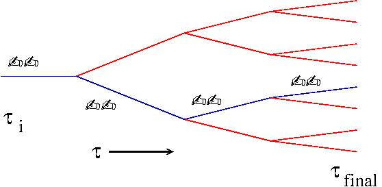
To have our universe defined up to $\tau_{\mathrm{final}}$ our community needs observers until that time. In principle these observers have access to all quantum decisions. They can therefore determine a density matrix consistent with all macroscopic decision. This allows then to macroscopically describe our universe in the multiverse in a two density matrix formalism. The fate of the multiverse outside of our universe shown in red in the figure is then irrelevant.

Relationship to Two State Vector Quantum Mechanics

Let us begin with the argument for the dominant state vector approximation. It is not rigorous as it requires the existence of a reasonably convergent expansion of the density matrix.

Without the normalization factor $N$ the effective final density matrix gets extremely tiny (something like $\sim 2^{-\#\,of\,all\,binary\,decisions}$). Expanding it:

$$\widetilde{\widetilde{\rho_{f,f^{*}}}} = c_{1}\cdot|f_{1}><f_{1}|+c_{2}\cdot|f_{2}><f_{2}|+c_{3}\cdot|f_{3}><f_{3}|\cdots$$ (5)

one finds something like $c_{1}\propto 2^{\mathrm{-huge}}$ and $c_{i}\propto 2^{\mathrm{-huge^{\prime}}}$. As $|\mathrm{huge}\mathrm{-huge}^{\prime}|$ is of order $\mathrm{huge}$ or$\mathrm{\sqrt{huge}}$ the largest term should suffice, i.e.:

$$\widetilde{\widetilde{\rho_{f,f^{*}}}} \approx c_{1}\cdot|\,f_{1}><f_{1}\,|~{}.$$ (6)

The approximation will be used in the following at several occasions. The simplification is also applied the initial state

$$\rho_{i,i^{*}}\,=|i><i|~{}.$$ (7)

In this way one obtains the Two State Vector description of Aharonov and collaborators aharonov1991complete ; aharonov2010time ; aharonov2017twotime . For simplicity I adhere in the following often to this Two State Vector description. The arguments can usually be transferred to the two density matrix description if the density matrices are constrained appropriately.

To obtain the Aharonov-Bergman-Lebowitz equation aharonov1964time one can take all macroscopic measurements in the universe as accounted for in $|f>$ except for an additional measurement $\mathcal{M}$:

$$\mathrm{probability}{}_{\mathcal{M}}=\frac{|\left[<i|U(\tau-\tau_{i})\,\mathcal{M}\,U(\tau_{f}-\tau)|f>\right]|^{2}}{|\left[<i|U(\tau_{f}-\tau_{i})|f>\right]|^{2}}\,.$$ (8)

The Two State Vector description was carefully investigated over many decades and no inconsistencies where found on the quantum side. However, the central question is how can a causal macroscopic dynamics follow from a non-causal quantum dynamics?

3 The time-ordered causal macroscopic dynamics

Figure 9: Decision tree

The considered gedanken experiments involved very special situations. True macroscopic measurements will approximately, somehow per definition average out enhancing and depleting phase effects. In Bopp:2016nxn I called this ,,correspondence transition rule”. It disallows direct macroscopic backward causation.

But what happens on a basic level? Causal macroscopic dynamics involves a decision tree shown in the figure 9. A decision at e.g. $D_{1}$ determines the future. How can a time symmetric non-causal theory underlie such a macroscopic causal decision tree with a time direction?

To explain the proposed mechanism one can start with a definition. The ,,Macroscopic State” $\{|q>\}$ is defined as sum/integral over all states macroscopically indistinguishable from the quantum state $|q>$:

$$\left\{|q>\right\}=\sum_{\mathrm{all\,states\,macroscopically\,consistent\,with\,}|q>}|q_{i}>$$ (9)

It includes all possible phases between different components and all unmeasurable individual low frequency photons etc. .

Figure 10: Macroscopic path ways

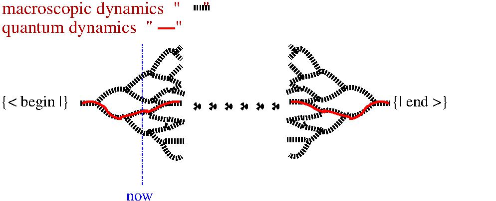
As said the full initial and final quantum states allows one single macroscopic path. What happens if one replaces the initial and final quantum state by Macroscopic States? Quantum decisions are often encoded in relative phases. With choices available the underlying QM now allows for many pathways consistent with the ,,macroscopic” initial and final states yielding a situation depicted in the figure 10.

The Macroscopic States somehow live in macroscopic dynamics. In purely macroscopic dynamics there would of course be one pathway from the initial to some final state. The splitting and joining in the figure is an effect of the underlying quantum dynamics. To avoid a contradiction to what is known in macroscopic dynamics one has to assume that the splitting and joining in the figure involves cosmologically long time scales. Macroscopic dynamics is only an empirical approximation which can be violated at untested scales.

Figure 11: Past evolution

The central assumption is our position in the universe. It is indicated by the dotted line in the figure 10. The source of the observed macroscopic causal time direction is the asymmetry of our position, i.e.:

$$\left(\tau_{\mathrm{now}}-\tau_{\mathrm{big\,bang}}\right)\ll\left(\tau_{\mathrm{\mathrm{final}}}-\tau_{\mathrm{now}}\right).$$

Figure 11 and 12 considers the resulting situation for both directions.

The past evolution is assumed to be too short to allow multiple pathways. With the known cosmic microwave background, with the known distribution of galaxies, and with the largely known astrophysical mechanisms the backward evolution is pretty much determined at least to up the freeze out. The hypothesis is that if all macroscopic details of the present universe - with all the atoms in all the stars in all the galaxies - would be known the past could be determined in an essentially in-ambiguous way.

Figure 12: Future evolution

The situation of the future is assumed to be long enough to allow for multiple pathways. Allow for an anthropogenic picture in which decisions are usually considered. Driving on the highway one can turn right to Dortmund or left to Frankfurt and one can make a mess in Frankfurt and this will have obvious consequences afterward. That the fixed final macroscopic state at the end of the universe limits what can possibly be done is of no practically concern.

In reality the present and final boundary states are quantum states which yield a uniquely determined macroscopic path way. All decisions are actually encoded in the final state which obviously can not contain a time direction. That they happen at the bifurcation points denoted by ,,D” is an illusion faking the causal direction.

Problems with the fully deterministic fixed final state model:

The argumentation for a final state model is convincing and there are no intrinsic paradoxes. But some aspects of fixed final state model are hard to agree to:

$\bullet$   Willful agents cannot exist!

Within the considered framework a willful agent had to adjust the fixed final state at the end of the universe in an incalculable way. To avoid recalculating the universe one has to drop the concept of willful agents but this is hard to accept hossenfelder2019rethinking . It is not just philosophical. Consider a seminar. Without a willful chair a speaker could go on forever.

The second problem is more on an esthetic level.

$\bullet$   The fixed randomness within the final state!

To maintain Born’s Rule the final state can not bias quantum decisions. It has to be fixed in a random way which is clearly uglier done within such a detached state than the random decisions during measurement processes.

4 The matching state

There is an appealing way out. So far we mainly considered the evolution of wave functions or fields. Physics depends on them and their conjugate. To allow for external manipulations one can consider the quantum world and its conjugate separately with distinct initial values and replace both fixed final states by a common matching one.

An external agent lives in the macroscopic world. He can manipulate the wave functions or fields and their conjugates at a given time. The matching final state will change by itself accordingly. No incalculable action of the agent is required.

To avoid arbitrary assumptions about the time and nature of the matching I turn to a simple cosmological big-bang / big-crunch scenario. It allows for a simple implementation of the bidirectional concept. It is, however, not absolutely essential for the concept.

5 The bidirectional big-bang / big-crunch scenario

There are many exciting new observation in cosmology and astrophysics. Extrapolating observations it is usually assumed that a rather but not completely homogenous universe undergoes an accelerating expansion. The central argument for macroscopic causality required that the total life time of the universe has to be much larger than its present age. In this way extrapolations of present observation are not really relevant.

The understanding of dark energy or what ever drives the dynamic of the cosmos is not jet available di2019planck ; kaloper2015sequestration . The concept that eventually the anti-gravitating dark energy gets exhausted leading to a big bang / big crunch universe is at least appealing.

Of course there are black holes and the structure of the universe must be topologically intricate. The expectation is that these complications are not relevant for the basic understanding of our epoch and that one can consider a simple most configuration where the total age of the universe is $\tau$ and both the expanding and the contracting phase last for $\tau/2$ .

The initial and final state are not be CPT conjugates. As above all quantum decisions are stored in the initial and final state. Their overlap:

$$<\mathrm{bang}\,|\,\mathrm{crunch}>=\left(\begin{array}[]{c}\mathrm{extremely}\\ \mathrm{tiny}\end{array}\right)$$ (10)

is again something like $2^{-\#\,\mathrm{all\,decisions\,in\,both\,directions}}$ ignoring weights and non binary branching.

It also holds for the overlap of the unitarily evolved states just before and just after this ,,border” state of maximum extend. No ,,fine tuning” is involved as no big number is created dynamically. At the border the extremely extended universe has only a tiny fraction of occupied states. So matching is extremely rare. Both strongly entangled evolved states should miss common entanglements simply for statistical reasons. Coexisting path ways involving the expanding and contracting phases are practically excluded.

For the state of maximum extend one can define something like density function connecting the incoming and outgoing states:

$$\rho_{\mathrm{max.\,extend}}=\sum_{i,j}\rho(i,j)\,|\begin{array}[]{c}\mathrm{max.}\\ \mathrm{extend}\end{array}(i)><\begin{array}[]{c}\mathrm{max.}\\ \mathrm{extend}\end{array}(j)|$$ (11)

As the Hamiltonian describing the evolution involves a Hermitian matrix $\rho_{\mathrm{max.\,extend}}$ is diagonalizable. With the dominant state argument its extreme smallness means that typically only a single component dominates, i.e. one can just approximate it as:

$$\rho_{\mathrm{max.\,extend}}\sim|\mathrm{border}><\mathrm{border|}\,.$$ (12)

For the total evolution it leaves two factors:

$$<\mathrm{bang}\,|\,U\,|\,\mathrm{border}>\otimes<\mathrm{border\,|}\,U\,\mathrm{|\,crunch}>$$ (13)

No time arrow is accepted, so the expanding world is analogous to the contracting one. For both the ,,expanding” and the ,,contracting” phases the border state is an effective final quantum state determining the macroscopic path ways in its neighborhood as argued in section 2. The criterion was that witnesses can reach it. The neighborhood is assumed to cover much of the universe including our epoch.

In this region the common quantum border state has the consequence:

The expanding and contracting worlds
are macroscopically identical.

This result allows an obvious interpretation:

Surjection hypothesis

To avoid strange partnerships one postulates:

• The quantum states are defined in $[0,\tau]$.

• Macroscopic dynamics is taken to extend from $[0,\tau/2]$.

Macroscopic objects (like us) then live

• with their wave function $\psi(t)$ in the ,,expanding” phase $[0,\tau/2]$,

• with their conjugate one $\psi(\tau-t)^{CPT}$ in the ,,contracting” phase $[\tau/2,\tau]$.

The proposition has a number of attractive consequences which makes it quite appealing.

A will-full agent is now possible.

At the macroscopic time $t$ corresponding to the quantum times $t$ and $\tau-t$ a manipulating agent can introduce unitary operators:

$$\psi(t) \longmapsto \widetilde{\psi}(t+\epsilon)=\mathrm{Operator}[\psi(t)]$$

$$\psi(\tau-t) \longmapsto \widetilde{\psi}(\tau-t-\epsilon)=\mathrm{Operator^{CPT}}[\psi(\tau-t)]$$ (14)

In the macroscopic future $[t,\tau-t]$ the wave functions change and a new border component will dominate:

$$\psi(\mathrm{border})\longmapsto\widetilde{\psi}(\mathrm{border})$$ (15)

automatically reflecting the manipulation. No unusual action of the agent is required.

The manipulation of the agent does not introduce a fundamentally new time direction. The changed matching can in principle affect the contributing wave functions also in the macroscopic past. However as $t\ll\tau$ the functions $\psi(t^{\prime}<t)$ and $\psi(t^{\prime}>\tau-t)$ stay practically unchanged.

Stern-Gerlach experiment

An agent can prepare a ,,Stern-Gerlach experiment” shown in figure 13.

Figure 13: Bidirectional Stern-Gerlach measurement

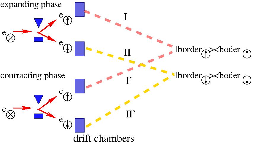
As the drift chambers create macroscopic traces with a large number of witnesses mixed ,,up”/”down” contributions are excluded leaving the red or yellow contributions.

One can now compare the red and yellow contributions:

$$\mathrm{contributions} \propto\begin{cases}\begin{array}[]{ccc}2^{-\mathrm{decision\,on\,paths\,I\,and\,I^{\prime}}}&=&2^{-huge}\\ 2^{-\mathrm{decision\,on\,paths\,II\,and\,II^{\prime}}}&=&2^{-huge^{\prime}}\end{array}\end{cases}$$ (16)

Statistically one contribution will completely dominate. The choice reflects unknown properties of the available future path. The randomness disliked by Einstein found a fundamentally deterministic explanation.

As it is well known the quantum randomness gets lost in the macroscopic world just by statistics as large numbers (like Avogadro’s) are involved. As there are no correlations between the considered ensemble and the future path ways the effective randomness obtained suffices for this purpose.

In an average both possibilities are equal, i.e.:

$$\mathrm{probability}\left(huge>huge^{\prime}\right)=\mathrm{probability}\left(huge<huge^{\prime}\right)$$ (17)

which has the consequence:

$$\begin{array}[]{ccccc}\mathrm{prob.}\left[e_{\,\uparrow}\,\right]&=&\left(\begin{array}[]{c}expanding\\ component\end{array}\right)\cdot\left(\begin{array}[]{c}contracting\\ component\end{array}\right)&=&\left|<e_{\otimes}\,|\,e_{\,\uparrow}\,{>}\right|^{2}\\ \mathrm{prob.}\left[e_{\,\downarrow}\,\right]&=&\left(\begin{array}[]{c}expanding\\ component\end{array}\right)\cdot\left(\begin{array}[]{c}contracting\\ component\end{array}\right)&=&\left|<e_{\otimes}\,|\,e_{\,\downarrow}\,{>}\right|^{2}\end{array}$$ (18)

It means the ,,Born rule” holds vaidman2019derivations . The squares brackets on the right are no longer chosen as they have the required properties but they are now a direct consequence of the physical process.

6 Important cosmological consequences

In the cosmological development there can be special situations or early periods where the remoteness of the final state does not allow a macroscopic description and the needed difference between the initial bang and the final crunch state will get important.

The possible absence of a macroscopic description demystifies paradoxes. In a closed box Schrödingers cat can be dead and alive. The same applies for the grandpa in a general relativity loop used in arguments discrediting backward causation.

It also could affect the view of the early cosmological development. Before QED freeze out the universe is heavily interacting and it is to be expected that there are sooner or later no longer surviving witnesses to fix a unique macroscopic path way to eliminate macroscopic coexistence.

A macroscopic description of the earlier universe could be unacceptable. Even to use a unique macroscopic Hubble parameter H(t) as it used in the Friedman - equations might be questionable.

Homogeneity of the early universe

The transition from a period without a macroscopic description to a macroscopic one requires special considerations. There is a simple observation about contributing path ways. Unusual components of the quantum phase will be deselected and only components close to the average will collectively produce a significant contribution entering the macroscopic phase. In this way a homogeneous contribution at the transition point is strongly favored.

The initial big bang state in the argument for macroscopic causality can be replaced in this framework by this initial homogeneous state. The basic initial state / border state asymmetry needed for the argument stays.

The universe is actually more homogeneous then expected from simple estimates guth1981inflationary . It is usually attributed to a limited horizon caused by a rapid expansion of the universe due to inflation. The concept might offer a way to avoid the complicated requirements of inflation models.

Inflation models have according to a recent work of Chowdhury et al. chowdhury2019inflation a serious fundamental problem within the Copenhagen quantum mechanics. One needs to come from an initially coherent state to one allowing for temperature fluctuations. Quantum jumps would do the trick but they are not possible in inflation models as the universe is taken as a closed system without an external observational macroscopic entity.

Summary

Quantum statistical effects strongly suggest to abolish causality on the quantum side and to find arguments to effectively resurrect it in the macroscopic world.

In a universe with a finite life time $\tau_{\mathrm{final}}$ sufficiently abundant witnesses can make it possible to postpone all measurements to $\tau_{\mathrm{final}}$ where they then can be incorporated in an effective final density matrix. The resulting completely deterministic concept with a fixed initial and a fixed final density matrix is closely related to the Two State Vector quantum mechanics of Aharonov and coworkers and a universe in the Everett multiversum inhabited by a final observer our community in our universe associate with.

As it stands the concept is not acceptable. Free macroscopic agents are indispensable. A simple way to incorporate free will is to turn to a slightly modified model in which the fields and their conjugates evolve independently and replace the fixed final state on each side by a matching common one. To avoid ad hoc assumptions about the matching a big bang / big crunch cosmology is chosen with an expanding and a contracting quantum phase. A free agent then lives - like all macroscopic objects - with the wave function in the expanding part and with the complex conjugate one in the contracting part. Operators he is allowed to enter on both sides will effect the evolution in between, i.e. in the macroscopic future.

To conclude I obtained a concept that has no intrinsic paradoxes and allows for free agents. Unfortunately it requires to abandon concepts many people are not willing to question.