Hyperasymptotic approximation to the top, bottom and charm pole mass

Cesar Ayala Department of Physics, Universidad Técnica Federico Santa María (UTFSM), Casilla 110-V, Valparaíso, Chile    Xabier Lobregat    Antonio Pineda Grup de Física Teòrica, Dept. Física and IFAE-BIST, Universitat Autònoma de Barcelona,
E-08193 Bellaterra (Barcelona), Spain
Abstract

We construct hyperasymptotic expansions for the heavy quark pole mass regulated using the principal value (PV) prescription. We apply such hyperasymptotic expansions to the B/D𝐵𝐷B/D meson masses, and Λ¯¯Λ\bar{\Lambda} computed in the lattice. The issue of the uncertainty of the (top) pole mass is critically reexamined. The present theoretical uncertainty in the relation between m¯tsubscript¯𝑚𝑡{\overline{m}}_{t}, the MS¯¯MS\overline{\rm MS} top mass, and mt,PVsubscript𝑚𝑡PVm_{t,\rm PV}, the top pole mass regulated using the PV prescription, is numerically assessed to be δmt,PV=28MeV𝛿subscript𝑚𝑡PV28MeV\delta m_{t,\rm PV}=28\;{\rm MeV} for m¯t=163subscript¯𝑚𝑡163{\overline{m}}_{t}=163 GeV.

I Introduction

We construct hyperasymptotic expansions for the heavy quark pole mass regulated using the principal value (PV) prescription along the lines of HyperI . We generalize the discussion of that reference by including possible ultraviolet renormalons. We then apply such expansions to various observables. The name hyperasymptotic we borrow from BerryandHowls . For a treatise of hyperasymptotic expansions in the context of ordinary differential equations see Boyd99 .

In HyperI we studied observables characterized by having a large scale QΛQCDmuch-greater-than𝑄subscriptΛQCDQ\gg\Lambda_{\rm QCD}, and for which the operator product expansion (OPE) is believed to be a good approximation. We computed them within an hyperasymptotic expansion. More specifically, the perturbative part of the OPE was summed up using the PV prescription: SPVsubscript𝑆PVS_{\rm PV}. The difference between SPVsubscript𝑆PVS_{\rm PV} and the full non-perturbative (NP) result is assumed to exactly scale as the intrinsic NP terms of the OPE. In general terms:

Observable(QΛQCD)=SPV(αX(Q))+KX(PV)αXγ(Q)ΛXdQd(1+𝒪(αX(Q)))+𝒪(ΛXdQd),Observable𝑄subscriptΛQCDsubscript𝑆PVsubscript𝛼𝑋𝑄superscriptsubscript𝐾𝑋PVsuperscriptsubscript𝛼𝑋𝛾𝑄superscriptsubscriptΛ𝑋𝑑superscript𝑄𝑑1𝒪subscript𝛼𝑋𝑄𝒪superscriptsubscriptΛ𝑋superscript𝑑superscript𝑄superscript𝑑{\rm Observable}(\frac{Q}{\Lambda_{\rm QCD}})=S_{\rm PV}(\alpha_{X}(Q))+K_{X}^{\rm(PV)}\alpha_{X}^{\gamma}(Q)\frac{\Lambda_{X}^{d}}{Q^{d}}\left(1+{\cal O}(\alpha_{X}(Q))\right)+{\cal O}(\frac{\Lambda_{X}^{d^{\prime}}}{Q^{d^{\prime}}})\,, (1)

where the last term refers to genuine higher order terms in the OPE (d>d>0superscript𝑑𝑑0d^{\prime}>d>0). Then, since SPVsubscript𝑆PVS_{\rm PV} can not be computed exactly, we obtain it approximately along an hyperasymptotic expansion (a combination of (truncated) perturbative sums and of NP corrections). This is possible if enough terms of the perturbative expansion are known, and if the divergent structure of the leading renormalons of the observable is also known. This allows us to have a clear (parametric) control on the error of the computation. Two alternative methods were considered in HyperI depending on how the truncation of the leading perturbative sum

ST(α)=n=0Npn(X)αXn+1(μ)subscript𝑆𝑇𝛼superscriptsubscript𝑛0𝑁subscriptsuperscript𝑝𝑋𝑛superscriptsubscript𝛼𝑋𝑛1𝜇S_{T}(\alpha)=\sum_{n=0}^{N}p^{(X)}_{n}\alpha_{X}^{n+1}(\mu) (2)

is made:

  1. 1)

    N𝑁N and μQsimilar-to𝜇𝑄\mu\sim Q large but finite:

    N=NP|d|2πβ0αX(μ)(1cαX(μ)),𝑁subscript𝑁𝑃𝑑2𝜋subscript𝛽0subscript𝛼𝑋𝜇1𝑐subscript𝛼𝑋𝜇N=N_{P}\equiv|d|\frac{2\pi}{\beta_{0}\alpha_{X}(\mu)}\big{(}1-c\,\alpha_{X}(\mu)\big{)}\,, (3)
  2. 2)

    N𝑁N\rightarrow\infty and μ𝜇\mu\rightarrow\infty in a correlated way. We considered two options:

    A)N+1=NS(α)|d|2πβ0αX(μ);B)N=NA(α)|d|2πβ0αX(μ)(1cαX(Q)){\rm A)}\quad N+1=N_{S}(\alpha)\equiv|d|\frac{2\pi}{\beta_{0}\alpha_{X}(\mu)}\,;\qquad{\rm B)}\quad N=N_{A}(\alpha)\equiv|d|\frac{2\pi}{\beta_{0}\alpha_{X}(\mu)}\big{(}1-c^{\prime}\alpha_{X}(Q)\big{)} (4)

where c>0superscript𝑐0c^{\prime}>0 but c𝑐c is arbitrary otherwise. Note that in case 1), c𝑐c can partially simulate changes on the scale or scheme of αXsubscript𝛼𝑋\alpha_{X}. d𝑑d is the dimension associated to a given renormalon. Note that in this paper d𝑑d can be positive (infrared renormalons) or negative (ultraviolet renormalons), unlike in HyperI , where only positive d𝑑d’s were considered. Note also that genuine NP corrections are only associated to positive d𝑑d’s.

We will not study the modifications the inclusion of ultraviolet renormalons produce in case 2). In this paper we are mainly concerned in the scenario where the leading renormalon is of infrared nature and subleading renormalons can be ultraviolet and/or infrared. This is the case of the pole mass. In such scenario the precision we can obtain in case 2) is limited by the approximate knowledge of the leading infrared renormalon and we cannot add further to the discussion given in HyperI . Different is the case 1), which we discuss in the next section.

The structure of the paper is as follows. In Sec. II we review the general case. Compared with HyperI we include the possible effect of ultraviolet renormalons. In Sec. III we study the pole mass of a heavy quark in the large β0subscript𝛽0\beta_{0} approximation. We use it as toy-model to test our methods. We then move to real QCD. In Sec. IV we study the B/D𝐵𝐷B/D meson mass and lattice evaluations of Λ¯¯Λ\bar{\Lambda}. Finally, in Sec. V we do a dedicated study of the top mass.

In general we will avoid to make explicit the scheme (X𝑋X) and scale (μ𝜇\mu) dependence unless necessary.

II General formulas

II.1 N𝑁N large and μQΛQCDsimilar-to𝜇𝑄much-greater-thansubscriptΛQCD\mu\sim Q\gg\Lambda_{\rm QCD}. Eq. (3). Case 1)

This case was already discussed at length in HyperI . We now give the general expression after the inclusion of ultraviolet renormalons (for a more detailed discussion see Ayala:2019lak ). It can be written in the following way

SPV(Q)=SP+{|d|}S|d|+{d>0}Ωd+{d<0}Ωd,subscript𝑆PV𝑄subscript𝑆𝑃subscript𝑑subscript𝑆𝑑subscript𝑑0subscriptΩ𝑑subscript𝑑0subscriptΩ𝑑S_{\rm PV}(Q)=S_{P}+\sum_{\{|d|\}}S_{|d|}+\sum_{\{d>0\}}\Omega_{d}+\sum_{\{d<0\}}\Omega_{d}\,, (5)

where

SPn=0NP(|dmin|)pnαn+1(μ)S|d|=0,subscript𝑆𝑃superscriptsubscript𝑛0subscript𝑁𝑃subscript𝑑𝑚𝑖𝑛subscript𝑝𝑛superscript𝛼𝑛1𝜇subscript𝑆𝑑0S_{P}\equiv\sum_{n=0}^{N_{P}(|d_{min}|)}p_{n}\alpha^{n+1}(\mu)\equiv S_{|d|=0}\,, (6)

and (|d|>0𝑑0|d|>0)

S|d|n=NP(|d|)+1NP(|d|)(pnpn(as))αn+1(μ),subscript𝑆𝑑superscriptsubscript𝑛subscript𝑁𝑃𝑑1subscript𝑁𝑃superscript𝑑subscript𝑝𝑛superscriptsubscript𝑝𝑛𝑎𝑠superscript𝛼𝑛1𝜇S_{|d|}\equiv\sum_{n=N_{P}(|d|)+1}^{N_{P}(|d^{\prime}|)}(p_{n}-p_{n}^{(as)})\alpha^{n+1}(\mu)\,, (7)

where the asymptotic behavior associated to renormalons with dimensions |d|absent𝑑\leq|d| is included in pn(as)superscriptsubscript𝑝𝑛𝑎𝑠p_{n}^{(as)}, and dsuperscript𝑑d^{\prime} is the dimension of the closest renormalon to the origin in the Borel plane fulfilling that |d|>|d|superscript𝑑𝑑|d^{\prime}|>|d|. ΩdsubscriptΩ𝑑\Omega_{d} is a modification of the definition of terminant given in Dingle that is more suitable to our case. Whereas in Dingle (pNαN×p_{N}\alpha^{N}\times the) terminant refers to the completation of the superasymptotic approximation to give the complete result, here ΩdsubscriptΩ𝑑\Omega_{d} is the completion of the part of the perturbative series associated to the singularity located at uβ0t4π=d2𝑢subscript𝛽0𝑡4𝜋𝑑2u\equiv\frac{\beta_{0}t}{4\pi}=\frac{d}{2} in the Borel plane using the PV prescription. For the case of infrared renormalons (d>0𝑑0d>0) the general analytic expression of ΩdsubscriptΩ𝑑\Omega_{d} can be found in HyperI . For a generic ultraviolet renormalon (d<0𝑑0d<0) that produces the asymptotic behavior

pn(as)=ZOdXμdQdΓ(n+b+1)Γ(b+1)(β02πd)n{1+c1bn+b+c2b2(n+b)(n+b1)+},superscriptsubscript𝑝𝑛𝑎𝑠superscriptsubscript𝑍subscript𝑂𝑑𝑋superscript𝜇𝑑superscript𝑄𝑑Γ𝑛superscript𝑏1Γsuperscript𝑏1superscriptsubscript𝛽02𝜋𝑑𝑛1subscript𝑐1superscript𝑏𝑛superscript𝑏subscript𝑐2superscript𝑏2𝑛superscript𝑏𝑛superscript𝑏1p_{n}^{(as)}=Z_{O_{d}}^{X}\frac{\mu^{d}}{Q^{d}}\frac{\Gamma(n+b^{\prime}+1)}{\Gamma(b^{\prime}+1)}\left(\frac{\beta_{0}}{2\pi d}\right)^{n}\bigg{\{}1+c_{1}\frac{b^{\prime}}{n+b^{\prime}}+c_{2}\frac{b^{\prime 2}}{(n+b^{\prime})(n+b^{\prime}-1)}+\dots\bigg{\}}\,, (8)

Ωd<0subscriptΩ𝑑0\Omega_{d<0} reads

Ωd<0=ΔΩUV(db)+c1ΔΩUV(db1)+,subscriptΩ𝑑0ΔsubscriptΩ𝑈𝑉𝑑𝑏subscript𝑐1ΔsubscriptΩ𝑈𝑉𝑑𝑏1\Omega_{d<0}=\Delta\Omega_{UV}(db)+c_{1}\Delta\Omega_{UV}(db-1)+\cdots\,, (9)

where111An sketch of how these computations are done is given in Appendix A. (we define ηcb+2π|d|cβ01subscript𝜂𝑐superscript𝑏2𝜋𝑑𝑐subscript𝛽01\eta_{c}\equiv-b^{\prime}+\frac{2\pi|d|c}{\beta_{0}}-1 where b=dbγsuperscript𝑏𝑑𝑏𝛾b^{\prime}=db-\gamma)

ΔΩUV(db)ΔsubscriptΩ𝑈𝑉𝑑𝑏\displaystyle\Delta\Omega_{UV}(db) =\displaystyle= ZOdXμdQd(1)NP+11Γ(b+1)(β02π|d|)NP+1αNP+20𝑑xexxNP+1+b1+xβ0α2π|d|superscriptsubscript𝑍subscript𝑂𝑑𝑋superscript𝜇𝑑superscript𝑄𝑑superscript1subscript𝑁𝑃11Γsuperscript𝑏1superscriptsubscript𝛽02𝜋𝑑subscript𝑁𝑃1superscript𝛼subscript𝑁𝑃2superscriptsubscript0differential-d𝑥superscript𝑒𝑥superscript𝑥subscript𝑁𝑃1superscript𝑏1𝑥subscript𝛽0𝛼2𝜋𝑑\displaystyle Z_{O_{d}}^{X}\frac{\mu^{d}}{Q^{d}}(-1)^{N_{P}+1}\frac{1}{\Gamma(b^{\prime}+1)}\left(\frac{\beta_{0}}{2\pi|d|}\right)^{N_{P}+1}\alpha^{N_{P}+2}\int_{0}^{\infty}dx\,\frac{e^{-x}x^{N_{P}+1+b^{\prime}}}{1+\frac{x\beta_{0}\alpha}{2\pi|d|}}
=\displaystyle= ZOdXμdQd(1)NP+1πΓ(b+1)(β0|d|)b1/2α(μ)1/2be2π|d|β0α(μ){1\displaystyle Z_{O_{d}}^{X}\frac{\mu^{d}}{Q^{d}}(-1)^{N_{P}+1}\frac{\pi}{\Gamma(b^{\prime}+1)}\left(\frac{\beta_{0}}{|d|}\right)^{-b^{\prime}-1/2}\alpha(\mu)^{1/2-b^{\prime}}e^{\frac{-2\pi|d|}{\beta_{0}\alpha(\mu)}}\bigg{\{}1
+α(μ)πβ012|d|[1+3ηc2]𝛼𝜇𝜋subscript𝛽012𝑑delimited-[]13superscriptsubscript𝜂𝑐2\displaystyle+\frac{\alpha(\mu)}{\pi}\frac{\beta_{0}}{12|d|}\left[-1+3\eta_{c}^{2}\right]
+α2(μ)π2β021152|d|2[1348ηc60ηc2+48ηc3+36ηc4]+𝒪(α3)}.\displaystyle+\frac{\alpha^{2}(\mu)}{\pi^{2}}\frac{\beta_{0}^{2}}{1152|d|^{2}}\bigg{[}13-48\eta_{c}-60\eta_{c}^{2}+48\eta_{c}^{3}+36\eta_{c}^{4}\bigg{]}+\mathcal{O}(\alpha^{3})\bigg{\}}\,.

Joining all terms together we have

Ωd<0=α(μ)KX(P)Q|d|μ|d|e2π|d|β0α(μ)(β0α(μ)4π)b{1+K¯X,1(P)α(μ)+K¯X,2(P)α2(μ)+𝒪(α3(μ))},subscriptΩ𝑑0𝛼𝜇superscriptsubscript𝐾𝑋𝑃superscript𝑄𝑑superscript𝜇𝑑superscript𝑒2𝜋𝑑subscript𝛽0𝛼𝜇superscriptsubscript𝛽0𝛼𝜇4𝜋superscript𝑏1superscriptsubscript¯𝐾𝑋1𝑃𝛼𝜇superscriptsubscript¯𝐾𝑋2𝑃superscript𝛼2𝜇𝒪superscript𝛼3𝜇\Omega_{d<0}=\sqrt{\alpha(\mu)}K_{X}^{(P)}\frac{Q^{|d|}}{\mu^{|d|}}e^{\frac{-2\pi|d|}{\beta_{0}\alpha(\mu)}}\left(\frac{\beta_{0}\alpha(\mu)}{4\pi}\right)^{-b^{\prime}}\bigg{\{}1+\bar{K}_{X,1}^{(P)}\alpha(\mu)+\bar{K}_{X,2}^{(P)}\alpha^{2}(\mu)+\mathcal{O}\left(\alpha^{3}(\mu)\right)\bigg{\}}\,, (11)

where

KX(P)superscriptsubscript𝐾𝑋𝑃\displaystyle K_{X}^{(P)} \displaystyle\equiv Z𝒪dX(1)Np+1(β0π2|d|)1/21Γ(b+1)(2|d|)b,subscriptsuperscript𝑍𝑋subscript𝒪𝑑superscript1subscript𝑁𝑝1superscriptsubscript𝛽0superscript𝜋2𝑑121Γsuperscript𝑏1superscript2𝑑superscript𝑏\displaystyle Z^{X}_{\mathcal{O}_{d}}(-1)^{N_{p}+1}\left(\frac{\beta_{0}}{\pi^{2}|d|}\right)^{-1/2}\frac{1}{\Gamma(b^{\prime}+1)}\left(\frac{2}{|d|}\right)^{-b^{\prime}}\,, (12)
K¯X,1(P)superscriptsubscript¯𝐾𝑋1𝑃\displaystyle\bar{K}_{X,1}^{(P)} \displaystyle\equiv (2π)1/2(c1β0b22π|d|+β012|d|2π(1+3ηc2)),superscript2𝜋12subscript𝑐1subscript𝛽0superscript𝑏22𝜋𝑑subscript𝛽012𝑑2𝜋13superscriptsubscript𝜂𝑐2\displaystyle\left(\frac{2}{\pi}\right)^{1/2}\left(c_{1}\frac{\beta_{0}b^{\prime}}{2\sqrt{2\pi}|d|}+\frac{\beta_{0}}{12|d|\sqrt{2\pi}}(-1+3\eta_{c}^{2})\right)\,, (13)
K¯X,2(P)superscriptsubscript¯𝐾𝑋2𝑃\displaystyle\bar{K}_{X,2}^{(P)} \displaystyle\equiv (2π)1/2(c2b2β0242|d|2π3/2+c1bβ02(1+3(ηc+1)2)242|d|2π3/2\displaystyle\left(\frac{2}{\pi}\right)^{1/2}\bigg{(}c_{2}\frac{b^{\prime 2}\beta_{0}^{2}}{4\sqrt{2}|d|^{2}\pi^{3/2}}+c_{1}\frac{b^{\prime}\beta_{0}^{2}(-1+3(\eta_{c}+1)^{2})}{24\sqrt{2}|d|^{2}\pi^{3/2}} (14)
+β021152|d|221/2π3/2[1348ηc60ηc2+48ηc3+36ηc4]).\displaystyle+\frac{\beta_{0}^{2}}{1152|d|^{2}2^{1/2}\pi^{3/2}}\bigg{[}13-48\eta_{c}-60\eta_{c}^{2}+48\eta_{c}^{3}+36\eta_{c}^{4}\bigg{]}\bigg{)}\,.

Note that in this case μ𝜇\mu is in the denominator. If we set the anomalous dimension to zero (b=dbsuperscript𝑏𝑑𝑏b^{\prime}=db), Ωd<0α(μ)ΛQCD|d|Q|d|μ2|d|similar-tosubscriptΩ𝑑0𝛼𝜇superscriptsubscriptΛQCD𝑑superscript𝑄𝑑superscript𝜇2𝑑\Omega_{d<0}\sim\sqrt{\alpha(\mu)}\frac{\Lambda_{\rm QCD}^{|d|}Q^{|d|}}{\mu^{2|d|}} (unlike for infrared renormalons where Ωd>0α(μ)ΛQCDdQdsimilar-tosubscriptΩ𝑑0𝛼𝜇superscriptsubscriptΛQCD𝑑superscript𝑄𝑑\Omega_{d>0}\sim\sqrt{\alpha(\mu)}\frac{\Lambda_{\rm QCD}^{d}}{Q^{d}}). If one takes μ𝜇\mu very large this term will be quite small. In practice, if we take μQsimilar-to𝜇𝑄\mu\sim Q, we may need this term.

SPVsubscript𝑆PVS_{\rm PV} will be computed truncating the hyperasymptotic expansion in a systematic way. This means truncating Eq. (5) as follows (note that we always define D𝐷D to be positive):

SPV(D,N)(Q)subscriptsuperscript𝑆𝐷𝑁PV𝑄\displaystyle S^{(D,N)}_{\rm PV}(Q) =\displaystyle= {|d|}S|d|<D+{|d|D}Ωdsubscript𝑑subscript𝑆𝑑𝐷subscript𝑑𝐷subscriptΩ𝑑\displaystyle\sum_{\{|d|\}}S_{|d|<D}+\sum_{\{|d|\leq D\}}\Omega_{d}
+n=NP(D)+1NP(D)+N(pnpn(as))αn+1(μ).superscriptsubscript𝑛subscript𝑁𝑃𝐷1subscript𝑁𝑃𝐷𝑁subscript𝑝𝑛superscriptsubscript𝑝𝑛𝑎𝑠superscript𝛼𝑛1𝜇\displaystyle+\sum_{n=N_{P}(D)+1}^{N_{P}(D)+N}(p_{n}-p_{n}^{(as)})\alpha^{n+1}(\mu)\,.

For each value of the couple (D,N)𝐷𝑁(D,N), we can state the parametric accuracy of SPV(D,N)(Q)subscriptsuperscript𝑆𝐷𝑁PV𝑄S^{(D,N)}_{\rm PV}(Q). For instance for S(0,NP)superscript𝑆0subscript𝑁𝑃S^{(0,N_{P})} the error would be (up to a numerical and a αXsubscript𝛼𝑋\sqrt{\alpha_{X}} factor)

δS(0,NP)𝒪(e|dmin|2πβ0αX(Q)).similar-to𝛿superscript𝑆0subscript𝑁𝑃𝒪superscript𝑒subscript𝑑𝑚𝑖𝑛2𝜋subscript𝛽0subscript𝛼𝑋𝑄\delta S^{(0,N_{P})}\sim{\cal O}\left(e^{-|d_{min}|\frac{2\pi}{\beta_{0}\alpha_{X}(Q)}}\right)\,. (16)

This is what is commonly named the superasymptotic approximation. For S(|dmin|,0)superscript𝑆subscript𝑑𝑚𝑖𝑛0S^{(|d_{min}|,0)} the parametric form of the error reads (up to a numerical and a possible αX3/2subscriptsuperscript𝛼32𝑋\alpha^{3/2}_{X} factor):

δS(|dmin|,0)𝒪(e|dmin|2πβ0αX(Q)(1+ln(|d/dmin|)),\delta S^{(|d_{min}|,0)}\sim{\cal O}\left(e^{-|d_{min}|\frac{2\pi}{\beta_{0}\alpha_{X}(Q)}\left(1+\ln(|d/d_{min}|\right)}\right)\,, (17)

where d𝑑d is the location of the next renormalon closest to the origin. This corresponds to the first term in the hyperasymptotic approximation. The expression for the error in the general case SPV(D,N)(Q)subscriptsuperscript𝑆𝐷𝑁PV𝑄S^{(D,N)}_{\rm PV}(Q) reads (NNP𝑁subscript𝑁𝑃N\not=N_{P} but large)

δS(D,N)𝒪(eD2πβ0αX(Q)(1+ln(|d/D|)αXN),\delta S^{(D,N)}\sim{\cal O}\left(e^{-D\frac{2\pi}{\beta_{0}\alpha_{X}(Q)}\left(1+\ln(|d/D|\right)}\alpha_{X}^{N}\right)\,, (18)

where d𝑑d is the location of the next renormalon closest to the origin after D𝐷D.

II.2 mPVsubscript𝑚PVm_{\rm PV}, general formulas

For the case of the heavy quark mass, which we discuss at length in this paper, we have (m¯=mMS¯(mMS¯)¯𝑚subscript𝑚¯MSsubscript𝑚¯MS{\overline{m}}=m_{\overline{\rm MS}}(m_{\overline{\rm MS}}))

mPV(m¯)=mP+m¯Ωm+n=NP+12NP(rnrn(as))αn+1(μ)+m¯Ω2+m¯Ω2+𝒪(e22πβ0α(1+ln(3/2))),subscript𝑚PV¯𝑚subscript𝑚𝑃¯𝑚subscriptΩ𝑚superscriptsubscript𝑛subscript𝑁𝑃12subscript𝑁𝑃subscript𝑟𝑛superscriptsubscript𝑟𝑛𝑎𝑠superscript𝛼𝑛1𝜇¯𝑚subscriptΩ2¯𝑚subscriptΩ2𝒪superscript𝑒22𝜋subscript𝛽0𝛼132m_{\rm PV}({\overline{m}})=m_{P}+{\overline{m}}\Omega_{m}+\sum_{n=N_{P}+1}^{2N_{P}}(r_{n}-r_{n}^{(as)})\alpha^{n+1}(\mu)+{\overline{m}}\Omega_{2}+{\overline{m}}\Omega_{-2}+{\cal O}\left(e^{-2\frac{2\pi}{\beta_{0}\alpha}\left(1+\ln(3/2)\right)}\right)\,, (19)

where

mPm¯+n=0NPrnαn+1(μ);subscript𝑚𝑃¯𝑚superscriptsubscript𝑛0subscript𝑁𝑃subscript𝑟𝑛superscript𝛼𝑛1𝜇m_{P}\equiv{\overline{m}}+\sum_{n=0}^{N_{P}}r_{n}\alpha^{n+1}(\mu)\;; (20)

the coefficients rnsubscript𝑟𝑛r_{n} for n3𝑛3n\leq 3 were computed in Tarrach:1980up ; Chetyrkin:1999ys ; Melnikov:2000qh ; Marquard:2015qpa ;

Ωm=αX(μ)KX(P)μm¯e2πβ0αX(μ)(β0αX(μ)4π)b(1+K¯X,1(P)αX(μ)+K¯X,2(P)αX2(μ)+𝒪(αX3(μ))),subscriptΩ𝑚subscript𝛼𝑋𝜇superscriptsubscript𝐾𝑋𝑃𝜇¯𝑚superscript𝑒2𝜋subscript𝛽0subscript𝛼𝑋𝜇superscriptsubscript𝛽0subscript𝛼𝑋𝜇4𝜋𝑏1superscriptsubscript¯𝐾𝑋1𝑃subscript𝛼𝑋𝜇superscriptsubscript¯𝐾𝑋2𝑃superscriptsubscript𝛼𝑋2𝜇𝒪superscriptsubscript𝛼𝑋3𝜇\Omega_{m}=\sqrt{\alpha_{X}(\mu)}K_{X}^{(P)}\frac{\mu}{{\overline{m}}}e^{-\frac{2\pi}{\beta_{0}\alpha_{X}(\mu)}}\left(\frac{\beta_{0}\alpha_{X}(\mu)}{4\pi}\right)^{-b}\bigg{(}1+\bar{K}_{X,1}^{(P)}\alpha_{X}(\mu)+\bar{K}_{X,2}^{(P)}\alpha_{X}^{2}(\mu)+\mathcal{O}\left(\alpha_{X}^{3}(\mu)\right)\bigg{)}\,, (21)

where now KX(P)superscriptsubscript𝐾𝑋𝑃K_{X}^{(P)} and KX,i(P)superscriptsubscript𝐾𝑋𝑖𝑃K_{X,i}^{(P)} read

KX(P)superscriptsubscript𝐾𝑋𝑃\displaystyle K_{X}^{(P)} =\displaystyle= ZmX21bπΓ(1+b)β01/2[ηc+13],subscriptsuperscript𝑍𝑋𝑚superscript21𝑏𝜋Γ1𝑏superscriptsubscript𝛽012delimited-[]subscript𝜂𝑐13\displaystyle-\frac{Z^{X}_{m}2^{1-b}\pi}{\Gamma(1+b)}\beta_{0}^{-1/2}\bigg{[}-\eta_{c}+\frac{1}{3}\bigg{]}\,, (22)
K¯X,1(P)superscriptsubscript¯𝐾𝑋1𝑃\displaystyle\bar{K}_{X,1}^{(P)} =\displaystyle= β0/(π)ηc+13[b1b(12ηc+13)112ηc3+124ηc11080],subscript𝛽0𝜋subscript𝜂𝑐13delimited-[]subscript𝑏1𝑏12subscript𝜂𝑐13112superscriptsubscript𝜂𝑐3124subscript𝜂𝑐11080\displaystyle\frac{\beta_{0}/(\pi)}{-\eta_{c}+\frac{1}{3}}\bigg{[}-b_{1}b\left(\frac{1}{2}\eta_{c}+\frac{1}{3}\right)-\frac{1}{12}\eta_{c}^{3}+\frac{1}{24}\eta_{c}-\frac{1}{1080}\bigg{]}\,, (23)
K¯X,2(P)superscriptsubscript¯𝐾𝑋2𝑃\displaystyle\bar{K}_{X,2}^{(P)} =\displaystyle= β02/π2ηc+13[w2(b1)b(14ηc+512)+b1b(124ηc318ηc2548ηc231080)\displaystyle\frac{\beta_{0}^{2}/\pi^{2}}{-\eta_{c}+\frac{1}{3}}\bigg{[}-w_{2}(b-1)b\left(\frac{1}{4}\eta_{c}+\frac{5}{12}\right)+b_{1}b\left(-\frac{1}{24}\eta_{c}^{3}-\frac{1}{8}\eta_{c}^{2}-\frac{5}{48}\eta_{c}-\frac{23}{1080}\right) (24)
1160ηc5196ηc4+1144ηc3+196ηc21640ηc2524192],\displaystyle-\frac{1}{160}\eta_{c}^{5}-\frac{1}{96}\eta_{c}^{4}+\frac{1}{144}\eta_{c}^{3}+\frac{1}{96}\eta_{c}^{2}-\frac{1}{640}\eta_{c}-\frac{25}{24192}\bigg{]}\,,

where we have applied the general expression obtained in HyperI to this case. In particular (b𝑏b and snsubscript𝑠𝑛s_{n} are defined in HyperI ),

ηc=b+2πcβ01,b1=s1,w2=(s122s2)bb1.formulae-sequencesubscript𝜂𝑐𝑏2𝜋𝑐subscript𝛽01formulae-sequencesubscript𝑏1subscript𝑠1subscript𝑤2superscriptsubscript𝑠122subscript𝑠2𝑏𝑏1\eta_{c}=-b+\frac{2\pi c}{\beta_{0}}-1\;,\quad b_{1}=s_{1}\;,\qquad w_{2}=\left(\frac{s_{1}^{2}}{2}-s_{2}\right)\frac{b}{b-1}\,. (25)

Finally,

rn(as)(μ)=ZmXμ(β02π)nk=0ckΓ(n+1+bk)Γ(1+bk).superscriptsubscript𝑟𝑛as𝜇subscriptsuperscript𝑍𝑋𝑚𝜇superscriptsubscript𝛽02𝜋𝑛superscriptsubscript𝑘0subscript𝑐𝑘Γ𝑛1𝑏𝑘Γ1𝑏𝑘r_{n}^{\rm(as)}(\mu)=Z^{X}_{m}\mu\,\left({\beta_{0}\over 2\pi}\right)^{n}\,\sum_{k=0}^{\infty}c_{k}{\Gamma(n+1+b-k)\over\Gamma(1+b-k)}\,. (26)

The coefficients cksubscript𝑐𝑘c_{k} are pure functions of the β𝛽\beta-function coefficients, as first shown in Beneke:1994rs . They can be found in Beneke:1998ui ; Pineda:2001zq ; Ayala:2014yxa . At low orders they read (c0=1subscript𝑐01c_{0}=1)

c1=s1,c2=12bb1(s122s2),c3=16b2(b2)(b1)(s136s1s2+6s3).formulae-sequencesubscript𝑐1subscript𝑠1formulae-sequencesubscript𝑐212𝑏𝑏1superscriptsubscript𝑠122subscript𝑠2subscript𝑐316superscript𝑏2𝑏2𝑏1superscriptsubscript𝑠136subscript𝑠1subscript𝑠26subscript𝑠3c_{1}=s_{1}\,,\quad c_{2}=\frac{1}{2}\frac{b}{b-1}(s_{1}^{2}-2s_{2})\,,\quad c_{3}=\frac{1}{6}\frac{b^{2}}{(b-2)(b-1)}(s_{1}^{3}-6s_{1}s_{2}+6s_{3})\,. (27)

Note that

mOS(N)=m¯+n=0Nrnαn+1(μ).superscriptsubscript𝑚OS𝑁¯𝑚superscriptsubscript𝑛0𝑁subscript𝑟𝑛superscript𝛼𝑛1𝜇m_{\rm OS}^{(N)}={\overline{m}}+\sum_{n=0}^{N}r_{n}\alpha^{n+1}(\mu)\,. (28)

Therefore, mPsubscript𝑚𝑃m_{P} is nothing but the pole mass truncated to order N=NP𝑁subscript𝑁𝑃N=N_{P}.

Our knowledge of the other terminants, Ω2subscriptΩ2\Omega_{2} and Ω2subscriptΩ2\Omega_{-2}, is limited. We do not know the renormalization group structure of Ω2subscriptΩ2\Omega_{-2}, except in the large β0subscript𝛽0\beta_{0}. On the other hand, the renormalization group structure of Ω2subscriptΩ2\Omega_{2} is exactly known (provided the coefficients of the beta function are known to all orders). The reason is that it is linked to the kinetic operator of the HQET Lagrangian, the Wilson coefficient of which is protected by reparameterization invariance Luke:1992cs . Therefore, it has no anomalous dimension and the Wilson coefficient is 1 in dimensional regularization to all orders in perturbation theory. Still, in the large β0subscript𝛽0\beta_{0} approximation, the coefficient Z2Xsubscriptsuperscript𝑍𝑋2Z^{X}_{2} is equal to zero. If it is different from zero beyond the large β0subscript𝛽0\beta_{0} approximations has been a matter of debate Neubert:1996zy . We will retake this discussion in the following sections.

We also give the formulas that apply to Eq. (4), i.e. to case 2): the limit (N,μ)𝑁𝜇(N,\mu)\rightarrow\infty. A general discussion can be found in HyperI . It was argued that the limit 2A) was likely to be logarithmic divergent (see also Sumino:2005cq ), and no formulas could be found that are valid beyond the large β0subscript𝛽0\beta_{0} approximation. Therefore, we will not study this case further. For the limit 2B) formulas with NP exponential accuracy were found in HyperI generalizing results from VanAcoleyen:2003gc . These formulas were valid beyond the large β0subscript𝛽0\beta_{0} approximation. For the specific case of the pole mass they read

mPV=mA+KX(A)ΛX+𝒪(αΛX),subscript𝑚PVsubscript𝑚𝐴superscriptsubscript𝐾𝑋𝐴subscriptΛ𝑋𝒪𝛼subscriptΛ𝑋m_{\rm PV}=m_{A}+K_{X}^{(A)}\Lambda_{X}+{\cal O}(\alpha\Lambda_{X})\,, (29)

where

mA=m¯+limμ;2B)n=0NArnαn+1(μ),m_{A}={\overline{m}}+\lim_{\mu\rightarrow\infty;2B)}\sum_{n=0}^{N_{A}}r_{n}\alpha^{n+1}(\mu)\,, (30)

and

KX(A)=2πβ0ZmX(β04π)bc,PV𝑑xe2πβ0x1(x)1+b.subscriptsuperscript𝐾𝐴𝑋2𝜋subscript𝛽0superscriptsubscript𝑍𝑚𝑋superscriptsubscript𝛽04𝜋𝑏superscriptsubscriptsuperscript𝑐PVdifferential-d𝑥superscript𝑒2𝜋subscript𝛽0𝑥1superscript𝑥1𝑏K^{(A)}_{X}=\frac{2\pi}{\beta_{0}}Z_{m}^{X}\bigg{(}\frac{\beta_{0}}{4\pi}\bigg{)}^{b}\int_{-c^{\prime},\rm PV}^{\infty}dx\,e^{-\frac{2\pi}{\beta_{0}}x}\frac{1}{(-x)^{1+b}}\,. (31)

As discussed in HyperI , there is more than one way to take the μ𝜇\mu\rightarrow\infty; 2B) limit. One is to take Eq. (67) of HyperI for NAsubscript𝑁𝐴N_{A} instead of limit B) of Eq. (4). Both methods are general but require the knowledge of rnsubscript𝑟𝑛r_{n} and the beta function coefficients to all orders. This potentially limits their applicability in practice. Another option is to interpret the μ𝜇\mu\rightarrow\infty limit as a change of scheme (where μ0m¯similar-tosubscript𝜇0¯𝑚\mu_{0}\sim{\overline{m}}):

αX(μ)=αX(μ0)1+β02παX(μ0)ln(μμ0)andNA(α)2πβ0αX(μ)(1cαX(μ0)).formulae-sequencesubscript𝛼superscript𝑋𝜇subscript𝛼𝑋subscript𝜇01subscript𝛽02𝜋subscript𝛼𝑋subscript𝜇0𝜇subscript𝜇0andsubscript𝑁𝐴𝛼2𝜋subscript𝛽0subscript𝛼superscript𝑋𝜇1superscript𝑐subscript𝛼𝑋subscript𝜇0\alpha_{X^{\prime}}(\mu)=\frac{\alpha_{X}(\mu_{0})}{1+\frac{\beta_{0}}{2\pi}\alpha_{X}(\mu_{0})\ln(\frac{\mu}{\mu_{0}})}\quad{\rm and}\quad N_{A}(\alpha)\equiv\frac{2\pi}{\beta_{0}\alpha_{X^{\prime}}(\mu)}\big{(}1-c^{\prime}\alpha_{X}(\mu_{0})\big{)}\,. (32)

This method still requires the knowledge of rnsubscript𝑟𝑛r_{n} to all orders. On the other hand, there is no need to know the β𝛽\beta-function to all orders.

Irrespectively of which of the above methods we use to take the μ𝜇\mu\rightarrow\infty limit we have

limμ;2B)n=0NArnαn+1(μ)=04πβ0χ𝑑tet/αX(μ0)B[mPVm¯](t),\lim_{\mu\rightarrow\infty;2B)}\sum_{n=0}^{N_{A}}r_{n}\alpha^{n+1}(\mu)=\int_{0}^{\frac{4\pi}{\beta_{0}\chi}}dte^{-t/\alpha_{X}(\mu_{0})}B[m_{\rm PV}-{\overline{m}}](t)\,, (33)

where 2/χ=1cα(μ0)2𝜒1superscript𝑐𝛼subscript𝜇02/\chi=1-c^{\prime}\alpha(\mu_{0}). The right-hand side of Eq. (33) can not be computed exactly. An approximated determination can be obtained by approximating the Borel transform to (uβ0t4π𝑢subscript𝛽0𝑡4𝜋u\equiv\frac{\beta_{0}t}{4\pi})

B[mPVm¯](t)=n=0Nmax(rnrn(as))n!tn+Zmμ(12u)1+b(1+c1(12u)++c2(12u)2+),B[m_{\rm PV}-{\overline{m}}](t)=\sum_{n=0}^{N_{max}}\frac{(r_{n}-r_{n}^{(as)})}{n!}t^{n}+\frac{Z_{m}\mu}{(1-2u)^{1+b}}\left(1+c_{1}(1-2u)++c_{2}(1-2u)^{2}+\cdots\right)\,, (34)

where Nmaxsubscript𝑁𝑚𝑎𝑥N_{max} is the number of perturbative coefficients that are known.

III mPV(m¯)subscript𝑚PV¯𝑚m_{\rm PV}({\overline{m}}) in the large β0subscript𝛽0\beta_{0} approximation

Here the discussion runs parallel to the discussion for the static potential in the large β0subscript𝛽0\beta_{0} approximation made in Section III of HyperI . Nevertheless, we do not have the same analytic control as for the static potential. Note also that now we have ultraviolet renormalons. Moreover, the pole mass has the extra complication that it is ultraviolet divergent and needs renormalization. This makes the Borel transform more complicated and we do not have the exact μ𝜇\mu factorization one has in the static potential. We take the Borel transform from Beneke:1994sw ; Ball:1995ni ; Neubert:1994vb :

B[mPVm¯](u)=m¯CF4π[(m¯2μ2)uecMS¯u6(1u)Γ(u)Γ(12u)Γ(3u)3u+R(u)],𝐵delimited-[]subscript𝑚PV¯𝑚𝑢¯𝑚subscript𝐶𝐹4𝜋delimited-[]superscriptsuperscript¯𝑚2superscript𝜇2𝑢superscript𝑒subscript𝑐¯MS𝑢61𝑢Γ𝑢Γ12𝑢Γ3𝑢3𝑢𝑅𝑢B[m_{\rm PV}-{\overline{m}}](u)={\overline{m}}\frac{C_{F}}{4\pi}\bigg{[}\bigg{(}\frac{{\overline{m}}^{2}}{\mu^{2}}\bigg{)}^{-u}e^{-c_{\overline{\rm MS}}u}6(1-u)\frac{\Gamma(u)\Gamma(1-2u)}{\Gamma(3-u)}-\frac{3}{u}+R(u)\bigg{]}\,, (35)

where cMS¯=5/3subscript𝑐¯MS53c_{\overline{\rm MS}}=-5/3, u=β04πt𝑢subscript𝛽04𝜋𝑡u=\frac{\beta_{0}}{4\pi}t and

R(u)=n=11(n!)2dndznG(z)|z=0un1=52+3524u+𝒪(u2),𝑅𝑢evaluated-atsuperscriptsubscript𝑛11superscript𝑛2superscript𝑑𝑛𝑑superscript𝑧𝑛𝐺𝑧𝑧0superscript𝑢𝑛1523524𝑢𝒪superscript𝑢2R(u)=\sum_{n=1}^{\infty}\frac{1}{(n!)^{2}}\frac{d^{n}}{dz^{n}}G(z)\bigg{|}_{z=0}u^{n-1}=-\frac{5}{2}+\frac{35}{24}u+\mathcal{O}(u^{2})\,, (36)
G(u)=13(3+2u)Γ(4+2u)Γ(1u)Γ2(2+u)Γ(3+u).𝐺𝑢1332𝑢Γ42𝑢Γ1𝑢superscriptΓ22𝑢Γ3𝑢G(u)=-\frac{1}{3}(3+2u)\frac{\Gamma(4+2u)}{\Gamma(1-u)\Gamma^{2}(2+u)\Gamma(3+u)}\,. (37)

This expression has been derived in the MS¯¯MS\overline{\rm MS} scheme. Whereas the scheme dependence of the first term in Eq. (35) can be reabsorbed in changes of μ𝜇\mu and cMS¯subscript𝑐¯MSc_{\overline{\rm MS}} (it would then be equivalent to a change of scale), controlling the scheme dependence of R(u)𝑅𝑢R(u) is more complicated. We will not care much, as R(u)𝑅𝑢R(u) has to do with the high energy behavior, and should only affect mPsubscript𝑚𝑃m_{P}, the finite sum. Therefore, when we change from the MS¯¯MS\overline{\rm MS} to the lattice scheme, we will just change cMS¯clattsubscript𝑐¯MSsubscript𝑐lattc_{\overline{\rm MS}}\rightarrow c_{\rm latt} and leave R(u)𝑅𝑢R(u) unchanged. Strictly speaking then, the object we compute in the lattice scheme is not the pole mass, still it will have the same infrared behavior. The fact that we will obtain the same result after subtracting mPsubscript𝑚𝑃m_{P} from mPVsubscript𝑚PVm_{\rm PV} in both cases will be a nice confirmation that high-energy cancellation has effectively taken place and what is left is low energy222To make an analogy, the situation is similar to determinations of the infrared behavior of the energy of an static source in lattice perturbation theory. In Bauer:2011ws ; Bali:2013pla ; Bali:2013qla two different discretizations were used for the static quark propagators. This affected the ultraviolet, but let the infrared behavior unchanged, as it was nicely seen in those simulations. See also the discussion in Hayashi:2019mlb .. The value of clattsubscript𝑐lattc_{\rm latt} that we use is the same to the one used in HyperI . To determine it we take the nf=0subscript𝑛𝑓0n_{f}=0 number for a Wilson action of d1=5.88359subscript𝑑15.88359d_{1}=5.88359 Hasenfratz:1980kn and use clatt=2(56+2πd1β0)subscript𝑐latt2562𝜋subscript𝑑1subscript𝛽0c_{\rm latt}=-2(\frac{5}{6}+\frac{2\pi d_{1}}{\beta_{0}}). This is enough for our purposes, as we only use this scheme for checking the consistency between the results obtained with different schemes. Note that this yields two values of clattsubscript𝑐lattc_{\rm latt} if we introduce the nfsubscript𝑛𝑓n_{f} dependence of β0subscript𝛽0\beta_{0}: clatt(nf=0)=8.38807subscript𝑐lattsubscript𝑛𝑓08.38807c_{\rm latt}(n_{f}=0)=-8.38807 and clatt(nf=3)=9.88171subscript𝑐lattsubscript𝑛𝑓39.88171c_{\rm latt}(n_{f}=3)=-9.88171.

III.1 N𝑁N large and μm¯ΛQCDsimilar-to𝜇¯𝑚much-greater-thansubscriptΛQCD\mu\sim{\overline{m}}\gg\Lambda_{\rm QCD}. Eq. (3). Case 1)

We now take Eq. (19) in the large β0subscript𝛽0\beta_{0} approximation and truncate it at different orders in the hyperasymptotic expansion. We then compare such truncations with the exact solution. We can study (even if in the large β0subscript𝛽0\beta_{0} approximation) up to which values of m¯¯𝑚{\overline{m}} the OPE is a good approximation of mPVsubscript𝑚PVm_{\rm PV}. Remarkably enough we can actually check more than one term of the OPE (hyperasymptotic) expansion. Note that in the large β0subscript𝛽0\beta_{0} approximation Ω2=0subscriptΩ20\Omega_{2}=0, but not Ω2subscriptΩ2\Omega_{-2}, which in the large β0subscript𝛽0\beta_{0} approximation reads (ηc(β0)=2πcβ01superscriptsubscript𝜂𝑐subscript𝛽02𝜋𝑐subscript𝛽01\eta_{c}^{(\beta_{0})}=\frac{2\pi c}{\beta_{0}}-1)

Ω2=α(μ)KX(P)ΛX2m¯2μ4{1+K¯X,1(P)α(μ)+K¯X,2(P)α2(μ)+𝒪(α3(μ))},subscriptΩ2𝛼𝜇superscriptsubscript𝐾𝑋𝑃superscriptsubscriptΛ𝑋2superscript¯𝑚2superscript𝜇41superscriptsubscript¯𝐾𝑋1𝑃𝛼𝜇superscriptsubscript¯𝐾𝑋2𝑃superscript𝛼2𝜇𝒪superscript𝛼3𝜇\Omega_{-2}=\sqrt{\alpha(\mu)}K_{X}^{(P)}\frac{\Lambda_{X}^{2}{\overline{m}}^{2}}{\mu^{4}}\bigg{\{}1+\bar{K}_{X,1}^{(P)}\alpha(\mu)+\bar{K}_{X,2}^{(P)}\alpha^{2}(\mu)+\mathcal{O}\left(\alpha^{3}(\mu)\right)\bigg{\}}\,, (38)
KX(P)Z2X(1)Np+1(β02π2)1/2,Z2X=CFecXπ,formulae-sequencesuperscriptsubscript𝐾𝑋𝑃subscriptsuperscript𝑍𝑋2superscript1subscript𝑁𝑝1superscriptsubscript𝛽02superscript𝜋212superscriptsubscript𝑍2𝑋subscript𝐶𝐹superscript𝑒subscript𝑐𝑋𝜋K_{X}^{(P)}\equiv Z^{X}_{-2}(-1)^{N_{p}+1}\left(\frac{\beta_{0}}{2\pi^{2}}\right)^{-1/2}\,,\qquad Z_{-2}^{X}=-\frac{C_{F}e^{c_{X}}}{\pi}\,, (39)
K¯X,1(P)superscriptsubscript¯𝐾𝑋1𝑃\displaystyle\bar{K}_{X,1}^{(P)} \displaystyle\equiv β024π(1+3ηc(β0)2),subscript𝛽024𝜋13superscriptsubscript𝜂𝑐subscript𝛽02\displaystyle\frac{\beta_{0}}{24\pi}(-1+3\eta_{c}^{(\beta_{0})2})\,, (40)
K¯X,2(P)superscriptsubscript¯𝐾𝑋2𝑃\displaystyle\bar{K}_{X,2}^{(P)} \displaystyle\equiv β024608π2[1348ηc(β0)60ηc(β0)2+48ηc(β0)3+36ηc(β0)4].superscriptsubscript𝛽024608superscript𝜋2delimited-[]1348superscriptsubscript𝜂𝑐subscript𝛽060superscriptsubscript𝜂𝑐subscript𝛽0248superscriptsubscript𝜂𝑐subscript𝛽0336superscriptsubscript𝜂𝑐subscript𝛽04\displaystyle\frac{\beta_{0}^{2}}{4608\pi^{2}}\bigg{[}13-48\eta_{c}^{(\beta_{0})}-60\eta_{c}^{(\beta_{0})2}+48\eta_{c}^{(\beta_{0})3}+36\eta_{c}^{(\beta_{0})4}\bigg{]}\,. (41)

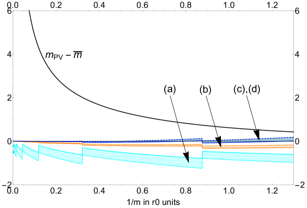
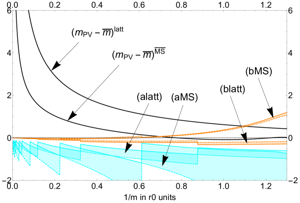
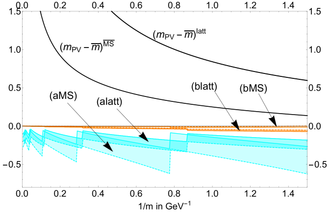
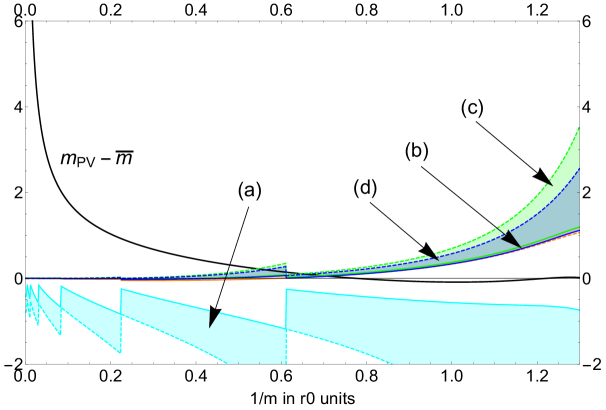
We also explore the scheme dependence by performing the computation in the lattice and the MS¯¯MS\overline{\rm MS} scheme. We will do these analyses for the cases with nf=0subscript𝑛𝑓0n_{f}=0 and nf=3subscript𝑛𝑓3n_{f}=3. The first in view of comparing with quenched lattice simulations, the second to simulate a more physical scenario, for which we can draw some conclusions that could be applied beyond the large-β0subscript𝛽0\beta_{0} limit. In Figs. 1, 2, and 3 we plot mPVm¯subscript𝑚PV¯𝑚m_{\rm PV}-{\overline{m}}, mPVmPsubscript𝑚PVsubscript𝑚𝑃m_{\rm PV}-m_{P}, mPVmPm¯Ωmsubscript𝑚PVsubscript𝑚𝑃¯𝑚subscriptΩ𝑚m_{\rm PV}-m_{P}-{\overline{m}}\Omega_{m}, mPVmPm¯Ωmn=NP+12NP(rnrn(as))αn+1subscript𝑚PVsubscript𝑚𝑃¯𝑚subscriptΩ𝑚superscriptsubscript𝑛subscript𝑁𝑃12subscript𝑁𝑃subscript𝑟𝑛superscriptsubscript𝑟𝑛assuperscript𝛼𝑛1m_{\rm PV}-m_{P}-{\overline{m}}\Omega_{m}-\sum_{n=N_{P}+1}^{2N_{P}}(r_{n}-r_{n}^{(\rm as)})\alpha^{n+1}, and mPVmPm¯Ωmn=NP+12NP(rnrn(as))αn+1m¯Ω2subscript𝑚PVsubscript𝑚𝑃¯𝑚subscriptΩ𝑚superscriptsubscript𝑛subscript𝑁𝑃12subscript𝑁𝑃subscript𝑟𝑛superscriptsubscript𝑟𝑛assuperscript𝛼𝑛1¯𝑚subscriptΩ2m_{\rm PV}-m_{P}-{\overline{m}}\Omega_{m}-\sum_{n=N_{P}+1}^{2N_{P}}(r_{n}-r_{n}^{(\rm as)})\alpha^{n+1}-{\overline{m}}\Omega_{-2} with nf=0subscript𝑛𝑓0n_{f}=0 light flavours. In the counting of Eq. (II.1) this corresponds to (0,0), (0,NPsubscript𝑁𝑃N_{P}), (1,0), (1,NPsubscript𝑁𝑃N_{P}), (2,0) precision. We do such computation in the lattice (Fig. 1) and the MS¯¯MS\overline{\rm MS} (Fig. 2) scheme. In Fig. 3 we compare the results in the lattice and MS¯¯MS\overline{\rm MS} scheme. We observe a very nice convergent pattern in all cases down to surprisingly small scales. To visualize the dependence on c𝑐c, we show the band generated by the smallest positive and negative possible values of c𝑐c that yield integer values for NPsubscript𝑁𝑃N_{P}. The size of the band generated by the different values of c𝑐c (the c𝑐c dependence) decreases after introducing ΩmsubscriptΩ𝑚\Omega_{m} to its associated sum. On the other hand Ω2subscriptΩ2\Omega_{-2} (an ultraviolet renormalon) gives a very small contribution, in particular in the lattice scheme. This is consistent with interpreting the lattice scheme as the MS¯¯MS\overline{\rm MS} scheme using a much higher renormalization scale μ𝜇\mu for the scale of the strong coupling.
Refer to caption

r01superscriptsubscript𝑟01r_{0}^{-1}

Refer to caption

r01superscriptsubscript𝑟01r_{0}^{-1}

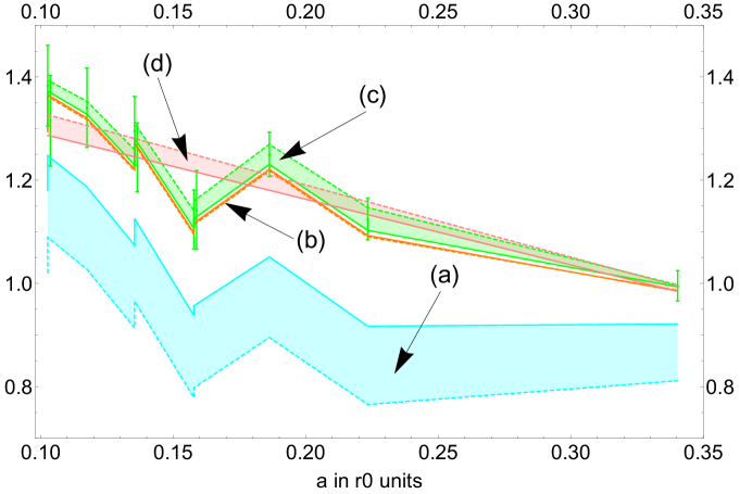
Figure 1: Upper panel: We plot mPVm¯subscript𝑚PV¯𝑚m_{\rm PV}-{\overline{m}} (black line) and the differences: (a) mPVmPsubscript𝑚PVsubscript𝑚𝑃m_{\rm PV}-m_{P} (cyan), (b) mPVmPm¯Ωmsubscript𝑚PVsubscript𝑚𝑃¯𝑚subscriptΩ𝑚m_{\rm PV}-m_{P}-{\overline{m}}\Omega_{m} (orange), (c) mPVmPm¯Ωmn=NP+12NP(rnrn(as))αn+1subscript𝑚PVsubscript𝑚𝑃¯𝑚subscriptΩ𝑚superscriptsubscript𝑛subscript𝑁𝑃12subscript𝑁𝑃subscript𝑟𝑛superscriptsubscript𝑟𝑛assuperscript𝛼𝑛1m_{\rm PV}-m_{P}-{\overline{m}}\Omega_{m}-\sum_{n=N_{P}+1}^{2N_{P}}(r_{n}-r_{n}^{(\rm as)})\alpha^{n+1} (green), and (d) mPVmPm¯Ωmn=NP+12NP(rnrn(as))αn+1m¯Ω2subscript𝑚PVsubscript𝑚𝑃¯𝑚subscriptΩ𝑚superscriptsubscript𝑛subscript𝑁𝑃12subscript𝑁𝑃subscript𝑟𝑛superscriptsubscript𝑟𝑛assuperscript𝛼𝑛1¯𝑚subscriptΩ2m_{\rm PV}-m_{P}-{\overline{m}}\Omega_{m}-\sum_{n=N_{P}+1}^{2N_{P}}(r_{n}-r_{n}^{(\rm as)})\alpha^{n+1}-{\overline{m}}\Omega_{-2} (blue) in the large β0subscript𝛽0\beta_{0} approximation using the lattice scheme with nf=0subscript𝑛𝑓0n_{f}=0 light flavours. For each difference, the bands are generated by the difference of the prediction produced by the smallest positive or negative possible values of c𝑐c that yields integer values for NPsubscript𝑁𝑃N_{P}. The (c) and (d) bands are one on top of the other. Lower panel: As in the upper panel but in a smaller range. r01400superscriptsubscript𝑟01400r_{0}^{-1}\approx 400 MeV. The value of NPsubscript𝑁𝑃N_{P} depends on the scale 1/m1𝑚1/m we use. For instance for c𝑐c positive, NP=9subscript𝑁𝑃9N_{P}=9 for 1/m[0.003,0.0045]1𝑚0.0030.00451/m\in[0.003,0.0045], NP=8subscript𝑁𝑃8N_{P}=8 for 1/m[0.006,0.0015]1𝑚0.0060.00151/m\in[0.006,0.0015], NP=7subscript𝑁𝑃7N_{P}=7 for 1/m[0.0165,0.0435]1𝑚0.01650.04351/m\in[0.0165,0.0435], NP=6subscript𝑁𝑃6N_{P}=6 for 1/m[0.045,0.01185]1𝑚0.0450.011851/m\in[0.045,0.01185], NP=5subscript𝑁𝑃5N_{P}=5 for 1/m[0.12,0.321]1𝑚0.120.3211/m\in[0.12,0.321], NP=4subscript𝑁𝑃4N_{P}=4 for 1/m[0.3225,0.876]1𝑚0.32250.8761/m\in[0.3225,0.876] and NP=3subscript𝑁𝑃3N_{P}=3 for 1/m[0.8775,1.299]1𝑚0.87751.2991/m\in[0.8775,1.299].
Refer to caption

r01superscriptsubscript𝑟01r_{0}^{-1}

Refer to caption

r01superscriptsubscript𝑟01r_{0}^{-1}

Figure 2: As in Fig. 1 but in the MS¯¯MS\overline{\rm MS} scheme. The values of NPsubscript𝑁𝑃N_{P} for c𝑐c positive are, for instance, NP=6subscript𝑁𝑃6N_{P}=6 for 1/m=0.0031𝑚0.0031/m=0.003, NP=5subscript𝑁𝑃5N_{P}=5 for 1/m[0.0045,0.0105]1𝑚0.00450.01051/m\in[0.0045,0.0105], NP=4subscript𝑁𝑃4N_{P}=4 for 1/m[0.012,0.03]1𝑚0.0120.031/m\in[0.012,0.03], NP=3subscript𝑁𝑃3N_{P}=3 for 1/m[0.0315,0.0825]1𝑚0.03150.08251/m\in[0.0315,0.0825], NP=2subscript𝑁𝑃2N_{P}=2 for 1/m[0.084,0.2235]1𝑚0.0840.22351/m\in[0.084,0.2235], NP=1subscript𝑁𝑃1N_{P}=1 for 1/m[0.225,0.6105]1𝑚0.2250.61051/m\in[0.225,0.6105] and NP=0subscript𝑁𝑃0N_{P}=0 for 1/m[0.612,1.5]1𝑚0.6121.51/m\in[0.612,1.5].
Refer to caption

r01superscriptsubscript𝑟01r_{0}^{-1}

Refer to caption

r01superscriptsubscript𝑟01r_{0}^{-1}

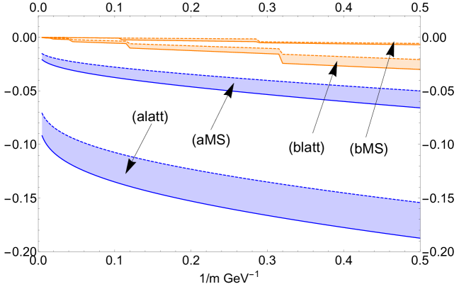
Figure 3: Comparison of lattice and MS¯¯MS\overline{\rm MS} scheme results for nf=0subscript𝑛𝑓0n_{f}=0 obtained in Figs. 1 and 2. Upper panel: We plot mPVm¯subscript𝑚PV¯𝑚m_{\rm PV}-{\overline{m}} and the differences: (a) mPVmPsubscript𝑚PVsubscript𝑚𝑃m_{\rm PV}-m_{P}, and (b) mPVmPm¯Ωmsubscript𝑚PVsubscript𝑚𝑃¯𝑚subscriptΩ𝑚m_{\rm PV}-m_{P}-{\overline{m}}\Omega_{m} in the lattice and MS¯¯MS\overline{\rm MS} scheme with nf=0subscript𝑛𝑓0n_{f}=0 light flavours. Lower panel: Lower panel Figs. 1 and 2 combined.

Let us discuss the results in more detail. We first observe that the m¯¯𝑚{\overline{m}} dependence of mPVsubscript𝑚PVm_{\rm PV} is basically eliminated in mPVmPsubscript𝑚PVsubscript𝑚𝑃m_{\rm PV}-m_{P}, as expected. This happens both in the lattice and MS¯¯MS\overline{\rm MS} scheme. The latter shows a stronger c𝑐c dependence. This is to be expected, as in the MS¯¯MS\overline{\rm MS}, we truncate at smaller orders in N𝑁N. This makes the truncation error bigger. As we can see in the upper panel of Fig. 3, both schemes yield consistent predictions for mPVmPsubscript𝑚PVsubscript𝑚𝑃m_{\rm PV}-m_{P}. We can draw some interesting observations out of this analysis. For mPVmPsubscript𝑚PVsubscript𝑚𝑃m_{\rm PV}-m_{P} is better to choose a larger factorization scale, if we have enough coefficients of the perturbative expansion. This is particularly so at large distances: We can still get good results at very large distances in the lattice scheme.

We now turn to mPVmPm¯Ωmsubscript𝑚PVsubscript𝑚𝑃¯𝑚subscriptΩ𝑚m_{\rm PV}-m_{P}-{\overline{m}}\Omega_{m}. Adding the new correction brings much better agreement with expectations (which we remind is to get zero). After the introduction of m¯Ωm¯𝑚subscriptΩ𝑚{\overline{m}}\Omega_{m}, the MS¯¯MS\overline{\rm MS} scheme yields more accurate results than the lattice scheme. This can already be seen in the upper panel of Fig. 3, and in greater detail in the lower panel of Fig. 3.

mPVmPm¯Ωmsubscript𝑚PVsubscript𝑚𝑃¯𝑚subscriptΩ𝑚m_{\rm PV}-m_{P}-{\overline{m}}\Omega_{m} shows some dependence on m¯¯𝑚{\overline{m}}, which is more pronounced in the lattice than in the MS¯¯MS\overline{\rm MS} scheme. As in the large β0subscript𝛽0\beta_{0} approximation the difference between both schemes is somewhat equivalent to a change of scale, these results point to that μ=m¯𝜇¯𝑚\mu={\overline{m}} in MS¯¯MS\overline{\rm MS} scheme is close to the natural scale and minimize higher order corrections. Note that the lattice scheme computation is equivalent to the MS¯¯MS\overline{\rm MS} scheme choosing μlatt=μMS¯eclatt2ecMS¯2subscript𝜇𝑙𝑎𝑡𝑡subscript𝜇¯MSsuperscript𝑒subscript𝑐𝑙𝑎𝑡𝑡2superscript𝑒subscript𝑐¯MS2\mu_{latt}=\mu_{\overline{\rm MS}}e^{\frac{-c_{latt}}{2}}e^{\frac{c_{\overline{\rm MS}}}{2}}. This gives around a factor 30 (!). Once n=NP+12NP(rnrn(as))αn+1superscriptsubscript𝑛subscript𝑁𝑃12subscript𝑁𝑃subscript𝑟𝑛superscriptsubscript𝑟𝑛assuperscript𝛼𝑛1\sum_{n=N_{P}+1}^{2N_{P}}(r_{n}-r_{n}^{(\rm as)})\alpha^{n+1} is incorporated in the prediction most of the difference between schemes disappears. The effect of introducing Ω2subscriptΩ2\Omega_{-2} is very small, in particular in the lattice scheme. This is to be expected, since the lattice scheme corresponds to a larger renormalization scale μ𝜇\mu. In any case, the difference between schemes gets smaller and smaller as we go to higher orders in the hyperasymptotic expansion, in particular at short distances. We also want to stress that this analysis opens the window to apply perturbation theory at rather large distances. Note that in the upper panel plots in Figs. 1, 2, and 3, we have gone to very large distances.

As some concluding remarks let us emphasize the following points. mPVmPsubscript𝑚PVsubscript𝑚𝑃m_{\rm PV}-m_{P} is more or less constant with relatively large uncertainties. This is to be expected, as the next correction in magnitude is m¯Ωm¯𝑚subscriptΩ𝑚{\overline{m}}\Omega_{m} which is approximately constant (mildly modulated by α(μ)𝛼𝜇\sqrt{\alpha(\mu)}). After introducing this term the error is much smaller and we can see more structure. In particular we are sensitive to n=NP+12NP(rnrn(as))αn+1superscriptsubscript𝑛subscript𝑁𝑃12subscript𝑁𝑃subscript𝑟𝑛superscriptsubscript𝑟𝑛assuperscript𝛼𝑛1\sum_{n=N_{P}+1}^{2N_{P}}(r_{n}-r_{n}^{(\rm as)})\alpha^{n+1}. Here we find (at the level of precision we have now) a sizable difference between lattice and MS¯¯MS\overline{\rm MS}. This can be expected: n=NP+12NP(rnrn(as))αn+1superscriptsubscript𝑛subscript𝑁𝑃12subscript𝑁𝑃subscript𝑟𝑛superscriptsubscript𝑟𝑛assuperscript𝛼𝑛1\sum_{n=N_{P}+1}^{2N_{P}}(r_{n}-r_{n}^{(\rm as)})\alpha^{n+1} is the object we expect to be more sensitive to the scale.

Another interesting observation is that truncated sums behave better in the lattice scheme than in the MS¯¯MS\overline{\rm MS} scheme. Nevertheless, this could be misleading. The sums are truncated at the minimal term. Therefore, one needs more terms in the lattice scheme. If the number of terms is not an issue (which could be the case with dedicated numerical stochastic perturbation theory (NSPT) DiRenzo:1994sy ; DiRenzo:2004hhl computations in the lattice scheme) then the lattice scheme looks better. But as soon as ΩmsubscriptΩ𝑚\Omega_{m} is introduced in the computation MS¯¯MS\overline{\rm MS} behaves better (at least in the large β0subscript𝛽0\beta_{0} approximation).

Overall, we observe a very nice convergence pattern up to (surprisingly) rather large scales in the lattice and MS¯¯MS\overline{\rm MS} scheme. The agreement with the theoretical prediction (which is zero) is perfect at short distances. The estimated error is also expected to be small. It will be interesting to see if this also happens beyond the large β0subscript𝛽0\beta_{0}.

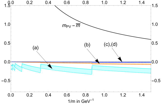
We now turn to the nf=3subscript𝑛𝑓3n_{f}=3 case. To easy the comparison with HyperI , we use the same value: ΛMS¯(nf=3)=174subscriptΛ¯MSsubscript𝑛𝑓3174\Lambda_{\overline{\rm MS}}(n_{f}=3)=174 MeV (which yields α(Mτ)0.3𝛼subscript𝑀𝜏0.3\alpha(M_{\tau})\approx 0.3). The general conclusions do not change if we fix ΛMS¯subscriptΛ¯MS\Lambda_{\overline{\rm MS}} (in the large β0subscript𝛽0\beta_{0} approximation) using the world average value of α𝛼\alpha. We note that ΛQCDsubscriptΛQCD\Lambda_{\rm QCD} for the physical case (nf=3subscript𝑛𝑓3n_{f}=3) is smaller than for the nf=0subscript𝑛𝑓0n_{f}=0 case (if one sets the physical scale according to r01400superscriptsubscript𝑟01400r_{0}^{-1}\approx 400 MeV). On top of that the running is less important. All this points to that the convergence should be even better than in the nf=0subscript𝑛𝑓0n_{f}=0 case (and it was quite good already there). We show our results in Figs. 4, 5 and 6 (these are the analogous of Figs. 1, 2 and 3 but with nf=3subscript𝑛𝑓3n_{f}=3). These plots confirm our expectations. Down to scales as low as 667 MeV we see no sign of breakdown of the OPE. This is so in both the lattice and the MS¯¯MS\overline{\rm MS} schemes. Note that the precision we get is extremely high as we go to small scales: Using truncation (c): mP+m¯Ωm+n=NP+12NP(rnrn(as))αn+1subscript𝑚𝑃¯𝑚subscriptΩ𝑚superscriptsubscript𝑛subscript𝑁𝑃12subscript𝑁𝑃subscript𝑟𝑛superscriptsubscript𝑟𝑛assuperscript𝛼𝑛1m_{P}+{\overline{m}}\Omega_{m}+\sum_{n=N_{P}+1}^{2N_{P}}(r_{n}-r_{n}^{(\rm as)})\alpha^{n+1}, one gets mPVsubscript𝑚PVm_{\rm PV} in the MS¯¯MS\overline{\rm MS} scheme with a precision below 1 MeV at scales of the order of the mass of the bottom, and in the lattice scheme with a precision below 2 MeV. Using truncation (d): mP+m¯Ωm+n=NP+12NP(rnrn(as))αn+1+m¯Ω2subscript𝑚𝑃¯𝑚subscriptΩ𝑚superscriptsubscript𝑛subscript𝑁𝑃12subscript𝑁𝑃subscript𝑟𝑛superscriptsubscript𝑟𝑛assuperscript𝛼𝑛1¯𝑚subscriptΩ2m_{P}+{\overline{m}}\Omega_{m}+\sum_{n=N_{P}+1}^{2N_{P}}(r_{n}-r_{n}^{(\rm as)})\alpha^{n+1}+{\overline{m}}\Omega_{-2}, the precision does not significantly change, in particular in the lattice scheme. This reflects that ultraviolet renormalons play a minor role. The rest of the discussion follows parallel the one for nf=0subscript𝑛𝑓0n_{f}=0.

Refer to caption

GeV

Refer to caption

GeV

Figure 4: As in Fig. 1 but with nf=3subscript𝑛𝑓3n_{f}=3 light flavours. The value of NPsubscript𝑁𝑃N_{P} depends on the scale 1/m1𝑚1/m we use. For instance for c𝑐c positive, NP=1subscript𝑁𝑃1N_{P}=1 for 1/m=0.0051𝑚0.0051/m=0.005, NP=10subscript𝑁𝑃10N_{P}=10 for 1/m[0.01,0.015]1𝑚0.010.0151/m\in[0.01,0.015], NP=9subscript𝑁𝑃9N_{P}=9 for 1/m[0.02,0.04]1𝑚0.020.041/m\in[0.02,0.04], NP=8subscript𝑁𝑃8N_{P}=8 for 1/m[0.045,0.115]1𝑚0.0450.1151/m\in[0.045,0.115], NP=7subscript𝑁𝑃7N_{P}=7 for 1/m[0.12,0.315]1𝑚0.120.3151/m\in[0.12,0.315], NP=6subscript𝑁𝑃6N_{P}=6 for 1/m[0.32,0.865]1𝑚0.320.8651/m\in[0.32,0.865], and NP=5subscript𝑁𝑃5N_{P}=5 for 1/m[0.87,1.5]1𝑚0.871.51/m\in[0.87,1.5].
Refer to caption

GeV

Refer to caption

GeV

Figure 5: As in Fig. 1 but with nf=3subscript𝑛𝑓3n_{f}=3 light flavours and in the MS¯¯MS\overline{\rm MS} scheme. The value of NPsubscript𝑁𝑃N_{P} depends on the scale 1/m1𝑚1/m we use. For instance for c𝑐c positive, NP=7subscript𝑁𝑃7N_{P}=7 for 1/m=0.0051𝑚0.0051/m=0.005, NP=6subscript𝑁𝑃6N_{P}=6 for 1/m=0.011𝑚0.011/m=0.01, NP=5subscript𝑁𝑃5N_{P}=5 for 1/m[0.015,0.035]1𝑚0.0150.0351/m\in[0.015,0.035], NP=4subscript𝑁𝑃4N_{P}=4 for 1/m[0.04,0.105]1𝑚0.040.1051/m\in[0.04,0.105], NP=3subscript𝑁𝑃3N_{P}=3 for 1/m[0.11,0.285]1𝑚0.110.2851/m\in[0.11,0.285], NP=2subscript𝑁𝑃2N_{P}=2 for 1/m[0.29,0.775]1𝑚0.290.7751/m\in[0.29,0.775], and NP=1subscript𝑁𝑃1N_{P}=1 for 1/m[0.78,1.5]1𝑚0.781.51/m\in[0.78,1.5].
Refer to caption

GeV

Refer to caption

GeV

Figure 6: Comparison of lattice and MS¯¯MS\overline{\rm MS} scheme results for nf=3subscript𝑛𝑓3n_{f}=3. Upper panel: We plot mPVsubscript𝑚PVm_{\rm PV} and the differences: (a) mPVmPsubscript𝑚PVsubscript𝑚𝑃m_{\rm PV}-m_{P}, and (b) mPVmPm¯Ωmsubscript𝑚PVsubscript𝑚𝑃¯𝑚subscriptΩ𝑚m_{\rm PV}-m_{P}-{\overline{m}}\Omega_{m} in the lattice and MS¯¯MS\overline{\rm MS} scheme with nf=3subscript𝑛𝑓3n_{f}=3 light flavours. Lower panel: Fig. 4 and Fig. 5 combined.

In the above numerics, we have used the exact expression for ΩmsubscriptΩ𝑚\Omega_{m} and Ω2subscriptΩ2\Omega_{-2}. In full QCD, we will not know the exact expression. Therefore, it makes sense to study how well the exact result is reproduced by its semiclassical expansion. We observed in HyperI that ΩmsubscriptΩ𝑚\Omega_{m} is very well saturated by the first terms of such expansion. Truncating the expansion produces differences much smaller than the typical precision of the different terms of the hyperasymptotic expansion. For Ω2subscriptΩ2\Omega_{-2}, we compare in Table 1 and 2 the exact result and the truncated semiclassical expansion for an illustrative set of values. We observe that the exact result is very well saturated by the first terms of the expansion computed in Eq. (38). Truncating the expansion produces differences much smaller than the typical precision of the different terms of the hyperasymptotic expansion. As expected nf=3subscript𝑛𝑓3n_{f}=3 is better than nf=0subscript𝑛𝑓0n_{f}=0. Note that in the large β0subscript𝛽0\beta_{0} approximation we exactly have Λ=μe2π/(β0α(μ))Λ𝜇superscript𝑒2𝜋subscript𝛽0𝛼𝜇\Lambda=\mu e^{-2\pi/(\beta_{0}\alpha(\mu))}.

MS¯¯MS\overline{\text{MS}}-Scheme (nf=0subscript𝑛𝑓0n_{f}=0)
m¯¯𝑚{\overline{m}} in r01superscriptsubscript𝑟01r_{0}^{-1} c𝑐c m¯Ω¯𝑚Ω{\overline{m}}\OmegaExact |ΩLOΩExact1|×102ΩLOΩExact1superscript102\left|\frac{\Omega\text{LO}}{\Omega\text{Exact}}-1\right|\times 10^{2} |ΩNLOΩExact1|×103ΩNLOΩExact1superscript103\left|\frac{\Omega\text{NLO}}{\Omega\text{Exact}}-1\right|\times 10^{3} |ΩNNLOΩExact1|×104ΩNNLOΩExact1superscript104\left|\frac{\Omega\text{NNLO}}{\Omega\text{Exact}}-1\right|\times 10^{4}
0.6667 0.1786 0.2089 33.8725 147.64 3372.63
0.8333 0.5693 0.0572 8.1940 93.6387 922.993
1 0.8885 0.0362 14.1752 45.6019 16.0275
1.25 1.2791 0.0260 5.7282 13.6703 130.93
1.6667 0.0321 0.0199 12.0969 7.3723 12.2818
2.5 0.7419 0.0094 4.9357 7.7804 6.5465
5 0.2047 0.0042 2.9590 0.5254 4.8485
10 1.4182 0.0018 0.2254 2.2970 2.3334
100 0.1972 0.0001 1.2994 0.1190 0.3921
Lattice-Scheme (nf=0subscript𝑛𝑓0n_{f}=0)
m¯¯𝑚{\overline{m}} in r01superscriptsubscript𝑟01r_{0}^{-1} c𝑐c m¯Ω¯𝑚Ω{\overline{m}}\OmegaExact×109absentsuperscript109\times 10^{9} |ΩLOΩExact1|×103ΩLOΩExact1superscript103\left|\frac{\Omega\text{LO}}{\Omega\text{Exact}}-1\right|\times 10^{3} |ΩNLOΩExact1|×104ΩNLOΩExact1superscript104\left|\frac{\Omega\text{NLO}}{\Omega\text{Exact}}-1\right|\times 10^{4} |ΩNNLOΩExact1|×105ΩNNLOΩExact1superscript105\left|\frac{\Omega\text{NNLO}}{\Omega\text{Exact}}-1\right|\times 10^{5}
0.6667 0.8101 0.33643 23.0068 12.0234 0.06620
0.8333 1.2008 0.26320 13.94 5.2020 12.6513
1 1.5200 0.21971 11.9588 13.8372 5.6692
1.25 0.1599 0.17233 20.0735 0.3374 6.8322
1.6667 0.6636 0.12061 15.0134 9.1010 3.3885
2.5 1.3734 7.7980 1.2511 7.4891 5.2999
5 0.8362 3.5950 14.9013 4.4610 0.4998
10 0.2990 1.7262 4.2813 2.3906 2.5543
100 0.8287 14.527 9.6569 1.8830 0.05590
Table 1: m¯Ω2¯𝑚subscriptΩ2{\overline{m}}\Omega_{-2} in the large β0subscript𝛽0\beta_{0} approximation for nf=0subscript𝑛𝑓0n_{f}=0 in r01superscriptsubscript𝑟01r_{0}^{-1} units compared with Eq. (38) truncated at different powers of α𝛼\alpha. Upper panel computed in the MS¯¯MS\overline{\rm MS} scheme. Lower panel in the lattice scheme. Lattice seems to be better but both schemes yield very good results.
MS¯¯MS\overline{\text{MS}}-Scheme (nf=3subscript𝑛𝑓3n_{f}=3)
m¯¯𝑚{\overline{m}} in GeV c𝑐c m¯Ω¯𝑚Ω{\overline{m}}\OmegaExact |ΩLOΩExact1|×102ΩLOΩExact1superscript102\left|\frac{\Omega\text{LO}}{\Omega\text{Exact}}-1\right|\times 10^{2} |ΩNLOΩExact1|×103ΩNLOΩExact1superscript103\left|\frac{\Omega\text{NLO}}{\Omega\text{Exact}}-1\right|\times 10^{3} |ΩNNLOΩExact1|×104ΩNNLOΩExact1superscript104\left|\frac{\Omega\text{NNLO}}{\Omega\text{Exact}}-1\right|\times 10^{4}
0.6667 0.4916 0.00375 3.6513 8.8280 16.5412
0.8333 0.8113 0.00274 5.0007 2.9016 7.864
1 1.0724 0.00223 1.6450 3.9632 11.1774
1.25 1.3921 0.00183 6.2621 3.6008 0.7661
1.6667 0.3717 0.00119 0.8631 2.7541 4.6880
2.5 0.9525 0.00072 2.2110 0.5893 3.1281
5 0.5130 0.00032 1.7608 1.5455 0.9363
10 0.0735 0.00015 2.8072 0.2396 0.5520
100 0.5069 0.00001 0.9405 0.4412 0.1384
Lattice-Scheme (nf=3subscript𝑛𝑓3n_{f}=3)
m¯¯𝑚{\overline{m}} in GeV c𝑐c m¯Ω¯𝑚Ω{\overline{m}}\OmegaExact×1011absentsuperscript1011\times 10^{11} |ΩLOΩExact1|×103ΩLOΩExact1superscript103\left|\frac{\Omega\text{LO}}{\Omega\text{Exact}}-1\right|\times 10^{3} |ΩNLOΩExact1|×104ΩNLOΩExact1superscript104\left|\frac{\Omega\text{NLO}}{\Omega\text{Exact}}-1\right|\times 10^{4} |ΩNNLOΩExact1|×105ΩNNLOΩExact1superscript105\left|\frac{\Omega\text{NNLO}}{\Omega\text{Exact}}-1\right|\times 10^{5}
0.6667 0.6457 0.13921 14.5539 5.0568 0.1286
0.8333 0.9653 0.10969 9.6413 1.9386 3.4992
1 1.2264 9.1458 6.7772 6.1070 1.8276
1.25 0.1137 7.2422 15.151 0.1208 2.0634
1.6667 0.5258 5.1755 9.9772 4.3766 1.2143
2.5 1.1065 3.3731 1.7019 3.6030 1.9541
5 0.6670 1.5918 10.8713 2.5255 0.06625
10 0.2275 77.282 4.1604 1.2278 1.1874
100 0.6609 674.45 7.7077 1.7587 4.5364
Table 2: m¯Ω2¯𝑚subscriptΩ2{\overline{m}}\Omega_{-2} in the large β0subscript𝛽0\beta_{0} approximation for nf=3subscript𝑛𝑓3n_{f}=3 in GeV units compared with Eq. (38) truncated at different powers of α𝛼\alpha. Upper panel computed in the MS¯¯MS\overline{\rm MS} scheme. Lower panel in the lattice scheme. Lattice seems to be better but both schemes yield very good results.

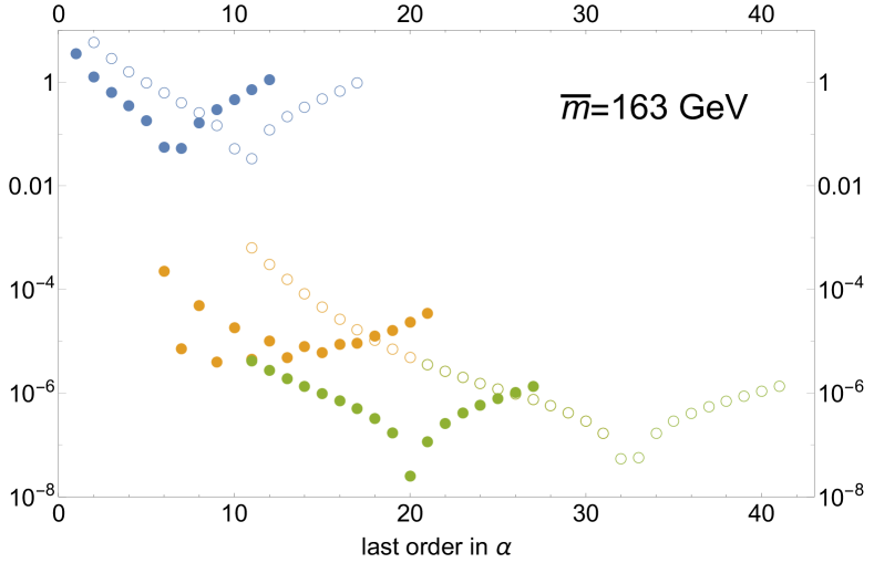
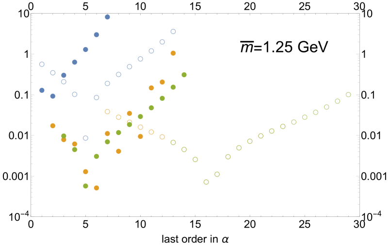
An alternative, very effective, presentation of the above results can be done by plotting the relative accuracy of the prediction at each order in α𝛼\alpha, and at each order of the superasymptotic expansion. We note that we have one observable for each value of m¯¯𝑚{\overline{m}}. Therefore, for illustration, we take two extreme cases. We use mPVsubscript𝑚PVm_{\rm PV} with m¯=1.25¯𝑚1.25{\overline{m}}=1.25 GeV and m¯=163¯𝑚163{\overline{m}}=163 GeV. For the theoretical prediction we take the smallest positive value of c𝑐c corresponding to lattice or MS¯¯MS\overline{\rm MS} scheme.333Taking different values of c𝑐c do not change the picture. The new points stand on top of the old ones where they overlap. We use the exact expressions for ΩmsubscriptΩ𝑚\Omega_{m} and Ω2subscriptΩ2\Omega_{-2}. Nevertheless, the NNLO truncated expression for ΩmsubscriptΩ𝑚\Omega_{m} is precise enough to yield the same result. For Ω2subscriptΩ2\Omega_{-2} we could truncate earlier with no visible effect. We show the results in Fig. 7. We stress that several terms of the hyperasymptotic expansion are included. First, we nicely see that, once reached the minimum, NNPsimilar-to𝑁subscript𝑁𝑃N\sim N_{P}, both schemes yield similar precision, but in the lattice scheme (bigger factorization scale μ𝜇\mu) more terms of the perturbative expansions are needed to reach the same precision. We can see a gap when ΩmsubscriptΩ𝑚\Omega_{m} is included, with significant better precision in the MS¯¯MS\overline{\rm MS} scheme. One important lesson one may extrapolate from this exercise is that, if the number of perturbative coefficients is fixed, the smaller the renormalization scale μ𝜇\mu, the better. One can obtain much better precision for an equal number of perturbative coefficients. Another observation is that the minimal term determined numerically need not to coincide with the minimal term computed using N=NP𝑁subscript𝑁𝑃N=N_{P} (though it should not be much different). The difference reflects how much the exact coefficient is saturated by the asymptotic expression. The effect of Ω2subscriptΩ2\Omega_{-2} is very small compared with the effect due to ΩmsubscriptΩ𝑚\Omega_{m}. For the case of the top (m¯=163¯𝑚163{\overline{m}}=163 GeV) we can still see the sign alternating behavior of the perturbative series associated to the d=2𝑑2d=-2 renormalon in the MS¯¯MS\overline{\rm MS} scheme. In the lattice scheme the effect is so small that it cannot be seen and the precision is set by the next renormalon located at d=3𝑑3d=3. If one makes m¯¯𝑚{\overline{m}} small, m¯=1.25¯𝑚1.25{\overline{m}}=1.25 GeV, green and orange points mix in the MS¯¯MS\overline{\rm MS} scheme. This effect is more pronounced in the lattice scheme, where one can continuously move from the orange to the green points. The effect of the ultraviolet renormalon is very small and the precision is set by the u=3/2𝑢32u=3/2 renormalon.

Refer to caption
Refer to caption
Figure 7: |mPVmPVHyperasymptotic|subscript𝑚PVsuperscriptsubscript𝑚PVHyperasymptotic|m_{\rm PV}-m_{\rm PV}^{\rm Hyperasymptotic}| for m¯=163¯𝑚163{\overline{m}}=163 GeV (upper panel) and m¯=1.25¯𝑚1.25{\overline{m}}=1.25 GeV (lower panel). Blue points are |mPVmN|subscript𝑚PVsubscript𝑚𝑁|m_{\rm PV}-m_{N}|. Orange points are |mPVmPm¯Ωmn=NP+1N(rnrn(as))αn+1|subscript𝑚PVsubscript𝑚𝑃¯𝑚subscriptΩ𝑚superscriptsubscript𝑛subscript𝑁𝑃1𝑁subscript𝑟𝑛superscriptsubscript𝑟𝑛assuperscript𝛼𝑛1|m_{\rm PV}-m_{P}-{\overline{m}}\Omega_{m}-\sum_{n=N_{P}+1}^{N}(r_{n}-r_{n}^{(\rm as)})\alpha^{n+1}| with c=1.21/1.39𝑐1.211.39c=1.21/1.39 and c=1.36/0.11𝑐1.360.11c=1.36/0.11 (the smallest positive values that yield integer NPsubscript𝑁𝑃N_{P}) in the MS¯¯MS\overline{\rm MS} and lattice scheme respectively for m¯=163/1.25¯𝑚1631.25{\overline{m}}=163/1.25 GeV. Green points are |mPVmPm¯Ωmn=NP+12NP(rnrn(as))αn+1m¯Ω2n=2NP+1N(rnrn(as))αn+1|subscript𝑚PVsubscript𝑚𝑃¯𝑚subscriptΩ𝑚superscriptsubscript𝑛subscript𝑁𝑃12subscript𝑁𝑃subscript𝑟𝑛superscriptsubscript𝑟𝑛assuperscript𝛼𝑛1¯𝑚subscriptΩ2superscriptsubscript𝑛2subscript𝑁𝑃1𝑁subscript𝑟𝑛superscriptsubscript𝑟𝑛assuperscript𝛼𝑛1|m_{\rm PV}-m_{P}-{\overline{m}}\Omega_{m}-\sum_{n=N_{P}+1}^{2N_{P}}(r_{n}-r_{n}^{(\rm as)})\alpha^{n+1}-{\overline{m}}\Omega_{-2}-\sum_{n=2N_{P}+1}^{N}(r_{n}-r_{n}^{(\rm as)})\alpha^{n+1}|, where in the last sum the two first renormalons are subtracted. Change of color correspond to the inclusion of ΩmsubscriptΩ𝑚\Omega_{m} and Ω2subscriptΩ2\Omega_{-2}. Full points have been computed in the MS¯¯MS\overline{\rm MS} scheme and empty points in the lattice scheme. We work with nf=3subscript𝑛𝑓3n_{f}=3.

III.2 (N,μ)𝑁𝜇(N,\mu)\rightarrow\infty. Eq. (4). Case 2)

We take Eq. (29) in the large β0subscript𝛽0\beta_{0} limit by setting b=0𝑏0b=0. As before, we have no analytic expressions to compare with (unlike the case of the static potential). Therefore, we directly focus on taking the limit 2B) and numerically check its convergence and how it compares with method 1).

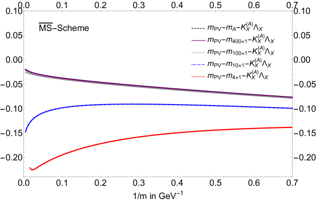
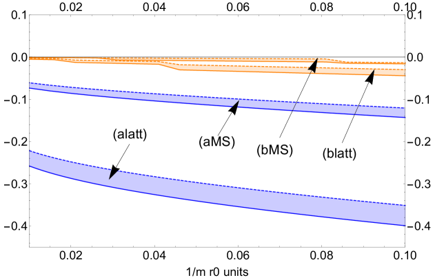
Method 2B) has the pleasant feature that the generated 𝒪(ΛQCD)𝒪subscriptΛQCD{\cal O}(\Lambda_{\rm QCD}) correction complies with the OPE. It also yields results that do not depend on N𝑁N (and μ𝜇\mu) anymore. Still, it has some errors and does not reach the precision of method 1). There is a residual scheme dependence associated to uncomputed terms of 𝒪(αΛQCD)𝒪𝛼subscriptΛQCD{\cal O}(\alpha\Lambda_{\rm QCD}). Part of it can be estimated by the residual dependence in csuperscript𝑐c^{\prime}. In order to estimate it, we compute mAsubscript𝑚𝐴m_{A} for different values of csuperscript𝑐c^{\prime}. On the one hand csuperscript𝑐c^{\prime} cannot be very large, as cα(m¯)superscript𝑐𝛼¯𝑚c^{\prime}\alpha({\overline{m}}) should be relatively close to zero. On the other hand we cannot make cα(m¯)superscript𝑐𝛼¯𝑚c^{\prime}\alpha({\overline{m}}) to get arbitrary close to zero, as the 𝒪(ΛQCD)𝒪subscriptΛQCD{\cal O}(\Lambda_{\rm QCD}) correction diverges logarithmically in csuperscript𝑐c^{\prime}. We also note that there is a value of c=cminsuperscript𝑐subscriptsuperscript𝑐minc^{\prime}=c^{\prime}_{\rm min} that makes that KX(A)=0superscriptsubscript𝐾𝑋𝐴0K_{X}^{(A)}=0 so that the 𝒪(ΛQCD)𝒪subscriptΛQCD{\cal O}(\Lambda_{\rm QCD}) correction vanishes. Therefore, we compute mAsubscript𝑚𝐴m_{A} for different values of csuperscript𝑐c^{\prime}. For illustration we show some results in Fig. 8. We draw lines for mPVmAKX(A)ΛXsubscript𝑚PVsubscript𝑚𝐴superscriptsubscript𝐾𝑋𝐴subscriptΛ𝑋m_{\rm PV}-m_{A}-K_{X}^{(A)}\Lambda_{X} at c=1superscript𝑐1c^{\prime}=1 and c=cminsuperscript𝑐subscript𝑐minc^{\prime}=c_{\rm min} generating a band. We also explore the dependence on the scheme by comparing the results in the lattice and MS¯¯MS\overline{\rm MS} scheme. We stress again that, in the large β0subscript𝛽0\beta_{0} approximation, lattice and MS¯¯MS\overline{\rm MS} schemes basically correspond to a redefinition of μ𝜇\mu, but quite large indeed. On the other hand the final result is μ𝜇\mu independent. Nevertheless, the way the μ𝜇\mu\rightarrow\infty limit is taken is fixed by NAsubscript𝑁𝐴N_{A}, as defined in Eq. (4), which is dependent on μ𝜇\mu. This explains why different results are obtained.
Refer to caption
Refer to caption
Figure 8: Upper panel: We plot (a) mPVmAKX(A)ΛXsubscript𝑚PVsubscript𝑚𝐴superscriptsubscript𝐾𝑋𝐴subscriptΛ𝑋m_{\rm PV}-m_{A}-K_{X}^{(A)}\Lambda_{X} for nf=0subscript𝑛𝑓0n_{f}=0 in the lattice and MS¯¯MS\overline{\rm MS} scheme. For each case, we generate bands by computing mAsubscript𝑚𝐴m_{A} with c=1superscript𝑐1c^{\prime}=1 and c=cmin=0.652superscript𝑐subscriptsuperscript𝑐min0.652c^{\prime}=c^{\prime}_{\rm min}=0.652. We also compare with (b) mPVmPm¯Ωmsubscript𝑚𝑃𝑉subscript𝑚𝑃¯𝑚subscriptΩ𝑚m_{PV}-m_{P}-{\overline{m}}\Omega_{m} obtained with method 1) with the bands generated for Fig. 3. Lower panel: As the upper panel with nf=3subscript𝑛𝑓3n_{f}=3, cmin=0.534subscriptsuperscript𝑐min0.534c^{\prime}_{\rm min}=0.534 and taking the the bands obtained with method 1) for Fig. 6 for (b) mPVmPm¯Ωmsubscript𝑚PVsubscript𝑚𝑃¯𝑚subscriptΩ𝑚m_{\rm PV}-m_{P}-{\overline{m}}\Omega_{m} .
Refer to caption
Refer to caption
Figure 9: Upper panel: We plot mPVmAKX(A)ΛXsubscript𝑚PVsubscript𝑚𝐴superscriptsubscript𝐾𝑋𝐴subscriptΛ𝑋m_{\rm PV}-m_{A}-K_{X}^{(A)}\Lambda_{X} for nf=3subscript𝑛𝑓3n_{f}=3 in the lattice scheme with c=1𝑐1c=1 versus the truncated sums mPVn=0NArnαn+1(μ)KX(A)ΛXsubscript𝑚PVsuperscriptsubscript𝑛0subscript𝑁𝐴subscript𝑟𝑛superscript𝛼𝑛1𝜇superscriptsubscript𝐾𝑋𝐴subscriptΛ𝑋m_{\rm PV}-\sum_{n=0}^{N_{A}}r_{n}\alpha^{n+1}(\mu)-K_{X}^{(A)}\Lambda_{X}, where μ𝜇\mu is fixed using NAsubscript𝑁𝐴N_{A} defined in Eq. (4). Lower panel: As in the upper panel but in the MS¯¯MS\overline{\rm MS} scheme.

In Fig. 8, we also compare with results obtained using method 1), more specifically we compare with mPVmPm¯Ωmsubscript𝑚PVsubscript𝑚𝑃¯𝑚subscriptΩ𝑚m_{\rm PV}-m_{P}-{\overline{m}}\Omega_{m}, as they both have analogous power accuracy (though method 1) is parametrically more precise). For ΩmsubscriptΩ𝑚\Omega_{m} we take the exact expression but using its approximated expression does not change the discussion, as the difference is very small. What we see is that the MS¯¯MS\overline{\rm MS} scheme yields more precise predictions than the lattice scheme, and that method 1) yields considerable better results than method 2B).

Another issue specific of method 2B) is to determine how large we need to take N𝑁N (and consequently μ𝜇\mu) of the truncated sum such that it approximates well mAsubscript𝑚𝐴m_{A}. For illustrative purposes we show the convergence in Fig. 9 for nf=3subscript𝑛𝑓3n_{f}=3 in the lattice and MS¯¯MS\overline{\rm MS} scheme. We find that we have to go to relatively large values of μ𝜇\mu (and N𝑁N) to get it precise. This can be a problem if one wants to go beyond the large β0subscript𝛽0\beta_{0}. This problem would be less severe if one can use the asymptotic expression for the coefficients beyond certain n𝑛n. Nicely enough, we find that the use of asymptotic expression for the coefficients for n>N𝑛superscript𝑁n>N^{*} (3similar-toabsent3\sim 3 in the MS¯¯MS\overline{\rm MS} and similar-to\sim 8 in the lattice scheme) is very efficient and basically yields the same results as the exact result. Finally, we also remind that to approximate well mAsubscript𝑚𝐴m_{A} by the truncated sum is more costly for small values of csuperscript𝑐c^{\prime}.

IV Λ¯PVsubscript¯ΛPV\overline{\Lambda}_{\rm PV} from lattice and B𝐵B physics

We now abandon the large-β0subscript𝛽0\beta_{0} approximation. Our aim is to determine Λ¯PVsubscript¯ΛPV\bar{\Lambda}_{\rm PV}. We will determine it first in gluedynamics (nf=0subscript𝑛𝑓0n_{f}=0) in Sec. IV.2. To study the scheme dependence of the result it will be useful to estimate the higher order coefficients of the β𝛽\beta function in the Wilson action lattice scheme. We do so in the next section.

IV.1 β𝛽\beta-function coefficients in the Wilson action lattice scheme
β3subscript𝛽3\beta_{3} β4subscript𝛽4\beta_{4} β5subscript𝛽5\beta_{5} β6subscript𝛽6\beta_{6}
1.16(3)×1061.163superscript106-1.16(3)\times 10^{6} 1.35(10)×1081.3510superscript108-1.35(10)\times 10^{8} 1.44(28)×10101.4428superscript1010-1.44(28)\times 10^{10} 1.41(60)×10121.4160superscript1012-1.41(60)\times 10^{12}
Table 3: Estimates of the coefficients of the beta function for the bare coupling in the lattice scheme using renormalon dominance and ZmMS¯=0.62superscriptsubscript𝑍𝑚¯MS0.62Z_{m}^{\overline{\rm MS}}=0.62 Bali:2013qla . The error quoted in the table gives the difference with the values of the beta coefficients obtained if one uses instead ZmMS¯=0.6superscriptsubscript𝑍𝑚¯MS0.6Z_{m}^{\overline{\rm MS}}=0.6 Ayala:2014yxa (which yields more negative values), and it is only meant to illustrate the typical spread of values of the beta coefficients if one uses different values of ZmMS¯superscriptsubscript𝑍𝑚¯MSZ_{m}^{\overline{\rm MS}}.
Refer to caption
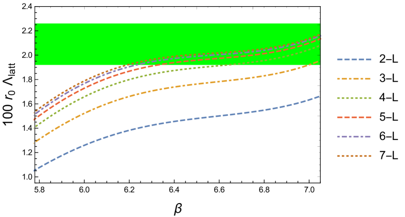
Figure 10: Same caption as in Fig. 1 of Bali:2014sja including more terms in the perturbative expansion using the β𝛽\beta-function coefficients listed in Table 3.

In Bali:2013pla ; Bali:2013qla it was shown that renormalon dominance allowed to give an accurate value for β3lattsuperscriptsubscript𝛽3𝑙𝑎𝑡𝑡\beta_{3}^{latt} assuming that c3subscript𝑐3c_{3} (see Eq. (44)) is already saturated by the renormalon in the MS¯¯MS\overline{\rm MS} scheme. We can estimate higher order terms of the β𝛽\beta function in the lattice scheme (using the Wilson action) by also assuming that for n>3𝑛3n>3 the coefficients cnsubscript𝑐𝑛c_{n} in the MS¯¯MS\overline{\rm MS} scheme are saturated by the renormalon. We show such estimates in Table 3. These coefficients of the β𝛽\beta function improve the agreement with the phenomenological parameterization of αlatt(1/a)subscript𝛼𝑙𝑎𝑡𝑡1𝑎\alpha_{latt}(1/a) obtained in Necco:2001xg in the range β(6,6.8)𝛽66.8\beta\in(6,6.8) (see Fig. 10). It is also worth mentioning that we observe a geometrical growth of the coefficients of the β𝛽\beta function. Elucubrative, this would indicate that the beta function in this scheme has a finite radius of convergence, and one can take the ansatz

βlatt(α)=νddνα2α{n=03βn(α4π)n+11.4×10⁸(α4π)511102α4π},superscript𝛽latt𝛼𝜈𝑑𝑑𝜈𝛼similar-to-or-equals2𝛼superscriptsubscript𝑛03subscript𝛽𝑛superscript𝛼4𝜋𝑛11.4superscript108superscript𝛼4𝜋511superscript102𝛼4𝜋\beta^{\rm latt}(\alpha)=\nu\frac{d}{d\nu}\alpha\simeq-2\alpha\left\{\sum_{n=0}^{3}\beta_{n}\left(\frac{\alpha}{4\pi}\right)^{n+1}-1.4\times 10^{8}\left(\frac{\alpha}{4\pi}\right)^{5}\frac{1}{1-10^{2}\frac{\alpha}{4\pi}}\right\}\,, (42)

which would have a pole at around β=6/g23.8𝛽6superscript𝑔2similar-to-or-equals3.8\beta=6/g^{2}\simeq 3.8.

IV.2 Λ¯PVsubscript¯ΛPV\bar{\Lambda}_{\rm PV} from lattice

Refer to caption
Refer to caption
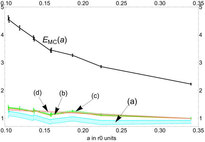
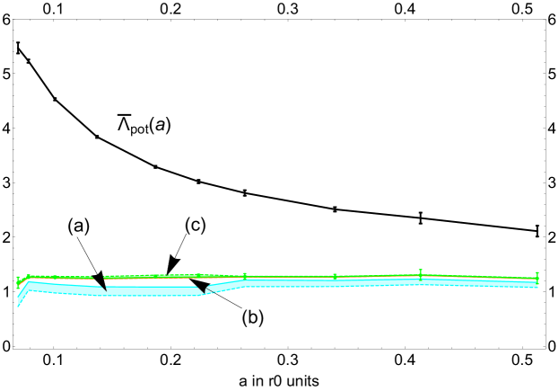
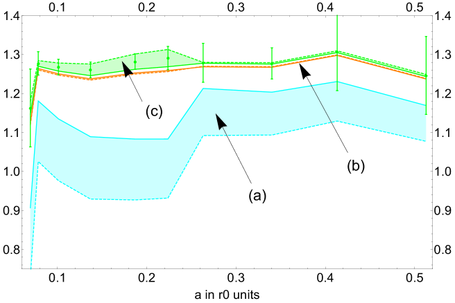
Figure 11: Upper panel: EMCsubscript𝐸MCE_{\rm MC} is the Montecarlo lattice data Duncan:1994uq ; Allton:1994tt ; Ewing:1995ih . The continuous lines are drawn to guide the eye. The other lines correspond to Eq. (45) truncated at different orders in the hyperasymptotic expansion. (a) EMC(a)δmP(1/a)subscript𝐸MC𝑎𝛿subscript𝑚𝑃1𝑎E_{\rm MC}(a)-\delta m_{P}(1/a), (b) EMC(a)δmP(1/a)1aΩmsubscript𝐸MC𝑎𝛿subscript𝑚𝑃1𝑎1𝑎subscriptΩ𝑚E_{\rm MC}(a)-\delta m_{P}(1/a)-\frac{1}{a}\Omega_{m}, (c) EMC(a)δmP(1/a)1aΩmNP+1N=2NP1a[cncn(as)]αn+1subscript𝐸MC𝑎𝛿subscript𝑚𝑃1𝑎1𝑎subscriptΩ𝑚superscriptsubscriptsubscript𝑁𝑃1superscript𝑁2subscript𝑁𝑃1𝑎delimited-[]subscript𝑐𝑛superscriptsubscript𝑐𝑛assuperscript𝛼𝑛1E_{\rm MC}(a)-\delta m_{P}(1/a)-\frac{1}{a}\Omega_{m}-\sum_{N_{P}+1}^{N^{\prime}=2N_{P}}\frac{1}{a}[c_{n}-c_{n}^{\rm(as)}]\alpha^{n+1} (in this last case we include the error of the lattice points in the middle of the band), (d) is the fit of the right-hand-side of Eq. (45) to Λ¯PV(nf=0)Kasubscript¯ΛPVsubscript𝑛𝑓0𝐾𝑎\bar{\Lambda}_{\rm PV}(n_{f}=0)-Ka. For each difference and for the final fit, the bands are generated by the difference of the prediction produced by the smallest positive or negative possible values of c𝑐c that yield integer values for NPsubscript𝑁𝑃N_{P}. Lower panel: As in the upper panel but in a smaller range. r01400superscriptsubscript𝑟01400r_{0}^{-1}\approx 400 MeV.

We determine Λ¯PVsubscript¯ΛPV\bar{\Lambda}_{\rm PV} in gluedynamics (nf=0subscript𝑛𝑓0n_{f}=0) from the energy of a meson made of a static quark and a light valence quark:

EMC(a)=δmlattPV+Λ¯PV+𝒪(aΛQCD2).subscript𝐸MC𝑎𝛿subscriptsuperscript𝑚PVlattsubscript¯ΛPV𝒪𝑎superscriptsubscriptΛQCD2E_{\rm MC}(a)=\delta m^{\rm PV}_{\rm latt}+\bar{\Lambda}_{\rm PV}+{\cal O}(a\Lambda_{\rm QCD}^{2})\,. (43)

δmlattPV𝛿subscriptsuperscript𝑚PVlatt\delta m^{\rm PV}_{\rm latt} has the following asymptotic series in powers of α=αlatt(1/a)𝛼subscript𝛼latt1𝑎\alpha=\alpha_{\rm latt}(1/a):

δmlattPVn=01acnαn+1,similar-to𝛿subscriptsuperscript𝑚PVlattsuperscriptsubscript𝑛01𝑎subscript𝑐𝑛superscript𝛼𝑛1\delta m^{\rm PV}_{\rm latt}\sim\sum_{n=0}^{\infty}\frac{1}{a}c_{n}\alpha^{n+1}\,, (44)

where rn(as)(ν)ν=cn(as)superscriptsubscript𝑟𝑛as𝜈𝜈superscriptsubscript𝑐𝑛as\frac{r_{n}^{\rm(as)}(\nu)}{\nu}=c_{n}^{\rm(as)}, since mPVsubscript𝑚PVm_{\rm PV} and δmlattPV𝛿subscriptsuperscript𝑚PVlatt\delta m^{\rm PV}_{\rm latt} have the same leading infared renormalon (located at d=1𝑑1d=1). The coefficients cnsubscript𝑐𝑛c_{n} are known from n=0÷19𝑛019n=0\div 19 in the lattice scheme for a Wilson action Bauer:2011ws ; Bali:2013pla ; Bali:2013qla . We then adapt Eq. (19) to δmlattPV𝛿subscriptsuperscript𝑚PVlatt\delta m^{\rm PV}_{\rm latt} to determine Λ¯PVsubscript¯ΛPV\bar{\Lambda}_{\rm PV}:

Λ¯PV(nf=0)=EMC(a)δmlattP1aΩmNP+1N=2NP1a[cncn(as)]αn+1+𝒪(aΛQCD2).subscript¯ΛPVsubscript𝑛𝑓0subscript𝐸MC𝑎𝛿subscriptsuperscript𝑚𝑃latt1𝑎subscriptΩ𝑚superscriptsubscriptsubscript𝑁𝑃1superscript𝑁2subscript𝑁𝑃1𝑎delimited-[]subscript𝑐𝑛superscriptsubscript𝑐𝑛assuperscript𝛼𝑛1𝒪𝑎superscriptsubscriptΛQCD2\bar{\Lambda}_{\rm PV}(n_{f}=0)=E_{\rm MC}(a)-\delta m^{P}_{\rm latt}-\frac{1}{a}\Omega_{m}-\sum_{N_{P}+1}^{N^{\prime}=2N_{P}}\frac{1}{a}[c_{n}-c_{n}^{\rm(as)}]\alpha^{n+1}+{\cal O}(a\Lambda_{\rm QCD}^{2})\,. (45)

where δmlattP=n=0NP1acnαn+1𝛿subscriptsuperscript𝑚𝑃lattsuperscriptsubscript𝑛0subscript𝑁𝑃1𝑎subscript𝑐𝑛superscript𝛼𝑛1\delta m^{P}_{\rm latt}=\sum_{n=0}^{N_{P}}\frac{1}{a}c_{n}\alpha^{n+1}. In the counting of Eq. (II.1) this corresponds to (1,NPsubscript𝑁𝑃N_{P}) precision. The expression we use for ΩmsubscriptΩ𝑚\Omega_{m} is Eq. (21) truncated to 𝒪(α3)𝒪superscript𝛼3{\cal O}(\alpha^{3}) here and in the rest of the paper. The error committed by this truncation is smaller than the error associated to Zmsubscript𝑍𝑚Z_{m}. Therefore, we will neglect it in the following. The renormalon behavior associated to subleading renormalons of EMC(a)subscript𝐸MC𝑎E_{\rm MC}(a) is not well known, except that the next singularity in the Borel plane is expected to be at |u|=1𝑢1|u|=1 (d=2). Therefore, we stop the second perturbative expansion at N=2NPsuperscript𝑁2subscript𝑁𝑃N^{\prime}=2N_{P} such that the reminder should be of 𝒪(aΛQCD2)𝒪𝑎superscriptsubscriptΛQCD2{\cal O}(a\Lambda_{\rm QCD}^{2}). For the coefficients cn(as)superscriptsubscript𝑐𝑛asc_{n}^{\rm(as)} we use Zmlatt(nf=0)=17.9(1.0)superscriptsubscript𝑍𝑚𝑙𝑎𝑡𝑡subscript𝑛𝑓017.91.0Z_{m}^{latt}(n_{f}=0)=17.9(1.0) Bali:2013qla . We also truncate the 1/n1𝑛1/n expansion in Eq. (26) to 𝒪(1/n3)𝒪1superscript𝑛3{\cal O}(1/n^{3}). This means using the estimates for β3subscript𝛽3\beta_{3} and β4subscript𝛽4\beta_{4} listed in Table 3. We take EMCsubscript𝐸MCE_{\rm MC}(a) from Duncan:1994uq ; Allton:1994tt ; Ewing:1995ih . These points expand over the following energy range: 1/a2.93r01÷9.74r01similar-to1𝑎2.93superscriptsubscript𝑟019.74superscriptsubscript𝑟011/a\sim 2.93\;r_{0}^{-1}\div 9.74\;r_{0}^{-1}. We show our results in Fig. 11. They follow the same logic than Figs. 1-6 in Sec. III. We observe that the subtraction of the perturbative expansion accounts for most of the 1/a1𝑎1/a dependence. Still we have enough precision to be sensitive to 𝒪(aΛQCD2)𝒪𝑎superscriptsubscriptΛQCD2{\cal O}(a\Lambda_{\rm QCD}^{2}) effects. A strict fit setting the 𝒪(aΛQCD2)𝒪𝑎superscriptsubscriptΛQCD2{\cal O}(a\Lambda_{\rm QCD}^{2}) correction to zero gives a large χred267similar-tosubscriptsuperscript𝜒2red67\chi^{2}_{\rm red}\sim 6-7. The inclusion of a pure Ka𝐾𝑎Ka term to Eq. (45) gives a good fit444Unlike for the pole mass, it is not clear what is the operator of the OPE that would produce the NP correction and the associated u=1𝑢1u=1 renormalon. Therefore, if for the pole mass we can be certain that the NP correction has the form Ka𝐾𝑎Ka, without any anomalous dimensions nor any nontrivial ln(a)𝑎\ln(a) dependence, we can not exclude the possibility that this 𝒪(a)𝒪𝑎{\cal O}(a) correction may have a non trivial anomalous dimension and/or ln(a)𝑎\ln(a) dependence.. The statistical error is small and the χred2=1.17/1.06subscriptsuperscript𝜒2red1.171.06\chi^{2}_{\rm red}=1.17/1.06 (for the smallest |c|𝑐|c| with positive/negative c𝑐c value) is good. Overall, we obtain (using the smallest c𝑐c positive, which means NP=7subscript𝑁𝑃7N_{P}=7 except for β=5.7𝛽5.7\beta=5.7 where we have NP=6subscript𝑁𝑃6N_{P}=6)

Λ¯PV=1.42r01(stat.)+0.040.01(c)0.05+0.05(Zm)0.16+0.16.\bar{\Lambda}_{\rm PV}=1.42\;r_{0}^{-1}({\rm stat.})^{-0.01}_{+0.04}(c)^{+0.05}_{-0.05}(Z_{m})^{+0.16}_{-0.16}\,. (46)

This number is not very different from the number obtained in Bali:2014sja using a superasymptotic approximation truncated at the minimal term determined numerically (typically this always gives slightly better results than truncating at the minimal term predicted by theory).

Let us now discuss the error budget in Eq. (46). The first error is the statistical error of the fit. The remaining errors are different ways to estimate the error produced by the approximate knowledge of the hyperasymptotic expansion. One possibility is to take the modulus of the difference with the evaluation using the c𝑐c negative with the smallest possible modulus. This is the second error we quote in Eq. (46). The last error we include is due to the variation of Zmlatt(nf=0)=17.9(1.0)superscriptsubscript𝑍𝑚𝑙𝑎𝑡𝑡subscript𝑛𝑓017.91.0Z_{m}^{latt}(n_{f}=0)=17.9(1.0) Bali:2013qla (correlated with the error of cnsubscript𝑐𝑛c_{n}). The error it produces in ΩmsubscriptΩ𝑚\Omega_{m} is small. Comparatively, most of the error associated to Zmsubscript𝑍𝑚Z_{m} comes from the differences in NP+1N=2NP1a[cncn(as)]αn+1superscriptsubscriptsubscript𝑁𝑃1superscript𝑁2subscript𝑁𝑃1𝑎delimited-[]subscript𝑐𝑛superscriptsubscript𝑐𝑛assuperscript𝛼𝑛1\sum_{N_{P}+1}^{N^{\prime}=2N_{P}}\frac{1}{a}[c_{n}-c_{n}^{\rm(as)}]\alpha^{n+1} evaluated at different Zmsubscript𝑍𝑚Z_{m}. Whereas NP+1N=2NP1a[cncn(as)]αn+1superscriptsubscriptsubscript𝑁𝑃1superscript𝑁2subscript𝑁𝑃1𝑎delimited-[]subscript𝑐𝑛superscriptsubscript𝑐𝑛assuperscript𝛼𝑛1\sum_{N_{P}+1}^{N^{\prime}=2N_{P}}\frac{1}{a}[c_{n}-c_{n}^{\rm(as)}]\alpha^{n+1} is quite small for the central value of Zmsubscript𝑍𝑚Z_{m}, it significantly changes after variation of Zmsubscript𝑍𝑚Z_{m}. This variation is only partially compensated by the variation of the coefficients cnsubscript𝑐𝑛c_{n}, which have smaller errors, producing a significant change in NP+1N=2NP1a[cncn(as)]αn+1superscriptsubscriptsubscript𝑁𝑃1superscript𝑁2subscript𝑁𝑃1𝑎delimited-[]subscript𝑐𝑛superscriptsubscript𝑐𝑛assuperscript𝛼𝑛1\sum_{N_{P}+1}^{N^{\prime}=2N_{P}}\frac{1}{a}[c_{n}-c_{n}^{\rm(as)}]\alpha^{n+1}. We have also determined the central value in Eq. (46) not including the 𝒪(1/n3)𝒪1superscript𝑛3{\cal O}(1/n^{3}) corrections in the asymptotic expressions for cn(as)superscriptsubscript𝑐𝑛asc_{n}^{\rm(as)}. The difference we obtain is -0.08. This is significant, showing that the 1/n1𝑛1/n corrections are sizable in the lattice scheme. On the other hand, the difference is well inside the error associated to Zmsubscript𝑍𝑚Z_{m}. Actually, the difference with evaluations including the 𝒪(1/n4)𝒪1superscript𝑛4{\cal O}(1/n^{4}) corrections in the asymptotic expressions for cn(as)superscriptsubscript𝑐𝑛asc_{n}^{\rm(as)} is -0.03. This shows a convergent pattern, which we illustrate in Table 4. Overall, the largest source of uncertainty comes from the incomplete knowledge of NP+1N=2NP1a[cncn(as)]αn+1superscriptsubscriptsubscript𝑁𝑃1superscript𝑁2subscript𝑁𝑃1𝑎delimited-[]subscript𝑐𝑛superscriptsubscript𝑐𝑛assuperscript𝛼𝑛1\sum_{N_{P}+1}^{N^{\prime}=2N_{P}}\frac{1}{a}[c_{n}-c_{n}^{\rm(as)}]\alpha^{n+1}, which is closely linked to the incomplete knowledge of Zmsubscript𝑍𝑚Z_{m}. This discussion points to that more accurate determinations of Zmsubscript𝑍𝑚Z_{m} can be possible and, then, that the error of Λ¯PVsubscript¯ΛPV\bar{\Lambda}_{\rm PV} associated to Zmsubscript𝑍𝑚Z_{m} could be made smaller. We believe these issues deserve further study that we leave for future work.

latt 𝒪(1n2)𝒪1superscript𝑛2{\cal O}\left(\frac{1}{n^{2}}\right) 𝒪(1n3)𝒪1superscript𝑛3{\cal O}(\frac{1}{n^{3}}) 𝒪(1n4)𝒪1superscript𝑛4{\cal O}(\frac{1}{n^{4}}) MS¯¯MS\overline{\rm MS} Ntr=7subscript𝑁𝑡𝑟7N_{tr}=7 Ntr=6subscript𝑁𝑡𝑟6N_{tr}=6 Ntr=5subscript𝑁𝑡𝑟5N_{tr}=5 Ntr=4subscript𝑁𝑡𝑟4N_{tr}=4
Λ¯PVsubscript¯ΛPV\bar{\Lambda}_{\rm PV} 1.331.331.33 1.421.421.42 1.451.451.45 Λ¯PVsubscript¯ΛPV\bar{\Lambda}_{\rm PV} 1.481.481.48 1.521.521.52 1.591.591.59 1.681.681.68
Table 4: Determinations of Λ¯PVsubscript¯ΛPV\bar{\Lambda}_{\rm PV} in the lattice and MS¯¯MS\overline{\rm MS} scheme from fits of Λ¯PVKasubscript¯ΛPV𝐾𝑎\bar{\Lambda}_{\rm PV}-Ka to the right hand side of Eq. (45). The first three numbers show the impact in the fit of including the 𝒪(1/nm)𝒪1superscript𝑛𝑚{\cal O}(1/n^{m}) corrections for m=2𝑚2m=2, 3, 4 in the asymptotic expressions for cn(as)superscriptsubscript𝑐𝑛𝑎𝑠c_{n}^{(as)} in the lattice scheme (in the MS¯¯MS\overline{\rm MS} this effect is negligible). The other numbers are the fit of Λ¯PVsubscript¯ΛPV\bar{\Lambda}_{\rm PV} in the MS¯¯MS\overline{\rm MS} scheme, using αMS¯=αlatt(1+n=0Ntrdnαlattn)subscript𝛼¯MSsubscript𝛼latt1superscriptsubscript𝑛0subscript𝑁𝑡𝑟subscript𝑑𝑛subscriptsuperscript𝛼𝑛latt\alpha_{\overline{\rm MS}}=\alpha_{\rm latt}(1+\sum_{n=0}^{N_{tr}}d_{n}\alpha^{n}_{\rm latt}) truncanted at Ntr=4,5,6,7subscript𝑁𝑡𝑟4567N_{tr}=4,5,6,7.

One error that we do not include here is the error associated to α𝛼\alpha. From the lattice point of view, we are talking of the relation between α(1/a)𝛼1𝑎\alpha(1/a) and r0subscript𝑟0r_{0}. We use the phenomenological formula deduced in Necco:2001xg . The error of this formula is claimed to be around 0.5-1% in the range β(5.7,6.92)𝛽5.76.92\beta\in(5.7,6.92) (having a look to Fig. 10 a more conservative range could be (6,6.8)).

IV.2.1 Scheme dependence

It is interesting to consider the scheme dependence of Eq. (46). In Bali:2014sja relative large differences were found for fits to Λ¯¯Λ\bar{\Lambda} after (approximated) scheme conversion to the MS¯¯MS\overline{\rm MS} scheme. The real problem is not transforming the coefficients cnsubscript𝑐𝑛c_{n} from the lattice to the MS¯¯MS\overline{\rm MS} scheme, but transforming αlattsubscript𝛼𝑙𝑎𝑡𝑡\alpha_{latt} to αMS¯subscript𝛼¯MS\alpha_{\overline{\rm MS}} with enough precision (in a way we need the relation between αlattsubscript𝛼𝑙𝑎𝑡𝑡\alpha_{latt} and αMS¯subscript𝛼¯MS\alpha_{\overline{\rm MS}} with NP, exponential, accuracy). This needs the coefficients of the β𝛽\beta function in the lattice scheme to high orders. We show estimates in Table 3. The inclusion of these coefficients of the β𝛽\beta function makes that the determinations of Λ¯PVsubscript¯ΛPV\bar{\Lambda}_{\rm PV} in the MS¯¯MS\overline{\rm MS} and lattice scheme approach each other as we include more terms in the perturbative expansion of the relation between αMS¯subscript𝛼¯MS\alpha_{\overline{\rm MS}} and αlattsubscript𝛼𝑙𝑎𝑡𝑡\alpha_{latt}. We show the comparison in Table 4.

IV.3 Λ¯potPVsubscriptsuperscript¯ΛPV𝑝𝑜𝑡\bar{\Lambda}^{\rm PV}_{pot} from lattice

As an extra check of the method, we now consider the ground state energy of two static sources in the fundamental representation at a fixed distance r0subscript𝑟0r_{0} computed in the lattice: EΣg+(r0;a)subscript𝐸superscriptsubscriptΣ𝑔subscript𝑟0𝑎E_{\Sigma_{g}^{+}}(r_{0};a). This object has the same renormalon as twice the pole mass. Following Bali:2003jq we define the quantity

Λ¯pot(a)EΣg+(r0;a)2+Δ,subscript¯Λ𝑝𝑜𝑡𝑎subscript𝐸superscriptsubscriptΣ𝑔subscript𝑟0𝑎2Δ\bar{\Lambda}_{pot}(a)\equiv\frac{E_{\Sigma_{g}^{+}}(r_{0};a)}{2}+\Delta\,, (47)

where ΔΔ\Delta is just a constant to fix the normalization at r=r0𝑟subscript𝑟0r=r_{0}. For Λ¯pot(a)subscript¯Λ𝑝𝑜𝑡𝑎\bar{\Lambda}_{pot}(a) we perform an OPE assuming r0amuch-greater-thansubscript𝑟0𝑎r_{0}\gg a, and compute it using the PV prescription. We then have

Λ¯potPVEΣg+(r0;a)2+ΔδmlattP1aΩmn=NP+1N=2NP1a[cncn(as)]αn+1+𝒪(aΛQCD2).subscriptsuperscript¯ΛPV𝑝𝑜𝑡subscript𝐸superscriptsubscriptΣ𝑔subscript𝑟0𝑎2Δ𝛿subscriptsuperscript𝑚𝑃latt1𝑎subscriptΩ𝑚superscriptsubscript𝑛subscript𝑁𝑃1superscript𝑁2subscript𝑁𝑃1𝑎delimited-[]subscript𝑐𝑛superscriptsubscript𝑐𝑛assuperscript𝛼𝑛1𝒪𝑎superscriptsubscriptΛQCD2\bar{\Lambda}^{\rm PV}_{pot}\equiv\frac{E_{\Sigma_{g}^{+}}(r_{0};a)}{2}+\Delta-\delta m^{P}_{\rm latt}-\frac{1}{a}\Omega_{m}-\sum_{n=N_{P}+1}^{N^{\prime}=2N_{P}}\frac{1}{a}[c_{n}-c_{n}^{\rm(as)}]\alpha^{n+1}+{\cal O}(a\Lambda_{\rm QCD}^{2})\,. (48)

We show the results in Fig. 12. The lattice data is taken from statpot ; Bali:1997am , as analyzed in Bali:2003jq . A nicely flat curve appears. This object does not show 𝒪(aΛQCD2)𝒪𝑎superscriptsubscriptΛQCD2{\cal O}(a\Lambda_{\rm QCD}^{2}) artifacts. This is consistent with the discussion in Necco:2001xg , though there the discussion was only made for energy differences. This has the potentially important consequence that potentials computed with different β𝛽\beta’s can be related with perturbation theory with good accuracy. There is no need to subtract independent constants for each β6/g2𝛽6superscript𝑔2\beta\equiv 6/g^{2}.

Refer to caption
Refer to caption
Figure 12: Upper panel: Λ¯pot(a)subscript¯Λ𝑝𝑜𝑡𝑎\bar{\Lambda}_{pot}(a) is the Montecarlo lattice data statpot ; Bali:1997am , as analyzed in Bali:2003jq . The continuous lines are drawn to guide the eye. The other lines correspond to Eq. (48) truncated at different orders in the hyperasymptotic expansion: (a) Λ¯pot(a)δmP(1/a)subscript¯Λ𝑝𝑜𝑡𝑎𝛿subscript𝑚𝑃1𝑎\bar{\Lambda}_{pot}(a)-\delta m_{P}(1/a), (b) Λ¯pot(a)δmP(1/a)1aΩmsubscript¯Λ𝑝𝑜𝑡𝑎𝛿subscript𝑚𝑃1𝑎1𝑎subscriptΩ𝑚\bar{\Lambda}_{pot}(a)-\delta m_{P}(1/a)-\frac{1}{a}\Omega_{m}, (c) Λ¯pot(a)δmP(1/a)1aΩmNP+1N=2NP1a[cncn(as)]αn+1subscript¯Λ𝑝𝑜𝑡𝑎𝛿subscript𝑚𝑃1𝑎1𝑎subscriptΩ𝑚superscriptsubscriptsubscript𝑁𝑃1superscript𝑁2subscript𝑁𝑃1𝑎delimited-[]subscript𝑐𝑛superscriptsubscript𝑐𝑛assuperscript𝛼𝑛1\bar{\Lambda}_{pot}(a)-\delta m_{P}(1/a)-\frac{1}{a}\Omega_{m}-\sum_{N_{P}+1}^{N^{\prime}=2N_{P}}\frac{1}{a}[c_{n}-c_{n}^{\rm(as)}]\alpha^{n+1} (in this last case we include the error of the lattice points in the middle of the band). For each difference the bands are generated by the difference of the prediction produced by the smallest positive or negative possible values of c𝑐c that yield integer values for NPsubscript𝑁𝑃N_{P}. Lower panel: As in the upper panel but in a smaller range. r01400superscriptsubscript𝑟01400r_{0}^{-1}\approx 400 MeV.

IV.4 Λ¯PVsubscript¯ΛPV\bar{\Lambda}_{\rm PV} from B𝐵B meson mass

We now move to the physical case with nf=3subscript𝑛𝑓3n_{f}=3 light quarks. Using HQET we approximate the B/D𝐵𝐷B/D meson mass by (we use spin averaged masses)

mB(D)=mPV+Λ¯PV+𝒪(1mPV).subscript𝑚𝐵𝐷subscript𝑚PVsubscript¯ΛPV𝒪1subscript𝑚PVm_{B(D)}=m_{\rm PV}+\bar{\Lambda}_{\rm PV}+{\cal O}\left({1\over m_{\rm PV}}\right)\,. (49)

It is not the aim of this paper to determine m¯bsubscript¯𝑚𝑏{\overline{m}}_{b} (nor m¯csubscript¯𝑚𝑐{\overline{m}}_{c}). We are rather interested to know the error associated to determinations of mPVsubscript𝑚PVm_{\rm PV} if m¯¯𝑚{\overline{m}} is known, and vice versa. We will then later use this analysis for the top quark mass determination. For this purpose we use its hyperasymptotic approximation

mPV(m¯b/c)=mP(m¯b/c)+m¯b/cΩm+n=NP+1N=2NP[rnrn(as)]αn+1+.subscript𝑚PVsubscript¯𝑚𝑏𝑐subscript𝑚Psubscript¯𝑚𝑏𝑐subscript¯𝑚𝑏𝑐subscriptΩ𝑚superscriptsubscript𝑛subscript𝑁𝑃1superscript𝑁2subscript𝑁𝑃delimited-[]subscript𝑟𝑛superscriptsubscript𝑟𝑛assuperscript𝛼𝑛1m_{\rm PV}({\overline{m}}_{b/c})=m_{\rm P}({\overline{m}}_{b/c})+{\overline{m}}_{b/c}\Omega_{m}+\sum_{n=N_{P}+1}^{N^{\prime}=2N_{P}}[r_{n}-r_{n}^{\rm(as)}]\alpha^{n+1}+\cdots\,. (50)

To make the error analysis we use the bottom case, and take m¯b=4.186subscript¯𝑚𝑏4.186{\overline{m}}_{b}=4.186 GeV from Peset:2018ria . We obtain (we have added a -2 MeV to the relation between the MS¯¯MS\overline{\rm MS} bottom mass and the pole mass due to the charm quark Ayala:2014yxa )

mb,PV=4836(μ)17+8(Zm)+1211(α)9+8MeV.subscript𝑚𝑏PV4836subscriptsuperscript𝜇817subscriptsuperscriptsubscript𝑍𝑚1112subscriptsuperscript𝛼89MeVm_{b,\rm PV}=4836(\mu)^{+8}_{-17}(Z_{m})^{-11}_{+12}(\alpha)^{+8}_{-9}\;{\rm MeV}\,. (51)

For the variation of μ𝜇\mu we take the range μ(m¯b/2,2m¯b)𝜇subscript¯𝑚𝑏22subscript¯𝑚𝑏\mu\in({\overline{m}}_{b}/2,2{\overline{m}}_{b}). For Zmsubscript𝑍𝑚Z_{m} we take ZmMS¯(nf=3)=0.5626(260)superscriptsubscript𝑍𝑚¯MSsubscript𝑛𝑓30.5626260Z_{m}^{\overline{\rm MS}}(n_{f}=3)=0.5626(260) from Ayala:2014yxa . For the variation of α𝛼\alpha we take ΛMS¯(nf=3)=332±17subscriptsuperscriptΛsubscript𝑛𝑓3¯MSplus-or-minus33217\Lambda^{(n_{f}=3)}_{\overline{\rm MS}}=332\pm 17 MeV from Tanabashi:2018oca . The central value has been obtained with NP=3subscript𝑁𝑃3N_{P}=3 (c=0.3611𝑐0.3611c=0.3611). Therefore, the last term of Eq. (50) is set to zero, as we do not have more terms of the perturbative expansion. In the counting of of Eq. (II.1) the precision is then (1,0). Within the hyperasymptotic counting the n=NP+1N=2NP[rnrn(as)]αn+1superscriptsubscript𝑛subscript𝑁𝑃1superscript𝑁2subscript𝑁𝑃delimited-[]subscript𝑟𝑛superscriptsubscript𝑟𝑛assuperscript𝛼𝑛1\sum_{n=N_{P}+1}^{N^{\prime}=2N_{P}}[r_{n}-r_{n}^{\rm(as)}]\alpha^{n+1} term should roughly scale as (assuming the next renormalon is located at |u|=1𝑢1|u|=1)

e2πβ0αX(μ)(1+ln(2)).similar-toabsentsuperscript𝑒2𝜋subscript𝛽0subscript𝛼𝑋𝜇12\sim e^{-\frac{2\pi}{\beta_{0}\alpha_{X}(\mu)}(1+\ln(2))}\,. (52)

This is the expected scaling if μm¯similar-to𝜇¯𝑚\mu\sim{\overline{m}}. Nevertheless, the dependence on μ𝜇\mu will be quite different depending on whether the next renormalon is ultraviolet (μ2similar-toabsentsuperscript𝜇2\sim\mu^{-2}) or infrared (μ2similar-toabsentsuperscript𝜇2\sim\mu^{2}). Actually, the magnitude is also expected to be different, being more important for an eventual infrared renormalon. As the situation is somewhat uncertain we do not dwell further in this issue. To roughly estimate the size of subleading terms we could compute with NP=2subscript𝑁𝑃2N_{P}=2 (c=1.7935𝑐1.7935c=1.7935). In the counting of of Eq. (II.1) the precision is then (1,NmaxNP)1subscript𝑁𝑚𝑎𝑥subscript𝑁𝑃(1,N_{max}-N_{P}). The difference is below 1 MeV (after including [r3r3(as)]α4delimited-[]subscript𝑟3superscriptsubscript𝑟3assuperscript𝛼4[r_{3}-r_{3}^{\rm(as)}]\alpha^{4}, otherwise the difference is 7.5 MeV). Even computing with NP=1subscript𝑁𝑃1N_{P}=1, which formally allows us to reach the next renormalon located at 2NP=22subscript𝑁𝑃22N_{P}=2 (i.e. (1,NPsubscript𝑁𝑃N_{P}) precision in the counting of Eq. (II.1)), the difference is 7similar-toabsent7\sim 7 MeV. Alternatively, the remaining μ𝜇\mu scale dependence of mP(m¯b/c)m¯b/cΩmsubscript𝑚Psubscript¯𝑚𝑏𝑐subscript¯𝑚𝑏𝑐subscriptΩ𝑚m_{\rm P}({\overline{m}}_{b/c})-{\overline{m}}_{b/c}\Omega_{m} also gives a measure of the uncomputed NP+1N=2NP[rnrn(as)]αn+1superscriptsubscriptsubscript𝑁𝑃1superscript𝑁2subscript𝑁𝑃delimited-[]subscript𝑟𝑛superscriptsubscript𝑟𝑛assuperscript𝛼𝑛1\sum_{N_{P}+1}^{N^{\prime}=2N_{P}}[r_{n}-r_{n}^{\rm(as)}]\alpha^{n+1} term, as such scale dependence should cancel in the total sum. We will then take it as the associated error. This is the first error quoted in Eq. (54). Actually, the error associated to Zmsubscript𝑍𝑚Z_{m} is also a measure of the lack of knowledge of higher order terms in perturbation theory. Therefore, there is some degree of double counting by considering these two errors separately.

It is interesting to analyze the error of the superasymptotic approximation of mPVsubscript𝑚PVm_{\rm PV} (only computing mPsubscript𝑚𝑃m_{P}). If we vary μ𝜇\mu in the range μ(m¯b/2,2m¯b)𝜇subscript¯𝑚𝑏22subscript¯𝑚𝑏\mu\in({\overline{m}}_{b}/2,2{\overline{m}}_{b}), we obtain (NP=3subscript𝑁𝑃3N_{P}=3, c=0.3611𝑐0.3611c=0.3611)

mb,P=5077(μ)242+134MeV.subscript𝑚𝑏P5077subscriptsuperscript𝜇134242MeVm_{b,\rm P}=5077(\mu)^{+134}_{-242}\;{\rm MeV}\,. (53)

Nicely enough, it agrees with Eq. (51) within one sigma. This is also so if we take NP=2subscript𝑁𝑃2N_{P}=2 (c=1.7935𝑐1.7935c=1.7935): mb,P=4922167+107MeVsubscript𝑚𝑏Psubscriptsuperscript4922107167MeVm_{b,\rm P}=4922^{+107}_{-167}\;{\rm MeV}. We find that the scale dependence of the superasymptotic approximation is large. Therefore the inclusion of m¯Ωm¯𝑚subscriptΩ𝑚{\overline{m}}\Omega_{m} is crucial to make the result much more scale independent. On the other hand note that there is no error associated to Zmsubscript𝑍𝑚Z_{m} at this order (which is, in any case, comparatively small).

Using Eq. (51) and Eq. (49) we can determine Λ¯PVsubscript¯ΛPV\bar{\Lambda}_{\rm PV}. We work at leading order in 1/m1𝑚1/m. We obtain

Λ¯PV=477(μ)+178(Zm)12+11(α)+98(𝒪(1/m))46+46MeV,subscript¯ΛPV477subscriptsuperscript𝜇817subscriptsuperscriptsubscript𝑍𝑚1112subscriptsuperscript𝛼89subscriptsuperscript𝒪1𝑚4646MeV\bar{\Lambda}_{\rm PV}=477(\mu)^{-8}_{+17}(Z_{m})^{+11}_{-12}(\alpha)^{-8}_{+9}({\cal O}(1/m))^{+46}_{-46}\;{\rm MeV}\,, (54)

where we have included an extra error source compared with Eq. (51). This extra error is associated to the 𝒪(1/m)𝒪1𝑚{\cal O}(1/m) corrections. The existence or not of genuine NP 1/m1𝑚1/m corrections may introduce a significant error. In case they exist, if we take the hyperfine energy splitting as a measure of 1/m1𝑚1/m corrections, we find shifts from the central values of order 46similar-toabsent46\sim 46 MeV and 140similar-toabsent140\sim 140 MeV for B𝐵B and D𝐷D mesons respectively. As Eq. (54) has been obtained from the B𝐵B meson spin-average mass we conservatively estimate the error associated to genuine NP 1/m1𝑚1/m corrections to be of order 46similar-toabsent46\sim 46 MeV, as it is the most we can do from phenomenology and perturbation theory. Let us recall however that recent lattice simulations point to much smaller genuine NP 1/m1𝑚1/m corrections for the spin-independent average Bazavov:2018omf .

Earlier direct determinations of Λ¯PVsubscript¯ΛPV\bar{\Lambda}_{\rm PV} or mPVsubscript𝑚PVm_{\rm PV} can be found in Lee:2003hh ; Lee:2005hf . The formulas are equivalent to those used here to one order less (using NP=Nmax=2subscript𝑁𝑃subscript𝑁𝑚𝑎𝑥2N_{P}=N_{max}=2). They also include less terms in the sum in Eq. (26). More recently, a determination of Λ¯¯Λ\bar{\Lambda} has been obtained in Bazavov:2018omf using lattice data. In this case the formulas are equivalent to those used here since NP=3subscript𝑁𝑃3N_{P}=3 (see Eq. (57) of Ref. HyperI ) except for the fact that the scale μ𝜇\mu was always fixed equal to the heavy quark mass and that the mass was obtained in the MRS scheme Brambilla:2017hcq . In this reference is also given the relation between the PV and the MRS mass. Using it we obtain (where we combine quadratically the error of ZmMS¯superscriptsubscript𝑍𝑚¯MSZ_{m}^{\overline{\rm MS}} and ΛMS¯subscriptΛ¯MS\Lambda_{\overline{\rm MS}})

Λ¯PVΛ¯MRS=cos(πb)4πΓ(b)21+bβ0ZmXΛX|nf=3=120(8)MeV.subscript¯ΛPVsubscript¯ΛMRSevaluated-at𝜋𝑏4𝜋Γ𝑏superscript21𝑏subscript𝛽0superscriptsubscript𝑍𝑚𝑋subscriptΛ𝑋subscript𝑛𝑓31208MeV\bar{\Lambda}_{\rm PV}-\bar{\Lambda}_{\rm MRS}=\cos(\pi b)\frac{4\pi\Gamma(-b)}{2^{1+b}\beta_{0}}Z_{m}^{X}\Lambda_{X}\Bigg{|}_{n_{f}=3}=-120(8)\;{\rm MeV}\,. (55)

The prediction of Bazavov:2018omf translates then to Λ¯PV=435(31)subscript¯ΛPV43531\bar{\Lambda}_{\rm PV}=435(31), where we only include the error quoted in Bazavov:2018omf . In particular, we do not include the error in Eq. (55). Note that Eq. (55) scales like 𝒪(ΛQCD)𝒪subscriptΛQCD{\cal O}(\Lambda_{\rm QCD}), whereas m¯Ωm¯𝑚subscriptΩ𝑚{\overline{m}}\Omega_{m} scales like 𝒪(αΛQCD)𝒪𝛼subscriptΛQCD{\cal O}(\sqrt{\alpha}\Lambda_{\rm QCD}). There is a 40 MeV difference with the number given in Eq. (54). 10 MeV can be understood because the value of m¯bsubscript¯𝑚𝑏{\overline{m}}_{b} used in Bazavov:2018omf is around 10 MeV bigger. Another 10 MeV can be understood by the inclusion of 1/m1𝑚1/m nonperturbative effects. The remaining 20 MeV difference are more difficult to identify, though they are well inside uncertainties. Leaving aside the different α𝛼\alpha’s used, another source of difference is the value of Zmsubscript𝑍𝑚Z_{m}. The value used in Bazavov:2018omf comes from Komijani:2017vep (where the effect of scale variation was not included in the error analysis). This determination used a sum rule that is free of the leading pole mass renormalon. The possibility of using sum rules to determine the normalization of renormalons was first considered in Lee:1996yk . For the determination of Zmsubscript𝑍𝑚Z_{m}, sum rules were first used in Pineda:2001zq . Later sum rule analyses can be found in Hoang:2017suc . Alternatively one can use the ratio of the exact and asymptotic expression of the coefficients rnsubscript𝑟𝑛r_{n} to determine Zmsubscript𝑍𝑚Z_{m} as in Bauer:2011ws ; Bali:2013pla ; Bali:2013qla ; Ayala:2014yxa ; Beneke:2016cbu . For an extra discussion on this issue see Pineda:2017uby . Finally, it is worth mentioning that Zmsubscript𝑍𝑚Z_{m} can be determined either from the static potential or from the pole mass (and its relatives). The only value of Zmsubscript𝑍𝑚Z_{m} that uses the static potential is from Ayala:2014yxa . A preference for determinations of Zmsubscript𝑍𝑚Z_{m} from the static potential can be theoretically motivated, as they are less affected by subleading renormalons. There are no ultraviolet renormalons and the next infrared renormalon is located at u=3/2𝑢32u=3/2. On the other hand, the pole mass is expected to have renormalons at |u|=1𝑢1|u|=1. Only in the event that there is no u=1𝑢1u=1 renormalon and the effect of the u=1𝑢1u=-1 renormalon is subleading both determinations would be on equal footing on theoretical grounds. In any case, irrespectively of this discussion, consistent numbers are obtained between different analyses.

IV.5 (N,μ)𝑁𝜇(N,\mu)\rightarrow\infty. Eq. (4). Case 2B)

All previous determinations of Λ¯PVsubscript¯ΛPV\bar{\Lambda}_{\rm PV} have been obtained using limit 1). For completeness we have also explored how limit 2B) performs for Λ¯PVsubscript¯ΛPV\bar{\Lambda}_{\rm PV}, even though it is, in principle, less precise. We have considered the different methods to take the limit 2B) discussed at the end of Sec. II.2, and compared with the numbers obtained above. We first consider the evaluation of mPVsubscript𝑚PVm_{\rm PV} using the right hand side of Eq. (33) with Eq. (34). The central value is determined using cmin=1.076subscriptsuperscript𝑐𝑚𝑖𝑛1.076c^{\prime}_{min}=1.076, which is the value that makes KMS¯(A)=0subscriptsuperscript𝐾𝐴¯MS0K^{(A)}_{\overline{\rm MS}}=0, and μ0=m¯b=4.186subscript𝜇0subscript¯𝑚𝑏4.186\mu_{0}={\overline{m}}_{b}=4.186 MeV. We obtain Λ¯PV=453subscript¯ΛPV453\bar{\Lambda}_{\rm PV}=453 MeV. The difference with Eq. (54) is 24 MeV, which is quite reasonable. We can also explore the μ𝜇\mu dependence. Taking the variation μ0(m¯b/2,2m¯b)subscript𝜇0subscript¯𝑚𝑏22subscript¯𝑚𝑏\mu_{0}\in({\overline{m}}_{b}/2,2{\overline{m}}_{b}), we obtain Λ¯PV=453+5536(μ)subscript¯ΛPVsubscriptsuperscript4533655𝜇\bar{\Lambda}_{\rm PV}=453^{-36}_{+55}(\mu) MeV. Comparatively with Eq. (54) the μ𝜇\mu scale dependence is much larger. We next consider the limit as taken in Eq. (32). This requires the knowledge of the coefficients rnsubscript𝑟𝑛r_{n} to all orders. For n>3𝑛3n>3 we take the asymptotic expression. On the other hand the running of the beta function is only needed to one loop. This allows us to go to orders as high as NA=3000subscript𝑁𝐴3000N_{A}=3000 (though it already converges at smaller values of NAsubscript𝑁𝐴N_{A}). Remarkably enough, we obtain the same result than before: 453 MeV. There is a residual dependence on csuperscript𝑐c^{\prime}. For illustration, if we take instead c=2superscript𝑐2c^{\prime}=2, we obtain Λ¯PV=438subscript¯ΛPV438\bar{\Lambda}_{\rm PV}=438 MeV (the result using the right-hand side of Eq. (33) with Eq. (34) yields the same number), and the scale dependence is larger: Λ¯PV=438+9955(μ)subscript¯ΛPVsubscriptsuperscript4385599𝜇\bar{\Lambda}_{\rm PV}=438^{-55}_{+99}(\mu). The value of csuperscript𝑐c^{\prime} we have used to make the analysis can be an issue. As discussed in VanAcoleyen:2003gc ; HyperI , taking χ2𝜒2\chi-2 very small deteriorates the convergence and larger values of NAsubscript𝑁𝐴N_{A} are needed. This problem aminorates by taking larger values of csuperscript𝑐c^{\prime}. Since for the limit as taken in Eq. (32) we can go to very large NAsubscript𝑁𝐴N_{A} this is not a problem. We have also performed a similar analysis with nf=0subscript𝑛𝑓0n_{f}=0 and r0subscript𝑟0r_{0} units, relevant for the analyses performed in Sec. IV.2. The discussion follows parallel to the one we just had with the difference that we now know 20 coefficients of the perturbative expansion. The value we obtain: Λ¯PV=1.37r01subscript¯ΛPV1.37superscriptsubscript𝑟01\bar{\Lambda}_{\rm PV}=1.37\,r_{0}^{-1} (using a quadratic fit) is indeed quite close to the value obtained in Sec. IV.2, though less precise.

We have more problems with the other ways to take the μ𝜇\mu\rightarrow\infty limit discussed at the end of Sec. II.2. The direct use of NAsubscript𝑁𝐴N_{A} in Eq. (4) or of NAsubscript𝑁𝐴N_{A} in Eq. (67) in HyperI requires, besides the coefficients rnsubscript𝑟𝑛r_{n} to all orders, the β𝛽\beta-function coefficients to all orders as well. We do not have them. Instead we use truncated version of the β𝛽\beta function. This makes the numerical calculation much more challenging, since the running in μ𝜇\mu is more complicated. Therefore, we had problems to go to very large NAsubscript𝑁𝐴N_{A}. For NA200subscript𝑁𝐴200N_{A}\geq 200 we find instabilities is some cases. As mentioned before, the value of csuperscript𝑐c^{\prime} we use to make the analysis can be an issue. Taking χ2𝜒2\chi-2 very small deteriorates the convergence. This problem aminorates by taking larger values of csuperscript𝑐c^{\prime}. In the lattice scheme determination of quenched Λ¯PVsubscript¯ΛPV\bar{\Lambda}_{\rm PV} we indeed observe convergence to the value obtained before using c=2superscript𝑐2c^{\prime}=2. Using cmin=1.076subscriptsuperscript𝑐𝑚𝑖𝑛1.076c^{\prime}_{min}=1.076 the convergence is less good. Determinations in the MS¯¯MS\overline{\rm MS} scheme do not show convergence if we stop at NA200subscript𝑁𝐴200N_{A}\leq 200, though with an slight better behavior using c=2superscript𝑐2c^{\prime}=2 rather than cminsubscriptsuperscript𝑐𝑚𝑖𝑛c^{\prime}_{min}. Overall, as the precision we get with method 2B) is worse than with method 1), we will not study this limit in more detail.

V Top mass

V.1 About the pole mass ambiguity

The top quark mass is one of the key parameters of the standard model. A lot of experimental work has been devoted to its determination (see for instance ATLAS:2014wva ; Khachatryan:2015hba ; Aaboud:2016igd ). Whereas this is a matter of debate, it is typically assumed that the masses obtained from experiment correspond to the pole mass. Thus, there has been an ongoing discussion on the intrinsic uncertainty of these determinations (see for instance Beneke:2016cbu ; Hoang:2017btd , and Corcella:2019tgt for a more recent discussion). We believe that, without further qualifications, the question is ill posed, or may lead to confusion. It is well known that the pole mass is well defined (infrared finite and gauge independent) at finite (albeit arbitrary) order in perturbation theory Kronfeld:1998di . It is also well known that such series is divergent555Actually this is only proven in the large β0subscript𝛽0\beta_{0} approximation Ball:1995ni ; Neubert:1994vb , and it is also supported by numerical analyses Bauer:2011ws ; Bali:2013pla ; Bali:2013qla , but there is no analytic proof.. Therefore, no numerical value can be assigned to the infinite sum of the perturbative series of the pole mass. Truncated sums are well defined but depend on the order of truncation (a detailed discussion relevant for the analysis made in the present paper can be found in HyperI ). These truncated sums can be related with observables or with intermediate definitions of the heavy quark mass, like the PV mass (which regulates via Borel resummation the infinite sum), in a well-defined way.

In this context, the shortest answer to the above posed question is that the ambiguity (of a well-defined mass) is zero. As a matter of principle, mPVsubscript𝑚PVm_{\rm PV} (or mPsubscript𝑚𝑃m_{P}) can be defined with arbitrary accuracy (this also applies to any threshold mass), if one computes high enough orders of the perturbative series, and if m¯¯𝑚{\overline{m}} is given. One can discuss (actually one can compute) the scheme/scale dependence (if they have) of them. In this respect, there is no much conceptual difference with respect to asking about the scheme/scale dependence of minimal subtraction schemes for the heavy quark masses.

A quite a different question is to determine the typical difference (that not ambiguity) between (reasonable) different definitions of the pole mass. The short answer to this question is that the differences are (at most) of order ΛQCDsubscriptΛQCD\Lambda_{\rm QCD} for (reasonable) different definitions of the pole mass. We emphasize that one can not be more precise unless stating the specific definition used for the pole mass. For instance, the difference between mPVsubscript𝑚PVm_{\rm PV} and mPsubscript𝑚𝑃m_{P} is of 𝒪(αΛQCD)𝒪𝛼subscriptΛQCD{\cal O}(\sqrt{\alpha}\Lambda_{\rm QCD}) with a known prefactor. Truncating the perturbative series at order N𝑁N near Nsuperscript𝑁N^{*} are also legitimate definitions of the pole mass. The typical difference between truncating at different N𝑁N is of order ΛQCDsubscriptΛQCD\Lambda_{\rm QCD}: see for instance Eq. (62) of Bali:2013pla . One could even use MBsubscript𝑀𝐵M_{B} as a definition for the pole mass. Its difference with mPVsubscript𝑚PVm_{\rm PV} is of order ΛQCDsubscriptΛQCD\Lambda_{\rm QCD}. If one defines an imaginary mass by doing the Borel integral just above the positive real axis, the difference with mPVsubscript𝑚PVm_{\rm PV} is of 𝒪(iΛQCD)𝒪𝑖subscriptΛQCD{\cal O}(i\Lambda_{\rm QCD}). The authors of Beneke:2016cbu choose to divide this number by π𝜋\pi and take the modulus as their definition of the ambiguity. These examples illustrate that, even if the ambiguity is of 𝒪(ΛQCD)𝒪subscriptΛQCD{\cal O}(\Lambda_{\rm QCD}), the coefficient multiplying ΛQCDsubscriptΛQCD\Lambda_{\rm QCD} is arbitrary. Overall, it should be clear that no much more can be said, and we are indeed against of dwelling too much on this issue. Instead, we strongly advocate to avoid generic discussions about the pole mass, which is not well defined beyond perturbation theory, and restrict the discussion to the precision and errors of specific, NP well-defined, heavy quark masses the perturbative expansion of which can be related with the perturbative expansion of the pole mass.

Once working with NP well-defined heavy quark masses like mt,PVsubscript𝑚𝑡PVm_{t,\rm PV} or mt,Psubscript𝑚𝑡𝑃m_{t,P}, we can address the more relevant question of determining the precision with which m¯tsubscript¯𝑚𝑡{\overline{m}}_{t} can be determined if mt,PVsubscript𝑚𝑡PVm_{t,\rm PV} or mt,Psubscript𝑚𝑡𝑃m_{t,P} is known (and vice versa, if m¯tsubscript¯𝑚𝑡{\overline{m}}_{t} is known what is the uncertainty of mPVsubscript𝑚PVm_{\rm PV}) with nowadays knowledge of the perturbative expansion. In other words, with which precision the theoretical expression is known. For reference we will take the value m¯t=163subscript¯𝑚𝑡163{\overline{m}}_{t}=163 GeV in the following. We will see in the next section that indeed the precision is quite good and that the error is significantly smaller than typical numbers assigned for the ambiguity of the pole mass. We will not dwell in this paper on the precision with which mt,PVsubscript𝑚𝑡PVm_{t,\rm PV} or mt,Psubscript𝑚𝑡𝑃m_{t,P} can be determined from experiment as such discussion is observable dependent.

V.2 Decoupling and running

We now turn to an issue specific to the top quark (as compared with the bottom and charm quark). The top quark mass is much larger than ΛQCDsubscriptΛQCD\Lambda_{\rm QCD}. The latter is the scale that characterizes renormalon associated effects and it is the precision we want to achieve. This obviously generates ratios of quite disparate scales. In the context of threshold masses with an explicit infrared cutoff νfsubscript𝜈𝑓\nu_{f}, this calls for resummation of the large logarithms: lnνf/mtsubscript𝜈𝑓subscript𝑚𝑡\ln\nu_{f}/m_{t}. This is possible, and first done in Bali:2003jq in the RS scheme (see also Pineda:2017uby for an extra discussion on this issue). Here, we approach the problem in a different way. We want to work with expansions for the perturbative series of the pole mass truncated at the minimal term: mPsubscript𝑚𝑃m_{P}, and to improve upon it using hyperasymptotic expansions. Nevertheless, at the scale of the top mass, we do not have enough terms to reach the asymptotic behavior of the perturbative expansion. We use instead that the top quark pole mass and the pole mass of a fictitious top quark with mass mtsuperscriptsubscript𝑚𝑡m_{t}^{\prime} share the same leading infrared renormalon. Therefore, the leading infrared renormalon cancels in the difference. We can then decrease the top mass in a renormalon free way until we reach a top mass low enough that we can use the hyperasymptotic expansion. Such renormalon free running is determined by the following function (not compulsory to take μ=m¯𝜇¯𝑚\mu={\overline{m}} but it simplifies the computation)

(m¯,nf)ddm¯(mPV(m¯)m¯)ddm¯n=0rn(nf)(m¯;μ=m¯)α(nf)n+1(m¯)n=1N+1fn(m¯)(α(nf)(m¯)π)n.¯𝑚subscript𝑛𝑓𝑑𝑑¯𝑚subscript𝑚PV¯𝑚¯𝑚similar-to-or-equals𝑑𝑑¯𝑚subscript𝑛0subscriptsuperscript𝑟subscript𝑛𝑓𝑛¯𝑚𝜇¯𝑚superscriptsubscript𝛼subscript𝑛𝑓𝑛1¯𝑚superscriptsubscript𝑛1𝑁1subscript𝑓𝑛¯𝑚superscriptsubscript𝛼subscript𝑛𝑓¯𝑚𝜋𝑛{\cal F}({\overline{m}},n_{f})\equiv\frac{d}{d{\overline{m}}}(m_{\rm PV}({\overline{m}})-{\overline{m}})\simeq\frac{d}{d{\overline{m}}}\sum_{n=0}r^{(n_{f})}_{n}({\overline{m}};\mu={\overline{m}})\alpha_{(n_{f})}^{n+1}({\overline{m}})\equiv\sum_{n=1}^{N+1}f_{n}({\overline{m}})\left(\frac{\alpha_{(n_{f})}({\overline{m}})}{\pi}\right)^{n}\,. (56)

This formula is correct up to N2NPsimilar-to𝑁2subscript𝑁𝑃N\sim 2N_{P}, since m¯Ωm¯𝑚subscriptΩ𝑚{\overline{m}}\Omega_{m} and rn(as)superscriptsubscript𝑟𝑛𝑎𝑠r_{n}^{(as)} are independent of m¯¯𝑚{\overline{m}} (see Eq. (19)), so that their derivative with respect to m¯¯𝑚{\overline{m}} vanishes. The coefficients rn(nf)superscriptsubscript𝑟𝑛subscript𝑛𝑓r_{n}^{(n_{f})} are evaluated for nfsubscript𝑛𝑓n_{f} massless particles. In the context of the MSR threshold mass the running is implemented in a similar way (see, for instance, Hoang:2017suc ). Eq. (56) makes explicit that such running is just a natural consequence of the relation between observables and their OPEs (for illustration, it follows from the fact that MBMDsubscript𝑀𝐵subscript𝑀𝐷M_{B}-M_{D}, the B𝐵B minus D𝐷D meson mass difference is free of the leading infrared renormalon), and not linked to an specific threshold mass definition.

There is still another issue specific to the top quark: there are two heavy quarks (the bottom and charm), with masses much larger than ΛQCDsubscriptΛQCD\Lambda_{\rm QCD}, that generate extra corrections to the pole-MS¯¯MS\overline{\rm MS} mass relation due to the finite mass of the bottom and charm quark. Therefore, we have for m¯m¯tsimilar-to¯𝑚subscript¯𝑚𝑡{\overline{m}}\sim{\overline{m}}_{t}

mPV(m¯)=m¯+n=0Nmaxrn(nf)(m¯;μ=m¯)α(nf)n+1(m¯)+δmb(nf)(m¯)+δmc(nf)(m¯)+δmbc(nf)(m¯),subscript𝑚PV¯𝑚¯𝑚superscriptsubscript𝑛0subscript𝑁𝑚𝑎𝑥subscriptsuperscript𝑟subscript𝑛𝑓𝑛¯𝑚𝜇¯𝑚superscriptsubscript𝛼subscript𝑛𝑓𝑛1¯𝑚𝛿superscriptsubscript𝑚𝑏subscript𝑛𝑓¯𝑚𝛿superscriptsubscript𝑚𝑐subscript𝑛𝑓¯𝑚𝛿superscriptsubscript𝑚𝑏𝑐subscript𝑛𝑓¯𝑚m_{\rm PV}({\overline{m}})={\overline{m}}+\sum_{n=0}^{N_{max}}r^{(n_{f})}_{n}({\overline{m}};\mu={\overline{m}})\alpha_{(n_{f})}^{n+1}({\overline{m}})+\delta m_{b}^{(n_{f})}({\overline{m}})+\delta m_{c}^{(n_{f})}({\overline{m}})+\delta m_{bc}^{(n_{f})}({\overline{m}})\,, (57)

where it is implicit that Nmaxsubscript𝑁𝑚𝑎𝑥N_{max} (the number of known terms of the perturbative expansion) is not large enough to see the decoupling of the bottom nor charm and certainly Nmax<NPsubscript𝑁𝑚𝑎𝑥subscript𝑁𝑃N_{max}<N_{P}. nfsubscript𝑛𝑓n_{f} stands for the number of active flavours. At the top mass scale we take nf=5subscript𝑛𝑓5n_{f}=5. The 𝒪(α2)𝒪superscript𝛼2{\cal O}(\alpha^{2}) term of δmQ(nf)𝛿superscriptsubscript𝑚𝑄subscript𝑛𝑓\delta m_{Q}^{(n_{f})} was computed in Gray:1990yh and the 𝒪(α3)𝒪superscript𝛼3{\cal O}(\alpha^{3}) term in Bekavac:2007tk . Note as well that at 𝒪(α3)𝒪superscript𝛼3{\cal O}(\alpha^{3}) there is a new contribution including a vacuum polarization of the bottom and charm at the same time. We name it δmbc(nf)𝛿subscriptsuperscript𝑚subscript𝑛𝑓𝑏𝑐\delta m^{(n_{f})}_{bc} and it has been computed in Hoang:2017btd .

As we decrease the value of m¯tsubscript¯𝑚𝑡{\overline{m}}_{t} the bottom and charm quark will decouple. This decoupling will be absorbed in δmb/c/bc(nf)𝛿subscriptsuperscript𝑚subscript𝑛𝑓𝑏𝑐𝑏𝑐\delta m^{(n_{f})}_{b/c/bc}, which are polynomials in powers of α(nf)superscript𝛼subscript𝑛𝑓\alpha^{(n_{f})}. In general this is not just changing nfsubscript𝑛𝑓n_{f} in the original expressions from nf=5subscript𝑛𝑓5n_{f}=5 to nf=4subscript𝑛𝑓4n_{f}=4 or 3. The explicit expressions can be found in the Appendix B.

The renormalon is associated to scales smaller than the bottom and charm quark masses. Therefore, such scales should be decoupled before we talk about the hyperasymptotic expansion. As we have mentioned above we do such decoupling by varying the mass of the top till reaching a fictitious top with a mass small enough such that, first the bottom, and later the charm, decouple. Overall, our final formula is the following:

mPV(m¯t)=m¯tsubscript𝑚PVsubscript¯𝑚𝑡subscript¯𝑚𝑡\displaystyle m_{\rm PV}({\overline{m}}_{t})={\overline{m}}_{t} +\displaystyle+ μbm¯t𝑑m¯((m¯,5)+ddm¯(δmb(5)(m¯)+δmc(5)(m¯)+δm(bc)(5)(m¯)))subscriptsuperscriptsubscript¯𝑚𝑡subscript𝜇𝑏differential-d¯𝑚¯𝑚5𝑑𝑑¯𝑚𝛿superscriptsubscript𝑚𝑏5¯𝑚𝛿superscriptsubscript𝑚𝑐5¯𝑚𝛿superscriptsubscript𝑚𝑏𝑐5¯𝑚\displaystyle\int^{{\overline{m}}_{t}}_{\mu_{b}}d{\overline{m}}\left({\cal F}({\overline{m}},5)+\frac{d}{d{\overline{m}}}(\delta m_{b}^{(5)}({\overline{m}})+\delta m_{c}^{(5)}({\overline{m}})+\delta m_{(bc)}^{(5)}({\overline{m}}))\right) (58)
+\displaystyle+ μcμb𝑑m¯((m¯,4)+ddm¯(δmb(4)(m¯)+δmc(4)(m¯)+δm(bc)(4)(m¯)))subscriptsuperscriptsubscript𝜇𝑏subscript𝜇𝑐differential-d¯𝑚¯𝑚4𝑑𝑑¯𝑚𝛿superscriptsubscript𝑚𝑏4¯𝑚𝛿superscriptsubscript𝑚𝑐4¯𝑚𝛿superscriptsubscript𝑚𝑏𝑐4¯𝑚\displaystyle\int^{\mu_{b}}_{\mu_{c}}d{\overline{m}}\left({\cal F}({\overline{m}},4)+\frac{d}{d{\overline{m}}}(\delta m_{b}^{(4)}({\overline{m}})+\delta m_{c}^{(4)}({\overline{m}})+\delta m_{(bc)}^{(4)}({\overline{m}}))\right)
+mPV(μc)μc.subscript𝑚PVsubscript𝜇𝑐subscript𝜇𝑐\displaystyle\qquad\qquad+m_{\rm PV}(\mu_{c})-\mu_{c}\,.

We emphasize that (m¯,nf)¯𝑚subscript𝑛𝑓{\cal F}({\overline{m}},n_{f}) is expanded in powers of α𝛼\alpha before integration. We take μbsubscript𝜇𝑏\mu_{b} small enough such that the bottom decouples and μcsubscript𝜇𝑐\mu_{c} small enough such that the bottom and charm decouple, and also such that we reach the asymptotic limit of the pole-MS¯¯MS\overline{\rm MS} mass perturbative expansion with the existing known coefficients. Therefore,

mPV(μc)=mP(μc)+μcΩm+δmb(3)(μc)+δmc(3)(μc)+δm(bc)(3)(μc)+𝒪(μce2πβ0α(μc)(1+ln(2))).subscript𝑚PVsubscript𝜇𝑐subscript𝑚𝑃subscript𝜇𝑐subscript𝜇𝑐subscriptΩ𝑚𝛿subscriptsuperscript𝑚3𝑏subscript𝜇𝑐𝛿subscriptsuperscript𝑚3𝑐subscript𝜇𝑐𝛿subscriptsuperscript𝑚3𝑏𝑐subscript𝜇𝑐𝒪subscript𝜇𝑐superscript𝑒2𝜋subscript𝛽0𝛼subscript𝜇𝑐12m_{\rm PV}(\mu_{c})=m_{P}(\mu_{c})+\mu_{c}\Omega_{m}+\delta m^{(3)}_{b}(\mu_{c})+\delta m^{(3)}_{c}(\mu_{c})+\delta m^{(3)}_{(bc)}(\mu_{c})+{\cal O}(\mu_{c}e^{-\frac{2\pi}{\beta_{0}\alpha(\mu_{c})}(1+\ln(2))})\,. (59)

The 𝒪(μce2πβ0α(μc)(1+ln(2)))𝒪subscript𝜇𝑐superscript𝑒2𝜋subscript𝛽0𝛼subscript𝜇𝑐12{\cal O}(\mu_{c}e^{-\frac{2\pi}{\beta_{0}\alpha(\mu_{c})}(1+\ln(2))}) term stands for subleading corrections in the hyperasymptotic expansions, which are not known.
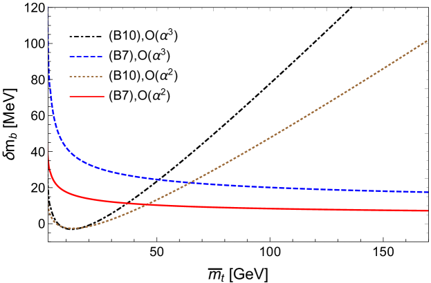
Refer to caption
Refer to caption
Figure 13: Upper panel: Plot of the correction to the PV mass of a top mass with varying m¯tsubscript¯𝑚𝑡{\overline{m}}_{t} mass due to a heavy quark with MS¯¯MS\overline{\rm MS} mass equal to 4.185 GeV (bottom) with and without decoupling (assuming a single heavy quark). Lower panel: As in the upper panel with a heavy quark with MS¯¯MS\overline{\rm MS} equal to 1.223 GeV (charm). We use Eqs. (78) and (81).

Let us now discuss in more detail the dependence on the bottom and charm quark, in particular the effects associated to the fact that they have masses much bigger than ΛQCDsubscriptΛQCD\Lambda_{\rm QCD} (for the analysis we take m¯b=4.186subscript¯𝑚𝑏4.186{\overline{m}}_{b}=4.186 GeV and m¯c=1.223subscript¯𝑚𝑐1.223{\overline{m}}_{c}=1.223 GeV Peset:2018ria but the sensitivity to the specific values we use is very tiny). As already discussed in Ball:1995ni , the natural scale of a n𝑛n-loop integral is not m¯tsubscript¯𝑚𝑡{\overline{m}}_{t} but m¯tensubscript¯𝑚𝑡superscript𝑒𝑛{\overline{m}}_{t}e^{-n}. For the case of the bottom versus charm quark it was observed in Ayala:2014yxa 666In that reference MeV should read GeV instead from Eq. (8) to Eq. (12). that the charm quark effectively decouples at order α2/α3superscript𝛼2superscript𝛼3\alpha^{2}/\alpha^{3} for the case of the charm quark effects in the bottom pole mass-MS¯¯MS\overline{\rm MS} mass relation. If we lower the mass of the top we can also observe at which scales it is more convenient to decouple the bottom and charm quark in the top pole mass-MS¯¯MS\overline{\rm MS} mass relation. This can be illustrated in Fig. 13, where we plot the corrections associated to the bottom and charm with and without decoupling in terms of the fictitious top mass (assuming a single heavy quark). Obviously for very large top masses it is not convenient to do the decoupling. Nevertheless, as we decrease the mass of the top it becomes much more effective to decouple, first the bottom, and afterwards the charm quark. Once this is done the corrections due to the bottom and charm masses to Eq. (59) are very small. Comparatively to other errors, the uncertainty associated to the 𝒪(α4)𝒪superscript𝛼4{\cal O}(\alpha^{4}) corrections is negligible. Also the correction associated to the bottom and charm quark masses to Eq. (58) is, comparatively to the total running, very small. From this analysis we will take as central values μb=20subscript𝜇𝑏20\mu_{b}=20 GeV and μc=5subscript𝜇𝑐5\mu_{c}=5 GeV. For these values we obtain

μbm¯t𝑑m¯ddm¯(δmb(5)(m¯)+δmc(5)(m¯)+δm(bc)(5)(m¯))subscriptsuperscriptsubscript¯𝑚𝑡subscript𝜇𝑏differential-d¯𝑚𝑑𝑑¯𝑚𝛿superscriptsubscript𝑚𝑏5¯𝑚𝛿superscriptsubscript𝑚𝑐5¯𝑚𝛿superscriptsubscript𝑚𝑏𝑐5¯𝑚\displaystyle\int^{{\overline{m}}_{t}}_{\mu_{b}}d{\overline{m}}\frac{d}{d{\overline{m}}}(\delta m_{b}^{(5)}({\overline{m}})+\delta m_{c}^{(5)}({\overline{m}})+\delta m_{(bc)}^{(5)}({\overline{m}})) (60)
+\displaystyle+ μcμb𝑑m¯ddm¯(δmb(4)(m¯)+δmc(4)(m¯)+δm(bc)(4)(m¯))subscriptsuperscriptsubscript𝜇𝑏subscript𝜇𝑐differential-d¯𝑚𝑑𝑑¯𝑚𝛿superscriptsubscript𝑚𝑏4¯𝑚𝛿superscriptsubscript𝑚𝑐4¯𝑚𝛿superscriptsubscript𝑚𝑏𝑐4¯𝑚\displaystyle\int^{\mu_{b}}_{\mu_{c}}d{\overline{m}}\frac{d}{d{\overline{m}}}(\delta m_{b}^{(4)}({\overline{m}})+\delta m_{c}^{(4)}({\overline{m}})+\delta m_{(bc)}^{(4)}({\overline{m}}))
+\displaystyle+ δmb(3)(μc)+δmc(3)(μc)+δm(bc)(3)(μc)=2.5|𝒪(α2)+0.8|𝒪(α3)=1.7MeV.𝛿subscriptsuperscript𝑚3𝑏subscript𝜇𝑐𝛿subscriptsuperscript𝑚3𝑐subscript𝜇𝑐𝛿subscriptsuperscript𝑚3𝑏𝑐subscript𝜇𝑐evaluated-at2.5𝒪superscript𝛼2evaluated-at0.8𝒪superscript𝛼31.7MeV\displaystyle\delta m^{(3)}_{b}(\mu_{c})+\delta m^{(3)}_{c}(\mu_{c})+\delta m^{(3)}_{(bc)}(\mu_{c})=-2.5\Bigg{|}_{{\cal O}(\alpha^{2})}+0.8\Bigg{|}_{{\cal O}(\alpha^{3})}=-1.7\;{\rm MeV}\,.

The specific value depends on μbsubscript𝜇𝑏\mu_{b} and μcsubscript𝜇𝑐\mu_{c} but the good convergence and smallness of this correction holds true for other values of μbsubscript𝜇𝑏\mu_{b} and μcsubscript𝜇𝑐\mu_{c}. The implementation of the decoupling of the bottom and charm in Hoang:2017btd produces a much larger correction. An even larger effect is observed in the implementation performed in Beneke:2016cbu , where the perturbative expansion is always performed at the scale of the top mass (using renormalon based estimates for the higher order coefficients), decoupling the bottom, and later the charm, depending on the order of perturbation theory. Therefore, we take our numbers as optima, and the error negligible compared with other uncertainties.

We next explore the convergence pattern of the perturbative expansion. We first consider the perturbative expansion associated to {\cal F}. We find

μbm¯t𝑑m¯(m¯,5)+μcμb𝑑m¯(m¯,4)=8445+837+5343=9291(22)MeV.subscriptsuperscriptsubscript¯𝑚𝑡subscript𝜇𝑏differential-d¯𝑚¯𝑚5subscriptsuperscriptsubscript𝜇𝑏subscript𝜇𝑐differential-d¯𝑚¯𝑚484458375343929122MeV\int^{{\overline{m}}_{t}}_{\mu_{b}}d{\overline{m}}{\cal F}({\overline{m}},5)+\int^{\mu_{b}}_{\mu_{c}}d{\overline{m}}{\cal F}({\overline{m}},4)=8445+837+53-43=9291(22)\;{\rm MeV}\,. (61)

We observe a convergent pattern. For the last two terms the convergence deteriorates. On the other hand the perturbative expansion becomes sign alternating. This may indicate sensitivity to the u=1𝑢1u=-1 renormalon. We discuss this further in the next section. For sign-alternating asymptotic perturbative expansion the left-over is 1/2×\sim-1/2\times(the last computed term) (see Dingle ).777We emphasize that these arguments do not apply to IR renormalons (and in particular to the u=1/2𝑢12u=1/2 renormalon). Therefore, we take it as the error of the truncation of the perturbative expansion, which is the error we quote in Eq. (61). We also explore the dependence of Eq. (58) on μbsubscript𝜇𝑏\mu_{b} and μcsubscript𝜇𝑐\mu_{c}. The dependence is very small, as we can see in Fig. 14. For μcsubscript𝜇𝑐\mu_{c} the variation is negligible, and for μbsubscript𝜇𝑏\mu_{b} one gets variations of 5similar-toabsent5\sim 5 MeV for a central value of μbsubscript𝜇𝑏\mu_{b} or around 20 GeV. Therefore, we will neglect it for the total error budget.

Refer to caption
Refer to caption
Figure 14: Plots of Eq. (58) in terms of μbsubscript𝜇𝑏\mu_{b} (upper panel) and μcsubscript𝜇𝑐\mu_{c} (lower panel) truncating the perturbative expansion of (m¯,nf)¯𝑚subscript𝑛𝑓{\cal F}({\overline{m}},n_{f}) at different orders in α𝛼\alpha in Eq. (61). In the upper figure we set μc=5subscript𝜇𝑐5\mu_{c}=5 GeV. In the lower figure we set μb=20subscript𝜇𝑏20\mu_{b}=20 GeV.

The other source of error is associated to the approximate determination of Eq. (59) (except for the δmq𝛿subscript𝑚𝑞\delta m_{q} terms, which have already been taken into account in Eq. (60)). The error analysis is equal to the one in Eq. (54) adapted by changing m¯b=4.186GeVμc=5subscript¯𝑚𝑏4.186GeVsubscript𝜇𝑐5{\overline{m}}_{b}=4.186\;{\rm GeV}\rightarrow\mu_{c}=5 GeV (the error associated to α𝛼\alpha is only computed for the full Eq. (58))

(mP(μc)+μcΩm)|μc=5GeV=5744(μ)15+7(Zm)9+9MeV.evaluated-atsubscript𝑚𝑃subscript𝜇𝑐subscript𝜇𝑐subscriptΩ𝑚subscript𝜇𝑐5GeV5744subscriptsuperscript𝜇715subscriptsuperscriptsubscript𝑍𝑚99MeV\left(m_{P}(\mu_{c})+\mu_{c}\Omega_{m}\right)\Bigg{|}_{\mu_{c}=5\;{\rm GeV}}=5744(\mu)^{+7}_{-15}(Z_{m})^{+9}_{-9}\;{\rm MeV}\,. (62)

Finally, we also include the error associated to α𝛼\alpha. Combining all errors we obtain

mt,PV(163MeV)=173033(h.o.)22+22(μ)15+7(Zm)9+9(α)123+119MeV.m_{t,\rm PV}(163{\rm MeV})=173033({\rm h.o.})^{+22}_{-22}(\mu)^{+7}_{-15}(Z_{m})^{+9}_{-9}(\alpha)^{+119}_{-123}\;{\rm MeV}\,. (63)

By far the largest uncertainty is associated to α𝛼\alpha. For the purely theoretical error budget, the error is associated to higher order corrections in perturbation theory. They show up in different ways. One is the approximate knowledge of Zmsubscript𝑍𝑚Z_{m}, which shows up in ΩmsubscriptΩ𝑚\Omega_{m}. The other is the error in μ𝜇\mu, which is a measure of the 𝒪(e2πβ0αX(μ)(1+ln(2)))𝒪superscript𝑒2𝜋subscript𝛽0subscript𝛼𝑋𝜇12{\cal O}(e^{-\frac{2\pi}{\beta_{0}\alpha_{X}(\mu)}(1+\ln(2))}) corrections to Eq. (59). h.o. stands for the error associated to higher order terms in perturbation theory of Eq. (61). All these errors would profit from higher order perturbative computations. We have also explored other sources of uncertainty, and find them to be comparatively very small: the error (and the effect) associated to the finite mass of the bottom and charm quark is found to be very small, and similarly for variations in the values of μbsubscript𝜇𝑏\mu_{b} and μcsubscript𝜇𝑐\mu_{c}.

It is also useful to make the error estimate of the ratio of the PV and MS¯¯MS\overline{\rm MS} top mass. We obtain (m¯t=163subscript¯𝑚𝑡163{\overline{m}}_{t}=163 GeV)

[mt,PVm¯t1]×105=6155(h.o.)13+13(μ)9+4(Zm)6+6(α)75+73.[\frac{m_{t,\rm PV}}{{\overline{m}}_{t}}-1]\times 10^{5}=6155({\rm h.o.})^{+13}_{-13}(\mu)^{+4}_{-9}(Z_{m})^{+6}_{-6}(\alpha)^{+73}_{-75}\,. (64)

Note that there is no ambiguity error associated to this number. Except for α𝛼\alpha all errors are associated to the lack of knowledge of higher order terms of the perturbative expansion. In comparison with Beneke:2016cbu we find that our result is less sensitive to Zmsubscript𝑍𝑚Z_{m} and to its associated error.

V.3 |u|=1𝑢1|u|=1 renormalons

The perturbative expansion of (m¯,nf)¯𝑚subscript𝑛𝑓{\cal F}({\overline{m}},n_{f}) is free of the u=1/2𝑢12u=1/2 renormalon. Therefore, it is the ideal object on which to study the subleading renormalons of the pole mass. In principle, these are located at u=1𝑢1u=1 and u=1𝑢1u=-1. The existence of an infrared renormalon at u=1𝑢1u=1 has been a matter of debate Neubert:1996zy . The existence of an ultraviolet renormalon at u=1𝑢1u=-1 can be established in the large β0subscript𝛽0\beta_{0} approximation Ball:1995ni ; Neubert:1994vb but not beyond. With respect to this discussion some interesting observations can be drawn out of our analysis. The coefficients fnsubscript𝑓𝑛f_{n} show an interesting dependence in nfsubscript𝑛𝑓n_{f} (with changes of sign of different powers of nfsubscript𝑛𝑓n_{f}). In Table 5 we give the numbers of fnsubscript𝑓𝑛f_{n} for different values of nfsubscript𝑛𝑓n_{f} and also in the large β0subscript𝛽0\beta_{0} approximation. We observe that for nf=3subscript𝑛𝑓3n_{f}=3 the 𝒪(α4)𝒪superscript𝛼4{\cal O}(\alpha^{4}) flips sign. For nf=6subscript𝑛𝑓6n_{f}=6, the 𝒪(α3)𝒪superscript𝛼3{\cal O}(\alpha^{3}) and 𝒪(α4)𝒪superscript𝛼4{\cal O}(\alpha^{4}) flip sign. The situation is somewhat puzzling. Let us first note that the sign of the coefficients would be interchanged compared with the large β0subscript𝛽0\beta_{0} predictions (for nf=3subscript𝑛𝑓3n_{f}=3). This could still be understood from a u=1𝑢1u=-1 renormalon if Z2Xsuperscriptsubscript𝑍2𝑋Z_{-2}^{X} flips sign from the large β0subscript𝛽0\beta_{0} prediction to real QCD. This would indicate a large dependence of Z2Xsuperscriptsubscript𝑍2𝑋Z_{-2}^{X} on nfsubscript𝑛𝑓n_{f} compared with what has been seen for ZmXsuperscriptsubscript𝑍𝑚𝑋Z_{m}^{X}, where the large β0subscript𝛽0\beta_{0} approximation gave the right sign and order of magnitude. For nfsubscript𝑛𝑓n_{f}\rightarrow\infty, the results agree with QED expectations (β0subscript𝛽0\beta_{0} becomes negative and the perturbative series is non sign-alternating). For nf=6subscript𝑛𝑓6n_{f}=6 we observe that the last two terms are negative. One may then wonder if what we are seeing for nf=6subscript𝑛𝑓6n_{f}=6 (and maybe also for nf=3subscript𝑛𝑓3n_{f}=3) is that the u=1𝑢1u=-1 renormalon becomes effectively infrared. Obviously, we need higher order coefficients fnsubscript𝑓𝑛f_{n} to clarify this issue.888The coefficients of the perturbative expansion of the pole mass itself are also a polynomial in powers of nfsubscript𝑛𝑓n_{f}. The sign dependence of the different powers of nfsubscript𝑛𝑓n_{f} has been studied in Kataev:2018gle ; Kataev:2018mob .

(m¯,nf)¯𝑚subscript𝑛𝑓{\cal F}({\overline{m}},n_{f}) f1subscript𝑓1f_{1} f2subscript𝑓2f_{2} f3subscript𝑓3f_{3} f4subscript𝑓4f_{4} f5subscript𝑓5f_{5}
nf=0subscript𝑛𝑓0n_{f}=0 4/3434/3 6.116.116.11 25.5225.5225.52 18.4618.4618.46
nf=3subscript𝑛𝑓3n_{f}=3 4/3434/3 4.324.324.32 12.7612.7612.76 63.3763.37-63.37
nf=6subscript𝑛𝑓6n_{f}=6 4/3434/3 2.532.532.53 0.740.74-0.74 105.70105.70-105.70
(Large β0subscript𝛽0\beta_{0}/exact) nf=1020subscript𝑛𝑓superscript1020n_{f}=10^{20} 4/3434/3 5.97×10195.97superscript1019-5.97\times 10^{19} 4.15×10384.15superscript1038-4.15\times 10^{38} 2.54×10582.54superscript1058-2.54\times 10^{58} 5.09×10775.09superscript1077-5.09\times 10^{77}
(Large β0subscript𝛽0\beta_{0}) nf=0subscript𝑛𝑓0n_{f}=0 4/3434/3 9.859.859.85 11.3111.31-11.31 114.33114.33114.33 -377.22
(Large β0subscript𝛽0\beta_{0}) nf=3subscript𝑛𝑓3n_{f}=3 4/3434/3 8.068.068.06 7.577.57-7.57 62.6262.6262.62 -169.04
(Large β0subscript𝛽0\beta_{0}) nf=6subscript𝑛𝑓6n_{f}=6 4/3434/3 6.276.276.27 4.584.58-4.58 29.4629.4629.46 -61.86
Table 5: The coefficients fnsubscript𝑓𝑛f_{n} of (m¯,nf)¯𝑚subscript𝑛𝑓{\cal F}({\overline{m}},n_{f}). Note that f4(nf=0)subscript𝑓4subscript𝑛𝑓0f_{4}(n_{f}=0) has a 9%percent99\% error from the determination in Marquard:2015qpa . The nf=1020subscript𝑛𝑓superscript1020n_{f}=10^{20} case is used as a test for comparison with the large β0subscript𝛽0\beta_{0}. The last three (four) rows are the coefficients fnsubscript𝑓𝑛f_{n} in the large β0subscript𝛽0\beta_{0} approximation.

It is usual lore that infrared renormalons dominate over ultraviolet ones (this is somewhat based on large β0subscript𝛽0\beta_{0} analyses where ultraviolet renormalons are typically suppressed by the factor edcX2similar-toabsentsuperscript𝑒𝑑subscript𝑐𝑋2\sim e^{d\frac{c_{X}}{2}} whereas infrared renormalons are enhanced by the factor edcX2similar-toabsentsuperscript𝑒𝑑subscript𝑐𝑋2\sim e^{-d\frac{c_{X}}{2}}). If we take this seriously, and also the numbers we obtain for fnsubscript𝑓𝑛f_{n} as an indication of the existence of the u=1𝑢1u=-1 renormalon, this may indicate that the u=1𝑢1u=1 renormalon is indeed zero. In this respect, it is worth mentioning the analysis of Bazavov:2018omf where the NP correction associated to the u=1𝑢1u=1 renormalon was found to be zero within errors. This is consistent with this discussion.

On the theoretical side it is also interesting to see where the u=1𝑢1u=1 renormalon would show up in a perturbative computation of the heavy quarkonium mass. For the purposes of this discussion, the heavy quarkonium mass would read

Mnl=2mQ+𝐩2mQnl+V0nl+V1mQnl+𝒪(1mQ2),subscript𝑀𝑛𝑙2subscript𝑚𝑄subscriptdelimited-⟨⟩superscript𝐩2subscript𝑚𝑄𝑛𝑙subscriptdelimited-⟨⟩subscript𝑉0𝑛𝑙subscriptdelimited-⟨⟩subscript𝑉1subscript𝑚𝑄𝑛𝑙𝒪1superscriptsubscript𝑚𝑄2M_{nl}=2m_{Q}+\langle\frac{{\bf p}^{2}}{m_{Q}}\rangle_{nl}+\langle V_{0}\rangle_{nl}+\langle\frac{V_{1}}{m_{Q}}\rangle_{nl}+{\cal O}\left(\frac{1}{m_{Q}^{2}}\right)\,, (65)

where V0subscript𝑉0V_{0} is the static potential, and V1subscript𝑉1V_{1} is the 1/mQ1subscript𝑚𝑄1/m_{Q} potential. OPE analyses in the static limit show that V0subscript𝑉0V_{0} does not have renormalon at u=1𝑢1u=1. The virial theorem: 𝐩2mQnl=rV0nlsubscriptdelimited-⟨⟩superscript𝐩2subscript𝑚𝑄𝑛𝑙subscriptdelimited-⟨⟩𝑟subscriptsuperscript𝑉0𝑛𝑙\langle\frac{{\bf p}^{2}}{m_{Q}}\rangle_{nl}=\langle rV^{\prime}_{0}\rangle_{nl}, also guaranties that the kinetic term does not have such u=1𝑢1u=1 renormalon. Therefore, any possible u=1𝑢1u=1 infrared renormalon of the pole mass should cancel with the analogous infrared renormalon of the V1/mQsubscript𝑉1subscript𝑚𝑄V_{1}/m_{Q} potential. The fact that the latter can be written in a closed way in terms of Wilson loops Brambilla:2000gk may open a venue on which to study this issue in further detail. This is postponed to future work.

VI Conclusions

In this paper we have constructed hyperasymptotic expansions for the heavy quark pole mass (and for associated quantities) regulated using the PV prescription along the lines of HyperI . We generalize the discussion of that reference by including possible ultraviolet renormalons. Such organization of the computation allows us to have a parametric control of the error committed when truncating the hyperasymptotic expansion.

In Sec. III the hyperasymptotic expansion of the pole mass of a heavy quark in the large β0subscript𝛽0\beta_{0} is computed. We use it as a toy-model observable to test our methods. It works as expected. We can see the u=1/2𝑢12u=1/2 infrared renormalon and the u=1𝑢1u=-1 ultraviolet renormalon. The next infrared renormalon is located at u=3/2𝑢32u=3/2. Compared with the static potential case studied in HyperI in the large β0subscript𝛽0\beta_{0} approximation, infrared renormalons are located at the same points in the Borel plane. On the other hand, the pole mass has ultraviolet renormalons, whereas the static potential does not. In practice the main difference comes from the relevance of the u=1𝑢1u=-1 renormalon. In general, because of the u=1𝑢1u=-1 renormalon, it is necessary to stop the second perturbative expansion (see Eq. (19)) at N2×2πβ0αsimilar-to𝑁22𝜋subscript𝛽0𝛼N\sim 2\times\frac{2\pi}{\beta_{0}\alpha}, otherwise the perturbative series would start to diverge, as we can observe in Fig. 7 in the MS¯¯MS\overline{\rm MS} scheme. Nevertheless, the importance of this renormalon heavily depends on the factorization scale μ𝜇\mu one uses. If one takes μ𝜇\mu high enough, one could indeed do perturbation theory until N3×2πβ0αsimilar-to𝑁32𝜋subscript𝛽0𝛼N\sim 3\times\frac{2\pi}{\beta_{0}\alpha}, where the u=3/2𝑢32u=3/2 renormalon shows up. We can see the irrelevance of the u=1𝑢1u=-1 renormalon in the lattice scheme, which is equivalent to the MS¯¯MS\overline{\rm MS} scheme with a much larger μ𝜇\mu, in Fig. 7. One should keep in mind, though, that one needs perturbation theory to a much higher order in the lattice scheme to reach the same precision than in the MS¯¯MS\overline{\rm MS} scheme. We expect this qualitative behavior of ultraviolet renormalons to also hold true beyond the large β0subscript𝛽0\beta_{0} approximation.

We next move to real QCD. We have performed determinations of Λ¯PVsubscript¯ΛPV\bar{\Lambda}_{\rm PV} using quenched lattice QCD. For these observables perturbative expansions to high orders are available Bauer:2011ws ; Bali:2013pla ; Bali:2013qla . This allows us to test the method and go beyond the superasymptotic and the leading term in the hyperasymptotic approximation. We observe 𝒪(aΛQCD2)𝒪𝑎superscriptsubscriptΛQCD2{\cal O}(a\Lambda_{\rm QCD}^{2}) corrections for the B𝐵B meson mass in the static approximation, but not for an analogous observable from the static potential. Nevertheless, we do not have enough precision to quantitatively study these effects. The limiting factor is the error of the normalization of the leading renormalon, and, related, the lack of knowledge of the higher order beta function coefficients. The latter affects the 𝒪(1/n)𝒪1𝑛{\cal O}(1/n) corrections to the asymptotic formula of the perturbative series coefficients. These effects are sizable in the lattice scheme. On the other hand they are quite small in the MS¯¯MS\overline{\rm MS} scheme. On top of that the higher order coefficients of the perturbative expansion of δmlatt𝛿subscript𝑚latt\delta m_{\rm latt} are not known with enough precision to disentangle the subleading renormalon (their error is strongly correlated with the error of Zmsubscript𝑍𝑚Z_{m}). All these considerations forbid quantitative analyses beyond the leading term in the hyperasymptotic approximation. Further investigations are needed to improve on these issues, particularly on the error of Zmsubscript𝑍𝑚Z_{m}, which also affects the discussion below.

We also determine Λ¯PVsubscript¯ΛPV\bar{\Lambda}_{\rm PV} from the physical B𝐵B meson mass assuming that the MS¯¯MS\overline{\rm MS} heavy quark mass is known. The result can be found in Eq. (54). In this analysis, we determine the error associated to the incomplete knowledge of the perturbative expansion in determinations of the heavy quark mass. We translate this result to the case of the top mass, which we study in detail in Sec. V. In this section the issue of the uncertainty of the (top) pole mass is critically reexamined. In particular, the bottom and charm quark finite mass effects are carefully incorporated. In our implementation we find these to be very small. We find the present uncertainty in the relation between m¯tsubscript¯𝑚𝑡{\overline{m}}_{t} and mPVsubscript𝑚PVm_{\rm PV} to be (for m¯t=163subscript¯𝑚𝑡163{\overline{m}}_{t}=163 GeV)

mt,PV(163MeV)=173033(th)28+25(α)123+119MeV,subscript𝑚𝑡PV163MeV173033subscriptsuperscriptth2528subscriptsuperscript𝛼119123MeVm_{t,\rm PV}(163{\rm MeV})=173033({\rm th})^{+25}_{-28}(\alpha)^{+119}_{-123}\;{\rm MeV}\,, (66)
[mt,PVm¯t1]×105=6155(th)17+15(α)75+73,delimited-[]subscript𝑚𝑡PVsubscript¯𝑚𝑡1superscript1056155subscriptsuperscriptth1517subscriptsuperscript𝛼7375[\frac{m_{t,\rm PV}}{{\overline{m}}_{t}}-1]\times 10^{5}=6155\,({\rm th})^{+15}_{-17}\,(\alpha)^{+73}_{-75}\,, (67)

where we have combined the theoretical errors quoted in Eqs. (63) and (64) in quadrature. There is no ambiguity associated to the renormalon in this number. The precision is systematically improvable the more terms of the perturbative expansion get to be known in the future. Interestingly enough, it seems we have found some evidence for the existence of the next renormalon at u=1𝑢1u=-1 but not of a possible renormalon at u=1𝑢1u=1. We believe this makes very timely a quantitative determination of the renormalization group structure of the u=1𝑢1u=-1 renormalon, which to our knowledge is lacking. We leave this for future work.

Acknowledgments
We thank M. Steinhauser for comments on the manuscript. C.A. thanks the IFAE group at Universitat Autònoma de Barcelona for warm hospitality during part of this work. This work was supported in part by the Spanish FPA2017-86989-P and SEV-2016-0588 grants from the ministerio de Ciencia, Innovación y Universidades, and the 2017SGR1069 grant from the Generalitat de Catalunya; and by the Chilean FONDECYT Postdoctoral Grant No. 3170116, and by FONDECYT Regular Grant No. 1180344.

Appendix A Evaluation of ΩdsubscriptΩ𝑑\Omega_{d}

We here briefly sketch how we compute the integrals that appear in ΩdsubscriptΩ𝑑\Omega_{d}. For d<0𝑑0d<0 we use the recursion formulas developed in Dingle (see for instance Eq. (46) of Chapter XXI). For d>0𝑑0d>0, we can use also such formulas (see for instance Eq. (47) of Chapter XXI). In this case, we can also alternatively perform the integration in the following way. For simplicity, we take the case b=0𝑏0b=0 and d=1𝑑1d=1, as the method is similar for the more general case.

I=0,PV𝑑ue4πβ0αu(2u)N+112u=12e2πβ0α12,PVdyye4πβ0αye(2πβ0α(1cα)+1)ln(1+2y),𝐼superscriptsubscript0PVdifferential-d𝑢superscript𝑒4𝜋subscript𝛽0𝛼𝑢superscript2𝑢𝑁112𝑢12superscript𝑒2𝜋subscript𝛽0𝛼superscriptsubscript12PV𝑑𝑦𝑦superscript𝑒4𝜋subscript𝛽0𝛼𝑦superscript𝑒2𝜋subscript𝛽0𝛼1𝑐𝛼112𝑦I=\int_{0,\rm PV}^{\infty}due^{-\frac{4\pi}{\beta_{0}\alpha}u}\frac{(2u)^{N+1}}{1-2u}=-\frac{1}{2}e^{-\frac{2\pi}{\beta_{0}\alpha}}\int_{-\frac{1}{2},\rm PV}^{\infty}\frac{dy}{y}e^{-\frac{4\pi}{\beta_{0}\alpha}y}e^{\left(\frac{2\pi}{\beta_{0}\alpha}(1-c\alpha)+1\right)\ln(1+2y)}\,, (68)

where in the second equality we set N=NP𝑁subscript𝑁𝑃N=N_{P} according to Eq. (3). We also do the change of variables (where K=cβ02π𝐾𝑐subscript𝛽02𝜋K=c-\frac{\beta_{0}}{2\pi})

y=x211Kαβ0απ.𝑦𝑥211𝐾𝛼subscript𝛽0𝛼𝜋y=\frac{x}{2}\frac{1}{\sqrt{1-K\alpha}}\sqrt{\frac{\beta_{0}\alpha}{\pi}}\,. (69)

We can then expand the exponent in powers of α𝛼\alpha and x𝑥x:

I=12e2πβ0απβ0α(1Kα),PVdxxex2e4πβ0αKx2β0απ11Kα+23x3β0απ11Kα+.𝐼12superscript𝑒2𝜋subscript𝛽0𝛼superscriptsubscript𝜋subscript𝛽0𝛼1𝐾𝛼PV𝑑𝑥𝑥superscript𝑒superscript𝑥2superscript𝑒4𝜋subscript𝛽0𝛼𝐾𝑥2subscript𝛽0𝛼𝜋11𝐾𝛼23superscript𝑥3subscript𝛽0𝛼𝜋11𝐾𝛼I=-\frac{1}{2}e^{-\frac{2\pi}{\beta_{0}\alpha}}\int_{-\sqrt{\frac{\pi}{\beta_{0}\alpha}(1-K\alpha)},\rm PV}^{\infty}\frac{dx}{x}e^{-x^{2}}e^{-\frac{4\pi}{\beta_{0}\alpha}K\frac{x}{2}\sqrt{\frac{\beta_{0}\alpha}{\pi}}\frac{1}{\sqrt{1-K\alpha}}+\frac{2}{3}x^{3}\sqrt{\frac{\beta_{0}\alpha}{\pi}}\frac{1}{\sqrt{1-K\alpha}}+\cdots}\,. (70)

The inferior limit of the integral is then extended to -\infty. We then have

I𝐼\displaystyle I similar-to-or-equals\displaystyle\simeq 12e2πβ0α,PVdxxex2e4πβ0αKx2β0απ11Kα+23x3β0απ11Kα+12superscript𝑒2𝜋subscript𝛽0𝛼superscriptsubscriptPV𝑑𝑥𝑥superscript𝑒superscript𝑥2superscript𝑒4𝜋subscript𝛽0𝛼𝐾𝑥2subscript𝛽0𝛼𝜋11𝐾𝛼23superscript𝑥3subscript𝛽0𝛼𝜋11𝐾𝛼\displaystyle-\frac{1}{2}e^{-\frac{2\pi}{\beta_{0}\alpha}}\int_{-\infty,\rm PV}^{\infty}\frac{dx}{x}e^{-x^{2}}e^{-\frac{4\pi}{\beta_{0}\alpha}K\frac{x}{2}\sqrt{\frac{\beta_{0}\alpha}{\pi}}\frac{1}{\sqrt{1-K\alpha}}+\frac{2}{3}x^{3}\sqrt{\frac{\beta_{0}\alpha}{\pi}}\frac{1}{\sqrt{1-K\alpha}}+\cdots} (71)
similar-to-or-equals\displaystyle\simeq e2πβ0α16β0α(1+6πβ0K)+.superscript𝑒2𝜋subscript𝛽0𝛼16subscript𝛽0𝛼16𝜋subscript𝛽0𝐾\displaystyle e^{-\frac{2\pi}{\beta_{0}\alpha}}\frac{1}{6}\sqrt{\beta_{0}\alpha}\left(-1+\frac{6\pi}{\beta_{0}}K\right)+\cdots\,.

Irrespectively of considering d>0𝑑0d>0 or d>0𝑑0d>0, it is not clear to us what is the asymptotic structure of this expansion. This is something that we are investigating. In any case, at present, we have not seen evidence of asymptotic behavior of this expansion for all cases we have considered. This does not preclude however that if we go to higher orders we will find an asymptotic behavior for this perturbative expansion.

Appendix B bottom and charm finite mass contributions to mt,PVsubscript𝑚𝑡PVm_{t,\rm PV}

We define

δmq(1)𝛿superscriptsubscript𝑚𝑞1\displaystyle\delta m_{q}^{(1)} \displaystyle\equiv m¯3((1m¯qm¯)(1m¯q3m¯3)(Li2(m¯qm¯)12ln2(m¯qm¯)+ln(1m¯qm¯)\displaystyle\frac{{{\overline{m}}}}{3}\left(\left(1-\frac{{{\overline{m}}}_{q}}{{{\overline{m}}}}\right)\left(1-\frac{{{\overline{m}}}_{q}^{3}}{{{\overline{m}}}^{3}}\right)\left(\text{Li}_{2}\left(\frac{{{\overline{m}}}_{q}}{{{\overline{m}}}}\right)-\frac{1}{2}{\rm ln}^{2}\left(\frac{{{\overline{m}}}_{q}}{{{\overline{m}}}}\right)+{\rm ln}\left(1-\frac{{{\overline{m}}}_{q}}{{{\overline{m}}}}\right)\right.\right. (72)
×ln(m¯qm¯)π23)+(1+m¯qm¯)(1+m¯q3m¯3)(Li2(m¯qm¯)12ln2(m¯qm¯)\displaystyle\left.\left.\times{\rm ln}\left(\frac{{{\overline{m}}}_{q}}{{{\overline{m}}}}\right)-\frac{\pi^{2}}{3}\right)+\left(1+\frac{{{\overline{m}}}_{q}}{{{\overline{m}}}}\right)\left(1+\frac{{{\overline{m}}}_{q}^{3}}{{{\overline{m}}}^{3}}\right)\left(\text{Li}_{2}\left(-\frac{{{\overline{m}}}_{q}}{{{\overline{m}}}}\right)-\frac{1}{2}{\rm ln}^{2}\left(\frac{{{\overline{m}}}_{q}}{{{\overline{m}}}}\right)\right.\right.
+ln(1+m¯qm¯)ln(m¯qm¯)+π26)m¯q2m¯2(ln(m¯qm¯)+32)+ln2(m¯qm¯)\displaystyle\left.\left.+{\rm ln}\left(1+\frac{{{\overline{m}}}_{q}}{{{\overline{m}}}}\right){\rm ln}\left(\frac{{{\overline{m}}}_{q}}{{{\overline{m}}}}\right)+\frac{\pi^{2}}{6}\right)-\frac{{{\overline{m}}}_{q}^{2}}{{{\overline{m}}}^{2}}\left({\rm ln}\left(\frac{{{\overline{m}}}_{q}}{{{\overline{m}}}}\right)+\frac{3}{2}\right)+{\rm ln}^{2}\left(\frac{{{\overline{m}}}_{q}}{{{\overline{m}}}}\right)\right.
+π26)\displaystyle\left.+\frac{\pi^{2}}{6}\right)

(note that this coefficient is nfsubscript𝑛𝑓n_{f}-independent),

δmq(2,nf)𝛿superscriptsubscript𝑚𝑞2subscript𝑛𝑓\displaystyle\delta m_{q}^{(2,n_{f})} =\displaystyle= m¯64[h(m¯qm¯)+w(1,m¯qm¯)+nfp(m¯qm¯)],¯𝑚64delimited-[]subscript¯𝑚𝑞¯𝑚𝑤1subscript¯𝑚𝑞¯𝑚subscript𝑛𝑓𝑝subscript¯𝑚𝑞¯𝑚\displaystyle\frac{{{\overline{m}}}}{64}\left[h\left(\frac{{{\overline{m}}}_{q}}{{{\overline{m}}}}\right)+w\left(1,\frac{{{\overline{m}}}_{q}}{{{\overline{m}}}}\right)+n_{f}\ p\left(\frac{{{\overline{m}}}_{q}}{{{\overline{m}}}}\right)\right]\,, (73)

where nf=5subscript𝑛𝑓5n_{f}=5 for q=b𝑞𝑏q=b and nf=4subscript𝑛𝑓4n_{f}=4 for q=c𝑞𝑐q=c, and we use the representation for the functions h(x)𝑥h(x), w(x,y)𝑤𝑥𝑦w(x,y) and p(x)𝑝𝑥p(x) given in Ref. Hoang:2017btd , and

δmbc(2)=m¯64w(m¯bm¯,m¯cm¯).𝛿superscriptsubscript𝑚𝑏𝑐2¯𝑚64𝑤subscript¯𝑚𝑏¯𝑚subscript¯𝑚𝑐¯𝑚\delta m_{bc}^{(2)}=\frac{{\overline{m}}}{64}\ w\left(\frac{{\overline{m}}_{b}}{{\overline{m}}},\frac{{\overline{m}}_{c}}{{\overline{m}}}\right)\,. (74)

We then have

δmb/c(5)𝛿superscriptsubscript𝑚𝑏𝑐5\displaystyle\delta m_{b/c}^{(5)} =\displaystyle= δmb/c(1)α(5)2(m¯)π2+δmb/c(2,5/4)α(5)3(m¯)π3𝛿superscriptsubscript𝑚𝑏𝑐1superscriptsubscript𝛼52¯𝑚superscript𝜋2𝛿subscriptsuperscript𝑚254𝑏𝑐superscriptsubscript𝛼53¯𝑚superscript𝜋3\displaystyle\delta m_{b/c}^{(1)}\frac{\alpha_{(5)}^{2}({\overline{m}})}{\pi^{2}}+\delta m^{(2,5/4)}_{b/c}\frac{\alpha_{(5)}^{3}({\overline{m}})}{\pi^{3}} (75)
δmbc(5)𝛿superscriptsubscript𝑚𝑏𝑐5\displaystyle\delta m_{bc}^{(5)} =\displaystyle= δmbc(2)α(5)3(m¯)π3𝛿subscriptsuperscript𝑚2𝑏𝑐superscriptsubscript𝛼53¯𝑚superscript𝜋3\displaystyle\delta m^{(2)}_{bc}\frac{\alpha_{(5)}^{3}({\overline{m}})}{\pi^{3}} (76)
δmb(4)𝛿superscriptsubscript𝑚𝑏4\displaystyle\delta m_{b}^{(4)} =\displaystyle= [δmb(1)+δmb,dec(1)]α(4)2(m¯)π2+[δmb(2,5)+δmb,dec(2)]α(4)3(m¯)π3delimited-[]𝛿superscriptsubscript𝑚𝑏1𝛿superscriptsubscript𝑚𝑏𝑑𝑒𝑐1superscriptsubscript𝛼42¯𝑚superscript𝜋2delimited-[]𝛿subscriptsuperscript𝑚25𝑏𝛿superscriptsubscript𝑚𝑏𝑑𝑒𝑐2superscriptsubscript𝛼43¯𝑚superscript𝜋3\displaystyle\left[\delta m_{b}^{(1)}+\delta m_{b,dec}^{(1)}\right]\frac{\alpha_{(4)}^{2}({\overline{m}})}{\pi^{2}}+\left[\delta m^{(2,5)}_{b}+\delta m_{b,dec}^{(2)}\right]\frac{\alpha_{(4)}^{3}({\overline{m}})}{\pi^{3}} (77)
δmc(4)𝛿superscriptsubscript𝑚𝑐4\displaystyle\delta m_{c}^{(4)} =\displaystyle= δmc(1)α(4)2(m¯)π2+δmc(2,4)α(4)3(m¯)π3𝛿superscriptsubscript𝑚𝑐1superscriptsubscript𝛼42¯𝑚superscript𝜋2𝛿subscriptsuperscript𝑚24𝑐superscriptsubscript𝛼43¯𝑚superscript𝜋3\displaystyle\delta m_{c}^{(1)}\frac{\alpha_{(4)}^{2}({\overline{m}})}{\pi^{2}}+\delta m^{(2,4)}_{c}\frac{\alpha_{(4)}^{3}({\overline{m}})}{\pi^{3}} (78)
δmbc(4)𝛿superscriptsubscript𝑚𝑏𝑐4\displaystyle\delta m_{bc}^{(4)} =\displaystyle= [δmbc(2)+δmbc,dec(2)]α(4)3(m¯)π3delimited-[]𝛿subscriptsuperscript𝑚2𝑏𝑐𝛿subscriptsuperscript𝑚2𝑏𝑐𝑑𝑒𝑐superscriptsubscript𝛼43¯𝑚superscript𝜋3\displaystyle\left[\delta m^{(2)}_{bc}+\delta m^{(2)}_{bc,dec}\right]\frac{\alpha_{(4)}^{3}({\overline{m}})}{\pi^{3}} (79)
δmb(3)𝛿superscriptsubscript𝑚𝑏3\displaystyle\delta m_{b}^{(3)} =\displaystyle= [δmb(1)+δmb,dec(1)]α(3)2(m¯)π2+[δmb(2,5)+δmb,dec(2)]α(3)3(m¯)π3delimited-[]𝛿superscriptsubscript𝑚𝑏1𝛿superscriptsubscript𝑚𝑏𝑑𝑒𝑐1superscriptsubscript𝛼32¯𝑚superscript𝜋2delimited-[]𝛿subscriptsuperscript𝑚25𝑏𝛿superscriptsubscript𝑚𝑏𝑑𝑒𝑐2superscriptsubscript𝛼33¯𝑚superscript𝜋3\displaystyle\left[\delta m_{b}^{(1)}+\delta m_{b,dec}^{(1)}\right]\frac{\alpha_{(3)}^{2}({\overline{m}})}{\pi^{2}}+\left[\delta m^{(2,5)}_{b}+\delta m_{b,dec}^{(2)}\right]\frac{\alpha_{(3)}^{3}({\overline{m}})}{\pi^{3}} (80)
δmc(3)𝛿superscriptsubscript𝑚𝑐3\displaystyle\delta m_{c}^{(3)} =\displaystyle= [δmc(1)+δmc,dec(1)]α(3)2(m¯)π2+[δmc(2,4)+δmc,dec(2)]α(3)3(m¯)π3delimited-[]𝛿superscriptsubscript𝑚𝑐1𝛿superscriptsubscript𝑚𝑐𝑑𝑒𝑐1superscriptsubscript𝛼32¯𝑚superscript𝜋2delimited-[]𝛿subscriptsuperscript𝑚24𝑐𝛿superscriptsubscript𝑚𝑐𝑑𝑒𝑐2superscriptsubscript𝛼33¯𝑚superscript𝜋3\displaystyle\left[\delta m_{c}^{(1)}+\delta m_{c,dec}^{(1)}\right]\frac{\alpha_{(3)}^{2}({\overline{m}})}{\pi^{2}}+\left[\delta m^{(2,4)}_{c}+\delta m_{c,dec}^{(2)}\right]\frac{\alpha_{(3)}^{3}({\overline{m}})}{\pi^{3}} (81)
δmbc(3)𝛿superscriptsubscript𝑚𝑏𝑐3\displaystyle\delta m_{bc}^{(3)} =\displaystyle= [δmbc(2)+δmbc,dec(2)+δmcb,dec(2)]α(3)3(m¯)π3,delimited-[]𝛿subscriptsuperscript𝑚2𝑏𝑐𝛿subscriptsuperscript𝑚2𝑏𝑐𝑑𝑒𝑐𝛿subscriptsuperscript𝑚2𝑐𝑏𝑑𝑒𝑐superscriptsubscript𝛼33¯𝑚superscript𝜋3\displaystyle\left[\delta m^{(2)}_{bc}+\delta m^{(2)}_{bc,dec}+\delta m^{(2)}_{cb,dec}\right]\frac{\alpha_{(3)}^{3}({\overline{m}})}{\pi^{3}}\,, (82)

where δm(q,dec)(i)𝛿superscriptsubscript𝑚𝑞dec𝑖\delta m_{(q,\rm dec)}^{(i)} are generated by the decoupling and read

δm(q,dec)(1)=29m¯(7132+ln(m¯q2m¯2)+π24),𝛿superscriptsubscript𝑚𝑞dec129¯𝑚7132lnsuperscriptsubscript¯𝑚𝑞2superscript¯𝑚2superscript𝜋24\displaystyle\delta m_{(q,\rm dec)}^{(1)}=-\frac{2}{9}{{\overline{m}}}\left(\frac{71}{32}+{\rm ln}\left(\frac{{\overline{m}}_{q}^{2}}{{\overline{m}}^{2}}\right)+\frac{\pi^{2}}{4}\right)\,, (83)
δm(q,dec)(2,nf)𝛿superscriptsubscript𝑚𝑞𝑑𝑒𝑐2subscript𝑛𝑓\displaystyle\delta m_{(q,dec)}^{(2,n_{f})} =\displaystyle= m¯{[235311664+727ζ(3)+13π2162(π254+71432)ln(m¯2m¯q2)]nf+8Li4(12)27\displaystyle{{\overline{m}}}\left\{\left[\frac{2353}{11664}+\frac{7}{27}\zeta(3)+\frac{13\pi^{2}}{162}-\left(\frac{\pi^{2}}{54}+\frac{71}{432}\right){\rm ln}\left(\frac{{{\overline{m}}}^{2}}{{{\overline{m}}}_{q}^{2}}\right)\right]n_{f}+\frac{8\text{Li}_{4}\left(\frac{1}{2}\right)}{27}\right. (84)
751216ζ(3)+61π41944113π272298692916+ln4(2)81+281π2ln2(2)1181π2ln(2)751216𝜁361superscript𝜋41944113superscript𝜋272298692916superscriptln4281281superscript𝜋2superscriptln221181superscript𝜋2ln2\displaystyle\left.-\frac{751}{216}\zeta(3)+\frac{61\pi^{4}}{1944}-\frac{113\pi^{2}}{72}-\frac{29869}{2916}+\frac{{\rm ln}^{4}(2)}{81}+\frac{2}{81}\pi^{2}{\rm ln}^{2}(2)-\frac{11}{81}\pi^{2}{\rm ln}(2)\right.
+(1225288118ζ(3)+π29+127π2ln(2))ln(m¯2m¯q2)+127ln2(m¯2m¯q2)}\displaystyle\left.+\left(\frac{1225}{288}-\frac{1}{18}\zeta(3)+\frac{\pi^{2}}{9}+\frac{1}{27}\pi^{2}{\rm ln}(2)\right){\rm ln}\left(\frac{{{\overline{m}}}^{2}}{{{\overline{m}}}_{q}^{2}}\right)+\frac{1}{27}{\rm ln}^{2}\left(\frac{{{\overline{m}}}^{2}}{{{\overline{m}}}_{q}^{2}}\right)\right\}
+13ln(m¯2m¯q2)δmq(1).13lnsuperscript¯𝑚2superscriptsubscript¯𝑚𝑞2𝛿superscriptsubscript𝑚𝑞1\displaystyle+\frac{1}{3}{\rm ln}\left(\frac{{{\overline{m}}}^{2}}{{{\overline{m}}}_{q}^{2}}\right)\delta m_{q}^{(1)}\,.

Note that δm(b,dec)(2)=δm(b,dec)(2,5)𝛿superscriptsubscript𝑚𝑏𝑑𝑒𝑐2𝛿superscriptsubscript𝑚𝑏𝑑𝑒𝑐25\delta m_{(b,dec)}^{(2)}=\delta m_{(b,dec)}^{(2,5)} and δm(c,dec)(2)=δm(b,dec)(2,4)𝛿superscriptsubscript𝑚𝑐𝑑𝑒𝑐2𝛿superscriptsubscript𝑚𝑏𝑑𝑒𝑐24\delta m_{(c,dec)}^{(2)}=\delta m_{(b,dec)}^{(2,4)}. This last expression indeed corresponds to Eq. (17) of Ayala:2014yxa changing m¯bsubscript¯𝑚𝑏{\overline{m}}_{b} by m¯¯𝑚{\overline{m}}.

Finally, we also have

δmbc,dec(2)=13ln(m¯2m¯b2)δmc(1),𝛿subscriptsuperscript𝑚2𝑏𝑐𝑑𝑒𝑐13superscript¯𝑚2superscriptsubscript¯𝑚𝑏2𝛿superscriptsubscript𝑚𝑐1\delta m^{(2)}_{bc,dec}=\frac{1}{3}\ln\left(\frac{{\overline{m}}^{2}}{{\overline{m}}_{b}^{2}}\right)\delta m_{c}^{(1)}\,, (85)
δmcb,dec(2)=13ln(m¯2m¯c2)[δmb(1)+δmb,dec(1)].𝛿subscriptsuperscript𝑚2𝑐𝑏𝑑𝑒𝑐13superscript¯𝑚2superscriptsubscript¯𝑚𝑐2delimited-[]𝛿superscriptsubscript𝑚𝑏1𝛿superscriptsubscript𝑚𝑏𝑑𝑒𝑐1\delta m^{(2)}_{cb,dec}=\frac{1}{3}\ln\left(\frac{{\overline{m}}^{2}}{{\overline{m}}_{c}^{2}}\right)[\delta m_{b}^{(1)}+\delta m_{b,dec}^{(1)}]\,. (86)

References

  • (1) C. Ayala, X. Lobregat and A. Pineda, Phys. Rev. D 99, no. 7, 074019 (2019) [arXiv:1902.07736 [hep-th]].
  • (2) M. V. Berry and C. J. Howls, Hyperasymptotics, Proc. Roy. Soc. London A, 430 (1990), pp. 653-668.
  • (3) J. P. Boyd, The Devil’s Invention: Asymptotic, Superasymptotic and Hyperasymptotic Series, Acta Applicandae Mathematica, Vol. 56, 1 (1999).
  • (4) C. Ayala, X. Lobregat and A. Pineda, arXiv:1910.04090 [hep-ph].
  • (5) R.B. Dingle, Asymptotic Expansions: Their Derivation and Interpretation (Academic Press, London, 1973).
  • (6) R. Tarrach, Nucl. Phys. B 183, 384 (1981).
  • (7) K. G. Chetyrkin and M. Steinhauser, Phys. Rev. Lett.  83, 4001 (1999) [hep-ph/9907509].
  • (8) K. Melnikov and T. v. Ritbergen, Phys. Lett. B 482, 99 (2000) [hep-ph/9912391].
  • (9) P. Marquard, A. V. Smirnov, V. A. Smirnov and M. Steinhauser, Phys. Rev. Lett.  114, no. 14, 142002 (2015) [arXiv:1502.01030 [hep-ph]].
  • (10) M. Beneke, Phys. Lett. B 344, 341 (1995) [hep-ph/9408380].
  • (11) M. Beneke, Phys. Rept.  317, 1 (1999) [hep-ph/9807443].
  • (12) A. Pineda, JHEP 0106, 022 (2001) [hep-ph/0105008].
  • (13) C. Ayala, G. Cvetic and A. Pineda, JHEP 1409, 045 (2014) [arXiv:1407.2128 [hep-ph]].
  • (14) M. E. Luke and A. V. Manohar, Phys. Lett. B 286, 348 (1992) [hep-ph/9205228].
  • (15) M. Neubert, Phys. Lett. B 393, 110 (1997) [hep-ph/9610471].
  • (16) Y. Sumino, Phys. Rev. D 76, 114009 (2007) [hep-ph/0505034].
  • (17) K. Van Acoleyen and H. Verschelde, Phys. Rev. D 69, 125006 (2004) [hep-ph/0307070].
  • (18) M. Beneke and V. M. Braun, Nucl. Phys. B 426, 301 (1994) [hep-ph/9402364].
  • (19) P. Ball, M. Beneke and V. M. Braun, Nucl. Phys. B 452, 563 (1995) [hep-ph/9502300].
  • (20) M. Neubert, Phys. Rev. D 51, 5924 (1995) [hep-ph/9412265].
  • (21) C. Bauer, G. S. Bali and A. Pineda, Phys. Rev. Lett.  108, 242002 (2012) [arXiv:1111.3946 [hep-ph]].
  • (22) G. S. Bali, C. Bauer, A. Pineda and C. Torrero, Phys. Rev. D 87, 094517 (2013) [arXiv:1303.3279 [hep-lat]].
  • (23) G. S. Bali, C. Bauer and A. Pineda, PoS LATTICE 2013, 371 (2014) [arXiv:1311.0114 [hep-lat]].
  • (24) Y. Hayashi and Y. Sumino, Phys. Lett. B 795, 107 (2019) [arXiv:1904.02563 [hep-ph]].
  • (25) A. Hasenfratz and P. Hasenfratz, Phys. Lett.  93B, 165 (1980).
  • (26) F. Di Renzo, E. Onofri, G. Marchesini and P. Marenzoni, Nucl. Phys. B 426, 675 (1994) [hep-lat/9405019].
  • (27) F. Di Renzo and L. Scorzato, JHEP 0410, 073 (2004) [hep-lat/0410010].
  • (28) S. Necco and R. Sommer, Nucl. Phys. B 622, 328 (2002) [hep-lat/0108008].
  • (29) G. S. Bali, C. Bauer and A. Pineda, Phys. Rev. Lett.  113, 092001 (2014) [arXiv:1403.6477 [hep-ph]].
  • (30) A. Duncan, E. Eichten, J. Flynn, B. R. Hill, G. Hockney and H. Thacker, Phys. Rev. D 51, 5101 (1995) [hep-lat/9407025].
  • (31) C. R. Allton et al. [APE Collaboration], Nucl. Phys. Proc. Suppl.  42, 385 (1995) [hep-lat/9502013].
  • (32) A. K. Ewing et al. [UKQCD Collaboration], Phys. Rev. D 54, 3526 (1996) [hep-lat/9508030].
  • (33) G. S. Bali and A. Pineda, Phys. Rev. D 69, 094001 (2004) [hep-ph/0310130].
  • (34) G. S. Bali and K. Schilling, Phys. Rev. D 46, 2636 (1992); Phys. Rev. D 47, 661 (1993) [arXiv:hep-lat/9208028]; Int. J. Mod. Phys. C 4, 1167 (1993) [arXiv:hep-lat/9308014].
  • (35) G. S. Bali, K. Schilling and A. Wachter, Phys. Rev. D 56, 2566 (1997) [arXiv:hep-lat/9703019].
  • (36) C. Peset, A. Pineda and J. Segovia, JHEP 1809, 167 (2018) [arXiv:1806.05197 [hep-ph]].
  • (37) M. Tanabashi et al. [Particle Data Group], Phys. Rev. D 98, no. 3, 030001 (2018).
  • (38) A. Bazavov et al. [Fermilab Lattice and MILC and TUMQCD Collaborations], Phys. Rev. D 98, no. 5, 054517 (2018) [arXiv:1802.04248 [hep-lat]].
  • (39) T. Lee, JHEP 0310, 044 (2003) [hep-ph/0304185].
  • (40) T. Lee, Phys. Rev. D 73, 054505 (2006) [hep-ph/0511238].
  • (41) N. Brambilla et al. [TUMQCD Collaboration], Phys. Rev. D 97, no. 3, 034503 (2018) [arXiv:1712.04983 [hep-ph]].
  • (42) J. Komijani, JHEP 1708, 062 (2017) [arXiv:1701.00347 [hep-ph]].
  • (43) T. Lee, Phys. Rev. D 56, 1091 (1997) [hep-th/9611010].
  • (44) A. H. Hoang, A. Jain, C. Lepenik, V. Mateu, M. Preisser, I. Scimemi and I. W. Stewart, JHEP 1804, 003 (2018) [arXiv:1704.01580 [hep-ph]].
  • (45) M. Beneke, P. Marquard, P. Nason and M. Steinhauser, Phys. Lett. B 775, 63 (2017) [arXiv:1605.03609 [hep-ph]].
  • (46) A. Pineda, arXiv:1704.05095 [hep-ph].
  • (47) [ATLAS and CDF and CMS and D0 Collaborations], arXiv:1403.4427 [hep-ex].
  • (48) V. Khachatryan et al. [CMS Collaboration], Phys. Rev. D 93, no. 7, 072004 (2016) [arXiv:1509.04044 [hep-ex]].
  • (49) M. Aaboud et al. [ATLAS Collaboration], Phys. Lett. B 761, 350 (2016) [arXiv:1606.02179 [hep-ex]].
  • (50) A. H. Hoang, C. Lepenik and M. Preisser, JHEP 1709, 099 (2017) [arXiv:1706.08526 [hep-ph]].
  • (51) G. Corcella, Front. in Phys.  7, 54 (2019) [arXiv:1903.06574 [hep-ph]].
  • (52) A. S. Kronfeld, Phys. Rev. D 58, 051501 (1998) [hep-ph/9805215].
  • (53) N. Gray, D. J. Broadhurst, W. Grafe and K. Schilcher, Z. Phys. C 48, 673 (1990).
  • (54) S. Bekavac, A. Grozin, D. Seidel and M. Steinhauser, JHEP 0710, 006 (2007) [arXiv:0708.1729 [hep-ph]].
  • (55) A. L. Kataev and V. S. Molokoedov, arXiv:1807.05406 [hep-ph].
  • (56) A. L. Kataev and V. S. Molokoedov, JETP Lett.  108, no. 12, 777 (2018) [arXiv:1811.02867 [hep-ph]].
  • (57) N. Brambilla, A. Pineda, J. Soto and A. Vairo, Phys. Rev. D 63, 014023 (2001) [hep-ph/0002250].