Fourier transform MCMC, heavy tailed distributions, and geometric ergodicity

Abstract

Markov Chain Monte Carlo methods become increasingly popular in applied mathematics as a tool for numerical integration with respect to complex and high-dimensional distributions. However, application of MCMC methods to heavy tailed distributions and distributions with analytically intractable densities turns out to be rather problematic. In this paper, we propose a novel approach towards the use of MCMC algorithms for distributions with analytically known Fourier transforms and, in particular, heavy tailed distributions. The main idea of the proposed approach is to use MCMC methods in Fourier domain to sample from a density proportional to the absolute value of the underlying characteristic function. A subsequent application of the Parseval’s formula leads to an efficient algorithm for the computation of integrals with respect to the underlying density. We show that the resulting Markov chain in Fourier domain may be geometrically ergodic even in the case of heavy tailed original distributions. We illustrate our approach by several numerical examples including multivariate elliptically contoured stable distributions.

Introduction

Nowadays Markov Chain Monte Carlo (MCMC) methods have become an important tool in machine learning and statistics, see, for instance, Müller-Gronbach et al. (2012); Kendall et al. (2005); Gamerman and Lopes (2006). MCMC techniques are often applied to solve integration and optimisation problems in high dimensional spaces. The idea behind MCMC is to run a Markov chain with invariant distribution equal (approximately) to a desired distribution $\pi$ and then to use ergodic averages to approximate integrals with respect to $\pi$. This approach, although computationally expensive in lower dimensions, is extremely efficient in higher dimensions. In fact, most of MCMC algorithms require knowledge of the underlying density albeit up to a normalising constant. However the density of $\pi$ might not be available in a closed form as in applications related to stable-like multidimensional distributions, elliptical distributions, and infinite divisible distributions. The latter class includes the marginal distributions of Lévy and related processes which are widely used in finance and econometrics, see e.g. Tankov (2003), Nolan (2013), and Belomestny et al. (2015). In the above situations, it is often the case that the Fourier transform of the target distribution is known in a closed form but the density of this distribution is intractable. The aim of this work is to develop a novel MCMC methodology for computing integral functionals with respect to such distributions. Compared with existing methods, see e.g. Glasserman and Liu (2010), our method avoids time-consuming numerical Fourier inversion and can be applied effectively to high dimensional problems. The idea of the proposed approach consists in using MCMC to sample from a distribution proportional to the absolute value of the Fourier transform of $\pi$ and then using the Parseval’s formula to compute expectations with respect to $\pi$. It turns out that the resulting Markov chain can possess such nice property as geometric ergodicity even in the case of heavy tailed distributions $\pi$ where the standard MCMC methods often fail to be geometrically ergodic. As a matter of fact, geometric ergodicity plays a crucial role for concentration of ergodic averages around the corresponding expectation.

The structure of the paper is as follows. In Section 1 we define our framework. Section 2 contains description of the proposed methodology. In Section 3 we study geometric ergodicity of the proposed MCMC algorithms. In Section 4 we apply the results from Section 3 to elliptically contoured stable distributions and symmetric infinitely divisible distributions. In Section 5 a thorough numerical study of MCMC algorithms in Fourier domain is presented. The paper is concluded by Section 6.

1 General framework

Let $g$ be a real-valued function on $\mathbb{R}^{d}$ and let $\pi$ be a bounded probability density on $\mathbb{R}^{d}$. By a slight abuse of notation, we will use the same letter for a distribution and its probability density, but it will cause no confusion. Our aim is to compute the expectation of $g$ with respect to $\pi$, that is,

$$V:=\mathsf{E}_{\pi}[g]=\int_{\mathbb{R}^{d}}g(x)\pi(x)\,dx.$$

Suppose that the density $\pi$ is analytically unknown, and we are given its Fourier transform $\mathcal{F}[\pi](u)$ instead

$$\mathcal{F}[\pi](u):=\int_{\mathbb{R}^{d}}e^{{i}\langle u,x\rangle}\pi(x)\,dx.$$

In this case, any numerical integration algorithm in combination with numerical Fourier inversion for $\mathcal{F}[g](u)$ can be applied to compute $V$. However, this approach is extremely time-consuming even in small dimensions. To avoid numerical Fourier inversion, one can use the well-known Parseval’s theorem. Namely, if $g\in L^{1}(\mathbb{R}^{d})\cap L^{2}(\mathbb{R}^{d}),$ then we can write

$$V=\frac{1}{{{(2\pi)^{d}}}}\int_{\mathbb{R}^{d}}\mathcal{F}[g](-u)\mathcal{F}[\pi](u)\,du.$$

Remark 1.

If the tails of $g$ do not decay sufficiently fast in order to guarantee that $g\in L^{1}(\mathbb{R}^{d})\cap L^{2}(\mathbb{R}^{d})$, one can use various damping functions to overcome this problem. For example, if the function $\widetilde{g}(x)=g(x)/(1+x^{2p})$, for some $p\in\mathbb{N}$, belongs to $L^{1}(\mathbb{R}^{d})\cap L^{2}(\mathbb{R}^{d}),$ then we have

$$V=\frac{1}{{{(2\pi)^{d}}}}\int_{\mathbb{R}^{d}}\mathcal{F}[\widetilde{g}](-u)\left(\mathcal{F}[\pi](u)+(-1)^{p}\frac{d^{2p}}{du^{2p}}\mathcal{F}[\pi](u)\right)\,du,$$

provided that $x^{2p}\pi(x)\in L^{1}(\mathbb{R}^{d}).$ Another possible option to damp the growth of $g$ is to multiply it by $e^{-\langle x,R\rangle}$ for some vector $R\in\mathbb{R}^{d}$. The formula for $V$ in this case reads as

$$V=\frac{1}{{{(2\pi)^{d}}}}\int_{\mathbb{R}^{d}}\mathcal{F}[g]({i}R-u)\mathcal{F}[\pi](u-{i}R)\,du,$$

provided that $\pi(x)e^{\langle x,R\rangle}\in L^{1}(\mathbb{R}^{d})$.

For the sake of simplicity we assume in the sequel that $g\in L^{1}(\mathbb{R}^{d})\cap L^{2}(\mathbb{R}^{d}).$ If $|\mathcal{F}[\pi](x)|\in L^{1}(\mathbb{R}^{d})$, then it is, up to a constant, a probability density. Thus, if $\mathcal{F}[\pi](x)$ does not vanish, one can rewrite $V$ as an expectation with respect to the density $p(x)\propto|\mathcal{F}[\pi](x)|$,

$$V=\frac{C_{p}}{(2\pi)^{d}}\,\mathsf{E}_{X\sim p}\left[\mathcal{F}[g](-X)\frac{\mathcal{F}[\pi](X)}{|\mathcal{F}[\pi](X)|}\right],$$ (1)

where $C_{p}$ is the normalizing constant for the density $p(x)$, that is,

$$C_{p}:=\int_{\mathbb{R}^{d}}|\mathcal{F}[\pi](x)|\,dx.$$

If $p(x)$ has a simple form and there is a direct sampling algorithm for $p(x)$, one can use the Monte Carlo algorithm to compute $V$ using (1). In more sophisticated cases, one may use rejection sampling combined with importance sampling strategies, see Belomestny et al. (2015). However, as the dimension $d$ increases, it becomes harder and harder to obtain a suitable proposal distribution. For this reason, we need to turn to MCMC algorithms. The development of MCMC algorithms in the Fourier domain is the main purpose of this work.

Remark 2.

The formula (1) contains the normalizing constant $C_{p}$, but this constant can be efficiently computed in many cases. For example, if $\mathcal{F}[\pi](x)$ is positive and real, then the Fourier inversion theorem yields $C_{p}=(2\pi)^{d}\,\pi(0).$ If the value of $\pi(0)$ is not available, one can use numerical Fourier inversion. Furthermore, $C_{p}$ can be computed using MCMC methods, see, for example, Brosse et al. (2018b) and references therein. Note that we can compute $C_{p}$ once and then use the formula (1) for various $g$ without recomputing $C_{p}.$

2 MCMC algorithms in the Fourier domain

Let us describe our generic MCMC approach in the Fourier domain. Let $X_{0},\ldots,X_{N+n}$ be a Markov chain with the invariant distribution $p\propto|\mathcal{F}[\pi]|$. The samples $X_{0},\ldots,X_{N}$ are discarded in order to avoid starting biases. Here $N$ is chosen large enough, so that the distribution of $X_{N+1},\ldots,X_{N+n}$ is close to $p$. We will refer to $N$ as the length of the burn-in period and $n$ as the number of effective samples. According to the representation (1), we consider a weighted average estimator $V_{N,n}$ for $V$ of the form

$$V_{n,N}=\frac{C_{p}}{(2\pi)^{d}}\sum_{k=N+1}^{N+n}\omega_{N,n}(k)\,\mathcal{F}[g](-X_{k})\frac{\mathcal{F}[\pi](X_{k})}{|\mathcal{F}[\pi](X_{k})|},$$ (2)

where $\omega_{N,n}(k)$ are (possibly non-equal) weights such that $\sum_{k=N+1}^{n}\omega_{N,n}(k)=1$. Now let us briefly describe how to produce $X_{0},\ldots,X_{N+n}$ using well-known MCMC algorithms. We will mostly focus on the Metropolis-Hastings algorithm which is the most popular and simple MCMC method. Many other MCMC algorithms can be interpreted as special cases or extensions of this algorithm. Nevertheless, Metropolis-Hastings-type algorithms are not exhaustive. Any MCMC algorithm can be applied in this setting and can reach better performance than the methods listed below. Consequently, the following list in no way limits the applicability of the generic approach of the paper.

2.1 The Metropolis-Hastings algorithm

The Metropolis-Hastings (MH) algorithm (Metropolis et al. (1953), Hastings (1970)) proceeds as follows. Let $Q(x,\cdot)$ be a transition kernel of some Markov chain and let $q(x,y)$ be a density of $Q,$ that is, $Q(x,dy)\propto q(x,y)dy$. First we set $X_{0}=x_{0}$ for some $x_{0}\in\mathbb{R}^{d}$. Then, given $X_{k}$, we generate a proposal $Y_{k+1}$ from $Q(X_{n},\cdot)$. The Markov chain moves towards $Y_{k+1}$ with acceptance probability $\alpha(X_{k},Y_{k+1})$, where $\alpha(x,y)=\min\left\{1,\frac{p(y)q(y,x)}{p(x)q(x,y)}\right\}$, otherwise it remains at $X_{k}$. The pseudo-code is shown in Algorithm 1.

Initialize $X_{0}=x_{0}$;

for $k=0$ to $N+n$ do

       Sample $u\sim\text{Uniform}[0,1]$;

       Sample $Y_{k}\sim Q(X_{k},\cdot)$;

       if $u<\alpha(X_{k},Y_{k+1})$ then

             $X_{k+1}=Y_{k+1}$;

            

      else

             $X_{k+1}=X_{k}$;

            

      

Set $V_{N,n}=\displaystyle\frac{C_{p}}{(2\pi)^{d}}\frac{1}{n}\sum_{k=N+1}^{N+n}\mathcal{F}[g](-X_{k})\frac{\mathcal{F}[\pi](X_{k})}{|\mathcal{F}[\pi](X_{k})|}.$

Algorithm 1 The Metropolis-Hastings algorithm in the Fourier domain

The MH algorithm is very simple, but it requires a careful choice of the proposal $Q$. Many MCMC algorithms arise by considering specific choices of this distribution. Here are several simple instances of the MH algorithm.

Metropolis-Hastings Random Walk (MHRW). Here the proposal density satisfies $q(x,y)=q(y-x)$ and $q(y-x)=q(x-y)$.

Metropolis-Hastings Independence sampler (MHIS). Here the proposal density satisfies $q(x,y)=q(y)$, that is, $q(x,y)$ does not depend on the previous state $x$.

The Metropolis-Hastings algorithm produces a Markov chain which is reversible with respect to $p(x)$, and hence $p(x)$ is a stationary distribution for this chain, see Metropolis et al. (1953).

2.2 The Metropolis-Adjusted Langevin Algorithm

The Metropolis-Adjusted Langevin algorithm (MALA) uses proposals related to the discretised Langevin diffusions. The proposal kernel $Q_{k}$ depends on the step $k$ and has the form:

$$Q_{k}(x,\cdot)=\mathcal{N}\left(x+\gamma_{k+1}\nabla\log p(x),\sqrt{2\gamma_{k+1}}\,\mathrm{I}_{d}\right),$$

where $(\gamma_{k})_{k\geq 1}$ is a nonnegative sequence of time steps and $\mathrm{I}_{d}$ is the $d\times d$ identity matrix. The pseudo-code of the algorithm is shown in Algorithm 2.

Initialize $X_{0}=x_{0}$;

for $k=1$ to $N+n$ do

       Sample $u\sim\text{Uniform}[0,1]$;

       Sample $Z_{k}\sim\mathcal{N}(0,1)$;

       Sample $Y_{k}=X_{k}+\gamma_{k+1}\nabla\log p(X_{k})+\sqrt{2\gamma_{k+1}}Z_{k+1}$;

       if $u<\alpha(X_{k},Y_{k+1})$ then

             $X_{k+1}=Y_{k+1}$;

            

      else

             $X_{k+1}=X_{k}$;

            

      

Compute $\Gamma_{N,n}=\sum_{k=N+1}^{N+n}\gamma_{k}$;

Put $V_{N,n}=\displaystyle\frac{C_{p}}{(2\pi)^{d}}\sum_{k=N+1}^{N+n}\frac{\gamma_{k}}{\Gamma_{N,n}}\mathcal{F}[g](-X_{k})\frac{\mathcal{F}[\pi](X_{k})}{|\mathcal{F}[\pi](X_{k})|}.$

Algorithm 2 The Metropolis-Adjusted Langevin Algorithm in Fourier domain

The Metropolis step in MALA makes the Markov chain reversible with respect to $p(x)$, and hence $p(x)$ is a stationary distribution for the chain, see Metropolis et al. (1953).

3 Geometric Ergodicity of MCMC algorithms

In this section, we discuss necessary and sufficient conditions needed for a Markov chain generated by a Metropolis-Hastings-type algorithm to be geometrically ergodic. All the results below will be formulated for a general target distribution $\rho$ and will be applied further to both $\pi$ (distribution with respect to which we want to compute the expectation) and $p$ (distribution with a density proportional to $\mathcal{F}[\pi]$).

We say that a Markov chain is geometrically ergodic if its Markov kernel $P$ converges to a stationary distribution $\rho$ exponentially fast, that is, there exist $r\in(0,1)$ and a function $M:\mathbb{R}^{d}\to\mathbb{R}$, finite for $\rho$-almost every $x\in\mathbb{R}^{d}$, such that

$$\bigl{\|}P^{n}(x,\cdot)-\rho(\cdot)\bigr{\|}_{\mathrm{TV}}\leq M(x)r^{n},\quad x\in\mathbb{R}^{d},$$

where $P^{n}(x,\cdot)$ is the $n$-step transition law of the Markov chain, that is, $P^{n}(x,A)=\operatorname{P}(X_{n}\in A|X_{0}=x)$, and $\|\cdot\|_{\mathrm{TV}}$ stands for the total variation distance. The importance of geometric ergodicity in MCMC applications lies in the fact that it implies central limit theorem (see, for example, Ibragimov and Linnik (1971), Tierney (1994), Jones (2004)) and exponential concentration bounds (see, for example, Dedecker and Gouëzel (2015), Wintenberger (2017), Havet et al. (2019)) for the estimator $V_{n,N}$ defined in (2).

3.1 Metropolis-Hastings Random Walk

Geometric ergodicity of Metropolis-Hastings Random Walk was extensively studied in Meyn and Tweedie (1993), Tierney (1994), Roberts and Tweedie (1996), Mengersen and Tweedie (1996), Jarner and Hansen (2000), and Jarner and Tweedie (2003). We summarize the main result in the following proposition.

Proposition 1 (MHRW).

Suppose that the target density $\rho$ is strictly positive and continuous. Suppose further that the proposal density $q$ is strictly positive in some region around zero (that is, there exist $\delta>0$ and $\varepsilon>0$ such that $q(x)\geq\varepsilon$ for $|x|\leq\delta$) and satisfies $\int_{\mathbb{R}^{d}}|x|q(x)dx<\infty$. The following holds.

–

(Necessary condition) If the Markov chain generated by the MHRW algorithm is geometrically ergodic, then there exists $s>0$ such that

$$\int_{\mathbb{R}^{d}}e^{s|x|}\rho(x)\,dx<\infty.$$

–

(Sufficient condition) Let $A(x)=\{y\in\mathbb{R}^{d}:\ \rho(y)\geq\rho(x)\}$ be the region of certain acceptance. If $\rho$ has continuous first derivatives,

$$\lim_{|x|\to\infty}\Bigl{\langle}\frac{x}{|x|},\nabla\log\rho(x)\Bigr{\rangle}=-\infty\quad\text{and}\quad\liminf_{|x|\to\infty}\int_{A(x)}q(x-y)\,dy>0,$$

then the Markov chain generated by the MHRW algorithm is geometrically ergodic.

Proof.

The necessary and sufficient conditions for geometric ergodicity follow from (Jarner and Hansen, 2000, Corollary 3.4 and Theorem 4.1 correspondingly). ∎

3.2 Metropolis-Adjusted Langevin Algorithm

Convergence properties of MALA were studied in Roberts and Tweedie (1996), Dalalyan (2017), Durmus and Moulines (2017), Brosse et al. (2018a). We summarize them in the following proposition.

Proposition 2 (MALA).

Suppose that $\pi$ is infinitely differentiable function and $\nabla\log\rho(x)$ grows not faster than a polynomial.

–

(Necessary condition) If the Markov chain generated by MALA is geometrically ergodic, then

$$\lim_{|x|\to\infty}\nabla\log\rho(x)\neq 0.$$

–

(Sufficient condition) Assume the following.

• The function $\log\rho(x)$ has Lipschitz continuous gradient, that is, there exists $L>0$ such that $|\nabla\log\rho(x)-\nabla\log\rho(y)|\leq L|x-y|$ for all $x,y\in\mathbb{R}^{d}$.

• The function $-\log\rho(x)$ is strongly convex for large $u$, that is, there exist $K>0$ and $m>0$ such that for all $x\in\mathbb{R}^{d}$ with $|x|>K$ and all $v\in\mathbb{R}^{d}$, $\langle-\nabla^{2}\log\rho(x)v,v\rangle\geq m|v|^{2}$.

• The function $\log\rho(x)$ has uniformly bounded third derivates, that is, there exists $M>0$ such that $\sup_{x\in\mathbb{R}^{d}}|\mathrm{D}^{3}\log\rho(x)|\leq M$, where $\mathrm{D}^{3}$ stands for a differential operator of the third order.

Then the Markov chain generated by MALA is geometrically ergodic.

Proof.

The necessary condition for geometric ergodicity of MALA follows from (Roberts and Tweedie, 1996, Theorem 4.3). The sufficient conditions can be found, for example, in (Brosse et al., 2018a, Section 6). ∎

4 Examples

4.1 Elliptically contoured stable distributions

The elliptically contoured stable distribution is a special symmetric case of the stable distribution. We say that $X\in\mathbb{R}^{d}$ is elliptically contoured $\alpha$-stable random vector, $0<\alpha\leq 2$, if it has characteristic function $\mathcal{F}[\pi]$ given by

$$\mathcal{F}[\pi](u)=\exp\left(-(u^{\top}\Sigma u)^{\alpha/2}+iu^{\top}\mu\right),\quad u\in\mathbb{R}^{d},$$

for some $d\times d$ positive semidefinite symmetric matrix $\Sigma$ and a shift vector $\mu\in\mathbb{R}^{d}$. We note that for $\alpha=2$ we obtain the normal distribution and for $\alpha=1$ we obtain the Cauchy distribution. Proposition 1 implies the following corollary.

Corollary 1.

Let $\pi$ have an elliptically contoured $\alpha$-stable distribution, $0<\alpha\leq 2$, with positive definite $\Sigma$, and let $p\propto|\mathcal{F}[\pi]|$. Then the following holds.

–

(Original domain) The MHRW algorithm for $\pi$ is not geometrically ergodic for any $\alpha<2$ and any proposal density $q(x)$.

–

(Fourier domain) The MHRW algorithm for $p$ is geometrically ergodic for any $1<\alpha\leq 2$ provided that the proposal density $q(x)$ satisfies

$$\liminf_{|x|\to\infty}\int_{\{y\in\mathbb{R}^{d}:\ p(y)\geq p(x)\}}q(x-y)\,dy>0.$$

Proof.

The first statement follows from the fact that for $\alpha<2$, $\pi(x)\sim|x|^{-(1+\alpha)}$ as $|x|\to\infty$, see Nolan (2018). Since $\pi$ does not have exponential moments, the necessary condition from Proposition 1 does not hold, and MHRW is not geometrically ergodic. The second statement also follows from Proposition 1, since for any $1<\alpha\leq 2$,

$$\lim_{|x|\to\infty}\Bigl{\langle}\frac{x}{|x|},\nabla\log p(x)\Bigr{\rangle}=-\lim_{|x|\to\infty}\frac{\alpha(x^{\top}\Sigma x)^{\alpha/2}}{|x|}=-\infty,$$

and the proof is complete. ∎

4.2 Symmetric infinitely divisible distributions

Consider a symmetric measure $\nu$ on $\mathbb{R}^{d}$ satisfying $\nu\left(\{0\}\right)=0$ and $\int_{\mathbb{R}^{d}}\left|x\right|^{2}\nu(dx)<\infty$. We say that a distribution $\pi$ is infinitely divisible and symmetric if, according to the Lévy-Khintchine representation, its has a characteristic function $\mathcal{F}[\pi]$ given by

$$\mathcal{F}[\pi](u)=\exp\biggl{\{}-\frac{1}{2}u^{\top}\Sigma u+{i}\mu^{\top}u+\int_{\mathbb{R}^{d}}\left(\cos\left(x^{\top}u\right)-1\right)\nu(dx)\biggr{\}},\quad u\in\mathbb{R}^{d},$$

where $\Sigma$ is a symmetric positive semidefinite $d\times d$ matrix and $\mu\in\mathbb{R}^{d}$ is a drift vector. The triplet $\left(\Sigma,\mu,\nu\right)$ is called the Lévy-Khintchine triplet of $\pi$.

Corollary 2.

Let $\pi$ have a symmetric infinitely divisible distribution with a Lévy-Khintchine triplet $\left(\Sigma,\mu,\nu\right)$, and let $p\propto|\mathcal{F}[\pi]|$. Then the following holds.

–

(Original domain) The MHRW algorithm for $\pi$ is not geometrically ergodic for any proposal density $q(x)$ if $\nu$ does not have exponentially decaying tails, that is, $\int_{{|x|>1}}e^{s|x|}\nu(dx)=\infty$ for all $s>0$.

–

(Fourier domain) Assume that the Lévy measure $\nu(dx)$ possesses a nonnegative Lebesgue density $\nu(x)$ satisfying

$$s^{\alpha+d}\nu(su)\longrightarrow L(u),\quad s\to+0,$$ (3)

for some $\alpha>1$ uniformly over sets in $\mathbb{R}^{d}$ not containing the origin, where the function $L(u)$ fulfils

$$\int|y|L(y)\,dy<\infty\quad\text{and}\quad\inf_{|e|=1}\int_{\mathbb{R}^{d}}\left(e^{\top}y\right)\sin(e^{\top}y)\,L(y)\,dy>0.$$ (4)

If the proposal density $q(x)$ satisfies

$$\liminf_{|x|\to\infty}\int_{\{y\in\mathbb{R}^{d}:\ p(y)\geq p(x)\}}q(x-y)\,dy>0,$$

then MHRW algorithm for $p$ is geometrically ergodic.

Proof.

The first statement follows from the fact that $\int_{x\in\mathbb{R}^{d}}e^{s|x|}\pi(x)\,dx<\infty$ for some $s>0$ if and only if $\int_{|x|>1}e^{s|x|}\nu(dx)<\infty$ for some $s>0$, see (Sato, 1999, Theorem 25.17). Hence Proposition 1 implies that the MHRW algorithm can not be geometrically ergodic if the invariant density $\pi$ is infinitely divisible with the Lévy measure $\nu$ having only polynomial tails. To prove the second statement, we note that

$$\Bigl{\langle}\frac{u}{|u|},\nabla\log p(u)\Bigr{\rangle}=|u|^{-1}\left(u^{\top}\Sigma u-\int_{\mathbb{R}^{d}}\left(u^{\top}x\right)\sin(u^{\top}x)\,\nu(dx)\right).$$

Let $e_{u}=u/|u|$. The change of variables $y=|u|x$ implies

$$\Bigl{\langle}\frac{u}{|u|},\nabla\log p(u)\Bigr{\rangle} \leq-|u|^{-1}\int_{\mathbb{R}^{d}}\left(u^{\top}x\right)\sin(u^{\top}x)\,\nu(dx)$$

$$=-|u|^{\alpha-1}\int_{\mathbb{R}^{d}}\left(e_{u}^{\top}y\right)\sin(e_{u}^{\top}y)\frac{\nu(y/|u|)}{|u|^{d+\alpha}}\,dy.$$

According to Proposition 1, we need to show that the limit of this expression tends to $-\infty$ as $|u|\to\infty$. In order to take a limit, we exclude a vicinity of the origin from integration. To do this, we note that, according to the assumption (4), there exist a small $\varepsilon>0$ such that

$$0<\int_{\{y\in\mathbb{R}^{d}:|y|>\varepsilon\}}\left(e^{\top}y\right)\sin(e^{\top}y)\,L(y)\,dy<\infty.$$ (5)

for any $e\in\mathbb{R}^{d}$ with $|e|=1.$ Since $\left(e_{u}^{\top}y\right)\sin(e_{u}^{\top}y)\geq 0$ for $|y|\leq\pi/2$, $\varepsilon$ can be chosen such that $\varepsilon\leq\pi/2$. Hence

$$-|u|^{\alpha-1}\int_{\mathbb{R}^{d}}\left(e_{u}^{\top}y\right)\sin(e_{u}^{\top}y)\frac{\nu(y/|u|)}{|u|^{d+\alpha}}\,dy \leq-|u|^{\alpha-1}\int_{\{y\in\mathbb{R}^{d}:|y|>\varepsilon\}}\left(e_{u}^{\top}y\right)\sin(e_{u}^{\top}y)\frac{\nu(y/|u|)}{|u|^{d+\alpha}}\,dy.$$

Due to (3), (4), and (5) we have

$$\lim_{|u|\to\infty}\Bigl{\langle}\frac{u}{|u|},\nabla\log p(u)\Bigr{\rangle} \leq-\inf_{|e|=1}\int_{\{y\in\mathbb{R}^{d}:|y|>\varepsilon\}}\left(e^{\top}y\right)\sin(e^{\top}y)L(y)\,dy\,\lim_{|u|\to\infty}|u|^{\alpha-1}=-\infty,$$

and this completes the proof. ∎

Example 1 (Stable-like processes).

Consider a $d$-dimensional infinitely divisible distribution with marginal Lévy measures of a stable-like behaviour:

$$\nu_{j}(dx_{j})=k_{j}(x_{j})\,dx_{j}=\frac{l_{j}(|x_{j}|)}{|x_{j}|^{1+\alpha}}\,dx_{j},\quad j=1,\ldots,d,$$

where $l_{1},\ldots,l_{d}$ are some nonnegative bounded nonincreasing functions on $[0,\infty),$ $l_{j}(0)>0$ and $\alpha\in(1,2).$ We combine these marginal Lévy measures into a $d$-dimensional Lévy density $\nu$ via a Lévy copula $\mathcal{C}:$

$$\mathcal{C}(\xi_{1},\ldots,\xi_{d})=2^{2-d}\left(\sum_{j=1}^{d}\left|\xi_{j}\right|^{-\theta}\right)^{-1/\theta}\left(\eta\mathds{1}_{\{\xi_{1}\cdot\ldots\cdot\xi_{d}\geq 0\}}-(1-\eta)\mathds{1}_{\{\xi_{1}\cdot\ldots\cdot\xi_{d}<0\}}\right),\quad\theta>0,\quad\eta\in[0,1]$$

as

$$\nu(x_{1},\ldots,x_{d})=G(\Pi_{1}(x_{1}),\ldots,\Pi_{d}(x_{d}))\,k_{1}(x_{1})\cdot\ldots\cdot k_{d}(x_{d}),$$

where $G(\xi_{1},\ldots,\xi_{d})=\left.\partial_{1}\ldots\partial_{d}\mathcal{\,C}\right|_{\xi_{1}\ldots,\xi_{d}},$ $\Pi_{j}(x_{j})=\nu\left(\mathbb{R},\ldots,\mathcal{I}(x_{j}),\ldots\mathbb{R}\right)\mathrm{sign}(x_{j})$ and

$$\mathcal{I}(x)=\begin{cases}(x,\infty),&x\geq 0,\\ (-\infty,x],&x<0.\end{cases}$$

Since the function $G$ is homogeneous of order $1-d$, we get

$$s^{\alpha+d}\nu(us)\to L(u):=G\left(\overline{\Pi}_{1}(u_{1}),\ldots,\overline{\Pi}_{d}(u_{d})\right)\overline{k}_{1}(u_{1})\cdot\ldots\cdot\overline{k}_{d}(u_{d}),\quad s\to 0,$$

where

$$\overline{k}_{j}(x_{j}):=\frac{l_{j}(0)}{|x_{j}|^{1+\alpha}},\quad\overline{\Pi}_{j}(x_{j}):=\mathds{1}_{\{x_{j}\geq 0\}}\int_{x_{j}}^{\infty}\overline{k}_{j}(s)\>ds+\mathds{1}_{\{x_{j}<0\}}\int_{-\infty}^{x_{j}}\overline{k}_{j}(s)\>ds.$$

As can be easily checked the conditions (4) hold.

Corollary 3.

Let $\pi$ have a symmetric infinitely divisible distribution with a Lévy-Khintchine triplet $\left(\Sigma,\mu,\nu\right)$ for some positive definite $\Sigma$, and let $p\propto|\mathcal{F}[\pi]|$. Suppose that $\Sigma$ is positive definite and that $\nu(dx)$ possesses a nonnegative Lebesgue density $\nu(x)$. Then the following holds.

–

(Original domain) Suppose that $\nu(x)>0$ and $\int_{\mathbb{R}^{d}}\nu(x)\,dx<\infty,$ then the MALA algorithm for $\pi$ is not geometrically ergodic if

$$\frac{|\nabla\nu^{\star n}(x)|}{\nu(x)}\leq C^{n}\zeta(x),\quad n\in\mathbb{N}\cup\{0\},\quad x\in\mathbb{R}^{d},$$

with some constant $C>0$ and $\zeta(x)\to 0$ as $|x|\to\infty.$ In particular, for all $\nu$ of the form $\nu(x)\propto 1/(1+|x|^{2})^{p},$ $p\geq 1,$ the MALA algorithm for $\pi$ is not geometrically ergodic.

–

(Fourier domain) The MALA algorithm for $p$ is geometrically ergodic if $\int_{|x|\geq 1}|x|^{3}\nu(x)\,dx<\infty$.

Proof.

The first statement follows from the fact that $\pi$ has a compound Poisson distribution, and hence

$$\pi(x)=e^{-\lambda}\sum_{n=0}^{\infty}\frac{\lambda^{n}}{n!}\nu^{\star n}(x)\quad\text{with}\quad\lambda=\int_{\mathbb{R}^{d}}\nu(x)\,dx.$$

Therefore,

$$|\nabla\log\pi(x)|=\frac{\left|\nabla\pi(x)\right|}{\pi(x)}\leq\sum_{n=0}^{\infty}\frac{\lambda^{n}}{n!}\frac{\left|\nabla\nu^{\star n}(x)\right|}{\nu(x)}\leq e^{\lambda C}\zeta(x)\to 0,$$

and due to Proposition 2 the MALA algorithm for $\pi$ is not exponentially ergodic. To prove the second statement, we need to check the conditions from Proposition 2. We have for any $u,v\in\mathbb{R}^{d},$

$$|\nabla\log p(u)-\nabla\log p(v)| =\left|\Sigma(u-v)+\int_{\mathbb{R}^{d}}x(\sin(u^{\top}x)-\sin(v^{\top}x))\,dx\right|$$

$$\leq\left(\sigma_{\max}(\Sigma)+\int_{\mathbb{R}^{d}}|x|^{2}\nu(x)\,dx\right)|u-v|,$$

where $\sigma_{\max}(\Sigma)$ denotes the largest singular value of $\Sigma$. Hence $\log p(u)$ has Lipschitz continuous gradient and the condition (a) is verified. Furthermore, for any $u,v\in\mathbb{R}^{d},$

$$\langle-\nabla^{2}\log p(u)v,v\rangle =v^{\top}\Sigma v+\int_{\mathbb{R}^{d}}\left|v^{\top}x\right|^{2}\cos(u^{\top}x)\nu(x)\,dx$$

$$\geq-\left(\sigma_{\min}(\Sigma)+\int_{\mathbb{R}^{d}}\cos(u^{\top}x)\frac{\left|v^{\top}x\right|^{2}}{|v|^{2}}\nu(x)\,dx\right)|v|^{2},$$

where $\sigma_{\min}(\Sigma)$ denotes the smallest singular value of $\Sigma$. By assumption, $|v^{\top}x|^{2}\nu(x)/|v|^{2}\in L^{1}(\mathbb{R}^{d})$ for any $v\in\mathbb{R}^{d}$. Therefore, by the Riemann-Lebesgue lemma, $\int_{\mathbb{R}^{d}}\cos(u^{\top}x)|v^{\top}x|^{2}\nu(x)/|v|^{2}\,dx\to 0$ as $|u|\to\infty$. Hence $-\nabla^{2}\log p(x)$ is strongly convex for large $u$ and the condition (b) is verified. Finally, boundness of the third-order derivates, the condition (c), follows directly from the assumption. The proof is complete. ∎

5 Numerical study

In what follows, we consider three numerical examples: (1) Monte Carlo methods in Original and Fourier domains, (2) MCMC algorithms in Original and Fourier domains, and (3) European Put Option Under CGMY Model. The purpose of the following examples is to support the idea that moving to Fourier domain might give benefits even in the case when the target density $\pi$ is known in a closed form but has heavy tails.

5.1 Monte Carlo in Original and Fourier domains

First we compare vanilla Monte Carlo in both domains by estimating an expectation $V=\mathsf{E}_{\pi}[g]$ with respect to the elliptically contoured stable distribution $\pi$ for various $\alpha$. We consider a function $g$ with its Fourier transform $\mathcal{F}[g]$ given by

$$g(x)=\prod_{i=1}^{d}\operatorname{sech}\left(\sqrt{\frac{\pi}{2}}x_{i}\right)\quad\text{and}\quad\mathcal{F}[g](u)=\left(2\pi\right)^{d/2}\prod_{i=1}^{d}\operatorname{sech}\left(\sqrt{\frac{\pi}{2}}x_{i}\right),$$ (6)

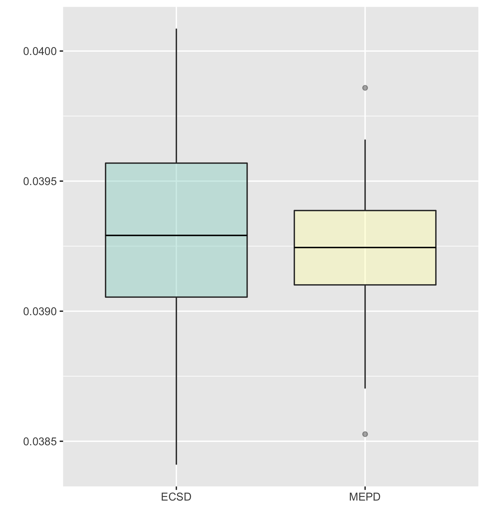
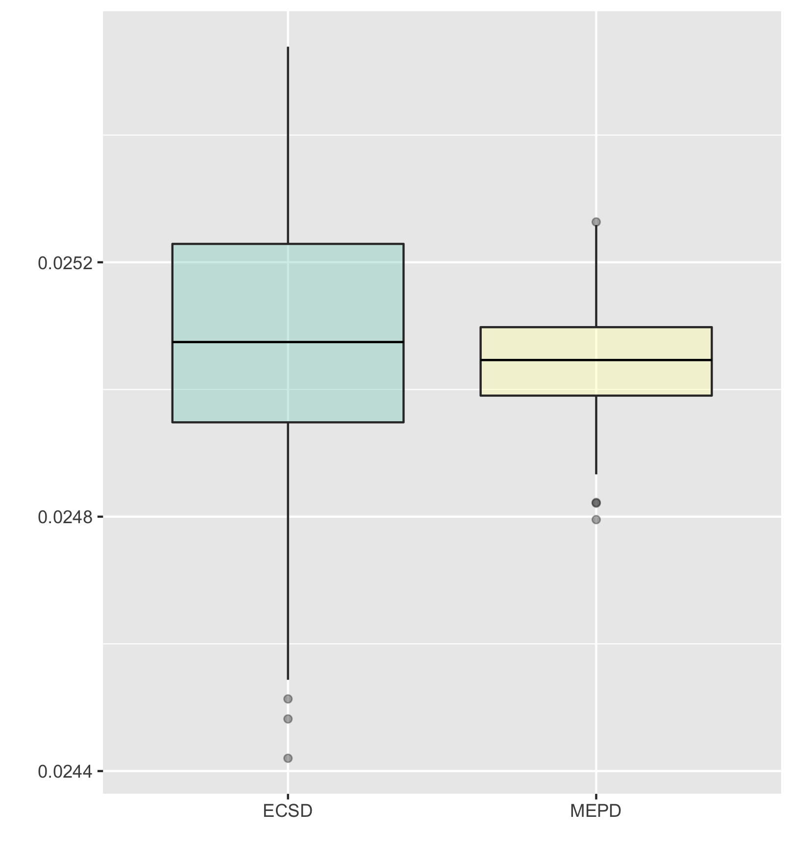
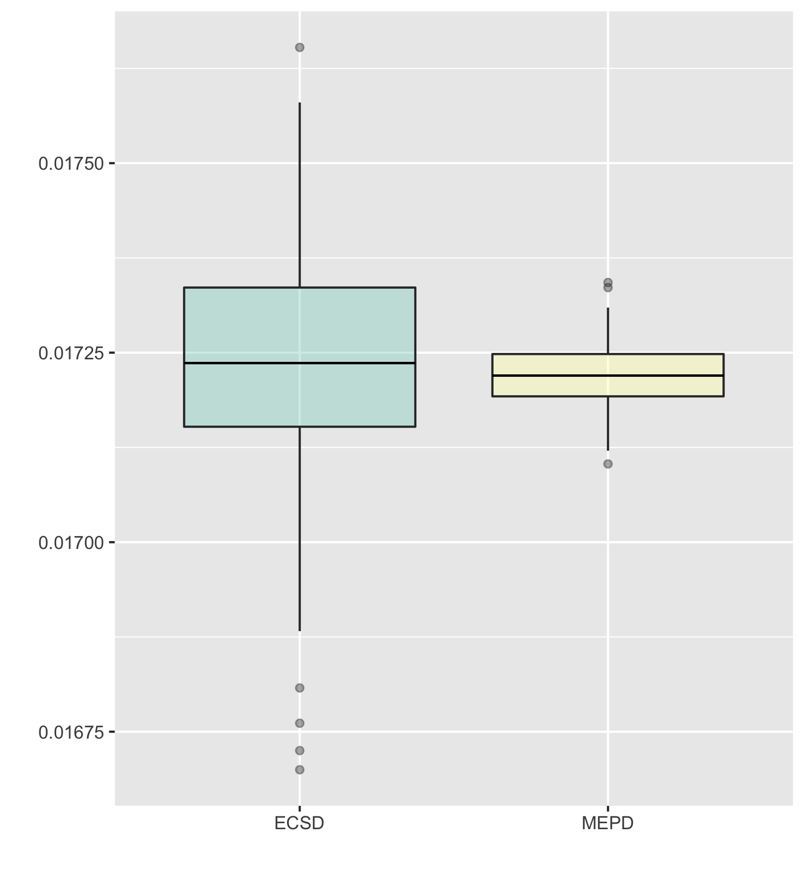
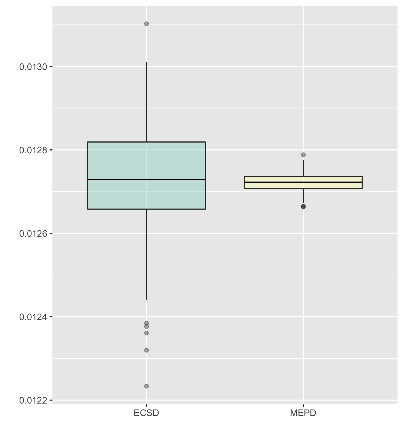
where we remind that $\operatorname{sech}(t)=2/(e^{t}+e^{-t})$. This choice stems from the fact that $\operatorname{sech}$ is an eigenfunction for the Fourier Transform operator. Hence we will compute expectation of similar functions in the both domains, which will make this experiment fair. In Original domain, we estimate $V$ with $\frac{1}{n}\sum_{i=1}^{n}g(X_{i})$, where $X_{1},\ldots,X_{n}$ is an independent sample from $\pi$. Methods to sample from elliptically contoured stable distribution are described in Nolan (2013). In Fourier domain, we use representation (1) and estimate $V$ with $\frac{1}{n}\frac{C_{p}}{(2\pi)^{d}}\sum_{i=1}^{n}\mathcal{F}[g](X_{i})\mathcal{F}[\pi](X_{i})/|\mathcal{F}[\pi](X_{i})|$, where now $X_{1},\ldots,X_{n}$ is an independent sample from $p\propto|\mathcal{F}[\pi]|$, which is called multivariate exponential power distribution. The normalizing constant $C_{p}$ can be computed directly, $C_{p}=\sqrt{2/\alpha}\Gamma(d/\alpha)/(2^{d}\pi^{d/2}\Gamma(d/2)\det(\Sigma))$, where $\Gamma$ stands for the Gamma function.

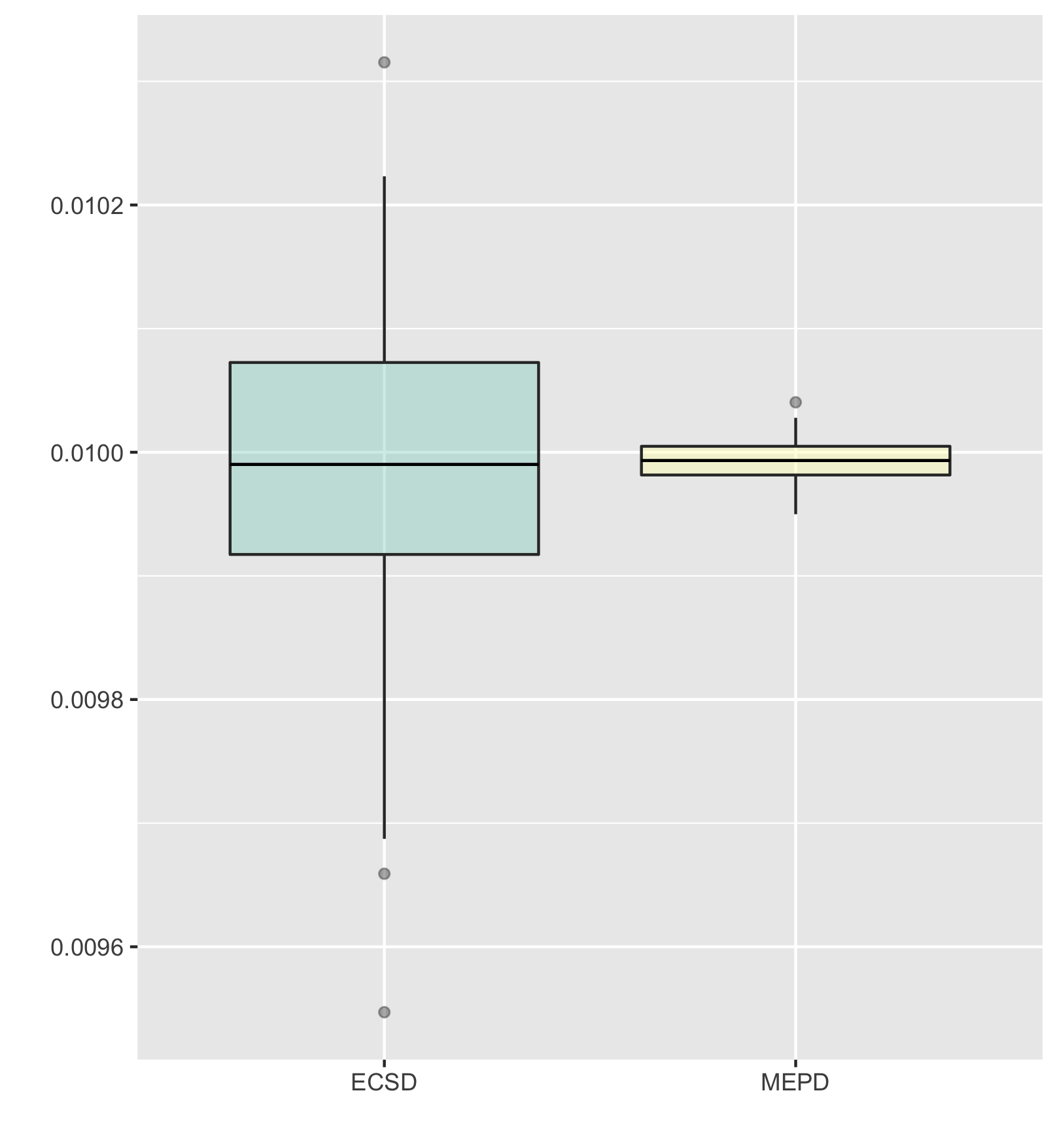
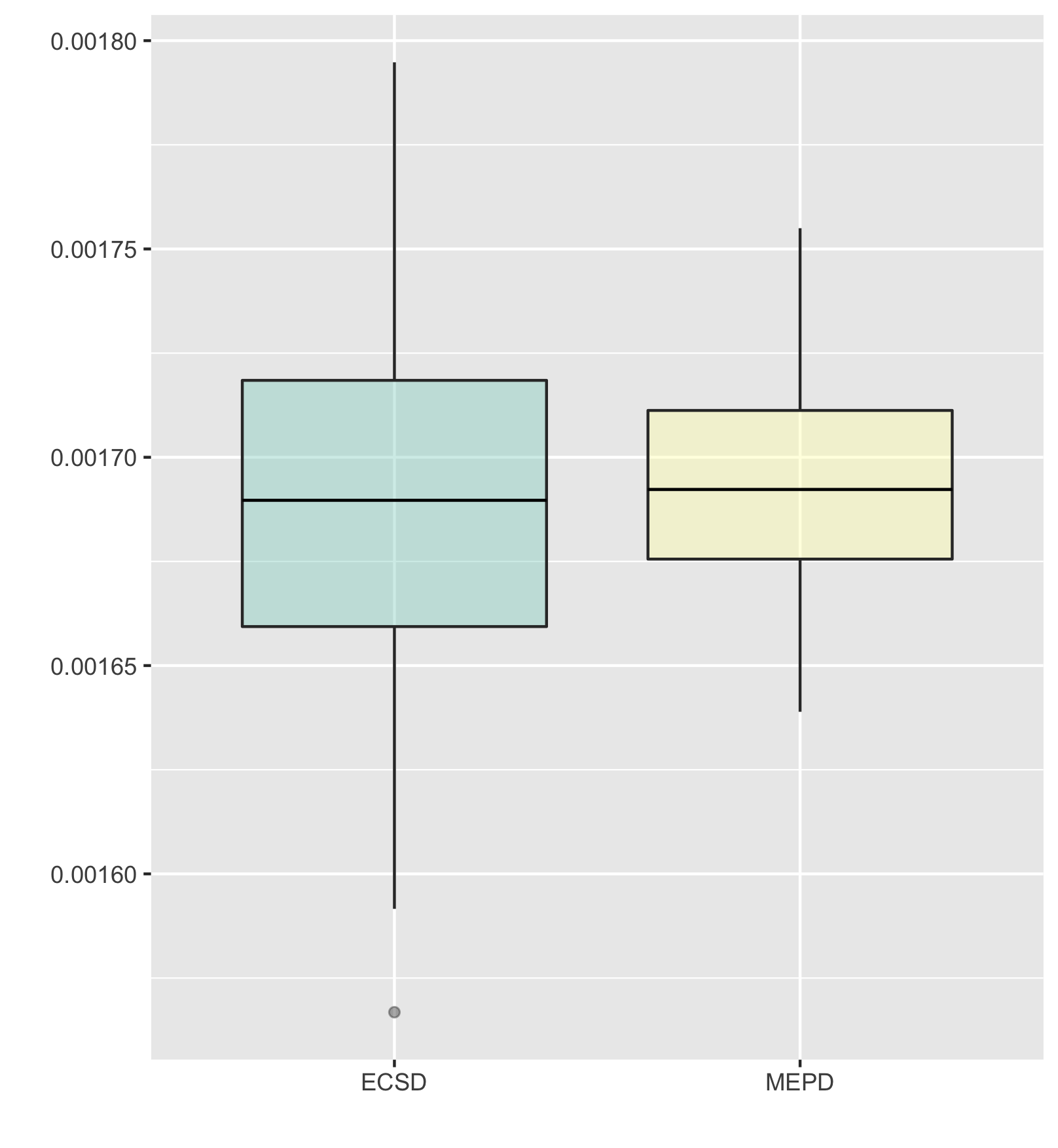
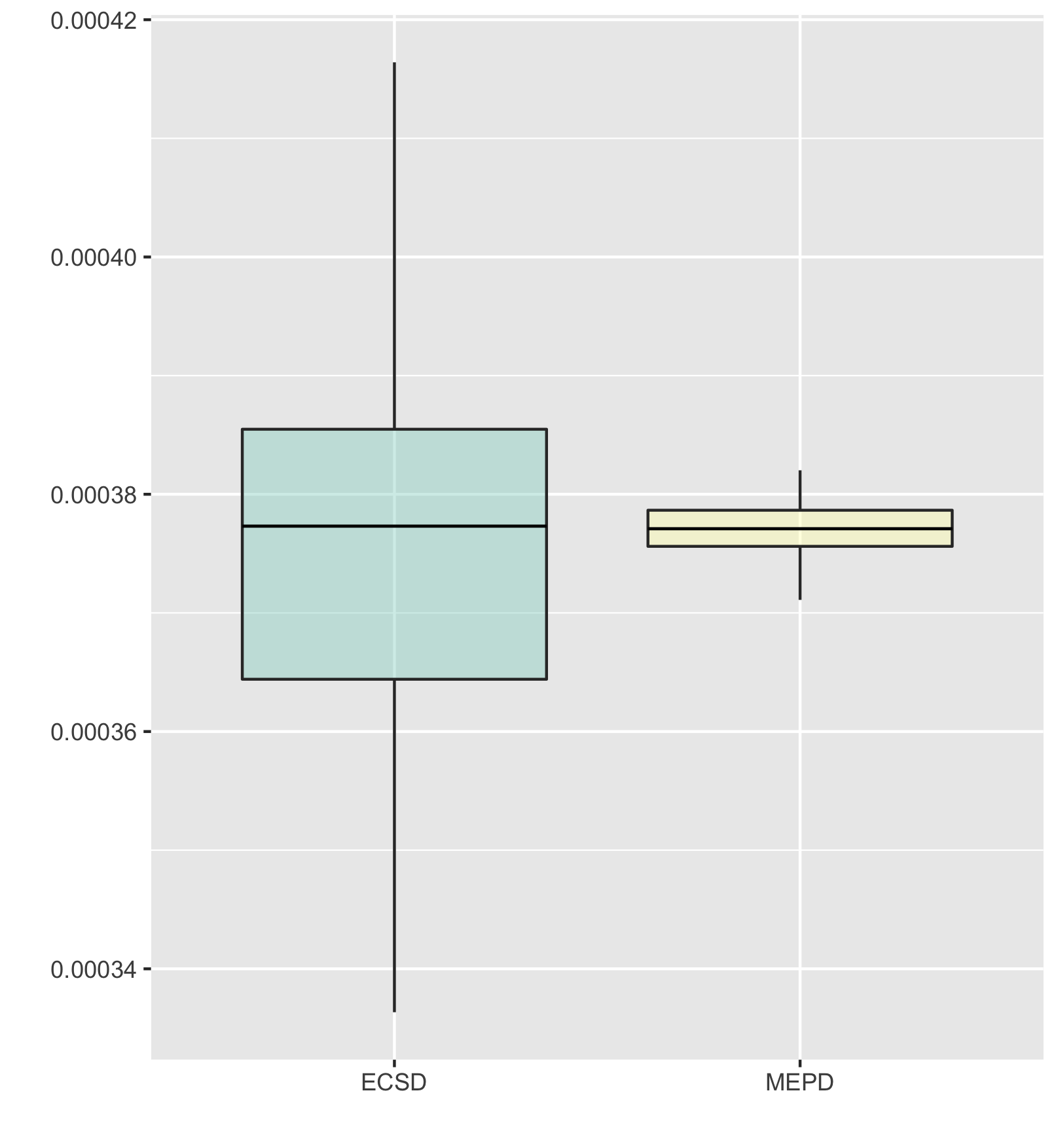
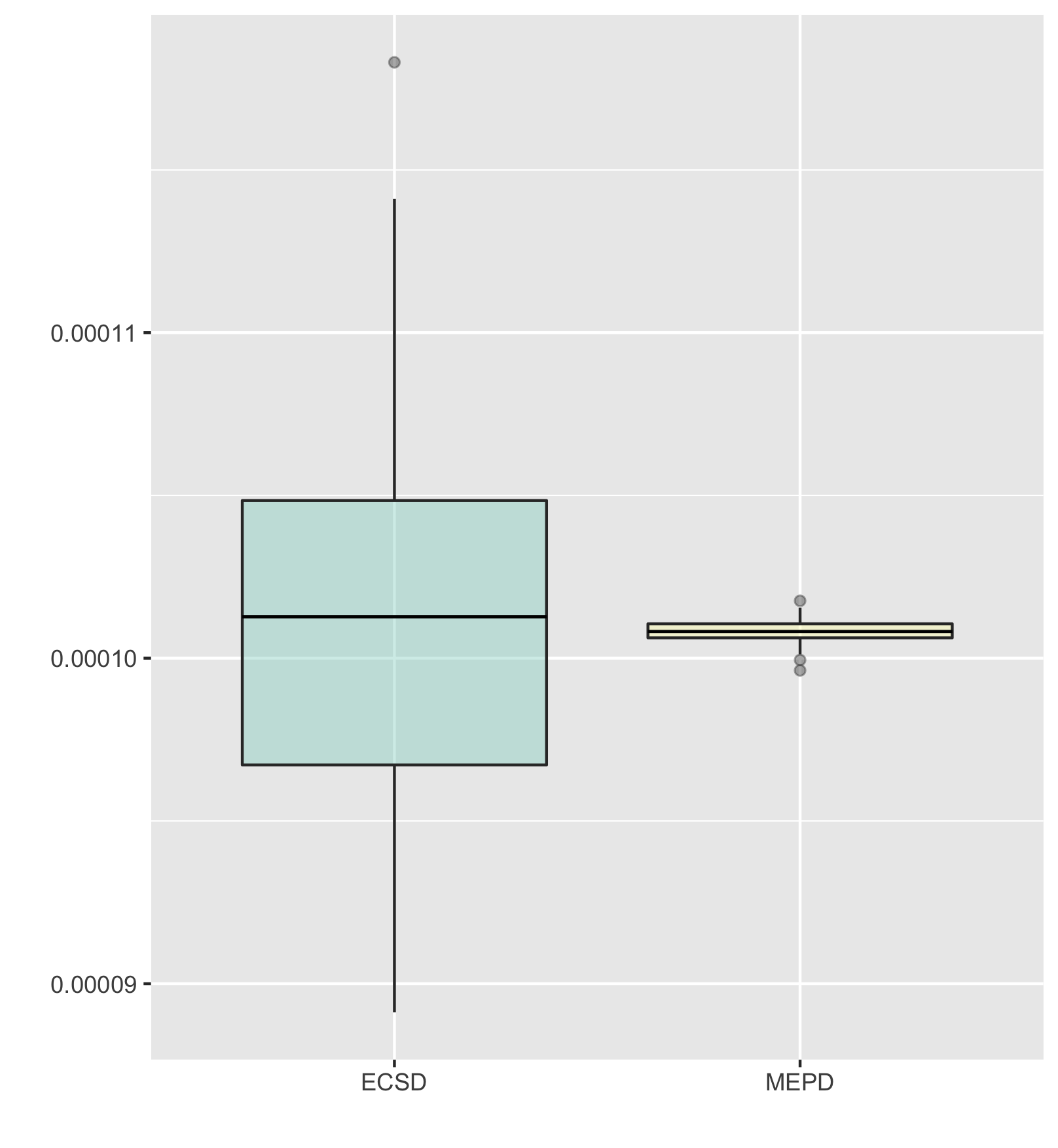
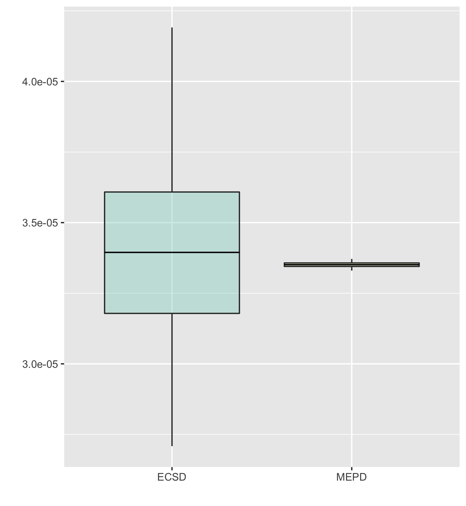
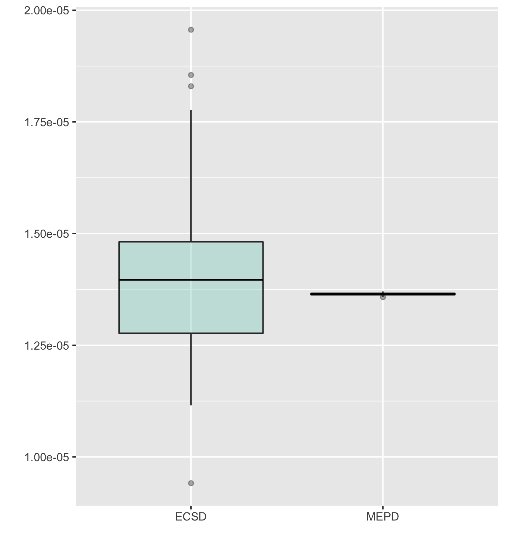
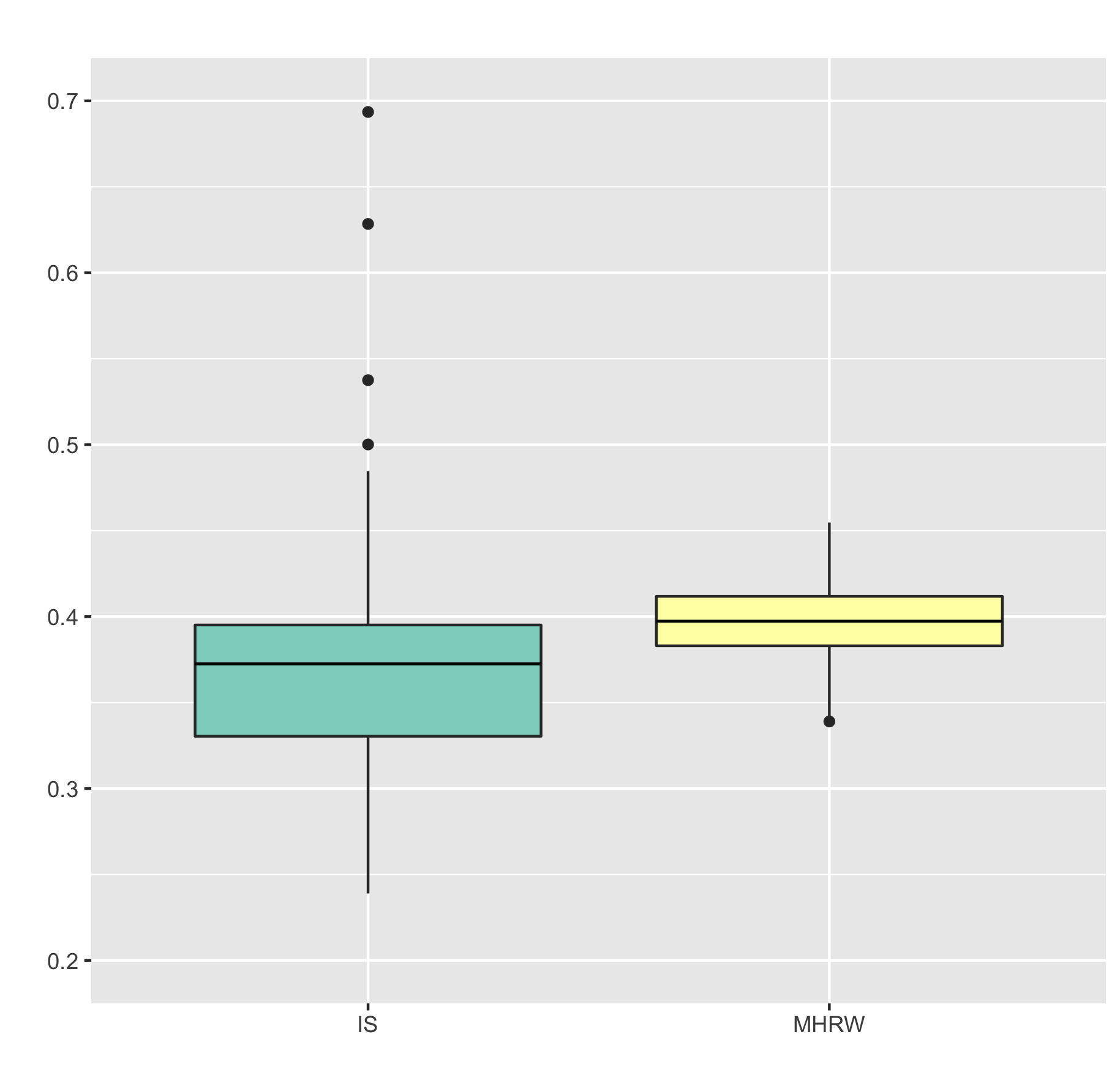
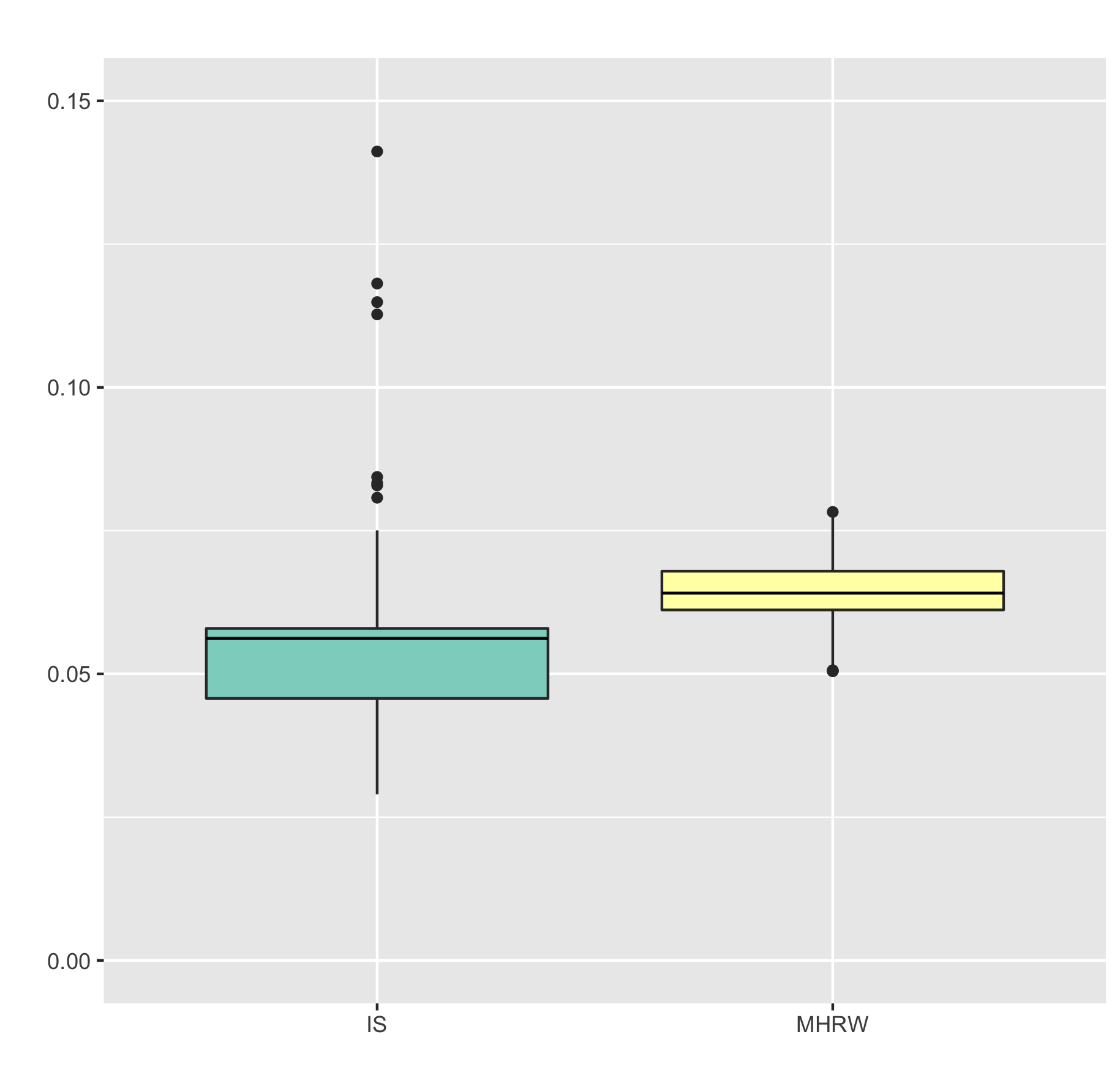
We consider $d=5$ and $d=10$. We let $\mu=0$ and $\Sigma=U^{\top}DU$, where $U$ is a random rotation matrix and $D$ is a diagonal matrix with numbers from $1$ to $d$ on the diagonal. We compute $100$ estimates based on samples of size $n=100\,000$. The spread of this estimates for elliptically contoured stable distribution (ECSD) and multivariate exponential power distribution (MEPD) is given in Figure 1 and Figure 2. We see that the idea of moving to Fourier domain is reasonable — since samples from MEPD have lower variance, we obtain better estimates for $V$.

Figure 1: Monte Carlo estimation of $\mathsf{E}_{\pi}[g]$ in $d=5$ for elliptically contoured stable distribution $\pi$ with $\alpha=1,\,1.2,\,1.4,\,1.6,\,1.8$.

Figure 2: Monte Carlo estimation of $\mathsf{E}_{\pi}[g]$ in $d=10$ for elliptically contoured stable distribution $\pi$ with $\alpha=1,\,1.2,\,1.4,\,1.6,\,1.8$.

5.2 MCMC in Original and Fourier domains

Here we consider a specific case of elliptically contoured stable distributions with $\alpha=1$, the Cauchy distribution. In this case, the density $\pi$ is no longer intractable and is given by

$$\pi(x)=\frac{\Gamma(\frac{d+1}{2})}{\pi^{\frac{d+1}{2}}(\det(\Sigma))^{\frac{1}{2}}}\,\frac{1}{(1+(x-\mu)^{\top}\Sigma^{-1}(x-\mu))^{\frac{d+1}{2}}},$$

where, we recall, $\mu\in\mathbb{R}^{d}$ is a shift vector and $\Sigma$ is a $d\times d$ positive-definite matrix. Its Fourier transform is given by

$$\mathcal{F}[\pi](u)=\exp\left(-(u^{\top}\Sigma u)^{1/2}+iu^{\top}\mu\right).$$

Our aim is still an estimation of $V=\mathsf{E}_{\pi}[g]$ for the same function $g$ given in (6), but now we will use MCMC algorithms. In Original domain, we estimate $V$ with $\frac{1}{n}\sum_{i=1}^{n}g(X_{i})$, where $X_{1},\ldots,X_{n}$ is a Markov chain generated by MALA, MHRW or MHIS algorithms with the target distribution $\pi$. In Fourier domain, we estimate $V$ with $\frac{1}{n}\frac{C_{p}}{(2\pi)^{d}}\sum_{i=1}^{n}\mathcal{F}[g](X_{i})\mathcal{F}[\pi](X_{i})/|\mathcal{F}[\pi](X_{i})|$, see (1), where now $X_{1},\ldots,X_{n}$ is a Markov chain generated by the same MCMC algorithms with the target distribution $p\propto|\mathcal{F}[\pi]|$.

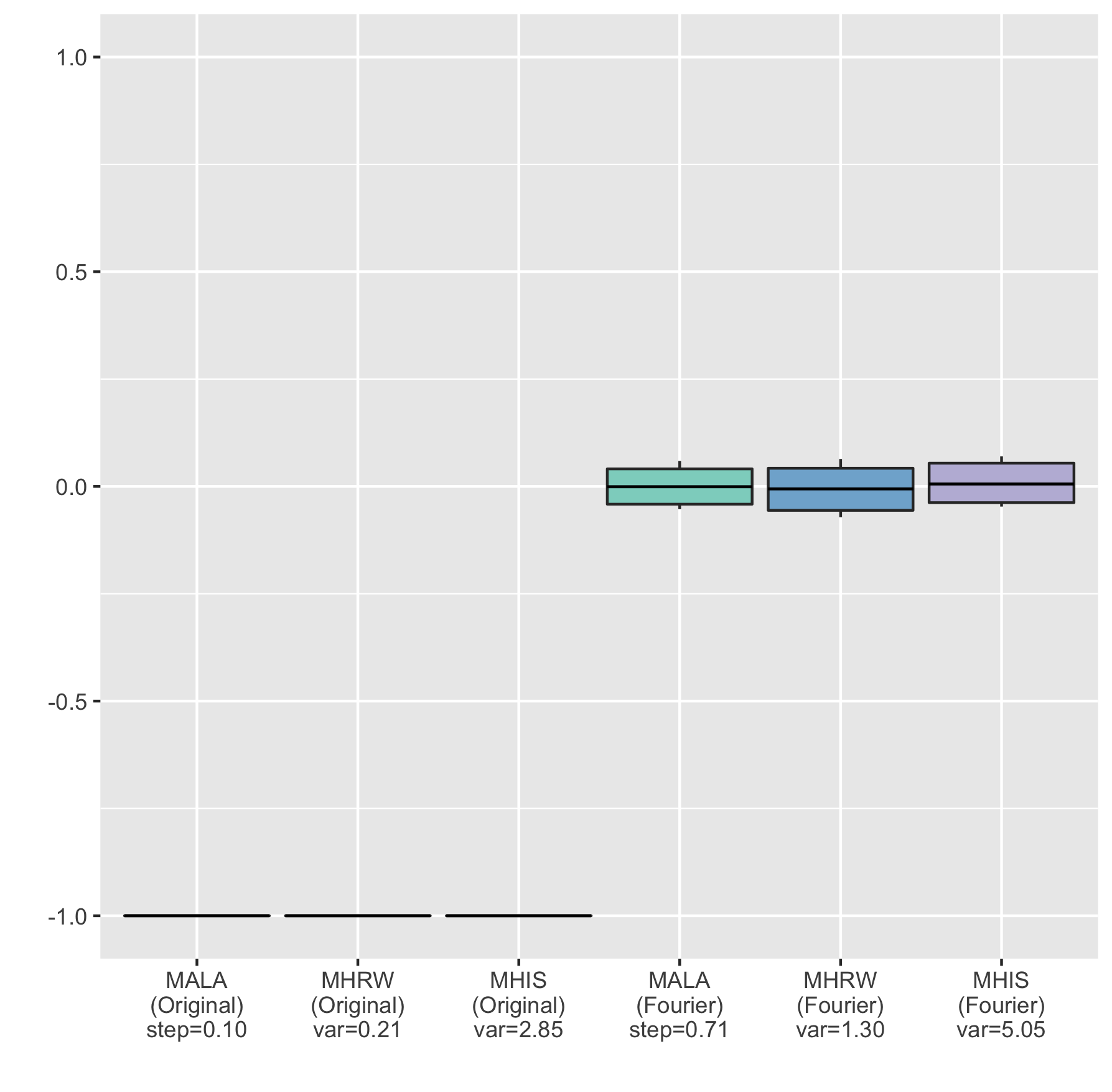
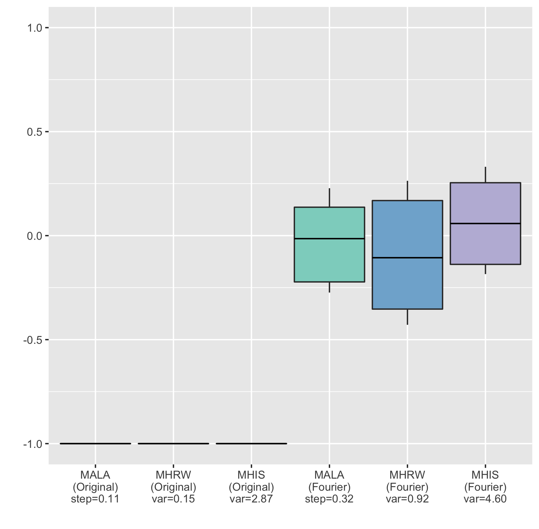
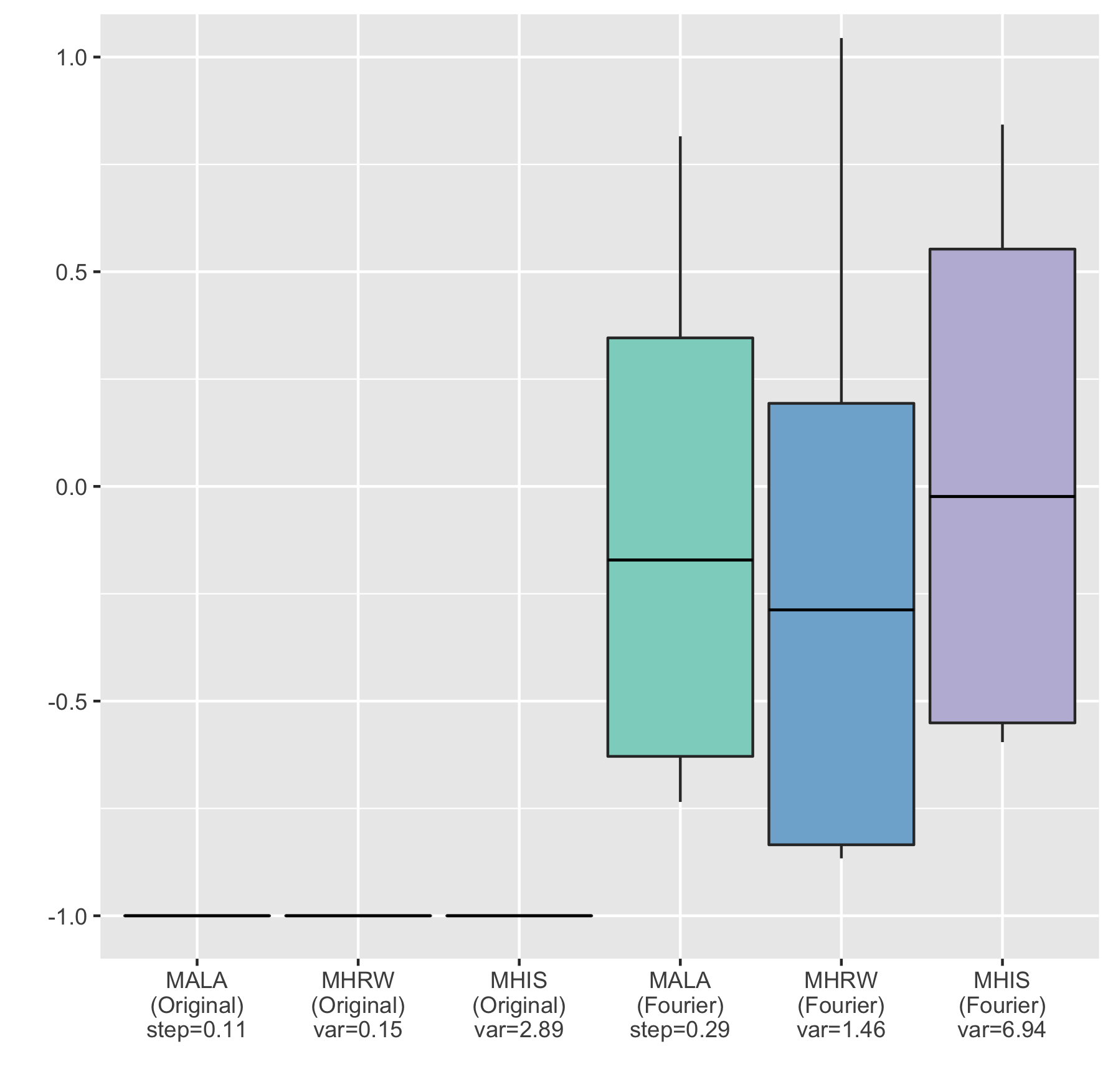
The experiment is organized as follows. We chose $\mu=0$ and $\Sigma=U^{\top}DU$, where $U$ is a random rotation matrix and $D$ is a diagonal matrix with numbers from $0.2$ to $0.2d$ on the diagonal. The matrix $\Sigma$ is chosen so to prevent large values for $C_{p}$. We start with computing of a gold estimate for $V$. This is done by averaging $100$ vanilla Monte Carlo estimates of size $n=100\,000$. For MCMC algorithms, we generate $100$ independent trajectories of size $n=105\,000$, where the first $n=5\,000$ steps are discarded as a burn-in. For both MHRW and MHIS we use the normal proposal. Parameters for MCMC algorithms are chosen adaptively by minimizing the MSE between the gold estimate and $100$ estimates computed for each trajectory. The resulting parameters can be viewed as a best possible parameters, and the performance of an MCMC algorithm as a best possible. Once parameters are estimated, we generate $100$ new independent trajectories of the same size and compute estimates of $V$ for each of them. The relative error of these estimates (with respect to the gold estimate) for $d=5,\,10,\,15$ is shown on boxplots in Fugure 3. We see that MCMC algorithms do not work when the target density has heavy tails, hence moving to Fourier domain might be the only possible option (if, for example, there is no direct sampling algorithm from $\pi$).

Figure 3: MCMC estimation of $\mathsf{E}_{\pi}[g]$ in $d=5,\,10,\,15$ for the Cauchy distribution.

5.3 European Put Option Under CGMY Model

Now we consider a Financial example from Belomestny et al. (2016). The CGMY process $\{X_{t}\}_{r\geq 0}$ is a pure jump process with the Lévy measure

$$\nu_{\text{I}}(x)=C\biggl{[}\frac{e^{Gx}}{|x|^{1+Y}}\mathds{1}_{x<0}+\frac{e^{-Mx}}{|x|^{1+Y}}\mathds{1}_{x>0}\biggl{]},$$

where $C,G,M>0$, $0<Y<2$, see Carr et al. (2002) for details on CGMY processes. The characteristic function of $X_{T}$ reads as

$$\mathcal{F}[\pi](u)=\exp\bigl{(}{i}\mu uT+TC\Gamma(-Y)[(M-iu)^{Y}-M^{Y}+(G+iu)^{Y}-G^{Y}]\bigr{)},$$

where the drift $\mu\in\mathbb{R}^{d}$ is given for some $r>0$ by

$$\mu=r-C\Gamma(-Y)[(M-1)^{Y}-M^{Y}+(G+1)^{Y}-G^{Y}].$$

Suppose that the stock prices follow the model

$$S^{k}_{t}=e^{X^{k}_{t}},\quad k=1,\ldots,d,$$

where $X^{k}_{t}$ are independent CGMY processes. Let $g(x)$ be the payoff function for the put option on the maximum of $d$ assets, i.e.,

$$g(x)=(K-e^{x_{1}}\vee\ldots\vee e^{x_{d}})^{+}.$$

Our goal is to compute the price of the European put option which is given by $V=e^{-rT}\mathsf{E}\bigl{[}g(X^{1}_{T},\ldots,X^{d}_{T})\bigr{]}.$ Application of the Parseval’s formula with damping the growth of $g(x)$ by $e^{\langle x,R\rangle}$ for some vector $R\in\mathbb{R}^{d}$ leads to the formula

$$V=\frac{e^{-rT}}{(2\pi)^{d}}\int_{\mathbb{R}^{d}}\mathcal{F}[g]({i}R-u)\mathcal{F}[\pi](u-{i}R)\,du.$$

To ensure the finiteness of $\mathcal{F}[\pi](u-{i}R)$, we need to choose $R$ such that its coordinates satisfy $-G<R_{k}<0$, $k=1,\ldots,d$. The authors in Belomestny et al. (2016) propose to use importance sampling strategy with the following representation

$$V=\frac{e^{-rT}}{(2\pi)^{d}}\,\mathsf{E}_{X\sim q}\left[\mathcal{F}[g]({i}R-X)\frac{\mathcal{F}[\pi](X-{i}R)}{|q(X)|}\right],\quad\text{where}\quad q(u)=\frac{1}{2\theta^{1/\alpha}\Gamma(1+1/\alpha)}e^{-\frac{|u|^{\alpha}}{\theta}}$$

for some parameters $\alpha,\theta>0$. Our goal is to compare this approach with the Fourier transform MCMC strategy

$$V=\frac{C_{p}e^{-rT}}{(2\pi)^{d}}\,\mathsf{E}_{X\sim p}\left[\mathcal{F}[g]({i}R-X)\frac{\mathcal{F}[\pi](X-{i}R)}{|\mathcal{F}[\pi](X-{i}R)|}\right],$$

where $p(u)\propto|\mathcal{F}[\pi]({i}R-u)|$. The Fourier transform of the payoff function $g(x)$ is given by

$$\mathcal{F}[g]({i}R-u) =\frac{(-1)^{d+1}K^{1-\sum_{k=1}^{d}(R_{k}-{i}u_{k})}}{(\sum_{k=1}^{d}(R_{k}-{i}u_{k})-1)\prod_{k=1}^{d}(R_{k}+{i}u_{k})},$$

see (Eberlein et al., 2010, Appendix A) for the proof.

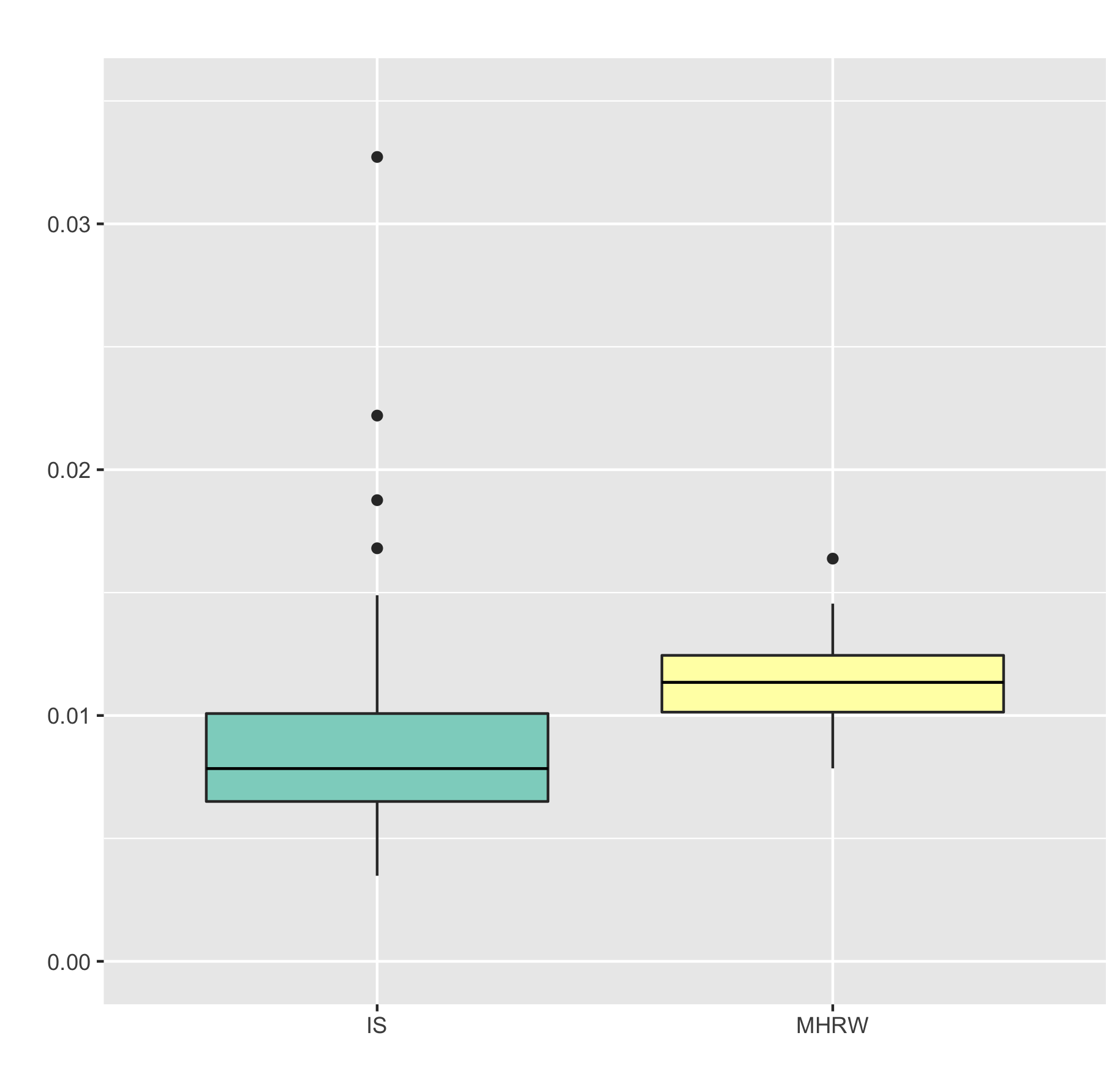
We take $C=1$, $G=5$, $M=5$, $Y=0.5$, $r=0.1$, $S_{0}=100$, $K=100$, $T=1$, $R=-(1.5,\ldots,1.5)$, and compare importance sampling (IS) with Metropolis-Hastings Random Walk (MHRW) by generating $100$ independent trajectories of size $n=10\,000$ and computing estimates of $V$ for each of them. We use the normal density for both importance sampling density (this corresponds to $\alpha=2$, $\theta=2$) and proposal density in MHRW. The burn-in period for MHRW is $N=5\,000$. The spread of the estimates is presented in Figure 4.

Figure 4: Put option on the maximum of $d$ assets in CGMY model for $d=2,4,6$, and $8$.

6 Discussion

We proposed a novel MCMC methodology for the computation of expectation with respect to distributions with analytically known Fourier transforms. The proposed approach is rather general and can be also used in combination with importance sampling as a variance reduction method. As compared to the MC method in spectral domain, our approach requires only generation of simple random variables and therefore is computationally more efficient. Finally let us note that our methodology may also be useful in the case of heavy tailed distributions with analytically known Fourier transforms.

References

- Belomestny et al. (2016) Belomestny, D., Chen, N., Wang, Y., 2016. Unbiased Simulation of Distributions with Explicitly Known Integral Transforms. Monte Carlo and Quasi-Monte Carlo Methods. Springer Proceedings in Mathematics & Statistics 163, 229–244.
- Belomestny et al. (2015) Belomestny, D., Comte, F., Genon-Catalot, V., Masuda, H., Reiß, M., 2015. Lévy matters. IV. Vol. 2128 of Lecture Notes in Mathematics. Springer, Cham, estimation for discretely observed Lévy processes, Lévy Matters.
- Brosse et al. (2018a) Brosse, N., Durmus, A., Meyn, S., Moulines, E., 2018a. Diffusion approximations and control variates for MCMC. arXiv preprint arXiv:1808.01665.
- Brosse et al. (2018b) Brosse, N., Durmus, A., Moulines, É., et al., 2018b. Normalizing constants of log-concave densities. Electronic Journal of Statistics 12 (1), 851–889.
- Carr et al. (2002) Carr, P., Geman, H., Madan, D. B., Yor, M., 2002. The fine structure of asset returns: an empirical investigation. J. Bus. 75 (2), 305–333.
- Dalalyan (2017) Dalalyan, A. S., 2017. Theoretical Guarantees for Approximate Sampling from Smooth and Log‐concave Densities. J. R. Stat. Soc. B 79 (3), 651–676.
- Dedecker and Gouëzel (2015) Dedecker, J., Gouëzel, S., 2015. Subgaussian concentration inequalities for geometrically ergodic Markov chains. Electron. Commun. Probab. 20 (64).
- Durmus and Moulines (2017) Durmus, A., Moulines, E., 2017. Nonasymptotic Convergence Analysis for the Unadjusted Langevin Algorithm. Ann. Appl. Probab. 27 (3), 1551–1587.
- Eberlein et al. (2010) Eberlein, E., Glau, K., Papapantoleon, A., 2010. Analysis of Fourier Transform Valuation Formulas and Applications. Applied Mathematical Finance 17 (3), 211–240.
- Gamerman and Lopes (2006) Gamerman, D., Lopes, H. F., 2006. Markov chain Monte Carlo, 2nd Edition. Texts in Statistical Science Series. Chapman & Hall/CRC, Boca Raton, FL, stochastic simulation for Bayesian inference.
-
Glasserman and Liu (2010)
Glasserman, P., Liu, Z., 2010. Sensitivity estimates from characteristic
functions. Oper. Res. 58 (6), 1611–1623.
URL https://doi.org/10.1287/opre.1100.0837 - Hastings (1970) Hastings, W. K., 1970. Monte Carlo sampling methods using Markov chains and their Applications. Biometrika 57, 97–109.
- Havet et al. (2019) Havet, A., Lerasle, M., Moulines, E., Vernet, E., 2019. A quantitative Mc Diarmid’s inequality for geometrically ergodic Markov chains. arXiv preprint arXiv:1907.02809.
- Ibragimov and Linnik (1971) Ibragimov, I. A., Linnik, Y. V., 1971. Independent and Stationary Sequences of Random Variables. Walters-Noordhoff, The Netherlands.
Jarner and Hansen (2000)
Jarner, S. F., Hansen, E., 2000. Geometric ergodicity of Metropolis
algorithms. Stochastic Processes and their Applications 85 (2), 341 – 361.
URL http://www.sciencedirect.com/science/article/pii/S0304414999000824 - Jarner and Tweedie (2003) Jarner, S. F., Tweedie, R. L., 2003. Necessary Conditions for Geometric and Polynomial Ergodicity of Random-Walk-Type Markov Chains. Bernoulli 9 (4), 559–578.
- Jones (2004) Jones, G. L., 2004. On the Markov chain central limit theorem. Probability Surveys 1, 299–320.
Kendall et al. (2005)
Kendall, W. S., Liang, F., Wang, J.-S. (Eds.), 2005. Markov chain Monte
Carlo. Vol. 7 of Lecture Notes Series. Institute for Mathematical Sciences.
National University of Singapore. World Scientific Publishing Co. Pte. Ltd.,
Hackensack, NJ, innovations and applications.
URL https://doi.org/10.1142/9789812700919 - Mengersen and Tweedie (1996) Mengersen, K. L., Tweedie, R. L., 1996. Rates of convergence of the Hastings and Metropolis algorithms. The Annals of Statistics 24 (1), 101–121.
- Metropolis et al. (1953) Metropolis, N., Rosenbluth, A. W., Rosenbluth, M. N., Teller, A. H., Teller, E., 1953. Equation of state calculations by fast computing machines. The journal of chemical physics 21 (6), 1087–1092.
- Meyn and Tweedie (1993) Meyn, S. P., Tweedie, R. L., 1993. Markov chains and stochastic stability. New York: Springer-Verlag.
Müller-Gronbach et al. (2012)
Müller-Gronbach, T., Novak, E., Ritter, K., 2012. Monte
Carlo-Algorithmen. Springer-Lehrbuch. Springer, Heidelberg.
URL https://doi.org/10.1007/978-3-540-89141-3 - Nolan (2013) Nolan, J. P., 2013. Multivariate Elliptically Contoured Stable Distributions: Theory and Estimation. Comput. Stat. 28 (5), 2067–2089.
- Nolan (2018) Nolan, J. P., 2018. Stable Distributions - Models for Heavy Tailed Data. Birkhauser, Boston, in progress.
- Roberts and Tweedie (1996) Roberts, G., Tweedie, R., 1996. Geometric convergence and central limit theorems for multidimensional Hastings and Metropolis algorithms. Biometrika 83, 95–110.
- Sato (1999) Sato, K.-I., 1999. Lévy Processes and Infinitely Divisible Distributions. Cambridge University Press.
- Tankov (2003) Tankov, P., 2003. Financial modelling with jump processes. Vol. 2. CRC press.
- Tierney (1994) Tierney, L., 1994. Markov chains for exploring posterior distributions. The Annals of Statistics 22 (4), 1701–1762.
- Wintenberger (2017) Wintenberger, O., 2017. Exponential inequalities for unbounded functions of geometrically ergodic Markov chains: applications to quantitative error bounds for regenerative Metropolis algorithms. Statistics 51 (1), 222–234.