How much joint resummation do we need?
Abstract
Large logarithms that arise in cross sections due to the collinear and soft singularities of QCD are traditionally treated using parton showers or analytic resummation. Parton showers provide a fully-differential description of an event but are challenging to extend beyond leading logarithmic accuracy. On the other hand, resummation calculations can achieve higher logarithmic accuracy but often for only a single observable. Recently, there have been many resummation calculations that jointly resum multiple logarithms. Here we investigate the benefits and limitations of joint resummation in a case study, focussing on the family of event shapes called angularities. We calculate the cross section differential in angularities at next-to-leading logarithmic accuracy. We investigate whether reweighing a flat phase-space generator to this resummed prediction, or the corresponding distributions from Herwig and Pythia, leads to improved predictions for other angularities. We find an order of magnitude improvement for over , highlighting the benefit of joint resummation, but diminishing returns for larger values of .
1 Introduction
Measurements at colliders often impose restrictions on QCD radiation through e.g. jet vetoes, transverse momentum measurements, or production at threshold. One particular example, that will play a prominent role in this paper, is the family of event shapes for collisions called angularities Berger:2003iw . These are defined as
| (1) |
where is the center-of-mass energy, and the sum runs over all final-state particles with energy and angle with respect to a chosen axis. The cross section integrated over up to some cut-off , known as the cumulative cross section, contains a series of logarithms at each order in perturbation theory, schematically
| LO | |||||
| NLO | |||||
| NNLO | |||||
| LLNLLNNLL | (2) | ||||
Rows correspond to different orders of fixed-order perturbation theory, denoted by leading order (LO), next-to-leading order (NLO), etc. For , the expansion breaks down, because we cannot treat . In this case we want to sum columns, which correspond to different orders of resummed perturbation theory, called leading logarithmic (LL) order, next-to-leading logarithmic (NLL) order, etc. To be precise, we will treat , which corresponds to resumming logarithms “in the exponent”.
This resummation can be carried out either by using a Monte Carlo parton shower, such as Herwig Bahr:2008pv ; Bellm:2015jjp ; Bellm:2017bvx or Pythia Sjostrand:2014zea , or through analytical methods. The advantage of parton showers is that they allow for any measurement on the fully exclusive final state. However, their formal accuracy is limited to LL order in the large limit, and it is challenging to systematically go beyond this order. For a recent discussion of the logarithmic accuracy of the parton shower, see refs. Hoeche:2017jsi ; Dasgupta:2018nvj ; Bewick:2019rbu . Some recent improvements in parton showers are the inclusion of higher-order splitting functions Jadach:2016zgk ; Li:2016yez ; Hoche:2017iem ; Hoche:2017hno , corrections to the large limit Nagy:2015hwa ; Isaacson:2018zdi ; Platzer:2018pmd , spin correlations Richardson:2018pvo , and the simultaneous treatment of small and collinear and soft logarithms Andersen:2017sht .
On the other hand, analytic resummation calculations are able to achieve a much higher precision. As an example, in the case of angularities, predictions at NNLL+NNLO accuracy are available Banfi:2018mcq ; Bell:2018gce . Methods for analytic resummation include the CSS formalism Collins:1985ue ; Collins:1988ig ; Collins:1989gx , those based on the coherent-branching formalism Banfi:2001bz ; Banfi:2004yd ; Banfi:2014sua , and those using renormalization group evolution in effective field theories of QCD, such as Soft-Collinear Effective Theory (SCET) Bauer:2000ew ; Bauer:2000yr ; Bauer:2001ct ; Bauer:2001yt . While many of these calculations have focussed on the resummation of a single logarithmic series, there has recently been a significant effort to jointly resum multiple logarithms. This includes the joint resummation of logarithms due to threshold production and transverse momentum Li:1998is ; Laenen:2000ij ; Kulesza:2002rh ; Kulesza:2003wn ; Lustermans:2016nvk ; Marzani:2016smx ; Muselli:2017bad , threshold and small Ball:2013bra ; Bonvini:2018ixe , transverse momentum and small Marzani:2015oyb , transverse momentum and beam thrust Procura:2014cba ; Lustermans:2019plv , jet mass and dijet invariant mass Bauer:2011uc ; Pietrulewicz:2016nwo , two angularities Larkoski:2014tva ; Procura:2018zpn , jet veto and jet radius Banfi:2015pju , jet mass and jet radius Kolodrubetz:2016dzb , jet vetoes and jet rapidity Hornig:2017pud ; Michel:2018hui , and threshold and jet radius Liu:2017pbb ; Liu:2018ktv .
In principle, one could imagine the simultaneous resummation of ever more observables, which would lead to an increasingly precise parton shower. This is important for the burgeoning field of Machine Learning in jet substructure, see ref. Larkoski:2017jix for a review. Here, samples from Monte Carlo parton showers are often employed, thus raising the question to what extent discrimination is based on features of physics or of the Monte Carlo. There has also been some work on approaches that do not require labeled samples though, see e.g. refs. Metodiev:2017vrx ; Cohen:2017exh ; Metodiev:2018ftz ; Andreassen:2018apy . We were inspired by ref. Datta:2017rhs , which investigates how sensitive Machine Learning is to details of the final state, studying the discrimination of jets from boosted, hadronic decays of bosons from jets initiated by QCD processes. By using a complete basis of observables that probe the -body final state and increasing , they find that the discrimination saturates at .
We are interested in asking how much resummation is needed to reliably describe the jet, focussing on QCD-initiated jets. For simplicity, we restrict ourselves to observables that are azimuthally symmetric, for which the angularities form a basis. Specifically, we consider a set of angularities , with , derive the resummed prediction for the cross section differential in a subset of angularities denoted by at NLL accuracy, and investigate the degree to which any of the other angularities , with , can be predicted. To this end, we generate events from flat111“Flat” here implies that there are no preferred points in phase space, so that, up to four-momentum conservation, each point is assigned the same probability. -body phase space, using Rambo Kleiss:1985gy “on diet” Platzer:2013esa . We reweigh these events to match the multi-differential cross sections from the input, and then calculate the distributions for other angularities from these reweighed events. As an alternative to analytic resummation, we also use the cross section differential in angularities from Herwig or Pythia as basis for reweighing. The dependence of this procedure on the number of angularities that have been jointly resummed is investigated and the optimal subset of angularities to be used as input for any given is determined.
Our main conclusion is that there is an order of magnitude improvement for reweighing with angularities over , but that the advantage quickly diminishes for larger values of . We have investigated the dependence on the input (Herwig, Pythia, analytic), number of particles of the flat phase space, center-of-mass energy , and set of angularities under consideration. None of these lead to a qualitatively different behavior.
The outline of this paper is as follows: We start in sec. 2 by describing our setup and discussing in detail how we perform the reweighing, determine the optimal input set of angularities , and estimate the statistical uncertainty. In sec. 3, we present our analytic calculation of the cross section differential in angularities, limiting most of the discussion to NLL accuracy. Our main results are presented in sec. 4, with additional plots relegated to app. A. We conclude in sec. 5.
2 Optimal reweighing procedure
We start this section by presenting our setup, discussing the observables in more detail. We then describe the reweighing procedure of flat -body phase space with resummed predictions for angularities, as well as the determination of the optimal set of angularities to be used as input, including the treatment of statistical uncertainties.
2.1 Setup
We use the process as a case-study for our procedure. The final state of the collision is clustered into two jets using the exclusive Catani:1991hj jet algorithm with the Winner-Take-All (WTA) recombination scheme Salam:WTAUnpublished ; Bertolini:2013iqa . Following ref. Larkoski:2014uqa , we modify the original definition of the angularities in ref. Berger:2003iw for large angles , as described by eq. (1). The angle of each particle contributing to an angularity is measured with respect to the WTA axis of the corresponding jet, and the angularities that we consider are the sum of the angularities of the individual jets, i.e. . The variable is used instead of the angularities themselves, which is more natural since the angularity distributions are peaked at small values of .222For brevity, we will also refer to the observables as “angularities”.
The various distributions of are constructed in 16 bins on the interval . We have verified that the chosen binning does not alter the conclusions of our study. The binned distributions are constructed either by using analytic predictions (described in sec. 3) or through parton-level events generated by the Herwig 7 or Pythia 8 general-purpose Monte Carlos (described in sec. 2.2).
2.2 Optimal reweighing
To obtain the binned distributions for flat massless -body phase space,
| (3) |
with in the center-of-mass frame, we employ the Rambo technique of refs. Kleiss:1985gy ; Platzer:2013esa , with a slight modification that improves sampling in the collinear and soft regions through weighted events. In particular, we perform a transformation that distributes the first random number of “Algorithm 1” in ref. Platzer:2013esa logarithmically, with the weight of this event given by the Jacobian. This ensures that the phase space is sampled sufficiently to obtain statistically reliable predictions for small values of the angularities that we consider.
We start by reweighing the flat phase space result for angularities by the cross section differential in angularities with . By integration333In our case, the integration is approximated by a sum over bins. over the angularities , a reweighed cross section differential in the remaining angularity with is determined, i.e.
| (4) |
appropriately applied to the binned distributions. Comparisons between the resulting reweighed cross sections and direct determinations of equivalent cross sections can be found in figs. 5 and 6.
We define a goodness-of-fit measure for the reweighed angularity distribution by comparing to the resummed distribution for
| (5) |
To find the optimal set when reweighing with angularities, we introduce a global goodness-of-fit variable, defined as the average of the angularities ,
| (6) |
Here is the number of angularities not used as input.
Up to , we search for the global minimum of as a function of the set of reweighed angularities , denoted by . We will refer to this as the optimal set of angularities in each case, and the corresponding value for will be denoted by . For and , we start from the optimal for angularities and iteratively determine the optimal additional angularity to add to . We have verified that the result of this iterative method is already very close to the global minimum of for .
The value of the global minimum is rather sensitive to statistical fluctuations, owing to the finite size of the Monte Carlo samples distributed over bins.444The -dimensional distributions are required to perform the projection in eq. (4). Furthermore, it is not expected to follow a Gaussian distribution. To obtain an estimate of the statistical uncertainty, we perform the reweighing procedure over 11 replicas of the event samples. The median of is taken as our central prediction, and the spread of the 7 most central replicas as a reasonable approximation for the spread corresponding to roughly one standard deviation. Results for as a function of are depicted in fig. 7 and in app. A.1.
3 Joint resummation of angularities at NLL
In this section we present our framework for performing the joint resummation of angularities. We start by drawing the Lund planes in sec. 3.1, from which the leading-logarithmic resummation immediately follows. These diagrams also allow us to identify the modes in SCET, for which the factorization formulae are presented in sec. 3.2. From the renormalization group equations for these factorization formulae we obtain the resummed cross section at NLL accuracy in sec. 3.3. We describe the matching of the different factorization formulae for different regions of phase space in sec. 3.5, for which we are guided by the size of the power corrections, estimated in sec. 3.4.
3.1 Lund diagrams and phase-space boundaries
In the collinear limit, the probability of a particle emitting real radiation can be characterized by the momentum fraction and angle of the radiated particle with respect to its emitter ,
| (7) |
At LL accuracy, only the term of the splitting function is kept, so these emissions are uniformly distributed in and . The Lund plane Andersson:1988gp spanned by these variables is shown in fig. 1, with some emissions indicated by crosses.
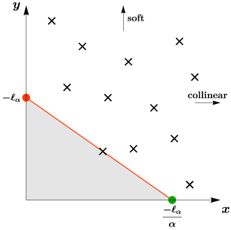
By identifying and (the factor of is purely for convenience and doesn’t affect the leading logarithms), the angularity in eq. (1) for a single emission with small and can be written as
| (8) |
corresponding to a straight line in the Lund plane with slope . Due to their uniform distribution in the (logarithmically-spaced) Lund plane, a single emission will dominate the measurement at this accuracy, as indicated by the red line in fig. 1. All emissions above and to the right of this line are more soft or collinear and only enter beyond LL accuracy. There are no emissions below the line, otherwise these would be dominant. The shaded area under the line corresponds to the Sudakov factor describing the no-emission probability, and can be used to calculate the cumulative cross section,
| (9) |
where is the Born cross section and () for quark (gluon) jets. Interestingly, the relevant degrees of freedom in SCET correspond to the points that describe the edges of the shaded region. For the measurement of a single angularity these are indicated by the orange and green dot in fig. 1, and correspond to soft and collinear modes respectively. The parametric scaling of the momenta of these modes is most conveniently expressed in terms of lightcone coordinates defined through
| (10) |
Indicating the momenta of the soft, -collinear and -collinear modes by , and respectively, their scaling is found to be Hornig:2009vb
| (11) |
When the simultaneous measurement of two angularities and is considered, the straight lines describing the variables in the Lund plane have to cross one another at some point to ensure that the cross section depends on both measurements. Assuming the hierarchy for definiteness, three distinct cases can be distinguished, as shown in fig. 2.
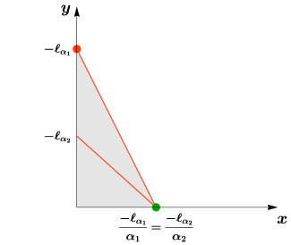
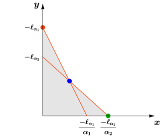
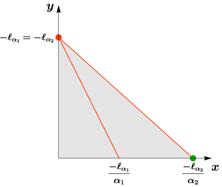
The boundaries of these three regions of phase space for two angularities are
| (12) |
which agree with the regions of phase space identified in refs. Larkoski:2014tva ; Procura:2014cba ; Procura:2018zpn . In all three cases there are soft (orange) and collinear (green) degrees of freedom. The intermediate regime 2 has an additional collinear-soft mode (blue), which contributes to both measurements since it lies on the intersection of both lines.
This method of finding all relevant regions of phase space can be generalized to the simultaneous measurement of an arbitrary number of angularities. There is only one additional subtlety that has to be taken into account when more than two angularities are considered, which we illustrate in fig. 3 for three angularities with parameters . If the line corresponding to were to be placed above the position indicated by the dotted line, the angularity would no longer be connected to the boundary of the region in which emissions are forbidden and hence not affect the cross section. The point at which the dotted line crosses the -axis is given by
| (13) |
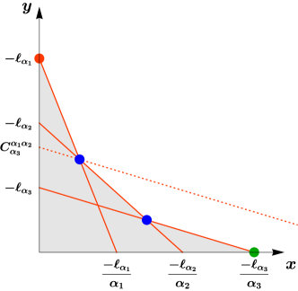
The phase space of a cross section involving an arbitrary number of angularities can be divided into various regimes, as listed explicitly in eq. (3.1) for . The regime in which the largest number of independent logarithms occur, is the one for which the edge of the forbidden (gray) region in the Lund plane involves every line corresponding to an individual angularity. For , this corresponds to the center panel in fig. 2 and for , this situation is depicted in fig. 3. This region will be denoted by , and its boundaries in phase space are given by
| (14) |
The first line consists of the conditions on the hierarchy between the points at which each line in the Lund plane crosses the -axis. The second line contains the conditions on the hierarchy between the points at which the lines cross the -axis. As the conditions consist solely of inequalities, this region in phase space is -dimensional and will be called the “bulk”.
Regions that involve fewer logarithms can be obtained by raising or lowering the point where an angularity crosses either axis in the Lund plane, such that two modes (the colored dots) overlap. This can be seen explicitly in fig. 2 by starting from the center panel and raising until it reaches in the right panel, sliding the mode indicated by the blue dot up to the orange dot in the process. In full generality, the boundaries of a region in phase space involving a subset of angularities with and are found to be555Note that subsequent and do not necessarily correspond to consecutive , although we still adhere to the convention .
| (15) | ||||||
where the -conditions (boundary-conditions) contain all restrictions on the angularities that are only connected to the boundary of the shaded area in the Lund plane through a single point, i.e. the angularities not involved in the region. As any such regime is characterized by equalities, it represents an -dimensional region in the -dimensional phase space, denoted by . By considering all possible combinations of angularities it then follows that there are distinct regions of dimension in the phase space of angularities.
3.2 Factorization formulas
The analytical resummation will be performed by making use of the Soft-Collinear Effective Theory (SCET) Bauer:2000ew ; Bauer:2000yr ; Bauer:2001ct ; Bauer:2001yt , which describes the infrared limit of QCD. The relevant degrees of freedom are determined by the process and measurements under consideration. The version of SCET that involves the collinear and soft modes in eq. (3.1), known as SCET, correctly describes the regions of phase space dominated by a single angularity, e.g. the left and right panels in fig. 2. Regions of phase space involving multiple angularities (such as the middle panel in fig. 2) contain additional collinear-soft modes and are correctly described by SCET+ Procura:2014cba ; Bauer:2011uc ; Larkoski:2015zka ; Pietrulewicz:2016nwo .
As the various modes in SCET are decoupled at the level of the Lagrangian Bauer:2001yt , cross sections may be factorized into products or convolutions of perturbative functions as long as the contributions of the various modes to the measurements can be shown to factorize as well. In general, each of these functions contains logarithms of the ratio of its inherent, natural scale and the common scale . By solving their RGEs, they may be evaluated at their natural scales (where the logarithms are minimized) and then evolved towards a common scale , resumming all the large logarithms in the process.
The relevant degrees of freedom for the bulk regime for angularities are shown in the middle panel of fig. 2. The orange dot represents the (ultra)soft mode, the green dot the collinear mode, and the blue dot corresponds to a collinear-soft mode Bauer:2011uc ; Procura:2014cba , which contributes to the measurement of both angularities. For our process of interest, , there are two distinct collinear directions corresponding to the two jets, and hence also two corresponding collinear and collinear-soft modes. The factorization formula for this regime was derived using SCET in refs. Procura:2014cba ; Procura:2018zpn and reads
| (16) | ||||
where we have defined convolutions between two functions and through
| (17) |
Here the dots represent possible additional arguments. Furthermore, the short-hand notations
| (18) |
are employed, where indicates a convolution in both and . In eq. (16), the hard function contains the Born cross section and virtual corrections to the hard scattering. The jet function describes collinear radiation, the soft function encodes the contribution from soft radiation, and is the collinear-soft function.
The region of phase space represented by the left panel of fig. 2 is reached through raising or lowering until the two are equal, joining the collinear-soft mode with the collinear mode in the process. The factorization formula of this region then no longer contains any collinear-soft functions, but instead involves jet functions depending on both angularities
| (19) |
The consistency relation between the double-differential jet function and the convolution between the collinear-soft and single-differential jet function that this implies was verified explicitly at one-loop order in ref. Procura:2018zpn . In this regime, soft radiation does not contribute to the measurement and the factorization formula is simply a more differential version of the factorization formula for the sole measurement of .
Analogously, to obtain the factorization formula describing the region of phase space depicted in the right-most panel in fig. 2, the soft and collinear-soft functions merge into a more differential soft function to yield
| (20) |
This is a more differential version of the factorization theorem for the single-differential cross section in and only resums large logarithms involving this angularity.
The renormalization group equations of the perturbative functions occurring in the factorization formula in eq. (16) can be found in app. B. Using the expressions for the anomalous dimensions given in eq. (B), the consistency relation of the factorization formula in eq. (16), given by
| (21) |
is indeed found to be satisfied.
For the measurement of angularities, the factorization formula for the cross section describing the bulk region follows from the modes appearing in the corresponding Lund plane. Specifically, there is a single soft mode, a single collinear mode (for each of the two collinear directions) and there are collinear-soft modes (per collinear direction), leading to the general factorization formula
| (22) | ||||
When taking derivatives of this expression with respect to , the anomalous dimensions of all intermediate collinear-soft functions effectively combine into a single collinear-soft anomalous dimension involving the angularities and , leading to the conclusion that this factorization formula also obeys the corresponding consistency relation. Factorization formulas corresponding to regions that involve fewer angularities are again obtained by merging two degrees of freedom, i.e. merging two functions into a single, more differential function. These can involve more than two angularities, but are not required to obtain cross sections at NLL accuracy, since only tree-level expressions are needed for the functions and the anomalous dimensions smoothly merge. Specifically, the tree-level expression of each function is simply a product of delta functions of its arguments, and the more differential functions that arise due to the merging of modes thus do not give rise to any different results for the cross section. This then implies that the cross section for a specific region of interest does not depend on the total set of angularities that are measured, but instead only on the subset of angularities that occur in said region.
3.3 Resummation
The large logarithms in a factorization formula, such as eq. (22), can be resummed by evaluating each ingredient at its natural scale (where its logarithms are minimized) and then evolving them to a common scale. To solve the RGEs in eq. (B) that involve a convolution, it is convenient to switch to a conjugate space. Picking Laplace space, the transformation of a function is defined through
| (23) |
where LT denotes the Laplace transform and is the variable conjugate to . The plus distributions that appear are defined as
| (24) |
The transformations of these distributions that are required up to NLL, are given by
| (25) |
Solving the RGEs in Laplace space, inserting these results in the cross section in eq. (22) (at NLL) and transforming back to momentum space then yields the resummed cross section. To ensure that our procedure allows the recovery of the inclusive cross section upon integration over all the angularities that the differential cross section depends on, we perform the resummation at the level of the cumulative cross section Abbate:2010xh ; Almeida:2014uva ; Bertolini:2017eui . To obtain the cumulative cross section, we integrate over each angularity up to some cut-off , which is the basis for our numerical implementation. Leaving this “cut” superscript implicit, the cumulative cross section is
| (26) |
Here we have defined
| (27) |
in terms of the evolution kernels that can be found in app. B. Furthermore, the notation
| (28) |
has been employed to simplify the result. The natural scales of the functions at which the large logarithms are minimized depend on the (sub)set of angularities under consideration. Denoting this set of angularities by , the various natural scales are given by
| (29) |
where again we have suppressed the superscript “cut” on the angularities. To avoid the Landau pole in our numerical implementation, we freeze the value of below 2 .
3.4 Power corrections
The power corrections to each factorization formula can be determined by considering the ratio of scales involved in the functions that are merged into a more differential function when transitioning towards a lower-dimensional region in phase space. The lower-dimensional region will be referred to as a ‘daughter region’ with respect to the higher-dimensional ‘parent region’. The measurement of three angularities will be used as an example to display this procedure. The various regions of phase space and their -conditions, i.e. the equalities in eq. (3.1), can be found in table 1 for .
| Region | Boundary conditions | |
|---|---|---|
| - | ||
| and | ||
| and | ||
| and | ||
In general, we denote the power corrections from an -dimensional parent region towards an -dimensional daughter region by , where the argument after the semicolon indicates the angularity that the daughter region lacks with respect to the parent region. Using this notation, the power corrections from the one-dimensional regions towards the fixed-order region are given by Procura:2018zpn
| (30) |
The power corrections of the factorization formula of a two-dimensional region towards the one-dimensional daughter regions are given by
| (31) |
The powers denoted by are (different) constants, which may be fixed by demanding that the power corrections should reduce to those of the one-dimensional region at the corresponding boundary, i.e.
| (32) |
where the boundary conditions can be found in table 1. Plugging in the various scales then yields the complete set of power corrections of the two-dimensional region
| (33) |
The power corrections from the three-dimensional region towards any of the neighboring two-dimensional regions can be found in an analogous way. By again demanding that these power corrections should reduce to those of any other boundary theory, we obtain the set of power corrections of the three-dimensional region
| (34) |
This procedure is easily generalized to the case of angularities. There are three different types of power corrections that need to be considered, all of them already present for . They are given by
| (35) |
The powers can then be found through demanding
| (36) |
for .
3.5 Matching phase space regions
The different regions of phase space that are found using Lund diagrams are each described by different cumulative cross sections. In order to obtain a combined prediction valid throughout phase space, these regions need to be matched to each another. For any given point in -dimensional phase space, the combined cumulative cross section is defined as a linear combination of all possible regions that occur in phase space as
| (37) |
where again is any subset of the full set of angularities and the dependence of the transition variables and the cross sections on the full set of angularities has been suppressed. The sum runs over all possible regions with and the set of coefficients is normalized as
| (38) |
at every point in phase space spanned by the angularities under consideration. In principle, this includes the matching to the fixed-order region, denoted by , but this matching is not performed here for simplicity, so that we simply set . Following the approach in ref. Echevarria:2018qyi , the specific admixture of transition variables is determined by the size of the power corrections to the factorization formula in each region. We start by defining a transition function that smoothly interpolates between 0 and 1 as
| (39) |
where the constants are determined by demanding the continuity of and its first and second derivative at both transition points and . The explicit expressions obtained in this way are given by
| (40) |
The explicit values of the transition variables at a given point in the -dimensional space spanned by are determined iteratively. All transition variables are initialized at 0. The region in which lies is determined through the conditions given in eq. (3.1). If it lies outside of all regions, the transition variables are kept fixed at zero. If lies inside a certain region involving angularities, the following procedure is followed:
-
•
The set of daughter regions involving angularities, obtained by removing any single angularity from , is determined.
-
•
The shortest Euclidean distance in the space spanned by from the point towards each daughter region is determined using the method of Lagrange multipliers Lagrange:1788 . These distances are translated to a number between and through eq. (39), where the initial and final points and correspond to the distances where the power corrections are 10% and 50% respectively. The result of this procedure is denoted by , where the angularity after the semicolon again indicates the angularity that is involved in the parent region, but not in the daughter region.
-
•
The coefficient of the region is defined through
(41) and a preliminary weight is assigned to each of the daughter regions . Here the after the semicolon in this case indicates the angularity that should be added to the set to obtain the full set of angularities on which the parent region depends. The preliminary weights are given by
(42) -
•
For each of the daughter regions , the steps above are repeated in order to determine the transition variables . The only notable difference is that the right-hand side of eq. (41) is to be multiplied by a factor , given by the sum of all the preliminary weights that the region under consideration might have inherited from all of its parent regions. For a region , this factor is then given by
(43)
This procedure is repeated until all regions from down to have been considered. The transition variables of the regions are then given by the sum of the preliminary weights
| (44) |
that they might have inherited from any of their parent regions. After all the coefficients have been determined, the cumulative distribution can be obtained through eq. (37). In some cases in our numerical implementation, the cumulative distribution turns out to slightly decrease towards the fixed-order region due to the finite bin size. To ensure that this does not lead to negative spectra upon differentiation, any such bins are set equal to the average of their neighboring bins.
4 Results
This section contains results obtained through the reweighing procedure described in sec. 2. By default we show results from Herwig 7.1.4 for leading order (excluding bottom and top quark jets) at center-of-mass energy TeV. The final-state parton shower is turned on, but the initial-state QED radiation and modeling of hadronization are switched off. The two jets are obtained via the exclusive algorithm Catani:1991hj with the winner-take-all recombination scheme Salam:WTAUnpublished ; Bertolini:2013iqa using the FastJet package Cacciari:2011ma . We consider the set of angularities with exponent with , and use -body phase space for reweighing. We also show our analytic predictions, as well as those obtained from Pythia 8.240.
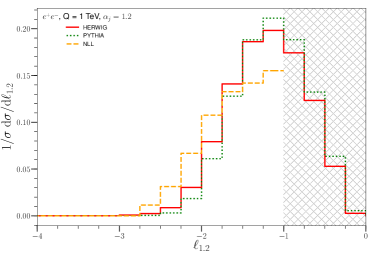
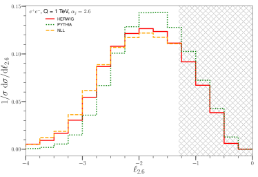
We begin by showing a comparison between the Herwig, Pythia and analytic predictions for the single angularity distribution in fig. 4. We find good agreement between the Herwig and Pythia results. The analytical result agrees very well with the numerical results for the angularity , but shows some deviations for . The reason for this is that the resummation region gets squeezed between the fixed-order region and the non-perturbative region666While we do not include hadronization, this region is sensitive to the unphysical shower cut off..
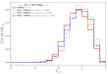
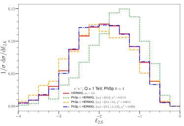
In fig. 5, we show results for two examples, obtained through reweighing with the best possible set of angularities. In the left panel we show the results for , where the performance for each is comparable. In the right panel, where we show , there is a dramatic improvement going from the best possible reweighing with angularity to the best result for reweighed angularities. We stress that the best set of angularities is obtained through a global minimization and is thus not optimized for any specific . The improvement from to is substantial, although not as dramatic.
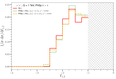
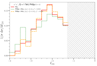
Fig. 6 shows the corresponding set of plots constructed by reweighing the NLL resummed results obtained from the calculation in sec. 3. In this case we have restricted the set of angularities that we examine to with instead, and we have used the “best set” of one or two angularities obtained from the analogous procedure done with Herwig. The restriction on the angularity exponents that we consider is chosen such that it allows for a sufficient number of bins in the analytical resummation to be populated, which is otherwise not the case for lower values of . To focus solely on the differences that arise due to reweighing with a different number of angularities, all the distributions that enter in these plots are obtained from projecting the full three-dimensional distribution with angularity exponents . The reason for this is that the projection of an analytically resummed cross section involving a higher number of angularities down to a cross section involving a lower number of angularities does not exactly agree with the corresponding cross section obtained from a direct analytic calculation, i.e. without any projection. A more in-depth discussion is relegated to app. A. With these comments in mind, we note that the reweighed results of fig. 6 show a similar trend as those of fig. 5, constructed using Herwig distributions.
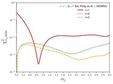
To indicate the improvement obtained over the full domain of considered angularities, we show the goodness-of-fit, for the best set of reweighed angularities as a function of in the left panel of fig. 7. For , one would expect that goes to zero for the best single angularity. However, we take the median of 11 replicas and the optimal single angularity is not the same for each of these. On the other hand, is always part of the set of best angularities for . It is clear that the case performs substantially better than , though there are a few angularities for which performs worse. This happens because they are close to the best single angularity and therefore reproduced very well by , but not as well for since the best two angularities are further away. For , there is a non-negligible, but less significant, improvement over .
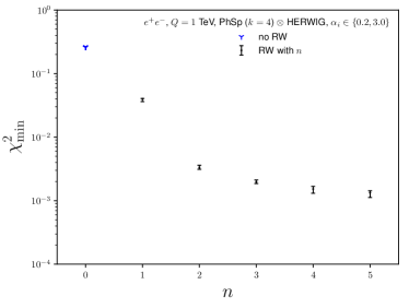
Finally, in the right panel of fig. 7, we show the minimum goodness-of-fit for . For this is the global minimum, whereas for the results were obtained iteratively, as described in sec. 2. For comparison we include , which simply states how well pure phase-space predictions (without any reweighing) describe the angularity distributions in Herwig, thus providing a baseline. The black error bars correspond to roughly one standard deviation, having been constructed from the spread of the 7 most central replicas out of a produced total of 11 replicas. The dots represent the median of the replicas. One can again observe a substantial improvement from to and a smaller but still visible improvement from to . The degree of improvement for going to or reweighed angularities is much smaller.
In app. A.1 we provide plots that demonstrate the robustness of our results under different variations. These include the use of Pythia as the Monte Carlo for the reweighing, considering either 5- or 6-body phase space, restricting the values of angularity exponents, and considering lower or higher center-of-mass energies. We also show results that discuss the quality of the projections from higher-dimensional distributions and the impact of these on the reweighing procedure in app. A.2.
5 Conclusions
We have investigated the benefits and limitations of joint resummation of large logarithms, using as an example the resummation of angularities in collisions. A major part of this work involved the development of an analytical method to jointly resum, at next-to-leading logarithmic order, any number of angularities. This was achieved using factorization theorems derived in the SCET formalism. While the joint resummation of two angularities had been studied before Larkoski:2014tva ; Procura:2014cba ; Procura:2018zpn , identifying all the regimes and relevant modes, and estimating the power corrections to connect them becomes more complicated for three (or more) angularities. This can be extended to processes with jets in hadronic collisions, in which case gluon jets also enter, and non-global logarithms Dasgupta:2001sh arise from soft radiation that simultaneously contributes to the angularities (measured on the jet) and the out-of-jet region.
Taking distributions obtained from this analytical resummation, as well as from the Herwig and Pythia Monte Carlo parton showers, we have studied whether employing them to reweigh a flat phase-space generator leads to improved predictions for other angularities (not used as input) via kinematic correlations. We have found an order of magnitude improvement when reweighing by distributions of two angularities over using only one, demonstrating the benefit of joint resummation. Reweighing with three or more angularities provides further improvement, albeit with a diminishing effect. The robustness of our conclusions is demonstrated by varying parts of our setup.
Our study shows that reweighing leads to improved predictions, particularly if the observable used in the reweighing procedure is similar to the observable of interest. Augmenting Monte Carlo parton showers by analytic resummation at NLL is probably not that useful, due to the sizable perturbative uncertainty at this order. However, this could be improved by matching the NLL to a fixed-order calculation. Furthermore, the factorization formulae presented here are not limited to a specific resummation order, and in principle all ingredients needed to NNLL are the same as for two angularities in ref. Procura:2018zpn . The reason for this is that, apart from the anomalous dimensions, all ingredients in the factorization formulae are only needed at one-loop order. They can therefore depend on at most two independent variables, so any additional angularities can be expressed in those two.
We believe that this approach opens up a new route towards precise and detailed (i.e. differential) predictions for collisions at the LHC, supplementing current advances in Monte Carlo parton showers. Such predictions are particularly important in an era in which the Standard Model is subjected to ever more stringent tests, and Machine Learning techniques are developed in order to uncover faint signals through detailed features in the data.
Acknowledgements.
This work was supported by the ERC grant ERC-STG-2015-677323, and the D-ITP consortium, a program of the Netherlands Organization for Scientific Research (NWO) that is funded by the Dutch Ministry of Education, Culture and Science (OCW). This article is based upon work from COST Action CA16201 PARTICLEFACE, supported by COST (European Cooperation in Science and Technology).Appendix A Additional plots
In this appendix we provide some additional plots that strengthen the universality of our conclusions, and briefly discuss the projections of the analytical resummed results.
A.1 Robustness of conclusions
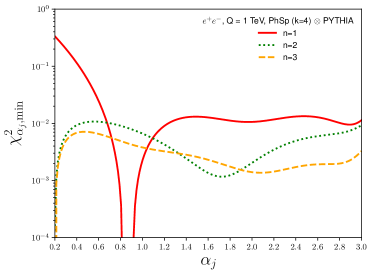
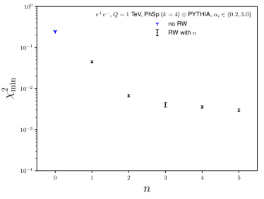
First of all, we show the analogue of fig. 7 using Pythia instead of Herwig. Specifically, the left panel of fig. 8 shows the goodness-of-fit, , as a function of . In this case, there is a single best angularity at for each of the replicas. Also, there is now a small region that does not improve from to . The right panel shows the global minimum goodness-of-fit for . The qualitative behavior is very similar to that in the right panel of fig. 7 for Herwig, but the values of are somewhat larger.
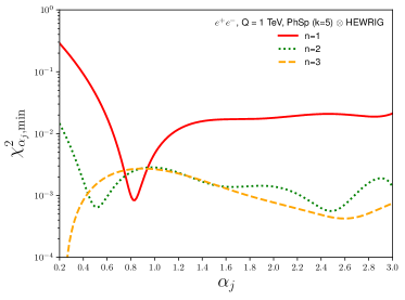
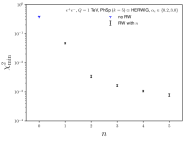
Fig. 9 is the analogue of fig. 7, but using -body flat phase space (i.e. ) instead of -body phase space. While the qualitative behavior is largely the same, there are some numerical differences that are mostly driven by statistical fluctuations, most visible in the left panel. Specifically, the sampling of the collinear and soft regions of phase space relevant for angularities is worse for .
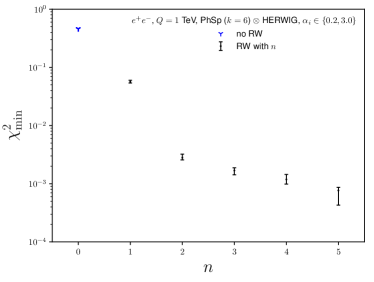
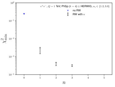
The left panel of fig. 10 is the analogue of the right panel of fig. 7, showing the minimum goodness-of-fit for -body phase space. As with , the larger number of phase-space particles worsens the sampling of the angularity phase space and hence increases the statistical fluctuations, reflected by the larger uncertainties. The right panel shows where we repeated the analysis for , restricting to the angularity exponents in the interval (again in steps of ). Because the total number of angularities is smaller, we only show the result of reweighing with angularities. This is also the reason for the faster convergence as function of the number of angularities used in the reweighing.
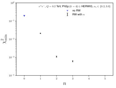
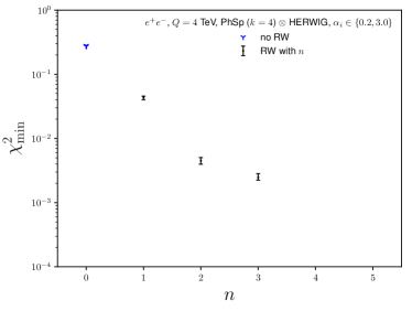
Finally, fig. 11 is the analogue of the right panel of fig. 7, but for different center-of-mass energies, GeV (left panel) and TeV (right panel). We do not show the reweighing with angularities. The qualitative behavior is similar as for TeV, but suggests that the reweighing procedure performs better for lower energies. This is in line with what one would expect from the increase in jet entropy with Neill:2018uqw .
A.2 Projections
In fig. 6 we showed results obtained by applying the reweighing procedure to analytical resummed results, all derived from the same multi-dimensional calculation. Here we comment briefly on the issues leading to this approach, and show results for an alternative method.
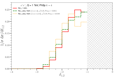
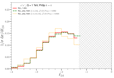
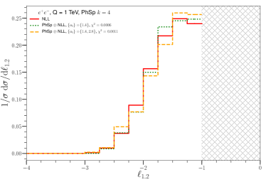
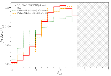
Fig. 12 shows the projections from higher-dimensional analytical results down to two specific angularity choices and . The yellow dotted and green dashed curves represent the projection from the indicated three-dimensional and two-dimensional cross section respectively. The red curve shows the directly determined cross section differential in the single angularity. The figure clearly illustrates that the curves are not identical and that projections differ more in comparison to the one-dimensional distribution if one starts from higher-dimensional cross sections. This fact is quantified in the between the one-dimensional resummed angularity distribution and each of the projections. Note that there is no corresponding issue for the Herwig and Pythia results, since they originate from fully exclusive events.
We suspect that this discrepancy is largely due to binning issues. As described in sec. 3.1, the number of distinct kinematic regions in phase space increases dramatically when cross sections differential in more angularities are considered. The result of the differential cross section in (the center of) each bin is obtained by determining the cumulative cross section on the edges of the bin777The use of cumulative cross sections is required to, at least theoretically, enable the recovery of the inclusive cross section Abbate:2010xh ; Almeida:2014uva ; Alioli:2015toa ; Bertolini:2017eui . and taking a numerical derivative. Due to the relatively small number of bins and the increasing number of kinematic regions, situations in which the edges and the center of a bin lie in different kinematic regions might occur. In these cases, the prediction of the spectrum (at the center of the bin) is obtained from input provided by cumulative distributions obtained from factorization formulas that are not valid at that point. As this is a binning issue, we expect the effect to diminish when a larger number of bins is considered.
Appendix B Resummation
The perturbative functions occurring in the factorization formula in eq. (16) are renormalized through
| (45) |
with anomalous dimensions given by
| (46) |
The cusp anomalous dimension to two loops is given by Korchemsky:1987wg
| (47) |
The one-loop non-cusp anomalous dimensions are given by
| (48) |
To NLL accuracy, the evolution kernels occurring in the resummed cumulative cross section in eq. (3.3) are given by
| (49) |
where has been defined. The required one- and two-loop coefficients of the beta function in the scheme are given by Tarasov:1980au
| (50) |
References
- (1) C. F. Berger, T. Kucs and G. F. Sterman, Event shape / energy flow correlations, Phys. Rev. D68 (2003) 014012 [hep-ph/0303051].
- (2) M. Bahr et al., Herwig++ Physics and Manual, Eur. Phys. J. C58 (2008) 639 [0803.0883].
- (3) J. Bellm et al., Herwig 7.0/Herwig++ 3.0 release note, Eur. Phys. J. C76 (2016) 196 [1512.01178].
- (4) J. Bellm et al., Herwig 7.1 Release Note, 1705.06919.
- (5) T. Sjöstrand, S. Ask, J. R. Christiansen, R. Corke, N. Desai, P. Ilten et al., An Introduction to PYTHIA 8.2, Comput. Phys. Commun. 191 (2015) 159 [1410.3012].
- (6) S. Höche, D. Reichelt and F. Siegert, Momentum conservation and unitarity in parton showers and NLL resummation, JHEP 01 (2018) 118 [1711.03497].
- (7) M. Dasgupta, F. A. Dreyer, K. Hamilton, P. F. Monni and G. P. Salam, Logarithmic accuracy of parton showers: a fixed-order study, JHEP 09 (2018) 033 [1805.09327].
- (8) G. Bewick, S. Ferrario Ravasio, P. Richardson and M. H. Seymour, Logarithmic Accuracy of Angular-Ordered Parton Showers, 1904.11866.
- (9) S. Jadach, A. Kusina, W. Placzek and M. Skrzypek, On the dependence of QCD splitting functions on the choice of the evolution variable, JHEP 08 (2016) 092 [1606.01238].
- (10) H. T. Li and P. Skands, A framework for second-order parton showers, Phys. Lett. B771 (2017) 59 [1611.00013].
- (11) S. Höche and S. Prestel, Triple collinear emissions in parton showers, Phys. Rev. D96 (2017) 074017 [1705.00742].
- (12) S. Höche, F. Krauss and S. Prestel, Implementing NLO DGLAP evolution in Parton Showers, JHEP 10 (2017) 093 [1705.00982].
- (13) Z. Nagy and D. E. Soper, Effects of subleading color in a parton shower, JHEP 07 (2015) 119 [1501.00778].
- (14) J. Isaacson and S. Prestel, Stochastically sampling color configurations, Phys. Rev. D99 (2019) 014021 [1806.10102].
- (15) S. Plätzer, M. Sjodahl and J. Thorén, Color matrix element corrections for parton showers, JHEP 11 (2018) 009 [1808.00332].
- (16) P. Richardson and S. Webster, Spin Correlations in Parton Shower Simulations, 1807.01955.
- (17) J. R. Andersen, H. M. Brooks and L. Lönnblad, Merging High Energy with Soft and Collinear Logarithms using HEJ and PYTHIA, JHEP 09 (2018) 074 [1712.00178].
- (18) A. Banfi, B. K. El-Menoufi and P. F. Monni, The Sudakov radiator for jet observables and the soft physical coupling, JHEP 01 (2019) 083 [1807.11487].
- (19) G. Bell, A. Hornig, C. Lee and J. Talbert, angularity distributions at NNLL′ accuracy, JHEP 01 (2019) 147 [1808.07867].
- (20) J. C. Collins, D. E. Soper and G. F. Sterman, Factorization for Short Distance Hadron - Hadron Scattering, Nucl. Phys. B261 (1985) 104.
- (21) J. C. Collins, D. E. Soper and G. F. Sterman, Soft Gluons and Factorization, Nucl. Phys. B308 (1988) 833.
- (22) J. C. Collins, D. E. Soper and G. F. Sterman, Factorization of Hard Processes in QCD, Adv. Ser. Direct. High Energy Phys. 5 (1989) 1 [hep-ph/0409313].
- (23) A. Banfi, G. P. Salam and G. Zanderighi, Semi-numerical resummation of event shapes, JHEP 01 (2002) 018 [hep-ph/0112156].
- (24) A. Banfi, G. P. Salam and G. Zanderighi, Principles of general final-state resummation and automated implementation, JHEP 03 (2005) 073 [hep-ph/0407286].
- (25) A. Banfi, H. McAslan, P. F. Monni and G. Zanderighi, A general method for the resummation of event-shape distributions in annihilation, JHEP 05 (2015) 102 [1412.2126].
- (26) C. W. Bauer, S. Fleming and M. E. Luke, Summing Sudakov logarithms in in effective field theory, Phys. Rev. D63 (2000) 014006 [hep-ph/0005275].
- (27) C. W. Bauer, S. Fleming, D. Pirjol and I. W. Stewart, An Effective field theory for collinear and soft gluons: Heavy to light decays, Phys. Rev. D63 (2001) 114020 [hep-ph/0011336].
- (28) C. W. Bauer and I. W. Stewart, Invariant operators in collinear effective theory, Phys. Lett. B516 (2001) 134 [hep-ph/0107001].
- (29) C. W. Bauer, D. Pirjol and I. W. Stewart, Soft collinear factorization in effective field theory, Phys. Rev. D65 (2002) 054022 [hep-ph/0109045].
- (30) H.-n. Li, Unification of the and threshold resummations, Phys. Lett. B454 (1999) 328 [hep-ph/9812363].
- (31) E. Laenen, G. F. Sterman and W. Vogelsang, Recoil and threshold corrections in short distance cross-sections, Phys. Rev. D63 (2001) 114018 [hep-ph/0010080].
- (32) A. Kulesza, G. F. Sterman and W. Vogelsang, Joint resummation in electroweak boson production, Phys. Rev. D66 (2002) 014011 [hep-ph/0202251].
- (33) A. Kulesza, G. F. Sterman and W. Vogelsang, Joint resummation for Higgs production, Phys. Rev. D69 (2004) 014012 [hep-ph/0309264].
- (34) G. Lustermans, W. J. Waalewijn and L. Zeune, Joint transverse momentum and threshold resummation beyond NLL, Phys. Lett. B762 (2016) 447 [1605.02740].
- (35) S. Marzani and V. Theeuwes, Vector boson production in joint resummation, JHEP 02 (2017) 127 [1612.01432].
- (36) C. Muselli, S. Forte and G. Ridolfi, Combined threshold and transverse momentum resummation for inclusive observables, JHEP 03 (2017) 106 [1701.01464].
- (37) R. D. Ball, M. Bonvini, S. Forte, S. Marzani and G. Ridolfi, Higgs production in gluon fusion beyond NNLO, Nucl. Phys. B874 (2013) 746 [1303.3590].
- (38) M. Bonvini and S. Marzani, Double resummation for Higgs production, Phys. Rev. Lett. 120 (2018) 202003 [1802.07758].
- (39) S. Marzani, Combining and small- resummations, Phys. Rev. D93 (2016) 054047 [1511.06039].
- (40) M. Procura, W. J. Waalewijn and L. Zeune, Resummation of Double-Differential Cross Sections and Fully-Unintegrated Parton Distribution Functions, JHEP 02 (2015) 117 [1410.6483].
- (41) G. Lustermans, J. K. L. Michel, F. J. Tackmann and W. J. Waalewijn, Joint two-dimensional resummation in and -jettiness at NNLL, JHEP 03 (2019) 124 [1901.03331].
- (42) C. W. Bauer, F. J. Tackmann, J. R. Walsh and S. Zuberi, Factorization and Resummation for Dijet Invariant Mass Spectra, Phys. Rev. D85 (2012) 074006 [1106.6047].
- (43) P. Pietrulewicz, F. J. Tackmann and W. J. Waalewijn, Factorization and Resummation for Generic Hierarchies between Jets, JHEP 08 (2016) 002 [1601.05088].
- (44) A. J. Larkoski, I. Moult and D. Neill, Toward Multi-Differential Cross Sections: Measuring Two Angularities on a Single Jet, JHEP 09 (2014) 046 [1401.4458].
- (45) M. Procura, W. J. Waalewijn and L. Zeune, Joint resummation of two angularities at next-to-next-to-leading logarithmic order, JHEP 10 (2018) 098 [1806.10622].
- (46) A. Banfi, F. Caola, F. A. Dreyer, P. F. Monni, G. P. Salam, G. Zanderighi et al., Jet-vetoed Higgs cross section in gluon fusion at N3LO+NNLL with small- resummation, JHEP 04 (2016) 049 [1511.02886].
- (47) D. W. Kolodrubetz, P. Pietrulewicz, I. W. Stewart, F. J. Tackmann and W. J. Waalewijn, Factorization for Jet Radius Logarithms in Jet Mass Spectra at the LHC, JHEP 12 (2016) 054 [1605.08038].
- (48) A. Hornig, D. Kang, Y. Makris and T. Mehen, Transverse Vetoes with Rapidity Cutoff in SCET, JHEP 12 (2017) 043 [1708.08467].
- (49) J. K. L. Michel, P. Pietrulewicz and F. J. Tackmann, Jet Veto Resummation with Jet Rapidity Cuts, JHEP 04 (2019) 142 [1810.12911].
- (50) X. Liu, S.-O. Moch and F. Ringer, Threshold and jet radius joint resummation for single-inclusive jet production, Phys. Rev. Lett. 119 (2017) 212001 [1708.04641].
- (51) X. Liu, S.-O. Moch and F. Ringer, Phenomenology of single-inclusive jet production with jet radius and threshold resummation, Phys. Rev. D97 (2018) 056026 [1801.07284].
- (52) A. J. Larkoski, I. Moult and B. Nachman, Jet Substructure at the Large Hadron Collider: A Review of Recent Advances in Theory and Machine Learning, 1709.04464.
- (53) E. M. Metodiev, B. Nachman and J. Thaler, Classification without labels: Learning from mixed samples in high energy physics, JHEP 10 (2017) 174 [1708.02949].
- (54) T. Cohen, M. Freytsis and B. Ostdiek, (Machine) Learning to Do More with Less, JHEP 02 (2018) 034 [1706.09451].
- (55) E. M. Metodiev and J. Thaler, Jet Topics: Disentangling Quarks and Gluons at Colliders, Phys. Rev. Lett. 120 (2018) 241602 [1802.00008].
- (56) A. Andreassen, I. Feige, C. Frye and M. D. Schwartz, JUNIPR: a Framework for Unsupervised Machine Learning in Particle Physics, Eur. Phys. J. C79 (2019) 102 [1804.09720].
- (57) K. Datta and A. Larkoski, How Much Information is in a Jet?, JHEP 06 (2017) 073 [1704.08249].
- (58) R. Kleiss, W. J. Stirling and S. D. Ellis, A New Monte Carlo Treatment of Multiparticle Phase Space at High-energies, Comput. Phys. Commun. 40 (1986) 359.
- (59) S. Plätzer, RAMBO on diet, 1308.2922.
- (60) S. Catani, Y. L. Dokshitzer, M. Olsson, G. Turnock and B. R. Webber, New clustering algorithm for multi-jet cross-sections in annihilation, Phys. Lett. B269 (1991) 432.
- (61) G. Salam, Scheme, Unpublished .
- (62) D. Bertolini, T. Chan and J. Thaler, Jet Observables Without Jet Algorithms, JHEP 04 (2014) 013 [1310.7584].
- (63) A. J. Larkoski, D. Neill and J. Thaler, Jet Shapes with the Broadening Axis, JHEP 04 (2014) 017 [1401.2158].
- (64) B. Andersson, G. Gustafson, L. Lönnblad and U. Pettersson, Coherence Effects in Deep Inelastic Scattering, Z. Phys. C43 (1989) 625.
- (65) A. Hornig, C. Lee and G. Ovanesyan, Effective Predictions of Event Shapes: Factorized, Resummed, and Gapped Angularity Distributions, JHEP 05 (2009) 122 [0901.3780].
- (66) A. J. Larkoski, I. Moult and D. Neill, Non-Global Logarithms, Factorization, and the Soft Substructure of Jets, JHEP 09 (2015) 143 [1501.04596].
- (67) R. Abbate, M. Fickinger, A. H. Hoang, V. Mateu and I. W. Stewart, Thrust at N3LL with Power Corrections and a Precision Global Fit for , Phys. Rev. D83 (2011) 074021 [1006.3080].
- (68) L. G. Almeida, S. D. Ellis, C. Lee, G. Sterman, I. Sung and J. R. Walsh, Comparing and counting logs in direct and effective methods of QCD resummation, JHEP 04 (2014) 174 [1401.4460].
- (69) D. Bertolini, M. P. Solon and J. R. Walsh, Integrated and Differential Accuracy in Resummed Cross Sections, Phys. Rev. D95 (2017) 054024 [1701.07919].
- (70) M. G. Echevarría, T. Kasemets, J.-P. Lansberg, C. Pisano and A. Signori, Matching factorization theorems with an inverse-error weighting, Phys. Lett. B781 (2018) 161 [1801.01480].
- (71) J.-L. Lagrange, Mécanique Analytique. Veuve Desaint, rue du Foin S. Jacques, Paris, 1788.
- (72) M. Cacciari, G. P. Salam and G. Soyez, FastJet User Manual, Eur. Phys. J. C72 (2012) 1896 [1111.6097].
- (73) M. Dasgupta and G. P. Salam, Resummation of nonglobal QCD observables, Phys. Lett. B512 (2001) 323 [hep-ph/0104277].
- (74) D. Neill and W. J. Waalewijn, The Entropy of a Jet, 1811.01021.
- (75) S. Alioli, C. W. Bauer, C. Berggren, F. J. Tackmann and J. R. Walsh, Drell-Yan production at NNLLNNLO matched to parton showers, Phys. Rev. D92 (2015) 094020 [1508.01475].
- (76) G. P. Korchemsky and A. V. Radyushkin, Renormalization of the Wilson Loops Beyond the Leading Order, Nucl. Phys. B283 (1987) 342.
- (77) O. V. Tarasov, A. A. Vladimirov and A. Yu. Zharkov, The Gell-Mann-Low Function of QCD in the Three Loop Approximation, Phys. Lett. B93 (1980) 429.