Typical and extreme entropies of long-lived isolated quantum systems
Abstract
In this paper, we investigate and compare two well-developed definitions of entropy relevant for describing the dynamics of isolated quantum systems: bipartite entanglement entropy and observational entropy. In a model system of interacting particles in a one-dimensional lattice, we numerically solve for the full quantum behavior of the system. We characterize the fluctuations, and find the maximal, minimal, and typical entropy of each type that the system can eventually attain through its evolution. While both entropies are low for some “special” configurations and high for more “generic” ones, there are several fundamental differences in their behavior. Observational entropy behaves in accord with classical Boltzmann entropy (e.g. equilibrium is a condition of near-maximal entropy and uniformly distributed particles, and minimal entropy is a very compact configuration). Entanglement entropy is rather different: minimal entropy “empties out” one partition while maximal entropy apportions the particles between the partitions, and neither is typical. Beyond these qualitative results, we characterize both entropies and their fluctuations in some detail as they depend on temperature, particle number, and box size.
I Introduction
There are a number of distinct notions of entropy throughout physics – including for example definitions by Clausius, Boltzmann, Gibbs, von Neumann, Bekenstein-Hawking, and others. Often these notions qualitatively and quantitatively coincide in the limits of large numbers of particles in equilibrium under some set of constraints. Yet, physical systems are commonly in states that are far from equilibrium from the standpoint of fundamental physics. This raises the question of how these entropies differ out of equilibrium, to what degree their non-equilibrium behavior carries over from the equilibrium case, and how they correspond with our common notions of entropy such as a measure of disorder, an ability to perform work, or of the information content an observer has about the physical system.
In this work, we address these questions, by studying numerically the out-of-equilibrium behavior and the extreme fluctuations of two well-developed notions of entropy that are relevant and interesting in isolated thermodynamic quantum systems.
The first of the two entropies we consider is the entanglement entropy Page (1993); Grasselli (2014); Vidmar et al. (2017); Vidmar and Rigol (2017), which is a well-known entropy measure that quantifies the amount of non-local correlation between a subsystem and its compliment. It has a wide range of use and is important in understanding thermalization in isolated systems Deutsch et al. (2013); Zhang et al. (2015); Kaufman et al. (2016), quantum correlations and phase transitions Osborne and Nielsen (2002); Latorre et al. (2003); Vidal et al. (2003), the holographic principle and black hole entropy Emparan (2006); Nishioka (2018), as well as quantum information theory Mukohyama (1998); Unanyan and Fleischhauer (2005); Cho (2018). The second entropy we consider is the observational entropy Šafránek et al. (2019a, b, 2019), which is a generalization of Boltzmann entropy to quantum systems. Originally introduced by von Neumann von Neumann (2010, 1955) as a resolution to the fact that the [von Neumann] entropy does not increase in isolated systems, then briefly mentioned by Wehrl Wehrl (1978) as “coarse-grained entropy”, observational entropy has experienced a significant resurgence recently: it was generalized to multiple coarse-grainings Šafránek et al. (2019a, b), found to dynamically describe thermalization of isolated quantum Šafránek et al. (2019b); Lent (2019) and classical Šafránek et al. (2019) systems, discussed in relationship with other types of entropies Goldstein et al. (2019), found to increase under Markovian stochastic maps Gemmer and Steinigeweg (2014), and argued for as a natural candidate for entropy production Strasberg (2019) because its definition does not need an explicit temperature dependence.
Fluctuations in entropy were discussed far before these two types of entropy were introduced. The concept of entropy itself originated from Clausius, who laid the ground work for the second law of thermodynamics in the mid 19th century. It was Boltzmann who interpreted this concept statistically by inventing the well-known H-theorem Boltzmann (2003), which then led to a new definition of entropy that makes use of the statistical weight of the macrostate; for a given macrostate, the Boltzmann entropy is defined as , where is the number of constituent microstates. If the macrostate is an energy macrostate, this entropy is equal to thermodynamic entropy of the microcanonical ensemble Dunkel and Hilbert (2014); Hilbert et al. (2014); Schneider et al. (2014); Buonsante et al. (2016), and is proportional to Clausius’s entropy for systems in thermal equilibrium. Considering general (not necessarily energy) coarse-grainings, Boltzmann entropy is typically time-dependent and able to describe systems out of equilibrium, unlike the original definition of entropy Goldstein and Lebowitz (2004).111Note that when we make comparisons with the Boltzmann entropy, we actually mean the definition with general coarse-graining, not with energy coarse-graining which gives what is known as surface, or microcanonical entropy, which stays constant in an isolated system.
Boltzmann postulated that his entropy (the negative of the quantity ) always increases, and did not mention anything about possible downward fluctuations. This was criticizes by Zermelo, and Boltzmann explains in a later letter Brush (2004) that fluctuations in entropy are indeed unlikely but possible. For example, particles can in principle spontaneously contract into a small space (e.g., corner of a room), and correspond to a macrostate with lower (Boltzmann) entropy. This laid the groundwork for the study of fluctuations in entropy.
Much later, the relations that constrain the probability distribution of entropy fluctuations, i.e. the Fluctuation Theorems (FTs), became one of the most significant discoveries in non-equilibrium statistical physics Evans et al. (1993); Jarzynski (1997); Crooks (1999); Seifert (2012); Luposchainsky et al. (2013). Fluctuation relations for closed Talkner et al. (2008); Esposito et al. (2009); Rana et al. (2013) and open systems Esposito and Mukamel (2006); Brunelli et al. (2018); Manzano et al. (2018) pertain when an external force drives the system out of equilibrium.
These studies do not, however, explore how high or low the entropy of a quantum system can get if it has access to long time scales; this is the focus of this work. We do this for an isolated system, meaning that there is no exchange of energy or particles between the system and the surrounding, and the system evolves unitarily in the absence of any external drive. We also examine what the states with such extreme entropies looks like, how they compare for different types of entropies, and how they depend on system size and inverse temperature.
For generic (i.e. non-integrable) systems and at high temperature, entanglement entropy is equal to the thermodynamic entropy of a subsystem when the full system is in thermal equilibrium Popescu et al. (2006); Deutsch (2010); Deutsch et al. (2013); Santos et al. (2012); Kaufman et al. (2016) (with some corrections depending on the size of the system and strength of the interaction term). One might be tempted to infer that this entropy behaves similarly to Boltzmann entropy, even far from equilibrium. However the studies here of the extreme cases, show that entanglement entropy behaves very differently from that of Boltzmann entropy.
For example, there are macrostates with very many microstates that correspond to minimal entanglement entropy, and macrostates with very few microstates that correspond to maximal entanglement entropy. This shows that outside of equilibrium, entanglement entropy is fundamentally different from Boltzmann’s idea of entropy. A type of observational entropy, , on the other hand, associates larger entropy with larger macrostates, in accordance with Boltzmann.
The paper is structured as follows. In section II, we introduce the model at hand as well as the entropies under study. Next III, we examine the probability distribution of entropies over long time unitary evolution of the system and find the minimal and maximal values of entropy, given infinite time. We then compare the states with minimal, maximal and average entropy. In sections IV and V, we investigate the dependence of extreme values of entropy on system size and inverse temperature, respectively. We find that observational entropy never reaches values significantly below of its maximum value, as argued in a previous study Deutsch et al. (2020); this is in contrast to entanglement entropy of the small subsystem, which can reach values very close to zero in the limit of large system and bath size. In section VI, we provide numerical evidence that the result of Deutsch et al. (2020) is correct in the case of a physical system such as a fermionic lattice. Finally, in section VII, we connect the results of IV and VI: we show that for a highly localized state – i.e. a state for which the probability of localization in a small region is maximized – has minimal observational entropy, but not entanglement entropy. A short introduction to observational entropy can be found in the appendix A.
II Preliminaries
In this paper we consider a system of spin-less fermions in a 1-dimensional lattice of size with hard wall boundary conditions. The Hamiltonian describing fermions in sites is
| (1) |

(Due to hard-wall boundary conditions, terms with , , , and are not included.) Here and are fermionic annihilation and creation operators for site and is the local density operator. The nearest-neighbor (NN) and next-nearest-neighbor (NNN) hopping terms are respectively and and the interaction strengths are and as illustrated in Fig. 1.
In all simulations, we take , . In most simulations we take the inverse temperature to be (the reason for this choice is discussed in detail in section VI) with exceptions in Figures 6 and 7, where we illustrate the dependencies on temperature. We take number of particles to be either or , and we use different system sizes . The eigenvalues and eigenvectors of relevant Hamiltonians are computed using exact diagonalization. Using this method however limits us to small size systems due to the exponential rise in computation time and memory requirements with system size, hence the use of only or particle systems.
For entanglement entropy, we consider a bipartite system with Hilbert space , where A and B label the two partitions. Entanglement entropy is then defined as
| (2) |
where is the reduced density matrix. This entropy measures the amount of correlations, or “entanglement” between , the subsystem of interest, and , the bath. We take sizes of and to be and sites respectively. The exception to this is in Sec. VI where we consider the smaller subsystem to be of size sites in order for the subsystem to be large enough to contain all particles.
It worth mentioning that there are other definitions of entanglement entropy in which the system has multiple partitions and the entanglement entropy of the system is the sum of the entanglement entropies of each partition, i.e., the entanglement of each partition with the rest of the system Coffman et al. (2000); Rigolin et al. (2006); Deutsch et al. (2013). However, entanglement entropy is most commonly used in the context of bipartite systems in the literature, for example in relation to the Bekenstein-Hawking entropy of a black hole where the existence of a horizon leads to the bipartition of the degrees of freedom on a Cauchy surface Das et al. (2008). It is also common to use in studying quantum information protocols Bennett et al. (1993); Helwig et al. (2012) and understanding phases of matter Zhang et al. (2011); Jiang et al. (2012).
Next, we consider observational entropy with position and energy coarse-graining Šafránek et al. (2019a, b, 2019)
| (3) |
The positional (configuration) coarse-graining defines the partitions of the system (regions), and corresponds to measuring the number of particles in each of the regions. Energy coarse-graining is the coarse-graining given by energy eigenstates of the system, corresponding to measuring the total energy. In contrast with the entanglement entropy, there is not a subsystem or a bath; instead the entire system is divided into equally sized partitions. We set the size of each partition to be , so in a system of size , there will be number of partitions.
This entropy can be interpreted as “dynamical” thermodynamic entropy: it approximates the sum of thermodynamic entropies of each partition Šafránek et al. (2019b, 2019). As these partitions exchange particles and/or heat, this entropy rises to thermodynamic entropy of the entire system, which corresponds to partitions being in thermal equilibrium with each other. Therefore, can be loosely interpreted as a measure of how close to thermal equilibrium these partitions are. Precisely, it is an entropy that an observer would associate to a system where partitions are allowed to exchange energy but not particles, in the long-time limit. In our paper the particles do indeed exchange between the partitions, which is the reason why this quantity is time-dependent. For a short introduction into the framework of observational entropy, see Appendix A.
In all cases, we take the initial state to be a random pure thermal state (RPTS) (also known as thermal pure quantum or canonical thermal pure quantum state Sugiura and Shimizu (2012, 2013); Nakagawa et al. (2018)), which we define as
| (4) |
where ’s are the eigenstates of the total Hamiltonian, computed using exact diagonalization. The coefficients are random complex or real numbers, , and respectively, which leads to what will refer to as the complex or the real RPTS, with and obeying the standard normal distribution , and is the normalization constant. These states emulate a thermal state, while being pure. They are then evolved as .
We would like to point out that in the high-temperature limit, the observational entropy of such a state is at all times smaller than the canonical entropy , where and is the partition function. But in the long time limit and for this type of initial state, will grow to a value that is very similar to . (See Appendix A and Ref. Šafránek et al. (2019b) for more detail; this behavior will be illustrated in Figs. 5 and 7.)
III Distribution of fluctuations in entropy
In this section we explore downward and upward fluctuations in entanglement and observational entropy, and the states achieving extreme values in entropy.
First, we plot histogram of fluctuations in entanglement (Fig. 3) and observational entropy (Fig. 3), in a system of size : starting from a complex RPTS, the system is evolved, and at each small fixed time step we read out the value of entropy. Evolving for a long time, we therefore achieve sufficient statistics that tells us how likely it is to find any given value of entropy.
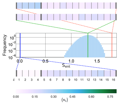
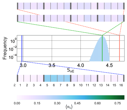
We can also ask what the minimum and maximum values of entropy are, given infinite time. Due to the exponential suppression of these extreme values, histogram cannot provide this minimum; we therefore use a minimization algorithm, explained below, and add the results to the histogram (orange and blue vertical lines in Figs. 3 and 3).
To find the extreme values of entropy we use the simplex search algorithm Nelder and Mead (1965). For a given and , we initialize the state in the same complex RPTS as the one we used to create the histograms in 3 and 3. We then find the maxima and minima for this initial state by maximizing over phases . As long as differences of ’s are irrational (or close to being irrational), this method must give the same result as maximizing over all times .
For each histogram, we provide three heat maps, displaying the particle density (, ) on the lattice sites for states of maximal, average, and minimal entropy.
III.1 Entanglement entropy
We can see that entanglement entropy achieves a minimal value that is very close to zero. We plot the heat map (below the histogram in Fig. 3) of the particle density of the state that corresponds to this minimum. We can see that in this situation, the particles moved almost entirely into the bath, thus naturally producing a separable state , where denotes vacuum in the subsystem. One might think that an alternative state , could also lead to zero entanglement entropy. However, as it is explained in the Section VI, one can not cluster all particles in a small region, when starting in a RPTS.
On the other hand, the state with maximum value of entanglement entropy is the one where the subsystem and the bath contain the same average number of particles. The smaller region therefore has a higher density of particles, as illustrated on the heat map. Intuitively, there have to be some particles in the subsystem and some in the bath, for any correlations to exist; and to create the maximum correlation, there should be the same amount of particles on either side. As can be seen from comparing the heat maps in Fig. 3, the state that has the maximum entanglement entropy is quite different from the thermal equilibrium state, where particles are distributed uniformly.
III.2 observational entropy
The minimum in is achieved by simply localizing the particles in one of the regions to the extent possible (it does not matter significantly which one, as they all give almost equal entropy; however, if one of the regions was smaller than the others, it would localize into this smallest region). The minimal value of never goes below about half of the maximal entropy; this, again, has to do with the inability to cluster all particles in a small region, when starting in an RPTS (see Sec. VII for a better intuition). The maximum of is given by a state where particles are uniformly distribution across all regions. is therefore in accordance with the Boltzmann entropy, in contrast to entanglement entropy.
IV Dependence of extreme values on the system size
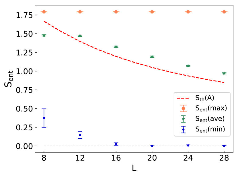
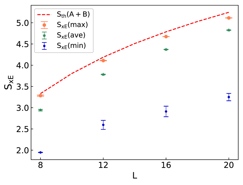
Next, we study the dependence of the minimum, maximum, and mean values of entropy on the system size. The minimum and maximum values are found using the minimization algorithm as in figures 3 and 3, and the average value is found by evolving the system for a long time.
IV.1 Entanglement entropy
These values are shown for entanglement entropy in Fig. 4. The size of the subsystem is kept fixed at while the system size (and hence the bath size) is varied such that . The number of particles and inverse temperature are kept fixed at and respectively. For each , we initialize the state in different complex RPTS, and then find the minima, maxima, and average values of entropy for each one of them. We plot the mean value of these six minima, maxima, and average, as well as the standard deviation (denoted as error bars), for a given system size .
We see the decrease in minimum entanglement entropy in Fig. 4 with increasing system size . As we discussed in the previous section in relation with Fig. 3, the entanglement between the subsystem and the bath is reduced mostly by moving all the particles into the bath. It is clear that as the bath (of size where is fixed) gets larger, it becomes easier to cluster all the particles in the larger bath, which makes the subsystem emptier, thus creating a state that resembles very closely a product state, and thus has a very small entanglement entropy.
It is important to emphasize that reduction in entanglement entropy is not achieved through disentangling the particles, but by disentangling the regions through the means of particles hopping and emptying the smaller region. Therefore the following question is raised: how much entropy would be reduced if particles’ hopping between the regions was forbidden? A simulation of this case – where the hopping terms between the two regions are zero – revealed that the reduction of entanglement entropy is much smaller: about a reduction.
The upper bound on maximum of entanglement entropy was derived in Faiez and Šafránek (2020) for closed, fermionic and bosonic systems. Specifically, in Fig. 4, where a (1-dimensional) fermionic lattice is considered, we have
| (5) |
In the case of and explored in Fig. 4, achieves exactly this upper bound at . The upper bound (5) is independent of the size of the bath in the limit of large , which explains the constant maximum value in Fig. 4 (the large in this case is already , and gives coincidentally the same value).
We should also note that, based on relation (5) found in Faiez and Šafránek (2020), one can see that this upper bound only depends on a few parameters, namely the size of the total system, size of the subsystem, the total number of particles (which is assumed to be fixed), and the assumption that the system is pure. Hence, it does not matter where the subsystem or bath is placed inside the system (for example in the middle or at the edge of the lattice).
The average entanglement entropy in the high temperature limit should be approximately equal to the thermodynamic entropy of the subsystem Popescu et al. (2006); Deutsch et al. (2013); Yamaguchi (2019), which is a fraction of the total thermodynamic entropy,
| (6) |
where is computed as the von Neumann entropy of a thermal state, i.e. for the full system, where and is the partition function, while where for the reduced system. Relation (6) has been confirmed in various numerical simulations Sørensen et al. (2007); Zhang et al. (2015); Kaufman et al. (2016). We see that this prediction, plotted as a red dashed line in Fig. 4, fits quite well with the data. (The relation (6) is only approximately true in the high temperature limit and not the low temperature limit, as is discussed in Hänggi et al. (2008); Hörhammer and Büttner (2008).)
Comparing the maximum value of entanglement entropy with the average, we note that is constant while decreases with . This is expected, since the average state spreads the particles uniformly over the entire system (creating less entanglement between the subsystem and the bath), while maximizing entanglement entropy maximizes correlations by distributing particles throughout the lattice such that the average number of particles in the subsystem follows the necessary but not sufficient condition for the state to be maximally entangled, stated in Ref. Faiez and Šafránek (2020). Based on this condition, the mean number of particles in sub-lattice is,
| (7) |
where , with is the probability of measuring particles in sub-lattice . We should note that in the numerical studies shown here, the average number of particles in the subsystem is equal to that of the bath but this is not in general the case. This discussion adds to Fig. 3 in demonstrating the difference between states leading to the average and the maximal entanglement entropy.
IV.2 Observational entropy
Using the same procedure, we find the mean values of minima, maxima, and averages of , and their variances, and plot them as a function of the system size in Fig. 5. Partitions have equal sizes fixed at and the system size (and therefore the number of partitions ) is varied.
The minimum values of observational entropy reduces to about a half of its maximum value independent of the system size, as long as it is large. These values could be indirectly estimated by simply assuming that the spatial localization is key in minimizing the entropy (see Fig. 9 and Eqs. (8) and (9)).
The maximum value of is almost exactly the same as the thermodynamic entropy of the full system, and very close to the average value of . This is expected from the theory Šafránek et al. (2019b), that shows , and differs from thermodynamic entropy by order-1 corrections (that depend on the energy distribution of the initial state), by corrections (that depend on how close the initial state is to the thermal state), both of which become irrelevant in the thermodynamic limit, and by finite-size corrections (coming from interaction energy between partitions), which become irrelevant when partitions are large enough.
V Dependence of extreme values on temperature
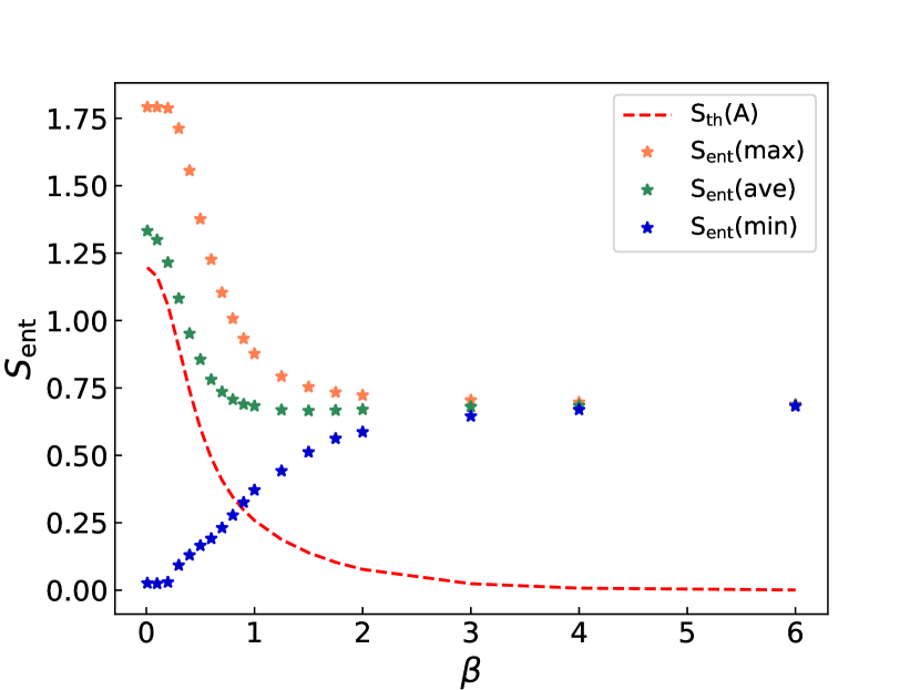
In this section, we look at the dependencies of the average and both extremes of and on inverse temperature . Each data point in Figures 6 and 7 are computed by taking the mean of the , , and average entropies over different complex RPTSs. We also included the thermodynamic entropy of the subsystem, , and of the total system, , in Figures 6 and 7 respectively.
V.1 Entanglement entropy
Fig. 6 plots the entanglement entropy versus . As one would expect, there are high fluctuations in the low (high temperature) limit. In this limit, the average entanglement entropy coincides with the thermodynamic entropy of the subsystem, which is known as the Volume law Nakagawa et al. (2018). Both maximal and minimal entanglement entropy diverge from the average at low , and are almost constant in this limit: (which is the high-temperature limit obtained previously in Fig. 4), and . There are almost no fluctuations in the opposite high (low temperature) limit, where the thermal state is almost identical to the ground state, and therefore it does not evolve. The entanglement entropy approaches a constant value given by the Area law Eisert et al. (2010); Laflorencie (2016); Cho (2018). The difference between entanglement entropy and thermodynamic entropy is discussed in more detail in Hörhammer and Büttner (2008).
V.2 Observational entropy
Fig. 7 plots the observational entropy versus , and we took the same settings as with entanglement entropy. One can notice two interesting features in this graph.
First, values of at high (low temperature) limit are quite large, and do not seem to follow the anymore. The fact that the is not zero in this low temperature limit is because measuring position does not commute with measuring energy. By measuring the position of the ground state, which is highly non-local, one would add a lot of energy to it, as well as uncertainty in energy. Therefore, since measures the total uncertainty when measuring the position first and then energy, this total uncertainty will be large. can be also interpreted as a thermodynamic entropy of the system, as if the numbers of particles in each bin were fixed, but the energy between the bins was still allowed to exchange Šafránek et al. (2019, 2019a, 2019b). It therefore makes sense that the value of this entropy is relatively large, since by measuring the position we fix the number of particles in each bin, and this state has a relatively large thermodynamic entropy. This effect gets to be smaller ( for high is smaller), when size of the partition becomes large compared to the size of the full system, since position measurement does not affect energy as much in that case. We note that this is a purely quantum effect, however, switching the order of coarse-grainings (while taking some small coarse-graining of width in energy as well), leads to an entropy that is bounded above by even at such low temperatures. (See Appendix A for details.) This is because measuring energy of a ground state does not affect this state at all, and additional measurement in position does not add any new information (see Theorem 8 in Šafránek et al. (2019b)). This effect was not noted in the original paper Šafránek et al. (2019b), mainly because defining microcanonical entropy at such low temperatures is problematic, as the energy density of states is not well defined.222Fig. 7 in Šafránek et al. (2019b) does not show nor microcanonical entropy for really low, or really high energies .
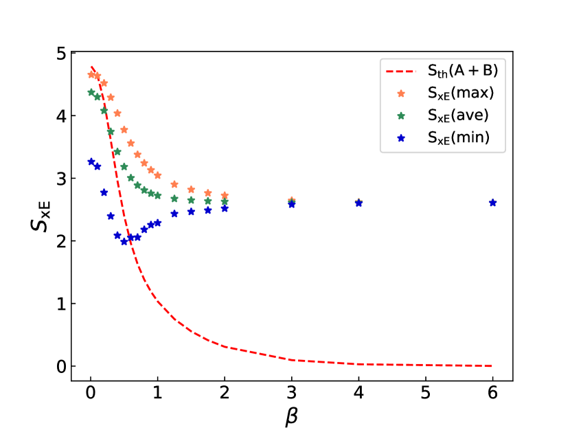
The second interesting feature of this graph is the dip in at . This dip is a result of two competing factors: first, by increasing the temperature, we increase the ability of the system to localize. Generally, localizing the system in one of the partitions leads to a decrease in (see Section VII). Thus, with high enough temperature the system is able to localize in one of the partitions of size and decrease the entropy. However, further increasing temperature does not help in decreasing anymore, as the further ability to localize is already below the resolution of the positional coarse-graining in , and its only effect is then an increase in the total thermodynamic entropy, and hence also an increase .
VI Maximal probability of localization
(a)
(b)
In this section we show numerically that the result of Deutsch et al. Deutsch et al. (2020) – shown analytically for a toy model with random energy eigenvectors as well as for a non-degenerate weakly interacting gas – holds true for a physical system of a fermionic lattice. We do this because in Sec. VII we would like to use this result to explain the connection, already hinted in the previous sections, between the spatial localization and the minimization of entropies.
In particular, Deutsch et al. showed that starting from a RPTS, under certain conditions, the maximum probability that all particles are localized into the subsystem of interest is in the case of initial real RPTS and in the case of complex RPTS. This, as shown in section VII, is key in minimizing .
We are going to require that the same conditions as in Deutsch et al. (2020) to be satisfied: The first condition is that the dimension of the subspace (the subspace of Hilbert space associated with “all particles being in the subsystem of interest”) is much smaller than the dimension of the full system, , which can be for example satisfied in the case of dilute gas (small number of particles) when the size of the subsystem of interest into which we localize the particles is much smaller than the size of the full system, . At the same time, the second condition is that the size of the subsystem is much larger than a thermal wavelength (specified below), . The third condition is that the size of the subsystem of interest, , is also much greater than the scattering length, i.e., we consider the Hamiltonian with only local interactions, leading to a weakly correlated system. However unlike what is used in Deutsch et al. (2020) – in which the energy eigenstates of the toy model are randomly distributed or are that of a non-degenerate weakly interacting gas – in our case the energy eigenstates are that of a Hamiltonian modeling a fermionic lattice.
First, we investigate the second condition, in more detail. At any value of , there exists a spatial scale known as the thermal wavelength such that (for example, in the case of an ideal gas, ). Qualitatively, is the minimum size of quantum wavepackets that describe the particles in a given system at a given temperature. Because of this relation between and , we can focus on the dependence of on .
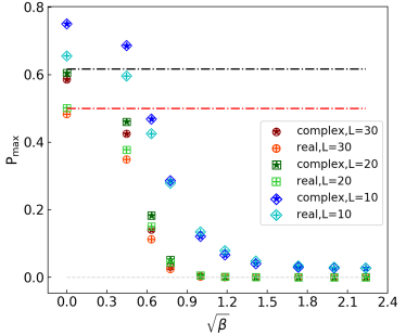
Therefore, in Fig. 8(a) we study the maximum probability of localization for different values of while fixing the size of the box . We localize in the region of size , and use the lattice sizes , , and , with particles inside. We do this for both real and complex initial RPTSs.
We see that for cold systems (high ), the probability of localization is very small, in fact, approaches zero. This is in accordance with the result of Deutsch et al. (2020) which asserts that, in the limit of large such that , where is the dimension of the lattice (in our case ). Intuitively, since is the minimum size of quantum wavepackets, it makes sense that one can not localize the wavefunction in a subspace smaller than this length scale.
For hot systems (low ), the probability of localization achieves high values. One notices that for small systems for e.g. , the gap between for the real and complex wave functions disappears. This is trivial, since in this case, the size of the subsystem of interest is becoming comparable to that of the full system, and therefore it is very easy to localize all particles in it. For larger system sizes for e.g. all three conditions stated above are satisfied, and approaches constant values of in the case of real RPTSs and in the case of complex RPTSs. The low regime is further explored in Fig. 8(b).
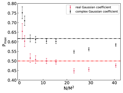
To generate this graph, we used the same algorithm to maximize probability as the one used in Deutsch et al. (2020), and . We start in different real and complex RPTSs, and for each one of them we perform the maximization procedure. We use three fermions and choose the small region to be sites. is plotted as a function of for both cases of complex and real RPTSs.
As one can see, when the system is hot enough, it is possible to localize all the particles into the small region, and the probability that we find them there is at most and for real and complex RPTSs respectively. The presence of some fluctuations is expected since our model is a real system with non-random energy eigenvectors. This numerically confirms that the results of Deutsch et al. Deutsch et al. (2020) also holds for a realistic quantum thermodynamic system such as ours, and we can apply this result in the next section.
VII Role of localization in extreme values of entropies
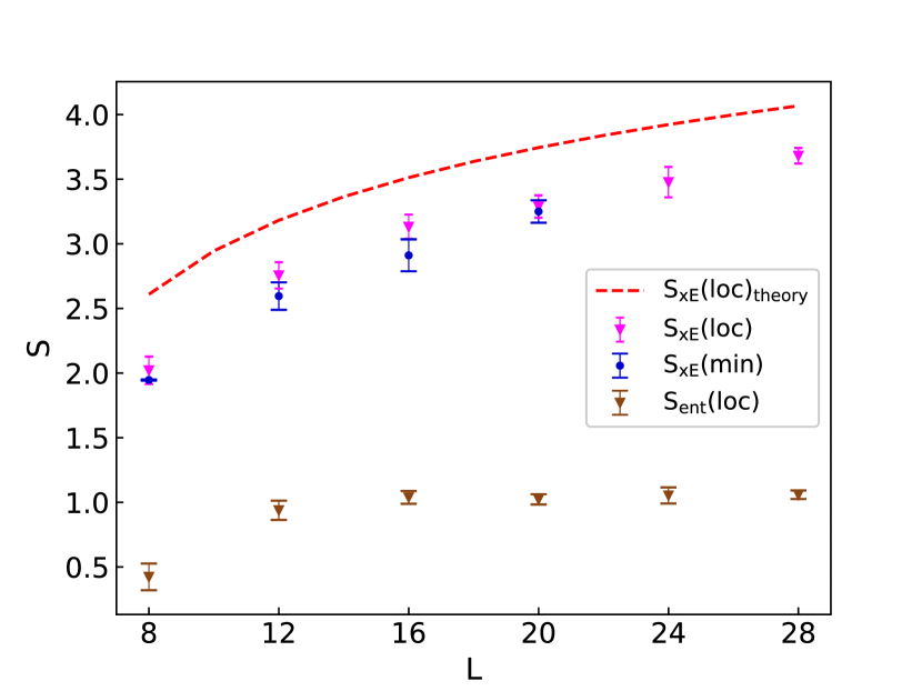
In figures 3 and 3 we showed that minimizing entanglement and observational entropy leads to a substantial probability of localization in the larger and smaller regions respectively. In this section, we investigate what happens to entanglement entropy when one localizes particles into the small region as opposed to the bath, and the extent to which the spatial localization plays a role in minimizing the .
We compute entropies of localized states, for and varying system sizes . We consider particles in the system, and temperature is fixed at , so that the three conditions from the previous section are satisfied. For each , we start in initial complex RPTSs, and localize them into a physical region of fixed size , by maximizing probability for each initial state. We then compute the mean values and standard deviations of and of such localized states, and plot them in Fig. 9. The mean values of (averaged over initial RPTSs) for system sizes of are .
is very close to the minimum (discussed in detail in Fig. 9), showing that spatial localization is key in minimizing . The theory predicts Deutsch et al. (2020)
| (8) |
for large (where ), which is bounded below by
| (9) |
which shows that cannot fall below a certain fraction of the total thermodynamic entropy of the system. Eq. (8) is plotted as a dashed line in Fig. 9 and as expected from Eq. (9), the ratio remains approximately constant for large .
The fact that and are almost the same and that is bounded by a fraction of thermodynamic entropy also explains why the minimum of in Fig. 3 does not go to zero, and why in Fig. 7 goes upwards for small (in the case of low ).
(a)
(b)
VIII Discussion and conclusion
In this paper, we have demonstrated the significantly different behavior of extreme values of entanglement and observational entropy by illustrating the behaviour of these entropies in and out of equilibrium and at different temperatures in an isolated quantum system. In particular we show that observational entropy behaves similarly to Boltzmann entropy, even in its extreme cases, i.e., far from equilibrium, while entanglement entropy does not. Indeed these entropies pertain to rather different physical features: observational entropy has the ability to quantify localization of particles and energy, while entanglement entropy measures non-local correlations, for systems both in and out of equilibrium.
With regards to extreme values, we found that starting from a random pure thermal state, can reach values very close to zero during the course of a unitary evolution, whereas there exists a non-zero lower bound for . We showed how these minimal values of the two entropies are achieved through localization in the larger and smaller region for and , respectively.
We found that in the high temperature limit, the maximum entanglement entropy between a smaller subsystem and the rest of the system, becomes very large in comparison with typical values, and this ratio grows with system size. This is because the typical value is the thermodynamic entropy for the smaller subsystem, which will tend to zero as total system size increases (at fixed particle number and subsystem size) but the maximum goes to a constant independent of total system size. On the other hand, the maximal observational entropy stays close to its typical value. The latter is qualitatively similar to classical Boltzmann entropy: the average – which is close to the most likely state – should be assigned a very high entropy.
The particle distribution given a state with maximum entanglement or observational entropy is also markedly different: in the former case, the particles distribute themselves throughout the lattice such that the average number of particles in the subsystem follows condition (7) in pursuit of maximizing correlations between the two subsystems, Whereas in the latter case, particles tend to distribute themselves uniformly, similar to what happens at thermal equilibrium.
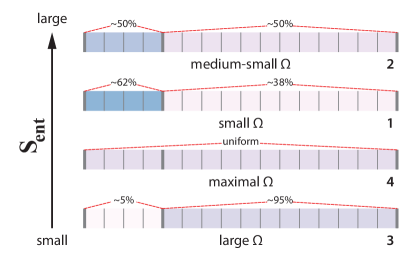
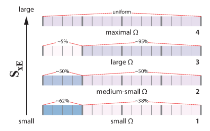
These findings are illustrated in Fig. 10. In particular, Fig. 10 (a) and (b) show entropies for various types of macrostates, described by their particle density, in order of smaller to higher entanglement and observational entropy, respectively. From the Boltzmann point of view, the size of the macrostate is determined by the number of microstates corresponding to the same macroscopic appearance: in this figure, size of the macrostate is the number of orthogonal quantum states that give the same distribution of particle density.
One notices that higher entanglement entropy does not necessarily mean that the macrostate is larger – the size of the macrostate appears to be rather unrelated to the amount of entanglement entropy. Specifically, it would be more likely to observe a state with minimal entanglement entropy as compared to the maximal entanglement entropy (as the former has a larger macrostate). The size of the macrostate and the entropy of the state match for the case of observational entropy, showing that (quantum) observational entropy matches well with the classical conception of Boltzmann entropy.
It should be noted that in this paper we focused on bipartite entanglement entropy, since it is very often used in literature. One could argue that multipartite entanglement entropy, defined as the sum of local von Neumann entropies, could behave similarly to and be more Boltzmann-like, meaning that the larger macrostates have associated higher values of entropy. 333This property would be however dependent upon having equally-sized regions, and the equivalence would break even when the size of a single region is different from others.
Because of its close relation to Boltzmann entropy, observational entropy could accompany the entanglement entropy to better understand the concept of thermalization in isolated quantum systems, and to illuminate the behavior of out-of-equilibrium states which lie at the heart of statistical mechanics. This entropy is also rather new in the field of quantum thermodynamics and hence further work on this particular entropy is of interest.
Experimentally, for example, observational entropy could be measured without the need to access the density matrix, and be useful in quantifying how thermalized a given state is. The extreme values of this entropy could possibly be probed as well, for extremely small systems such that the time it takes to reach these values is reasonably small and within reach in laboratories.
Finally, on a cosmological level, discussions of entropy and the arrow of time (e.g. Davies (1977); Aguirre and Gratton (2003); Albrecht and Sorbo (2004); Penrose (2004); Carroll and Chen (2004); Aguirre et al. (2012)) require a definition that applies to a truly closed system (like the Universe), out of equilibrium, and potentially for indefinitely long timescales over which large entropy fluctuations might occur. These discussions often employ an “informal” definition of entropy that in practice mixes different notions. Observational entropy applies in this context and is rigorously defined, and therefore may be very useful in these discussions. (The primarily remaining obstacle being a lack of understanding of the state-space of gravity and spacetime.) Could this definition of entropy, for example, tell us something new about the arrow of time in isolated quantum systems, and about how to understand extreme entropy fluctuations in the context of the arrow of time?
Extending this work to other types of observational entropies that are in accordance with thermodynamic entropy (such as “Factorized Observational Entropy” Šafránek et al. (2019b)) would be of interest as well. This could give us a broader understanding of this definition of entropy and non-equilibrium many-body quantum systems.
Acknowledgements.
This research was supported by the Foundational Questions Institute (FQXi.org) of which AA is Associate Director, and the Faggin Presidential Chair Fund.Appendix A Short introduction to observational entropy
Observational entropy is a generalization of Boltzmann entropy into quantum systems. It was mentioned but not developed by von Neumann in 1929 von Neumann (2010, 1955) then more recently rediscovered, developed, generalized to include multiple (even non-commuting) coarse-grainings, and connected to thermodynamics in Šafránek et al. (2019a, b), using the following construction:
Let us assume that the Hilbert space can be decomposed into a direct sum of orthogonal subspaces , where each subspace corresponds to a macrostate specifying a single macroscopic property of the system (such as energy or number of particles). Defining projector as the projector onto a subspace , the set forms a trace-preserving set of orthogonal projectors, denoted a coarse-graining. The probability that a quantum state is in a given macrostate can be calculated as . Equivalently, we can say that this is the probability that a system described by a quantum state will be found having a value of a macroscopic property defined by the coarse-graining, when performing a coarse-grained measurement on it in the basis given by the coarse-graining.
Assuming that an observer cannot distinguish between different microstates within the same macrostate with his/her macroscopic measurement, he/she associates the same probability to every microstate (given by a pure quantum state) in the macrostate. Given this inability to distinguish between different microstates within the same macrostate, we consider the Shannon entropy of the probabilities ,
| (10) |
This defines observational entropy with a single coarse-graining.
A generalization of this quantity for multiple coarse-grainings that allows many of its properties to be retained is
| (11) |
where multi-index denotes a set of macroscopic properties, is the probability of these properties being measured (in the given order), and denotes a joint Hilbert space volume of all systems that have properties measured in this order. Equivalently, we can call the volume of multi-macrostate .
An important property of is that it depends on the order of coarse-grainings, and that for any ordered set of coarse-grainings and any density matrix ,
| (12) | |||
| (13) |
In words, this means that observational entropy is lower bounded by the von Neumann entropy, which can be interpreted as an inherent uncertainty in a quantum system, upper bounded by the maximal uncertainty in the system, and that with each added coarse-graining, the observational entropy does not increase. These properties show that observational entropy can be interpreted as an observers’ uncertainty about the system, given that all that he/she can do is to perform a set of macroscopic measurements on this system.
Despite the intuitive interpretation of this general quantity, its physical meaning depends upon the coarse-graining. Several pertinent examples we have identified are as follows.
First is a coarse-graining in energy, , where is a projector onto a subspace associated with eigenvalue of the Hamiltonian (for non-degenerate Hamiltonians, is a projector onto a single energy eigenstate). Observational entropy then gives the equilibrium value of the thermodynamic entropy. For example, for a microcanonical state it gives the microcanonical entropy,
| (14) |
where denotes the energy density of states, while for the canonical state it gives the canonical entropy,
| (15) |
A second example, leading to time-dependence while still pertaining to thermodynamics, is the coarse-graining in local Hamiltonians, , where , , are projectors onto local energy eigenstates. The resulting entropy then measures how close to equilibrium these local regions are.
A third and closely-related example is , Eq. (3), which is the main focus of this paper. This observational entropy, coarse-grained first in local particle numbers, and then in total energy, can be interpreted as entropy that an observer would associate to a system where partitions are allowed to exchange energy but not particles, in the long-time limit. In our paper the particles do indeed exchange between the partitions, which is the reason why this quantity is time-dependent. is upper bounded by thermodynamic entropy (either canonical or microcanonical, depending on the spread in energies), and converges to it in the long-time limit in any non-integrable closed quantum system, up to small corrections (see Ref. Šafránek et al. (2019b)). is upper bounded by thermodynamic entropy and converges to it in the long-time limit only in the high-temperature limit (as can be seen in Fig. 7). A few other related entropies can be defined by considering a finite resolution in energy; these come with some subtleties, and resolve some slight issues in the behavior of the current definitions.444Note that switching the order of coarse-graining, leads to an entropy that is always lower than the thermodynamic entropy in both high and low-temperature limit as per Eq. (13), , but comes with its own set of problems (for example, it associates zero entropy to any energy eigenstate.) This can, however, be resolved by introducing a suitable resolution in measuring energy (not too low and not too high), which then leads to an entropy that associates microcanonical entropy to energy eigenstates, and an entropy that converges to in the long-time limit for states that are superpositions of many energy eigenstates. The fact that a suitable makes this entropy useful has been only discovered recently by us and only briefly touched upon in Šafránek et al. (2019), and is not discussed in the original papers Šafránek et al. (2019a, b), which in Appendix H of Šafránek et al. (2019b) claimed that is not a good definition of entropy (while it indeed is, as we have just explained). A similar problem happens with , which associates zero entropy to states consisting of local energy eigenstates, . Again, this can be resolved by introducing small but non-zero resolution in measuring local energies , which then defines an entropy that leads to the sum of local microcanonical entropies, .
We chose to study in this paper, because it is significantly easier to calculate, and since in most cases (especially in the high-temperature limit), all , , behave quite similarly.
References
- Page (1993) D. N. Page, Phys. Rev. Lett. 71, 1291 (1993).
- Grasselli (2014) F. Grasselli, Master’s thesis, Università degli Studi di Perugia (2014).
- Vidmar et al. (2017) L. Vidmar, L. Hackl, E. Bianchi, and M. Rigol, Phys. Rev. Lett. 119, 020601 (2017).
- Vidmar and Rigol (2017) L. Vidmar and M. Rigol, Phys. Rev. Lett. 119, 220603 (2017).
- Deutsch et al. (2013) J. M. Deutsch, H. Li, and A. Sharma, Phys. Rev. E 87, 042135 (2013).
- Zhang et al. (2015) L. Zhang, H. Kim, and D. A. Huse, Phys. Rev. E 91, 062128 (2015).
- Kaufman et al. (2016) A. M. Kaufman, M. E. Tai, A. Lukin, M. Rispoli, R. Schittko, P. M. Preiss, and M. Greiner, Science 353, 794 (2016).
- Osborne and Nielsen (2002) T. J. Osborne and M. A. Nielsen, Phys. Rev. A 66, 032110 (2002).
- Latorre et al. (2003) J. I. Latorre, E. Rico, and G. Vidal, Quant. Inf. Comput. 4, 48 (2003).
- Vidal et al. (2003) G. Vidal, J. I. Latorre, E. Rico, and A. Kitaev, Phys. Rev. Lett. 90, 227902 (2003).
- Emparan (2006) R. Emparan, J. High Energy Phys. 2006, 012 (2006).
- Nishioka (2018) T. Nishioka, Rev. Mod. Phys. 90, 035007 (2018).
- Mukohyama (1998) S. Mukohyama, Phys. Rev. D 58, 104023 (1998).
- Unanyan and Fleischhauer (2005) R. G. Unanyan and M. Fleischhauer, Phys. Rev. Lett. 95, 260604 (2005).
- Cho (2018) J. Cho, Phys. Rev. X 8, 031009 (2018).
- Šafránek et al. (2019a) D. Šafránek, J. M. Deutsch, and A. Aguirre, Phys. Rev. A 99, 010101(R) (2019a).
- Šafránek et al. (2019b) D. Šafránek, J. M. Deutsch, and A. Aguirre, Phys. Rev. A 99, 012103 (2019b).
- Šafránek et al. (2019) D. Šafránek, A. Aguirre, and J. M. Deutsch, arXiv:1905.03841 [cond-mat.stat-mech] (2019).
- von Neumann (2010) J. von Neumann, Eur. Phys. J. H 35, 201 (2010).
- von Neumann (1955) J. von Neumann, Mathematical foundations of quantum mechanics (Princeton university press, Princeton, 1955), pp. 410–416.
- Wehrl (1978) A. Wehrl, Rev. Mod. Phys 50, 221 (1978).
- Lent (2019) C. S. Lent, Phys. Rev. E 100, 012101 (2019).
- Goldstein et al. (2019) S. Goldstein, J. L. Lebowitz, Tumulka, and N. Zanghi, arXiv:1903.11870 [cond-mat.stat-mech] (2019).
- Gemmer and Steinigeweg (2014) J. Gemmer and R. Steinigeweg, Phys. Rev. E 89, 042113 (2014).
- Strasberg (2019) P. Strasberg, arXiv:1906.09933 [cond-mat.stat-mech] (2019).
- Boltzmann (2003) L. Boltzmann, in The kinetic theory of gases: an anthology of classic papers with historical commentary (World Scientific, Hackensack, 2003), pp. 262–349.
- Dunkel and Hilbert (2014) J. Dunkel and S. Hilbert, Nat. Phys. 10, 67 (2014).
- Hilbert et al. (2014) S. Hilbert, P. Hänggi, and J. Dunkel, Phys. Rev. E 90, 062116 (2014).
- Schneider et al. (2014) U. Schneider, S. Mandt, A. Rapp, S. Braun, H. Weimer, I. Bloch, and A. Rosch, arXiv:1407.4127 [cond-mat.quant-gas] (2014).
- Buonsante et al. (2016) P. Buonsante, R. Franzosi, and A. Smerzi, Ann. Physics 375, 414 (2016).
- Goldstein and Lebowitz (2004) S. Goldstein and J. L. Lebowitz, Physica D 193, 53 (2004).
- Brush (2004) S. G. Brush, History of the Kinetic Theory of Gases (Istituto della Enciclopedia Italiana, 2004), vol. 7, chap. 44.
- Evans et al. (1993) D. J. Evans, E. G. D. Cohen, and G. P. Morriss, Phys. Rev. Lett. 71, 2401 (1993).
- Jarzynski (1997) C. Jarzynski, Phys. Rev. Lett. 78, 2690 (1997).
- Crooks (1999) G. E. Crooks, Phys. Rev. E 60, 2721 (1999).
- Seifert (2012) U. Seifert, Rep. Prog. Phys. 75, 126001 (2012).
- Luposchainsky et al. (2013) D. Luposchainsky, A. C. Barato, and H. Hinrichsen, Phys. Rev. E 87, 042108 (2013).
- Talkner et al. (2008) P. Talkner, P. Hänggi, and M. Morillo, Phys. Rev. E 77, 051131 (2008).
- Esposito et al. (2009) M. Esposito, U. Harbola, and S. Mukamel, Rev. Mod. Phys. 81, 1665 (2009).
- Rana et al. (2013) S. Rana, S. Lahiri, and A. Jayannavar, Pramana J. Phys. 80, 207 (2013).
- Esposito and Mukamel (2006) M. Esposito and S. Mukamel, Phys. Rev. E 73, 046129 (2006).
- Brunelli et al. (2018) M. Brunelli, L. Fusco, R. Landig, W. Wieczorek, J. Hoelscher-Obermaier, G. Landi, F. L. Semião, A. Ferraro, N. Kiesel, T. Donner, et al., Phys. Rev. Lett. 121, 160604 (2018).
- Manzano et al. (2018) G. Manzano, J. M. Horowitz, and J. M. R. Parrondo, Phys. Rev. X 8, 031037 (2018).
- Popescu et al. (2006) S. Popescu, A. J. Short, and A. Winter, Nat. Phys. 2, 754 (2006).
- Deutsch (2010) J. M. Deutsch, New J. Phys. 12, 075021 (2010).
- Santos et al. (2012) L. F. Santos, A. Polkovnikov, and M. Rigol, Phys. Rev. E 86, 010102(R) (2012).
- Deutsch et al. (2020) J. M. Deutsch, D. Šafránek, and A. Aguirre, Phys. Rev. E 101, 032112 (2020).
- Coffman et al. (2000) V. Coffman, J. Kundu, and W. K. Wootters, Phys. Rev. A 61, 052306 (2000).
- Rigolin et al. (2006) G. Rigolin, T. R. de Oliveira, and M. C. de Oliveira, Phys. Rev. A 74, 022314 (2006).
- Das et al. (2008) S. Das, S. Shankaranarayanan, and S. Sur, arXiv preprint arXiv:0806.0402 [gr-qc] (2008).
- Bennett et al. (1993) C. H. Bennett, G. Brassard, C. Crépeau, R. Jozsa, A. Peres, and W. K. Wootters, Phys. Rev. Lett. 70, 1895 (1993).
- Helwig et al. (2012) W. Helwig, W. Cui, J. I. Latorre, A. Riera, and H.-K. Lo, Phys. Rev. A 86, 052335 (2012).
- Zhang et al. (2011) Y. Zhang, T. Grover, and A. Vishwanath, Phys. Rev. Lett. 107, 067202 (2011).
- Jiang et al. (2012) H.-C. Jiang, Z. Wang, and L. Balents, Nat. Phys. 8, 902 (2012).
- Sugiura and Shimizu (2012) S. Sugiura and A. Shimizu, Phys. Rev. Lett. 108, 240401 (2012).
- Sugiura and Shimizu (2013) S. Sugiura and A. Shimizu, Phys. Rev. Lett. 111, 010401 (2013).
- Nakagawa et al. (2018) Y. O. Nakagawa, M. Watanabe, H. Fujita, and S. Sugiura, Nat. Comm. 9, 1635 (2018).
- Nelder and Mead (1965) J. A. Nelder and R. Mead, Comput. J. 7, 308 (1965).
- Faiez and Šafránek (2020) D. Faiez and D. Šafránek, Phys. Rev. B 101, 060401 (2020).
- Yamaguchi (2019) K. Yamaguchi, J. Phys. Soc. Jpn. 88, 064002 (2019).
- Sørensen et al. (2007) E. S. Sørensen, M.-S. Chang, N. Laflorencie, and I. Affleck, J. Stat. Mech. 2007, P08003 (2007).
- Hänggi et al. (2008) P. Hänggi, G.-L. Ingold, and P. Talkner, New J. Phys. 10, 115008 (2008).
- Hörhammer and Büttner (2008) C. Hörhammer and H. Büttner, J. Stat. Phys. 133, 1161 (2008).
- Eisert et al. (2010) J. Eisert, M. Cramer, and M. B. Plenio, Rev. Mod. Phys. 82, 277 (2010).
- Laflorencie (2016) N. Laflorencie, Phys. Rep. 646, 1 (2016).
- Davies (1977) P. C. W. Davies, The Physics of Time Asymmetry (University of California Press, Oakland, 1977).
- Aguirre and Gratton (2003) A. Aguirre and S. Gratton, Phys. Rev. D 67, 083515 (2003).
- Albrecht and Sorbo (2004) A. Albrecht and L. Sorbo, Phys. Rev. D 70, 063528 (2004).
- Penrose (2004) R. Penrose, The Road to Reality. A Complete Guide to the Laws of the Universe, Joanthan Cape (Random House, London, 2004).
- Carroll and Chen (2004) S. M. Carroll and J. Chen, arXiv:hep-th/0410270 [hep-th] (2004).
- Aguirre et al. (2012) A. Aguirre, S. M. Carroll, and M. C. Johnson, J. Cosmol. Astropart. Phys. 2012, 024 (2012).