Resonant Machine Learning Based on Complex Growth Transform Dynamical Systems

Oindrila Chatterjee,  and Shantanu Chakrabartty Both the authors are with the Department of Electrical and Systems Engineering, Washington University in St. Louis, St. Louis, Missouri 63130, USA. All correspondences regarding this manuscript should be addressed to shantanu@wustl.edu.This work was supported in part by a research grant from the National Science Foundation (ECCS:1550096).
Abstract

Traditional energy-based learning models associate a single energy metric to each configuration of variables involved in the underlying optimization process. Such models associate the lowest energy state to the optimal configuration of variables under consideration, and are thus inherently dissipative. In this paper we propose an energy-efficient learning framework that exploits structural and functional similarities between a machine learning network and a general electrical network satisfying the Tellegen’s theorem. In contrast to the standard energy-based models, the proposed formulation associates two energy components, namely, active and reactive energy to the network. This ensures that the network’s active-power is dissipated only during the process of learning, whereas the reactive-power is maintained to be zero at all times. As a result, in steady-state, the learned parameters are stored and self-sustained by electrical resonance determined by the network’s nodal inductances and capacitances. Based on this approach, this paper introduces three novel concepts: (a) A learning framework where the network’s active-power dissipation is used as a regularization for a learning objective function that is subjected to zero total reactive-power constraint; (b) A dynamical system based on complex-domain, continuous-time growth transforms which optimizes the learning objective function and drives the network towards electrical resonance under steady-state operation; and (c) An annealing procedure that controls the trade-off between active-power dissipation and the speed of convergence. As a representative example, we show how the proposed framework can be used for designing resonant support vector machines (SVMs), where we show that the support-vectors correspond to an LC network with self-sustained oscillations. We also show that this resonant network dissipates less active-power compared to its non-resonant counterpart.

Index Terms:
Electrical Resonance, Tellegen’s theorem, Energy-efficient learning models, Energy-based learning models, Complex domain machine learning, Support Vector Machines, Resonant Networks, Coupled Oscillators.

I Introduction

From an energy point of view, the dynamics of a machine learning framework is analogous to an electrical network since both the networks evolve over a conservation manifold to attain a low-energy state. In literature, this analogy has served as the basis for energy-based learning models, where the learning objective function is mapped to an equivalent network energy. [1, 2]. The network variables then evolve according to some physical principles subject to network constraints to seek out an energy optimal state.
Refer to caption
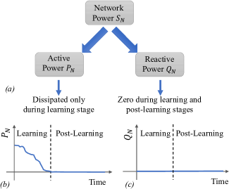
Figure 1: (a) The total or apparent power SNsubscript𝑆𝑁S_{N} of the electrical network comprising of the active-power PNsubscript𝑃𝑁P_{N} or the dissipated power and the reactive-power QNsubscript𝑄𝑁Q_{N} or the power used for energy-storage. The goal of the proposed resonant learning framework: (b) minimizing active-power PNsubscript𝑃𝑁P_{N} during learning and ensuring PN=0subscript𝑃𝑁0P_{N}=0, post-learning or steady-state; and (c) maintaining QN=0subscript𝑄𝑁0Q_{N}=0 in learning and post-learning phases.

However, even if the solution reached by such energy-based learning models may be optimal from the objective function point of view, it may not be the most energy-efficient solution when considering an actual physical implementation. This is because most of these formulations assume that the energy being minimized in the network is dissipative in nature. Whereas, in a physical electrical network, the total power SNsubscript𝑆𝑁S_{N} (also known as the apparent power) comprises not only of the dissipative component (also referred to as the active-power) but also a latent or stored non-dissipative component (also referred to as the reactive-power) [3, 4]. This is illustrated in Figure 1(a) and can be mathematically expressed as:

Total Network PowerSN=Active PowerPNTotal Network Powersubscript𝑆𝑁Active Powersubscript𝑃𝑁\displaystyle\text{Total Network Power}\enskip S_{N}=\text{Active Power}\enskip P_{N}
+j×Reactive PowerQN𝑗Reactive Powersubscript𝑄𝑁\displaystyle+j\times\enskip\text{Reactive Power}\enskip Q_{N} (1)

where j=1𝑗1j=\sqrt{-1} denotes the imaginary component. While the active-power PNsubscript𝑃𝑁P_{N} represents the rate-of-energy loss in the network, the reactive-power QNsubscript𝑄𝑁Q_{N} represents the rate of change in stored energy in the network’s electric and magnetic fields (typically modeled as lumped capacitive and inductive elements). In the design of electrical networks, reactive-power is generally considered to be a nuisance since it represents the latent power that does not perform any useful work [5, 6]. However, from the point of view of learning, the reactive-power could be useful not only for storing the learned parameters of the network, but could also improve the dynamics of the network during learning. In this paper, we propose such a framework which exploits both active and reactive network power for learning and memory. The objective will be to achieve a network power profile as illustrated in Figures 1 (b) and (c). During learning, the network will optimize its active-power (PNsubscript𝑃𝑁P_{N}) and under steady-state condition or post-learning, ensure PN=0subscript𝑃𝑁0P_{N}=0. The reactive-power (QNsubscript𝑄𝑁Q_{N}), on the other hand, will always be maintained at zero. This implies that the stored energy (mathematically - the time-integral of the reactive-power) is conserved across the learning and post-learning phases respectively. Thus, during the post-learning phase or in steady-state, the network will not dissipate any power, and the reactive energy is used to maintain its current network state or memory.

This steady-state condition corresponds to a state of electrical resonance, and in Section III we generalize this concept to a framework of resonant machine learning. To reach this steady-state, in Section IV, we present a dynamical system based on complex-domain continuous-time growth-transforms, which extends our previous work on growth transform networks using real-variables[7]. The complex-domain formulation allows manipulation of the relative phase between the voltage and current variables associated with the network nodes and thus is used to optimize the active-power dissipation during learning. While the approach could be applied to different learning networks, in Section V, we use this framework for designing resonant one-class support vector machines (SVMs) [8]. In this context, we also compare the performance of the resonant SVM model with its non-resonant variant on both synthetic and real datasets. Finally, Section VI concludes the paper with a brief discussion on the implication of the proposed model when applied to other network-based models that do not involve learning, for instance, the coupled oscillator networks[9].

The key contributions of the paper can be summarized as follows:

  • Contrary to standard energy-based models which optimize for a single energy metric, we map a learning problem to an electrical network with two energy components: dissipative(active) and non-dissipative(reactive) energy.

  • Active power dissipation is introduced as a regularizer in the original learning problem while enforcing zero total reactive power by driving the network into electrical resonance. This ensures zero active power dissipation in the post-learning stage.

  • We present a novel growth transform-based complex dynamical system for optimizing the cost function that ensures a resonant condition in steady-state.

  • We propose an annealing schedule that can trade-off speed of convergence with active-power dissipation for different applications.

I-A Notations

For the rest of the paper, we will follow the mathematical notations summarized in Table 1 below:

TABLE 1: Notations
Variable Definition
+subscript\mathbb{R}_{+} One-dimensional positive real vector space
Nsuperscript𝑁\mathbb{R}^{N} N-dimensional real vector space
\mathbb{C} One-dimensional complex vector space
|z|𝑧\lvert z\rvert magnitude of a complex variable z𝑧z
Re(z)𝑧\real(z) real part of a complex variable z𝑧z
Im(z)𝑧\imaginary(z) imaginary part of a complex variable z𝑧z
zsuperscript𝑧z^{*} complex conjugate of a complex variable z𝑧z
z(t)𝑧𝑡z(t) a continuous-time complex variable at time t𝑡t
znsubscript𝑧𝑛z_{n} a discrete-time complex variable at the nthsuperscript𝑛thn^{\text{th}} time step

II Background and Related works

II-A Energy-based Learning Models

The principle of minimum energy states that all self-organizing physical systems evolve dynamically over an intrinsic conservation manifold to attain their minimum energy configuration in the steady state[10]. Energy-based machine learning models follow a similar cue, where the goal is to find the optimal configuration of a predetermined energy landscape determined by the learning problem at hand[1, 11]. Some of the most notable examples of energy-based models are those based on the Ising model of statistical mechanics, like the Hopfield network[2], and its stochastic counterpart the Boltzmann machine [12] and its variants[13]. In these models, the network converges to the local minimum of a Lyapunov function in steady state. Another class of energy-based models (EBMs)[1] propose a unified learning framework by mapping the learning problem to a global scalar “energy function”. The algorithm minimizes a loss functional to seek out an optimal energy landscape that associates lowest energy to the observed configuration of variables involved in the underlying optimization process. These methods are essentially non-probabilistic, and often involve intractable integrals which require MCMC methods for normalization when applied to probabilistic frameworks. Different classes of optimization algorithms like contrastive divergence, contrastive hebbian learning, equilibrium propagation etc.[14] have been proposed for a variety of supervised, unsupervised and reinforcement learning applications[15, 16, 17, 18] in the context of energy-based models. However, all of these approaches consider an energy metric that solely depends on the learning task under consideration. This implies that in an analog implementation of the model, the optimal solution may not be the most energy-efficient one.

Refer to caption
Figure 2: Equivalent network model comprising of N𝑁N electrical nodes, with an inductance and capacitance element associated with each of the nodes. (a) Learning is equivalent to changing the values of inductive and capacitive elements; and (b) in steady-state the network is driven into electrical resonance.

II-B Complex-domain Machine Learning Models

A variety of complex domain learning models have been proposed in literature for different learning algorithms, e.g., complex neural networks, complex support vector machines, complex deep networks etc[19, 20, 21, 22, 23]. In addition to providing the phase variables which allow for another degree of freedom, other advantages of the complex domain operation have been shown in these works. It has been demonstrated that complex learning models lead to a richer set of dynamics, noise robustness and better convergence properties in the case of classification problems[20, 24, 25]. Moreover, phase information might provide additional insights in the context of many complex-valued physical signals (or complex domain transforms of physical signals, e.g., Fourier or wavelet transforms)[20, 26]. However, most of these complex learning models either treat the real and imaginary components of the signal separately, or do not utilize the entire phase space when operating in the complex domain.

III Optimization and Electrical Resonance
Refer to caption
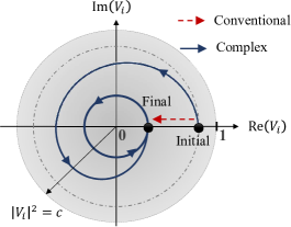
Figure 3: Illustration showing that operating in the complex domain allows different possible learning trajectories from an initial state to the final steady-state. Regularization with respect to the phase-factor could then be used to select the trajectory with an optimal active-power dissipation profile, and results in limit cycle oscillations in steady-state. The circles indicate the constant magnitude loci.

Consider an electrical network as shown in Figure 2(a), comprising of N𝑁N internal nodes. The voltage difference between the ithsuperscript𝑖thi^{\text{th}} and jthsuperscript𝑗thj^{\text{th}} nodes is denoted by Vijsubscript𝑉𝑖𝑗V_{ij}, with Vi0subscript𝑉𝑖0V_{i0} being the ithsuperscript𝑖thi^{\text{th}} nodal voltage with respect to ground terminal (referred to as the 0thsuperscript0th0^{\text{th}} node). Similarly, the current flowing between the ithsuperscript𝑖thi^{\text{th}} and jthsuperscript𝑗thj^{\text{th}} nodes is given by Iijsubscript𝐼𝑖𝑗I_{ij}, and Ii0subscript𝐼𝑖0I_{i0} denotes the current flowing out of the ithsuperscript𝑖thi^{\text{th}} node into the ground terminal. Then, according to the Tellegen’s theorem [27]:

iVijIij=0,subscript𝑖subscript𝑉𝑖𝑗superscriptsubscript𝐼𝑖𝑗0\sum\limits_{i}V_{ij}I_{ij}^{*}=0, (2)

which states that the total complex electrical power or apparent power is zero. Isolating the apparent power flowing from the nodes to the ground terminal from that flowing between the internal nodes, we have:

ij,0;j0(Vij)Iij+i(Vi0)Ii0=0subscriptformulae-sequence𝑖𝑗0𝑗0subscript𝑉𝑖𝑗superscriptsubscript𝐼𝑖𝑗subscript𝑖subscript𝑉𝑖0superscriptsubscript𝐼𝑖00\displaystyle\sum\limits_{i\neq j,0;j\neq 0}(V_{ij})I_{ij}^{*}+\sum\limits_{i}(V_{i0})I_{i0}^{*}=0
i=1NVi0Ii0=i,j=1NVijIijabsentsuperscriptsubscript𝑖1𝑁subscript𝑉𝑖0superscriptsubscript𝐼𝑖0superscriptsubscript𝑖𝑗1𝑁subscript𝑉𝑖𝑗superscriptsubscript𝐼𝑖𝑗\displaystyle\implies\sum\limits_{i=1}^{N}V_{i0}I_{i0}^{*}=-\sum_{i,j=1}^{N}V_{ij}I_{ij}^{*}
ST=SNabsentsubscript𝑆𝑇subscript𝑆𝑁\displaystyle\implies S_{T}=-S_{N}
PT+jQT=PNjQNabsentsubscript𝑃𝑇𝑗subscript𝑄𝑇subscript𝑃𝑁𝑗subscript𝑄𝑁\displaystyle\implies P_{T}+jQ_{T}=-P_{N}-jQ_{N}
|PT|=|PN|absentsubscript𝑃𝑇subscript𝑃𝑁\displaystyle\implies\lvert P_{T}\rvert=\lvert P_{N}\rvert
|QT|=|QN|absentsubscript𝑄𝑇subscript𝑄𝑁\displaystyle\implies\lvert Q_{T}\rvert=\lvert Q_{N}\rvert (3)

where ST=iVi0Ii0subscript𝑆𝑇subscript𝑖subscript𝑉𝑖0superscriptsubscript𝐼𝑖0S_{T}=\sum_{i}V_{i0}I_{i0}^{*} is the nodal apparent power, and PT=iRe{Vi0Ii0}subscript𝑃𝑇subscript𝑖subscript𝑉𝑖0superscriptsubscript𝐼𝑖0P_{T}=\sum_{i}\real\{V_{i0}I_{i0}^{*}\} and QT=iIm{Vi0Ii0}subscript𝑄𝑇subscript𝑖subscript𝑉𝑖0superscriptsubscript𝐼𝑖0Q_{T}=\sum_{i}\imaginary\{V_{i0}I_{i0}^{*}\} are the total active and reactive power consumed at the nodes. Similarly, SNsubscript𝑆𝑁S_{N}, PNsubscript𝑃𝑁P_{N} and QNsubscript𝑄𝑁Q_{N} represent the apparent, active and reactive power consumed due to current flow between the network nodes (other than the ground terminal). Note that this result holds even if active-power sources are embedded in the network, as shown in Figure 2(a). Thus, Equations (3) imply that if we minimize the active-power at the nodes of the network PTsubscript𝑃𝑇P_{T} subject to the constraint that the nodal reactive power QT=0subscript𝑄𝑇0Q_{T}=0, then the formulation would be equivalent to minimizing the network active-power PNsubscript𝑃𝑁P_{N} while ensuring that the network reactive power QN=0subscript𝑄𝑁0Q_{N}=0. This result can be expressed as:

min{Vi,Ii}𝒟=i=1N|Re{ViIi}|2subscript𝑉𝑖subscript𝐼𝑖min𝒟superscriptsubscript𝑖1𝑁superscriptsubscript𝑉𝑖superscriptsubscript𝐼𝑖2\displaystyle\underset{\{V_{i},I_{i}\in\mathbb{C}\}}{\text{min}}\quad\mathcal{D}=\sum\limits_{i=1}^{N}\lvert\real\{V_{i}I_{i}^{*}\}\rvert^{2}
s.t.iIm{ViIi}=0s.t.subscript𝑖subscript𝑉𝑖superscriptsubscript𝐼𝑖0\displaystyle\textit{s.t.}\quad\sum_{i}\imaginary\{V_{i}I_{i}^{*}\}=0 (4)

where we have used the notations Vi0=Visubscript𝑉𝑖0subscript𝑉𝑖V_{i0}=V_{i} and Ii0=Iisubscript𝐼𝑖0subscript𝐼𝑖I_{i0}=I_{i} for the sake of brevity. If we assume that the ithsuperscript𝑖thi^{\text{th}} node is associated with a lumped capacitance Cisubscript𝐶𝑖C_{i}, and a lumped inductance Lisubscript𝐿𝑖L_{i}, ensuring zero nodal reactive-power implies

i=1NVi(CidVidt)+(LidIidt)Ii=0,superscriptsubscript𝑖1𝑁subscript𝑉𝑖superscriptsubscript𝐶𝑖𝑑subscript𝑉𝑖𝑑𝑡subscript𝐿𝑖𝑑subscript𝐼𝑖𝑑𝑡superscriptsubscript𝐼𝑖0\sum\limits_{i=1}^{N}V_{i}\Big{(}C_{i}\dfrac{dV_{i}}{dt}\Big{)}^{*}+\Big{(}L_{i}\dfrac{dI_{i}}{dt}\Big{)}I_{i}^{*}=0, (5)

where (CidVidt)subscript𝐶𝑖𝑑subscript𝑉𝑖𝑑𝑡\Big{(}C_{i}\dfrac{dV_{i}}{dt}\Big{)} and (LidIidt)subscript𝐿𝑖𝑑subscript𝐼𝑖𝑑𝑡\Big{(}L_{i}\dfrac{dI_{i}}{dt}\Big{)} represent the current flowing through Cisubscript𝐶𝑖C_{i} and the voltage across Lisubscript𝐿𝑖L_{i} respectively. Equation (5) is equivalent to:

i=1N(12Ci|Vi|2+12Li|Ii|2)=E0,superscriptsubscript𝑖1𝑁12subscript𝐶𝑖superscriptsubscript𝑉𝑖212subscript𝐿𝑖superscriptsubscript𝐼𝑖2subscript𝐸0\displaystyle\sum_{i=1}^{N}\Big{(}\dfrac{1}{2}C_{i}\lvert V_{i}\rvert^{2}+\dfrac{1}{2}L_{i}\lvert I_{i}\rvert^{2}\Big{)}=E_{0}, (6)

where |Vi|2=ViVisuperscriptsubscript𝑉𝑖2subscript𝑉𝑖superscriptsubscript𝑉𝑖\lvert V_{i}\rvert^{2}=V_{i}V_{i}^{*} and |Ii|2=IiIisuperscriptsubscript𝐼𝑖2subscript𝐼𝑖superscriptsubscript𝐼𝑖\lvert I_{i}\rvert^{2}=I_{i}I_{i}^{*}, implying that the total network reactive energy is conserved to be equal to some constant value E0subscript𝐸0E_{0}. Satisfying this constraint is equivalent to sustaining a condition of electrical resonance. The optimization problem (4) can be transformed as:

min{|Vi|,|Ii|+,ϕi}𝒟=i=1N|Vi|2|Ii|2cos2ϕiformulae-sequencesubscript𝑉𝑖subscript𝐼𝑖subscriptsubscriptitalic-ϕ𝑖min𝒟superscriptsubscript𝑖1𝑁superscriptsubscript𝑉𝑖2superscriptsubscript𝐼𝑖2superscript2subscriptitalic-ϕ𝑖\displaystyle\underset{\{\lvert V_{i}\rvert,\lvert I_{i}\rvert\in\mathbb{R}_{+},\phi_{i}\in\mathbb{R}\}}{\text{min}}\quad\mathcal{D}=\sum\limits_{i=1}^{N}\lvert V_{i}\rvert^{2}\lvert I_{i}\rvert^{2}\cos^{2}\phi_{i} (7)
s.t.i=1N(12Ci|Vi|2+12Li|Ii|2)=E0,|ϕi|πiformulae-sequences.t.superscriptsubscript𝑖1𝑁12subscript𝐶𝑖superscriptsubscript𝑉𝑖212subscript𝐿𝑖superscriptsubscript𝐼𝑖2subscript𝐸0subscriptitalic-ϕ𝑖𝜋for-all𝑖\displaystyle\textit{s.t.}\quad\sum_{i=1}^{N}\Big{(}\dfrac{1}{2}C_{i}\lvert V_{i}\rvert^{2}+\dfrac{1}{2}L_{i}\lvert I_{i}\rvert^{2}\Big{)}=E_{0},\enskip\lvert\phi_{i}\rvert\leq\pi\enskip\forall i (8)

where ϕisubscriptitalic-ϕ𝑖\phi_{i} denotes the phase-angle between the voltage and current phasors at the ithsuperscript𝑖thi^{\text{th}} node. Note that the optimization in Equation (7) admits only three types of solutions in steady-state: (a) (|Ii|0,|Vi|0,|ϕi|=π/2formulae-sequencesubscript𝐼𝑖0formulae-sequencesubscript𝑉𝑖0subscriptitalic-ϕ𝑖𝜋2\lvert I_{i}\rvert\neq 0,\lvert V_{i}\rvert\neq 0,\lvert\phi_{i}\rvert=\pi/2) which corresponds to a resonant LC tank; (b) (|Ii|=0,|Vi|0formulae-sequencesubscript𝐼𝑖0subscript𝑉𝑖0\lvert I_{i}\rvert=0,\lvert V_{i}\rvert\neq 0) which corresponds to an electrically isolated or floating node; and (c) (|Ii|0,|Vi|=0formulae-sequencesubscript𝐼𝑖0subscript𝑉𝑖0\lvert I_{i}\rvert\neq 0,\lvert V_{i}\rvert=0) which corresponds to a short-circuit. In Appendix A we illustrate steady-state resonance conditions using a simple LC tank. Note that in all cases, active power is dissipated only during the learning phase, where Cisubscript𝐶𝑖C_{i} and Lisubscript𝐿𝑖L_{i} adapt to change the relative magnitude of the voltage and current variables. Figure 2(b) illustrates this resonant condition of the network in the post-learning stage, whereby active power sources in the network get electrically isolated from the rest of the network. The lumped capacitance and inductance associated with the LC network at the terminal nodes adapt such that the resonant frequency condition in maintained in steady-state (see Appendix A). This implies that in steady-state, the learned network parameters are stored and sustained by the resonant electric and magnetic fields of the LC tanks.

The constraint in Equation (8) can be simplified by normalizing with respect to E0subscript𝐸0E_{0} such that:

i=1N(|Vi|2+|Ii|2)=1,superscriptsubscript𝑖1𝑁superscriptsubscript𝑉𝑖2superscriptsubscript𝐼𝑖21\sum\limits_{i=1}^{N}\Big{(}\lvert V_{i}\rvert^{2}+\lvert I_{i}\rvert^{2}\Big{)}=1, (9)

where ViCi2E0Visubscript𝑉𝑖subscript𝐶𝑖2subscript𝐸0subscript𝑉𝑖V_{i}\leftarrow\sqrt{\dfrac{C_{i}}{2E_{0}}}V_{i} and IiLi2E0Iisubscript𝐼𝑖subscript𝐿𝑖2subscript𝐸0subscript𝐼𝑖I_{i}\leftarrow\sqrt{\dfrac{L_{i}}{2E_{0}}}I_{i} represent the dimension-less voltages and currents. Henceforth, unless stated otherwise, we will use dimension-less quantities in our derivations.

Refer to caption
Figure 4: Cost function 1subscript1\mathcal{L}_{1} plotted for different values of the hyperparameter β𝛽\beta: (a) β=0𝛽0\beta=0; (b) β=1𝛽1\beta=1 and (c) β=10𝛽10\beta=10.

We now extend the optimization framework in Equation (7) to include a general optimization function \mathcal{H} as:

min{|Vi|,|Ii|,ϕi}({|Vi|,|Ii|,ϕi})=({|Vi|,|Ii|})+β𝒟subscript𝑉𝑖subscript𝐼𝑖subscriptitalic-ϕ𝑖minsubscript𝑉𝑖subscript𝐼𝑖subscriptitalic-ϕ𝑖subscript𝑉𝑖subscript𝐼𝑖𝛽𝒟\displaystyle\underset{\{\lvert V_{i}\rvert,\lvert I_{i}\rvert,\phi_{i}\}}{\text{min}}\quad\mathcal{L}(\{\lvert V_{i}\rvert,\lvert I_{i}\rvert,\phi_{i}\})=\mathcal{H}(\{\lvert V_{i}\rvert,\lvert I_{i}\rvert\})+\beta\mathcal{D}
s.t.i=1N(|Vi|2+|Ii|2)=1,|ϕi|πi,formulae-sequences.t.superscriptsubscript𝑖1𝑁superscriptsubscript𝑉𝑖2superscriptsubscript𝐼𝑖21subscriptitalic-ϕ𝑖𝜋for-all𝑖\displaystyle\textit{s.t.}\quad\sum_{i=1}^{N}\Big{(}\lvert V_{i}\rvert^{2}+\lvert I_{i}\rvert^{2}\Big{)}=1,\enskip\lvert\phi_{i}\rvert\leq\pi\enskip\forall i, (10)

In this formulation, the active-power dissipation 𝒟𝒟\mathcal{D} in Equation (III) acts as a regularization function with β0𝛽0\beta\geq 0 being a hyper-parameter. Note that the objective function ({|Vi|,|Ii|})subscript𝑉𝑖subscript𝐼𝑖\mathcal{H}(\{\lvert V_{i}\rvert,\lvert I_{i}\rvert\}) is only a function of the magnitudes of the voltages and currents and is independent of the phase-angle ϕisubscriptitalic-ϕ𝑖\phi_{i}. This ensures independent control of the magnitudes and the phase to achieve the desired objective of optimizing the active-power dissipation. This is illustrated in Figure 3 where controlling the phase allows different paths from the initial to the final state, whereas evolution over the real-domain allows only one possible path. The complex-domain approach thus results in steady-state limit cycle oscillations that encode the final solution. Compared to other complex-domain machine learning frameworks [20, 23], the proposed formulation avoids non-linear processing of phase/frequency which produces unwanted higher-order harmonics. This would have made it difficult to maintain the network in the state of resonance (at specific set of frequencies) under steady-state.

The two important properties of the optimization framework in Equation (III) are as follows:
\bullet For a convex cost function H𝐻H, we have

min{|Vi|,|Ii|,ϕi}({|Vi|,|Ii|,ϕi})=min{|Vi|,|Ii|}({|Vi|,|Ii|})formulae-sequencesubscript𝑉𝑖subscript𝐼𝑖subscriptitalic-ϕ𝑖minsubscript𝑉𝑖subscript𝐼𝑖subscriptitalic-ϕ𝑖subscript𝑉𝑖subscript𝐼𝑖minsubscript𝑉𝑖subscript𝐼𝑖\underset{\{\lvert V_{i}\rvert,\lvert I_{i}\rvert,\phi_{i}\}}{\text{min}}\quad\mathcal{L}(\{\lvert V_{i}\rvert,\lvert I_{i}\rvert,\phi_{i}\})=\underset{\{\lvert V_{i}\rvert,\lvert I_{i}\rvert\}}{\text{min}}\quad\mathcal{H}(\{\lvert V_{i}\rvert,\lvert I_{i}\rvert\}) (11)

This result follows from the three possible solutions of optimization problem (7).
\bullet If β𝛽\beta is slowly annealed to a sufficiently high value, then ϕiπ/2subscriptitalic-ϕ𝑖𝜋2\phi_{i}\rightarrow\pi/2 under steady state for i:|Vi||Ii|0:𝑖subscript𝑉𝑖subscript𝐼𝑖0i:\lvert V_{i}\rvert\lvert I_{i}\rvert\neq 0. This implies that network achieves zero active power dissipation in steady state. Note that the method also holds for non-convex objective functions as well. In this case however, the network might show resonant behavior at a locally optimal solution.

Example 1: Consider a single-variable quadratic optimization problem of the form 1(x)=x2subscript1𝑥superscript𝑥2\mathcal{H}_{1}(x)=x^{2}, subject to the constraint |x|1,xformulae-sequence𝑥1𝑥\lvert x\rvert\leq 1,\enskip x\in\mathbb{R}. Substituting x=|V|2|I|2𝑥superscript𝑉2superscript𝐼2x=\lvert V\rvert^{2}-\lvert I\rvert^{2}, the problem can be mapped (please see Appendix B for more details) into the form equivalent to Equation (III) as:

min{|V|,|I|,ϕ}1=(|V|2|I|2)2+β|V|2|I|2cos2ϕ𝑉𝐼italic-ϕminsubscript1superscriptsuperscript𝑉2superscript𝐼22𝛽superscript𝑉2superscript𝐼2superscript2italic-ϕ\displaystyle\underset{\{\lvert V\rvert,\lvert I\rvert,\phi\}}{\text{min}}\quad\mathcal{L}_{1}=(\lvert V\rvert^{2}-\lvert I\rvert^{2})^{2}+\beta\lvert V\rvert^{2}\lvert I\rvert^{2}\cos^{2}\phi (12)
s.t.|V|2+|I|2=1,|ϕ|πformulae-sequences.t.superscript𝑉2superscript𝐼21italic-ϕ𝜋\displaystyle\textit{s.t.}\quad\lvert V\rvert^{2}+\lvert I\rvert^{2}=1,\quad\lvert\phi\rvert\leq\pi (13)

Figures 4(a)-(c) plots 1subscript1\mathcal{L}_{1} for different values of β𝛽\beta. As shown in 4(a), and as expected for β=0𝛽0\beta=0, the cost function has several minima (or attractors), whereas for β>0𝛽0\beta>0, the minima corresponds to ϕ=±π/2italic-ϕplus-or-minus𝜋2\phi=\pm\pi/2, for which the active-power dissipation is zero. The Figures 4(b)-(c) show that controlling β𝛽\beta will control the optimization landscape (without changing the location of the attractors) and will determine the attractor trajectory. This feature has been exploited in later sections to optimize the active-power dissipation profile during the learning phase.

  \bullet For an optimization problem of the form:
min{|Vi|,|Ii|,ϕi}({|Vi|,|Ii|,ϕi})subscript𝑉𝑖subscript𝐼𝑖subscriptitalic-ϕ𝑖minsubscript𝑉𝑖subscript𝐼𝑖subscriptitalic-ϕ𝑖\displaystyle\underset{\{\lvert V_{i}\rvert,\lvert I_{i}\rvert,\phi_{i}\}}{\text{min}}\quad\mathcal{L}(\{\lvert V_{i}\rvert,\lvert I_{i}\rvert,\phi_{i}\}) =({|Vi|,|Ii|})+βi=1N|Vi|2|Ii|2cos2ϕiabsentsubscript𝑉𝑖subscript𝐼𝑖𝛽superscriptsubscript𝑖1𝑁superscriptsubscript𝑉𝑖2superscriptsubscript𝐼𝑖2superscript2subscriptitalic-ϕ𝑖\displaystyle=\mathcal{H}(\{\lvert V_{i}\rvert,\lvert I_{i}\rvert\})+\beta\sum\limits_{i=1}^{N}\lvert V_{i}\rvert^{2}\lvert I_{i}\rvert^{2}\cos^{2}\phi_{i}
s.t.i=1N(|Vi|2+|Ii|2)s.t.superscriptsubscript𝑖1𝑁superscriptsubscript𝑉𝑖2superscriptsubscript𝐼𝑖2\displaystyle\textit{s.t.}\quad\sum_{i=1}^{N}\Big{(}\lvert V_{i}\rvert^{2}+\lvert I_{i}\rvert^{2}\Big{)} =1,|ϕi|πi=1,,N,β0formulae-sequenceformulae-sequenceabsent1subscriptitalic-ϕ𝑖𝜋for-all𝑖1𝑁𝛽0\displaystyle=1,\enskip\lvert\phi_{i}\rvert\leq\pi\enskip\forall i=1,\ldots,N,\enskip\beta\geq 0 (14)
  \bullet If ({|Vi|,|Ii|})subscript𝑉𝑖subscript𝐼𝑖\mathcal{H}(\{\lvert V_{i}\rvert,\lvert I_{i}\rvert\}) is Lipschitz continuous in the domain D={|Vi|,|Ii|:i=1N(|Vi|2+|Ii|2)=1}𝐷conditional-setsubscript𝑉𝑖subscript𝐼𝑖superscriptsubscript𝑖1𝑁superscriptsubscript𝑉𝑖2superscriptsubscript𝐼𝑖21D=\{\lvert V_{i}\rvert,\lvert I_{i}\rvert:\sum_{i=1}^{N}\Big{(}\lvert V_{i}\rvert^{2}+\lvert I_{i}\rvert^{2}\Big{)}=1\}, the following system of nonlinear dynamical equations
Vi(t)tsubscript𝑉𝑖𝑡𝑡\displaystyle\dfrac{\partial V_{i}(t)}{\partial t} =jωσVi(t)Vi(t)ΔσVi(t)Vi(t),absent𝑗𝜔subscript𝜎subscript𝑉𝑖𝑡subscript𝑉𝑖𝑡Δsubscript𝜎subscript𝑉𝑖𝑡subscript𝑉𝑖𝑡\displaystyle=j\omega\sigma_{V_{i}}(t)V_{i}(t)-\Delta\sigma_{V_{i}}(t)V_{i}(t), (15)
Ii(t)tsubscript𝐼𝑖𝑡𝑡\displaystyle\dfrac{\partial I_{i}(t)}{\partial t} =j(ω+ωϕi)σIi(t)Ii(t)ΔσIi(t)Ii(t),absent𝑗𝜔subscript𝜔subscriptitalic-ϕ𝑖subscript𝜎subscript𝐼𝑖𝑡subscript𝐼𝑖𝑡Δsubscript𝜎subscript𝐼𝑖𝑡subscript𝐼𝑖𝑡\displaystyle=j(\omega+\omega_{\phi_{i}})\sigma_{I_{i}}(t)I_{i}(t)-\Delta\sigma_{I_{i}}(t)I_{i}(t), (16)
andτiωϕi+ϕi(t)andsubscript𝜏𝑖subscript𝜔subscriptitalic-ϕ𝑖subscriptitalic-ϕ𝑖𝑡\displaystyle\text{and}\enskip\tau_{i}\omega_{\phi_{i}}+\phi_{i}(t) =gϕi(t),i=1,,Nformulae-sequenceabsentsubscript𝑔subscriptitalic-ϕ𝑖𝑡for-all𝑖1𝑁\displaystyle=g_{\phi_{i}}(t),\enskip\forall i=1,\ldots,N (17)
ensures thatt0,ensures that𝑡0\displaystyle\text{ensures that}\enskip\dfrac{\partial\mathcal{L}}{\partial t}\leq 0, (18)
where σVi(t)=1Viη(Vi+λVi)subscript𝜎subscript𝑉𝑖𝑡1superscriptsubscript𝑉𝑖𝜂subscript𝑉𝑖𝜆superscriptsubscript𝑉𝑖\sigma_{V_{i}}(t)=\sqrt{\dfrac{1}{V_{i}^{*}\eta}\Big{(}-\dfrac{\partial\mathcal{L}}{\partial V_{i}}+\lambda V_{i}^{*}\Big{)}}, σIi(t)=1Iiη(Ii+λIi)subscript𝜎subscript𝐼𝑖𝑡1superscriptsubscript𝐼𝑖𝜂subscript𝐼𝑖𝜆superscriptsubscript𝐼𝑖\sigma_{I_{i}}(t)=\sqrt{\dfrac{1}{I_{i}^{*}\eta}\Big{(}-\dfrac{\partial\mathcal{L}}{\partial I_{i}}+\lambda I_{i}^{*}\Big{)}}, ωϕi=dϕi(t)dtsubscript𝜔subscriptitalic-ϕ𝑖𝑑subscriptitalic-ϕ𝑖𝑡𝑑𝑡\omega_{\phi_{i}}=\dfrac{d\phi_{i}(t)}{dt}, ΔσVi(t)=1σVi(t)Δsubscript𝜎subscript𝑉𝑖𝑡1subscript𝜎subscript𝑉𝑖𝑡\Delta\sigma_{V_{i}}(t)=1-\sigma_{V_{i}}(t), ΔσIi(t)=1σIi(t)Δsubscript𝜎subscript𝐼𝑖𝑡1subscript𝜎subscript𝐼𝑖𝑡\Delta\sigma_{I_{i}}(t)=1-\sigma_{I_{i}}(t) and gϕi(t)=πλϕiπϕiϕiϕi+λπsubscript𝑔subscriptitalic-ϕ𝑖𝑡𝜋𝜆subscriptitalic-ϕ𝑖𝜋subscriptitalic-ϕ𝑖subscriptitalic-ϕ𝑖subscriptitalic-ϕ𝑖𝜆𝜋g_{\phi_{i}}(t)=\pi\dfrac{\lambda\phi_{i}-\pi\dfrac{\partial\mathcal{L}}{\partial\phi_{i}}}{-\phi_{i}\dfrac{\partial\mathcal{L}}{\partial\phi_{i}}+\lambda\pi}, with η=k=1N(Vk[Vk+λVk]+Ik[Ik+λIk])𝜂superscriptsubscript𝑘1𝑁subscript𝑉𝑘delimited-[]subscript𝑉𝑘𝜆superscriptsubscript𝑉𝑘subscript𝐼𝑘delimited-[]subscript𝐼𝑘𝜆superscriptsubscript𝐼𝑘\eta=\sum\limits_{k=1}^{N}\Bigg{(}V_{k}\Big{[}-\dfrac{\partial\mathcal{L}}{\partial V_{k}}+\lambda V_{k}^{*}\Big{]}+I_{k}\Big{[}-\dfrac{\partial\mathcal{L}}{\partial I_{k}}+\lambda I_{k}^{*}\Big{]}\Bigg{)}, ω𝜔\omega is an arbitrary angular frequency, and τisubscript𝜏𝑖\tau_{i} is the time-constant associated with the evolution of ϕisubscriptitalic-ϕ𝑖\phi_{i}.
Table 1 Complex growth transform dynamical system (Proof in Appendix C)

IV Complex Growth Transforms

The problem in Equation (III) involves complex phasors and hence entails the use of learning models operating in the complex domain for reaching the optimal solution. To this end, in this section, we propose a dynamical system that can be used to solve this optimization problem. The main result is summarized in Table 1 and the details of the proof is given in Appendix C.

Theorem 1: The system of nonlinear dynamical equations given by Equations (15)-(18) in Table 1 converge to the optimal point of Equation (1) in the steady state, with zero energy dissipation i.e., n=1N|Vi||Ii|cosϕi=0superscriptsubscript𝑛1𝑁subscript𝑉𝑖subscript𝐼𝑖subscriptitalic-ϕ𝑖0\sum\limits_{n=1}^{N}\lvert V_{i}\rvert\lvert I_{i}\rvert\cos\phi_{i}=0 (Proof given in Appendix C) .

Consider an optimization framework which is an multi-variable extension of Example 1, given by Equations  (12)-(13):

min{|Vi|,|Ii|,ϕi}N=i=1N(|Vi|2|Ii|2)2+βi=1N|Vi|2|Ii|2cos2ϕisubscript𝑉𝑖subscript𝐼𝑖subscriptitalic-ϕ𝑖minsubscript𝑁superscriptsubscript𝑖1𝑁superscriptsuperscriptsubscript𝑉𝑖2superscriptsubscript𝐼𝑖22𝛽superscriptsubscript𝑖1𝑁superscriptsubscript𝑉𝑖2superscriptsubscript𝐼𝑖2superscript2subscriptitalic-ϕ𝑖\displaystyle\underset{\{\lvert V_{i}\rvert,\lvert I_{i}\rvert,\phi_{i}\}}{\text{min}}\quad\mathcal{L}_{N}=\sum\limits_{i=1}^{N}(\lvert V_{i}\rvert^{2}-\lvert I_{i}\rvert^{2})^{2}+\beta\sum\limits_{i=1}^{N}\lvert V_{i}\rvert^{2}\lvert I_{i}\rvert^{2}\cos^{2}\phi_{i} (19)
s.t.i=1N(|Vi|2+|Ii|2)=1,|ϕi|πiformulae-sequences.t.superscriptsubscript𝑖1𝑁superscriptsubscript𝑉𝑖2superscriptsubscript𝐼𝑖21subscriptitalic-ϕ𝑖𝜋for-all𝑖\displaystyle\textit{s.t.}\quad\sum\limits_{i=1}^{N}\Big{(}\lvert V_{i}\rvert^{2}+\lvert I_{i}\rvert^{2}\Big{)}=1,\quad\lvert\phi_{i}\rvert\leq\pi\enskip\forall i (20)

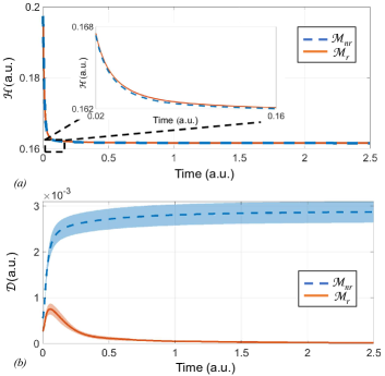
The optimal solution is reached when ϕi=±π2isubscriptitalic-ϕ𝑖plus-or-minus𝜋2for-all𝑖\phi_{i}=\pm\frac{\pi}{2}\enskip\forall i, which implies N=0subscript𝑁0\mathcal{L}_{N}=0. For the sake of comparison, we will consider two variants: (a) the non-resonant model (nrsubscript𝑛𝑟\mathcal{M}_{nr}) where β=0𝛽0\beta=0, and (b) the resonant model (rsubscript𝑟\mathcal{M}_{r}), where β0𝛽0\beta\neq 0. Figures 5(a) and (b) show a comparison of the cost Nsubscript𝑁\mathcal{H}_{N} and the regularization metric 𝒟Nsubscript𝒟𝑁\mathcal{D}_{N} (i=1N|Vi|2|Ii|2superscriptsubscript𝑖1𝑁superscriptsubscript𝑉𝑖2superscriptsubscript𝐼𝑖2\sum\limits_{i=1}^{N}\lvert V_{i}\rvert^{2}\lvert I_{i}\rvert^{2} for nrsubscript𝑛𝑟\mathcal{M}_{nr} and i=1N|Vi|2|Ii|2cos2ϕisuperscriptsubscript𝑖1𝑁superscriptsubscript𝑉𝑖2superscriptsubscript𝐼𝑖2superscript2subscriptitalic-ϕ𝑖\sum\limits_{i=1}^{N}\lvert V_{i}\rvert^{2}\lvert I_{i}\rvert^{2}\cos^{2}\phi_{i} for rsubscript𝑟\mathcal{M}_{r}), for N=5𝑁5N=5 and ω=π/10𝜔𝜋10\omega=\pi/10. In the case of nrsubscript𝑛𝑟\mathcal{M}_{nr}, N=Nsubscript𝑁subscript𝑁\mathcal{L}_{N}=\mathcal{H}_{N} and in the case of rsubscript𝑟\mathcal{M}_{r}, N=N+β𝒟Nsubscript𝑁subscript𝑁𝛽subscript𝒟𝑁\mathcal{L}_{N}=\mathcal{H}_{N}+\beta\mathcal{D}_{N}, with β=1𝛽1\beta=1. The solid line indicates the mean response across 101010 trials with random initializations of Vi,Iisubscript𝑉𝑖subscript𝐼𝑖V_{i},I_{i} and ϕisubscriptitalic-ϕ𝑖\phi_{i}. The shaded region shows the standard deviation across the trials in each case. Also shown in Figure 5(b) are the true active-power dissipation profiles (n=1N|Vi||Ii|superscriptsubscript𝑛1𝑁subscript𝑉𝑖subscript𝐼𝑖\sum\limits_{n=1}^{N}\lvert V_{i}\rvert\lvert I_{i}\rvert for nrsubscript𝑛𝑟\mathcal{M}_{nr} and n=1N|Vi||Ii|cosϕisuperscriptsubscript𝑛1𝑁subscript𝑉𝑖subscript𝐼𝑖subscriptitalic-ϕ𝑖\sum\limits_{n=1}^{N}\lvert V_{i}\rvert\lvert I_{i}\rvert\cos\phi_{i} for rsubscript𝑟\mathcal{M}_{r}) over the 10 trials.

It can be observed that under steady-state conditions, the model nrsubscript𝑛𝑟\mathcal{M}_{nr} dissipates power. However for the model rsubscript𝑟\mathcal{M}_{r} the steady-state active-power goes to zero. This is illustrated in Figure 5(b). Figure 5(c) shows the initial phasor configuration for the currents and voltages at each node of the network for a single trial for rsubscript𝑟\mathcal{M}_{r}. Here, we assume the voltage phasor Visubscript𝑉𝑖V_{i} to be aligned with the horizontal axis, and the current phasor Iisubscript𝐼𝑖I_{i} to be at an angle ϕisubscriptitalic-ϕ𝑖\phi_{i} with respect to the horizontal, ifor-all𝑖\forall i. Figure 5(d) shows the steady-state phasor configuration for rsubscript𝑟\mathcal{M}_{r} for the same trial. The voltage and current phasors are orthogonal to each other for all the nodes, thus verifying the zero active-power dissipation.

Refer to caption
Figure 5: Comparison of the resonant optimization model (rsubscript𝑟\mathcal{M}_{r}) with its non-resonant variant (nrsubscript𝑛𝑟\mathcal{M}_{nr}) for a quadratic objective function Nsubscript𝑁\mathcal{L}_{N} shown in Equation (19). For this experiment, N=5𝑁5N=5, input frequency ω=π/10𝜔𝜋10\omega=\pi/10, and the mean response is estimated over 10 trials with random initializations of Vi,Ii,ϕii=1,,5formulae-sequencesubscript𝑉𝑖subscript𝐼𝑖subscriptitalic-ϕ𝑖for-all𝑖15V_{i},I_{i},\phi_{i}\enskip\forall i=1,\ldots,5: (a) comparison of the time-evolution of Nsubscript𝑁\mathcal{H}_{N} for nrsubscript𝑛𝑟\mathcal{M}_{nr} and rsubscript𝑟\mathcal{M}_{r}, (b) comparison of the time-evolution of 𝒟Nsubscript𝒟𝑁\mathcal{D}_{N} (i=1N|Vi|2|Ii|2superscriptsubscript𝑖1𝑁superscriptsubscript𝑉𝑖2superscriptsubscript𝐼𝑖2\sum\limits_{i=1}^{N}\lvert V_{i}\rvert^{2}\lvert I_{i}\rvert^{2} for nrsubscript𝑛𝑟\mathcal{M}_{nr} and i=1N|Vi|2|Ii|2cos2ϕisuperscriptsubscript𝑖1𝑁superscriptsubscript𝑉𝑖2superscriptsubscript𝐼𝑖2superscript2subscriptitalic-ϕ𝑖\sum\limits_{i=1}^{N}\lvert V_{i}\rvert^{2}\lvert I_{i}\rvert^{2}\cos^{2}\phi_{i} for rsubscript𝑟\mathcal{M}_{r}). For all the curves, the line indicates the mean response, while the shaded region shows the standard deviation about the mean across the 10 trials. The true dissipation (n=1N|Vi||Ii|superscriptsubscript𝑛1𝑁subscript𝑉𝑖subscript𝐼𝑖\sum\limits_{n=1}^{N}\lvert V_{i}\rvert\lvert I_{i}\rvert for nrsubscript𝑛𝑟\mathcal{M}_{nr} and n=1N|Vi||Ii|cosϕisuperscriptsubscript𝑛1𝑁subscript𝑉𝑖subscript𝐼𝑖subscriptitalic-ϕ𝑖\sum\limits_{n=1}^{N}\lvert V_{i}\rvert\lvert I_{i}\rvert\cos\phi_{i} for rsubscript𝑟\mathcal{M}_{r}) over the 10 trials are also shown in the figure; Phasor representations of the LC tank voltages and currents for a single trial : (c) initial configuration and (d) final configuration for rsubscript𝑟\mathcal{M}_{r}. For rsubscript𝑟\mathcal{M}_{r}, β=1𝛽1\beta=1 for all the trials.

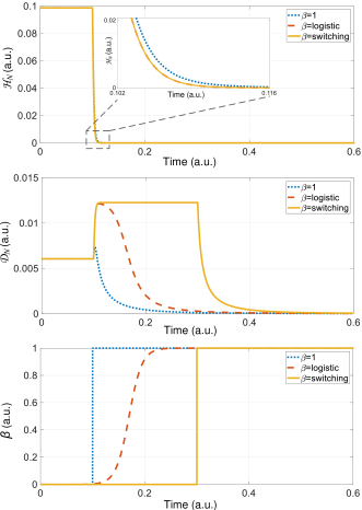
In the next set of experiments, we annealed the hyperparameter β𝛽\beta and evaluated its impact on the active-power dissipation metric 𝒟Nsubscript𝒟𝑁\mathcal{D}_{N} and the convergence of the object function Nsubscript𝑁\mathcal{H}_{N} for the model rsubscript𝑟\mathcal{M}_{r}. Figure 6 presents a comparison of the performance of rsubscript𝑟\mathcal{M}_{r} for different choices of annealing schedule for β𝛽\beta, with the angular frequency ω=π/10𝜔𝜋10\omega=\pi/10 as before. Figure 6(a) shows the time evolution of the objective function Nsubscript𝑁\mathcal{H}_{N}, 6(b) shows the time evolution of the dissipation metric 𝒟Nsubscript𝒟𝑁\mathcal{D}_{N} and 6(c) shows the annealing schedules adopted for β𝛽\beta. In all the cases, the optimization process starts after time t=0.1a.u.formulae-sequence𝑡0.1𝑎𝑢t=0.1\enskip a.u. from the onset of the simulation. The curves corresponding to β=1𝛽1\beta=1 denote the case when β𝛽\beta takes a constant value from t=0.1a.u.formulae-sequence𝑡0.1𝑎𝑢t=0.1\enskip a.u.; β=logistic𝛽logistic\beta=\text{logistic} corresponds to the case when β𝛽\beta is slowly increased from βmin=0subscript𝛽min0\beta_{\text{min}}=0 following a logistic curve of the form β(t)=βmin+βmaxβmin1+exp(k(t+t0))𝛽𝑡subscript𝛽minsubscript𝛽maxsubscript𝛽min1𝑘𝑡subscript𝑡0\beta(t)=\beta_{\text{min}}+\dfrac{\beta_{\text{max}}-\beta_{\text{min}}}{1+\exp(-k(t+t_{0}))} from t=0.1a.u.formulae-sequence𝑡0.1𝑎𝑢t=0.1\enskip a.u., and takes on a maximum value of βmax=1subscript𝛽max1\beta_{\text{max}}=1 (k𝑘k and t0subscript𝑡0t_{0} are hyperparameters determining the steepness and mid-point of the sigmoid respectively); β=switching𝛽switching\beta=\text{switching} corresponds to the case when β𝛽\beta switches from a minimum value (βmin=0subscript𝛽min0\beta_{\text{min}}=0) to a maximum value (βmax=1subscript𝛽max1\beta_{\text{max}}=1) at t=0.3a.u.formulae-sequence𝑡0.3𝑎𝑢t=0.3\enskip a.u., after the system has converged to the optimal solution. We can observe that in all of the cases, the model converges to the optimal solution, irrespective of the choice of β𝛽\beta. However, different annealing schedules for β𝛽\beta lead to different active-power dissipation profiles. For example, a constant value of β𝛽\beta throughout the duration of the experiment would lead to faster minimization of the active-power dissipation metric, but at the cost of slower convergence. The opposite trend can be seen when β𝛽\beta is slowly annealed to a sufficiently high value throughout the course of the optimization. The annealing schedule thus acts as a trade-off between the speed of convergence, and the rate of minimization of the active power.
Refer to caption
Figure 6: Comparison of the performance of the resonant model rsubscript𝑟\mathcal{M}_{r} for different choices of annealing schedule for β𝛽\beta (N=5,ω=π/10formulae-sequence𝑁5𝜔𝜋10N=5,\omega=\pi/10): (a) time evolution of Nsubscript𝑁\mathcal{H}_{N} (inset shows a zoomed in view of the cost evolution in the transient phase), (b) time evolution of 𝒟Nsubscript𝒟𝑁\mathcal{D}_{N} and (c) time evolution of β𝛽\beta. In all the cases, the optimization process starts after 0.1a.u.formulae-sequence0.1𝑎𝑢0.1\enskip a.u. from the onset of the simulation. The curves corresponding to β=1𝛽1\beta=1 denotes the case when β𝛽\beta takes a constant value from t=0.1a.u.formulae-sequence𝑡0.1𝑎𝑢t=0.1\enskip a.u.; β=logistic𝛽logistic\beta=\text{logistic} corresponds to the cases when β𝛽\beta is slowly increased following a logistic curve from t=0.1a.u.formulae-sequence𝑡0.1𝑎𝑢t=0.1\enskip a.u., and takes on a maximum value of β=1𝛽1\beta=1; β=switching𝛽switching\beta=\text{switching} corresponds to the case when β𝛽\beta switches from a minimum value(=0absent0=0) to a maximum value(=1absent1=1) at t=0.3a.u.formulae-sequence𝑡0.3𝑎𝑢t=0.3\enskip a.u., after the system has converged to the optimal solution.

IV-A Model Properties and Extensions

The dynamical system represented by Equations (15)-(18) and the resonant optimization framework also exhibits the following properties and extensions:

  1. 1.

    Energy constraints can be imposed over subgroups of nodes in the network: We can have the reactive energy conservation constraint between subgroups of nodes, instead of on the network as a whole, i.e., i=1Nk(|Vik|2+|Iik|2)=1k=1,,Mformulae-sequencesuperscriptsubscript𝑖1subscript𝑁𝑘superscriptsubscript𝑉𝑖𝑘2superscriptsubscript𝐼𝑖𝑘21for-all𝑘1𝑀\sum\limits_{i=1}^{N_{k}}\Big{(}\lvert V_{ik}\rvert^{2}+\lvert I_{ik}\rvert^{2}\Big{)}=1\enskip\forall k=1,\ldots,M. Here M=𝑀absentM=number of subgroups and Nk=subscript𝑁𝑘absentN_{k}= number of nodes in the kthsuperscript𝑘thk^{\text{th}} subgroup. The update equations in this case are given by:

    Vik(t)t=jωkσVik(t)Vik(t)ΔσVik(t)Vik(t)subscript𝑉𝑖𝑘𝑡𝑡𝑗subscript𝜔𝑘subscript𝜎subscript𝑉𝑖𝑘𝑡subscript𝑉𝑖𝑘𝑡Δsubscript𝜎subscript𝑉𝑖𝑘𝑡subscript𝑉𝑖𝑘𝑡\displaystyle\dfrac{\partial V_{ik}(t)}{\partial t}=j\omega_{k}\sigma_{V_{ik}}(t)V_{ik}(t)-\Delta\sigma_{V_{ik}}(t)V_{ik}(t)
    Iik(t)t=j(ωk+ωϕik)σIik(t)Iik(t)ΔσIik(t)Iik(t)subscript𝐼𝑖𝑘𝑡𝑡𝑗subscript𝜔𝑘subscript𝜔subscriptitalic-ϕ𝑖𝑘subscript𝜎subscript𝐼𝑖𝑘𝑡subscript𝐼𝑖𝑘𝑡Δsubscript𝜎subscript𝐼𝑖𝑘𝑡subscript𝐼𝑖𝑘𝑡\displaystyle\dfrac{\partial I_{ik}(t)}{\partial t}=j(\omega_{k}+\omega_{\phi_{ik}})\sigma_{I_{ik}}(t)I_{ik}(t)-\Delta\sigma_{I_{ik}}(t)I_{ik}(t)
    τikωϕik+ϕik(t)=gϕik(t)i,k,subscript𝜏𝑖𝑘subscript𝜔subscriptitalic-ϕ𝑖𝑘subscriptitalic-ϕ𝑖𝑘𝑡subscript𝑔subscriptitalic-ϕ𝑖𝑘𝑡for-all𝑖𝑘\displaystyle\tau_{ik}\omega_{\phi_{ik}}+\phi_{ik}(t)=g_{\phi_{ik}}(t)\quad\forall i,k, (21)

    where ωksubscript𝜔𝑘\omega_{k} is the constant angular frequency of the kthsuperscript𝑘thk^{\text{th}} subgroup of nodes, and ωϕik=dϕik(t)dtsubscript𝜔subscriptitalic-ϕ𝑖𝑘𝑑subscriptitalic-ϕ𝑖𝑘𝑡𝑑𝑡\omega_{\phi_{ik}}=\dfrac{d\phi_{ik}(t)}{dt}.

  2. 2.

    System dynamics and reactive-energy constraints remain invariant under the imposition of a global phase: The network dynamics remain invariant to the imposition of a global phase component on all the network variables, and the conservation constraint is also satisfied in this case. The governing equations are given by:

    Vi(t)tsubscript𝑉𝑖𝑡𝑡\displaystyle\dfrac{\partial V_{i}(t)}{\partial t} =j(ω+ωϕg)σVi(t)Vi(t)ΔσVi(t)Vi(t),absent𝑗𝜔subscript𝜔subscriptitalic-ϕ𝑔subscript𝜎subscript𝑉𝑖𝑡subscript𝑉𝑖𝑡Δsubscript𝜎subscript𝑉𝑖𝑡subscript𝑉𝑖𝑡\displaystyle=j(\omega+\omega_{\phi_{g}})\sigma_{V_{i}}(t)V_{i}(t)-\Delta\sigma_{V_{i}}(t)V_{i}(t),
    Ii(t)tsubscript𝐼𝑖𝑡𝑡\displaystyle\dfrac{\partial I_{i}(t)}{\partial t} =j(ω+ωϕg+ωϕi)σIi(t)Ii(t)ΔσIi(t)Ii(t),absent𝑗𝜔subscript𝜔subscriptitalic-ϕ𝑔subscript𝜔subscriptitalic-ϕ𝑖subscript𝜎subscript𝐼𝑖𝑡subscript𝐼𝑖𝑡Δsubscript𝜎subscript𝐼𝑖𝑡subscript𝐼𝑖𝑡\displaystyle=j(\omega+\omega_{\phi_{g}}+\omega_{\phi_{i}})\sigma_{I_{i}}(t)I_{i}(t)-\Delta\sigma_{I_{i}}(t)I_{i}(t), (22)

    where ϕgsubscriptitalic-ϕ𝑔\phi_{g} is the global phase and ωϕg=dϕgdtsubscript𝜔subscriptitalic-ϕ𝑔𝑑subscriptitalic-ϕ𝑔𝑑𝑡\omega_{\phi_{g}}=\dfrac{d\phi_{g}}{dt}.

  3. 3.

    Reactive-energy constraints remain invariant with varying network dynamics under the imposition of a relative phase: The conservation constraints are satisfied on the introduction of a relative phase component between the voltage and current phasors of each node, even though the overall network dynamics change. The governing equations are given by:

    Vi(t)tsubscript𝑉𝑖𝑡𝑡\displaystyle\dfrac{\partial V_{i}(t)}{\partial t} =j(ω+ωϕVi)σVi(t)Vi(t)ΔσVi(t)Vi(t),absent𝑗𝜔subscript𝜔subscriptitalic-ϕsubscript𝑉𝑖subscript𝜎subscript𝑉𝑖𝑡subscript𝑉𝑖𝑡Δsubscript𝜎subscript𝑉𝑖𝑡subscript𝑉𝑖𝑡\displaystyle=j(\omega+\omega_{\phi_{V_{i}}})\sigma_{V_{i}}(t)V_{i}(t)-\Delta\sigma_{V_{i}}(t)V_{i}(t),
    Ii(t)tsubscript𝐼𝑖𝑡𝑡\displaystyle\dfrac{\partial I_{i}(t)}{\partial t} =j(ω+ωϕIi+ωϕi)σIi(t)Ii(t)ΔσIi(t)Ii(t),absent𝑗𝜔subscript𝜔subscriptitalic-ϕsubscript𝐼𝑖subscript𝜔subscriptitalic-ϕ𝑖subscript𝜎subscript𝐼𝑖𝑡subscript𝐼𝑖𝑡Δsubscript𝜎subscript𝐼𝑖𝑡subscript𝐼𝑖𝑡\displaystyle=j(\omega+\omega_{\phi_{I_{i}}}+\omega_{\phi_{i}})\sigma_{I_{i}}(t)I_{i}(t)-\Delta\sigma_{I_{i}}(t)I_{i}(t), (23)

    where ϕi=ϕIiϕVisubscriptitalic-ϕ𝑖subscriptitalic-ϕsubscript𝐼𝑖subscriptitalic-ϕsubscript𝑉𝑖\phi_{i}=\phi_{I_{i}}-\phi_{V_{i}} is the relative external phase shift applied between the voltage and current phasors of the ithsuperscript𝑖thi^{\text{th}} node, ωϕVi=dϕVidtsubscript𝜔subscriptitalic-ϕsubscript𝑉𝑖𝑑subscriptitalic-ϕsubscript𝑉𝑖𝑑𝑡\omega_{\phi_{V_{i}}}=\dfrac{d\phi_{V_{i}}}{dt} and ωϕIi=dϕIidtsubscript𝜔subscriptitalic-ϕsubscript𝐼𝑖𝑑subscriptitalic-ϕsubscript𝐼𝑖𝑑𝑡\omega_{\phi_{I_{i}}}=\dfrac{d\phi_{I_{i}}}{dt}.

  4. 4.

    The model is dissipative and converges to limit cycle oscillations in steady state: The second order time derivatives of Equations (15) and (16) lead to the following:

    2Vit2=jωσViVi˙+jωViσVi˙ΔσViVi˙+σVi˙Visuperscript2subscript𝑉𝑖superscript𝑡2𝑗𝜔subscript𝜎subscript𝑉𝑖˙subscript𝑉𝑖𝑗𝜔subscript𝑉𝑖˙subscript𝜎subscript𝑉𝑖Δsubscript𝜎subscript𝑉𝑖˙subscript𝑉𝑖˙subscript𝜎subscript𝑉𝑖subscript𝑉𝑖\displaystyle\dfrac{\partial^{2}V_{i}}{\partial t^{2}}=j\omega\sigma_{V_{i}}\dot{V_{i}}+j\omega V_{i}\dot{\sigma_{V_{i}}}-\Delta\sigma_{V_{i}}\dot{V_{i}}+\dot{\sigma_{V_{i}}}V_{i}
    =ω2σVi2Vilimit cycles+absentlimit-fromsubscriptsuperscript𝜔2superscriptsubscript𝜎subscript𝑉𝑖2subscript𝑉𝑖limit cycles\displaystyle=\underbrace{-\omega^{2}\sigma_{V_{i}}^{2}V_{i}}_{\text{limit cycles}}+
    [1+jω]σ˙ViVi2jωσViΔσViVi+(ΔσVi)2Vidissipation,subscriptdelimited-[]1𝑗𝜔subscript˙𝜎subscript𝑉𝑖subscript𝑉𝑖2𝑗𝜔subscript𝜎subscript𝑉𝑖Δsubscript𝜎subscript𝑉𝑖subscript𝑉𝑖superscriptΔsubscript𝜎subscript𝑉𝑖2subscript𝑉𝑖dissipation\displaystyle\underbrace{[1+j\omega]\dot{\sigma}_{V_{i}}V_{i}-2j\omega\sigma_{V_{i}}\Delta\sigma_{V_{i}}V_{i}+(\Delta\sigma_{V_{i}})^{2}V_{i}}_{\text{dissipation}}, (24)
    2Iit2=jωϕiσIiIi˙+jωϕiIiσIi˙ΔσIiIi˙+σIi˙Iisuperscript2subscript𝐼𝑖superscript𝑡2𝑗subscriptsuperscript𝜔subscriptitalic-ϕ𝑖subscript𝜎subscript𝐼𝑖˙subscript𝐼𝑖𝑗subscriptsuperscript𝜔subscriptitalic-ϕ𝑖subscript𝐼𝑖˙subscript𝜎subscript𝐼𝑖Δsubscript𝜎subscript𝐼𝑖˙subscript𝐼𝑖˙subscript𝜎subscript𝐼𝑖subscript𝐼𝑖\displaystyle\dfrac{\partial^{2}I_{i}}{\partial t^{2}}=j\omega^{\prime}_{\phi_{i}}\sigma_{I_{i}}\dot{I_{i}}+j\omega^{\prime}_{\phi_{i}}I_{i}\dot{\sigma_{I_{i}}}-\Delta\sigma_{I_{i}}\dot{I_{i}}+\dot{\sigma_{I_{i}}}I_{i}
    =(ωϕi)2σIi2Iilimit cycles+absentlimit-fromsubscriptsuperscriptsubscriptsuperscript𝜔subscriptitalic-ϕ𝑖2superscriptsubscript𝜎subscript𝐼𝑖2subscript𝐼𝑖limit cycles\displaystyle=\underbrace{-(\omega^{\prime}_{\phi_{i}})^{2}\sigma_{I_{i}}^{2}I_{i}}_{\text{limit cycles}}+
    [1+jωϕi]σ˙IiIi2jωϕiσIiΔσIiIi+(ΔσIi)2Iidissipation,subscriptdelimited-[]1𝑗subscriptsuperscript𝜔subscriptitalic-ϕ𝑖subscript˙𝜎subscript𝐼𝑖subscript𝐼𝑖2𝑗subscriptsuperscript𝜔subscriptitalic-ϕ𝑖subscript𝜎subscript𝐼𝑖Δsubscript𝜎subscript𝐼𝑖subscript𝐼𝑖superscriptΔsubscript𝜎subscript𝐼𝑖2subscript𝐼𝑖dissipation\displaystyle\underbrace{[1+j\omega^{\prime}_{\phi_{i}}]\dot{\sigma}_{I_{i}}I_{i}-2j\omega^{\prime}_{\phi_{i}}\sigma_{I_{i}}\Delta\sigma_{I_{i}}I_{i}+(\Delta\sigma_{I_{i}})^{2}I_{i}}_{\text{dissipation}}, (25)

    where ωϕi=ω+ωϕisubscriptsuperscript𝜔subscriptitalic-ϕ𝑖𝜔subscript𝜔subscriptitalic-ϕ𝑖\omega^{\prime}_{\phi_{i}}=\omega+\omega_{\phi_{i}}. The first terms in the RHS of Equations (24) and (25) correspond to stable limit cycle oscillations of all the phasors, while the other terms correspond to the dissipative effects in the network. This demonstrates that the network as a whole is essentially a coupled dissipative system that is capable of self-sustained oscillations under steady-state. Each individual state variable describing the network thus returns to the same position in its respective limit cycle at regular intervals of time, even when subjected to small perturbations.
Refer to caption
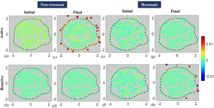
Figure 7: Comparison of the active and reactive power dissipated at each node for the non-resonant model nrsubscript𝑛𝑟\mathcal{M}_{nr} and the resonant model rsubscript𝑟\mathcal{M}_{r} for the synthetic one-class SVM problem on a two-dimensional dataset (Dataset I), with N=300,ν=0.1,ω=π/4formulae-sequence𝑁300formulae-sequence𝜈0.1𝜔𝜋4N=300,\nu=0.1,\omega=\pi/4, and random initializations for Vi,Ii,ϕii=1,,Nformulae-sequencesubscript𝑉𝑖subscript𝐼𝑖subscriptitalic-ϕ𝑖for-all𝑖1𝑁V_{i},I_{i},\phi_{i}\enskip\forall i=1,\ldots,N: (a), (c): the values of the active power metric (=|Vi||Ii|absentsubscript𝑉𝑖subscript𝐼𝑖=\lvert V_{i}\rvert\lvert I_{i}\rvert) at each node in the initial and final stages respectively for nrsubscript𝑛𝑟\mathcal{M}_{nr}; (b),(d): the values of the reactive power metric (=0absent0=0) at each node in the initial and final stages respectively for nrsubscript𝑛𝑟\mathcal{M}_{nr}; (e), (g): the values of the active power metric (=|Vi||Ii|cosϕiabsentsubscript𝑉𝑖subscript𝐼𝑖subscriptitalic-ϕ𝑖=\lvert V_{i}\rvert\lvert I_{i}\rvert\cos\phi_{i}) at each node in the initial and final stages respectively for rsubscript𝑟\mathcal{M}_{r}; (f), (h): the values of the reactive power metric (=|Vi||Ii|sinϕiabsentsubscript𝑉𝑖subscript𝐼𝑖subscriptitalic-ϕ𝑖=\lvert V_{i}\rvert\lvert I_{i}\rvert\sin\phi_{i}) at each node in the initial and final stages respectively for rsubscript𝑟\mathcal{M}_{r}. For both models, K(,)𝐾K(\cdot,\cdot) was chosen to be a Gaussian kernel with kernel parameter σ=1𝜎1\sigma=1, and β=1𝛽1\beta=1 throughout the optimization process for rsubscript𝑟\mathcal{M}_{r}.

V Resonant Machine Learning Framework

In this section, we show how the framework introduced in Section III can be applied for constructing resonant machine learning networks. In general, the framework can be applied to any learning network that optimizes a cost function defined over a set of learning variables αisubscript𝛼𝑖\alpha_{i} as

min{αi}({αi})+hΨ({αi})subscript𝛼𝑖minsubscript𝛼𝑖Ψsubscript𝛼𝑖\displaystyle\underset{\{\alpha_{i}\}}{\text{min}}\quad\mathcal{H}(\{\alpha_{i}\})+h\Psi(\{\alpha_{i}\})
s.t.i=1Nαi=1,αi0i=1,,N.formulae-sequences.t.superscriptsubscript𝑖1𝑁subscript𝛼𝑖1formulae-sequencesubscript𝛼𝑖0for-all𝑖1𝑁\displaystyle\textit{s.t.}\quad\sum_{i=1}^{N}\alpha_{i}=1,\quad\alpha_{i}\geq 0\quad\forall i=1,\ldots,N. (26)

Here ({αi})subscript𝛼𝑖\mathcal{H}(\{\alpha_{i}\}) represents a loss-function [28] which depends on the learning problem (e.g. supervised, unsupervised or semi-supervised) and the dataset under consideration (e.g., training data). The second term Ψ()Ψ\Psi(\cdot) in the objective function is any linear or nonlinear function which represents either (a) a regularization function, or (b) a penalty function used to satisfy optimization constraints. hh is a hyperparameter which acts as a trade-off between ()\mathcal{H}(\cdot) and Ψ()Ψ\Psi(\cdot). Because αisubscript𝛼𝑖\alpha_{i} could be viewed as probability measure, the optimization framework in Equation (26) naturally lends itself to probabilistic learning models [29, 30, 31].

The above problem can be mapped to the resonant learning framework in Section III by substituting αi=|Vi|2+|Ii|2subscript𝛼𝑖superscriptsubscript𝑉𝑖2superscriptsubscript𝐼𝑖2\alpha_{i}=\lvert V_{i}\rvert^{2}+\lvert I_{i}\rvert^{2}, to arrive at the following problem:

min{|Vi|,|Ii|,ϕi}({|Vi|,|Ii|})+hΨ({|Vi|,|Ii|})subscript𝑉𝑖subscript𝐼𝑖subscriptitalic-ϕ𝑖minsubscript𝑉𝑖subscript𝐼𝑖Ψsubscript𝑉𝑖subscript𝐼𝑖\displaystyle\underset{\{\lvert V_{i}\rvert,\lvert I_{i}\rvert,\phi_{i}\}}{\text{min}}\quad\mathcal{H}(\{\lvert V_{i}\rvert,\lvert I_{i}\rvert\})+h\Psi(\{\lvert V_{i}\rvert,\lvert I_{i}\rvert\})
+βi=1N|Vi|2|Ii|2cos2ϕi𝛽superscriptsubscript𝑖1𝑁superscriptsubscript𝑉𝑖2superscriptsubscript𝐼𝑖2superscript2subscriptitalic-ϕ𝑖\displaystyle+\beta\sum\limits_{i=1}^{N}\lvert V_{i}\rvert^{2}\lvert I_{i}\rvert^{2}\cos^{2}\phi_{i}
s.t.i=1N(|Vi|2+|Ii|2)=1,|ϕ|πi=1,,Nformulae-sequences.t.superscriptsubscript𝑖1𝑁superscriptsubscript𝑉𝑖2superscriptsubscript𝐼𝑖21formulae-sequenceitalic-ϕ𝜋for-all𝑖1𝑁\displaystyle\textit{s.t.}\quad\sum_{i=1}^{N}(\lvert V_{i}\rvert^{2}+\lvert I_{i}\rvert^{2})=1,\quad\lvert\phi\rvert\leq\pi\quad\forall i=1,\ldots,N (27)

Note that non-probabilistic learning problems can also be mapped to the probabilistic framework by imposing an additional constraint, as discussed in Appendix A.

V-A One-class resonant SVM

We now show how the framework in Equation (27) can be used to design a resonant one-class SVM.

The solution of a generic one-class SVM is obtained by solving the following optimization problem [8, 32, 33]:

min{αi}12i=1Nj=1NαiK(𝐱i,𝐱j)αjsubscript𝛼𝑖min12superscriptsubscript𝑖1𝑁superscriptsubscript𝑗1𝑁subscript𝛼𝑖𝐾subscript𝐱𝑖subscript𝐱𝑗subscript𝛼𝑗\displaystyle\underset{\{\alpha_{i}\}}{\text{min}}\quad\dfrac{1}{2}\sum\limits_{i=1}^{N}\sum\limits_{j=1}^{N}\alpha_{i}K({\mathbf{x}}_{i},{\mathbf{x}}_{j})\alpha_{j}
s.t.i=1Nαi=1,0<αi<1νNi=1,,Nformulae-sequences.t.superscriptsubscript𝑖1𝑁subscript𝛼𝑖10subscript𝛼𝑖1𝜈𝑁for-all𝑖1𝑁\displaystyle\textit{s.t.}\quad\sum_{i=1}^{N}\alpha_{i}=1,\quad 0<\alpha_{i}<\dfrac{1}{\nu N}\quad\forall i=1,\ldots,N (28)

where 𝐗=[𝐱𝟏,,𝐱𝐢,,𝐱𝐍]N×D𝐗subscript𝐱1subscript𝐱𝐢subscript𝐱𝐍superscript𝑁𝐷\mathbf{X}=[\mathbf{x_{1}},\ldots,\mathbf{x_{i}},\ldots,\mathbf{x_{N}}]\in\mathbb{R}^{N\times D} is the Dlimit-from𝐷D-dimensional input dataset of size N𝑁N, ν{0,1}𝜈01\nu\in\{0,1\} is a parameter which controls the size of the decision surface, K(,)𝐾K(\cdot,\cdot) is a positive definite Kernel function satisfying Mercer’s conditions, and αisubscript𝛼𝑖\alpha_{i}’s are the learning parameters. The optimization problem above can be reformulated by replacing the inequality constraint with a smooth penalty or loss function Ψ()Ψ\Psi(\cdot) like the logarithmic barrier, e.g., Ψ(αi,ν)=log(1νNαi)Ψsubscript𝛼𝑖𝜈1𝜈𝑁subscript𝛼𝑖\Psi(\alpha_{i},\nu)=-\log(\dfrac{1}{\nu N}-\alpha_{i}).

min{αi}=12i=1Nj=1NαiK(𝐱i,𝐱j)αj+hi=1NΨ(αi,ν)subscript𝛼𝑖min12superscriptsubscript𝑖1𝑁superscriptsubscript𝑗1𝑁subscript𝛼𝑖𝐾subscript𝐱𝑖subscript𝐱𝑗subscript𝛼𝑗superscriptsubscript𝑖1𝑁Ψsubscript𝛼𝑖𝜈\displaystyle\underset{\{\alpha_{i}\}}{\text{min}}\quad\mathcal{H}=\dfrac{1}{2}\sum\limits_{i=1}^{N}\sum\limits_{j=1}^{N}\alpha_{i}K({\mathbf{x}}_{i},{\mathbf{x}}_{j})\alpha_{j}\ +h\sum\limits_{i=1}^{N}\Psi(\alpha_{i},\nu)
s.t.i=1Nαi=1,s.t.superscriptsubscript𝑖1𝑁subscript𝛼𝑖1\displaystyle\textit{s.t.}\quad\sum_{i=1}^{N}\alpha_{i}=1, (29)

The parameter hh determines the steepness of the penalty function, where a lower value of hh implies an almost-accurate inequality constraint.
Refer to caption
Figure 8: Comparison of the performance of the resonant model rsubscript𝑟\mathcal{M}_{r} for different choices of annealing schedules for β𝛽\beta for the one-class SVM problem, on three different two-dimensional synthetic datasets for a simulation duration of t=4a.u.formulae-sequence𝑡4𝑎𝑢t=4\enskip a.u.. In all cases, N=300,ν=0.1,ω=π/20formulae-sequence𝑁300formulae-sequence𝜈0.1𝜔𝜋20N=300,\nu=0.1,\omega=\pi/20, and K(,)𝐾K(\cdot,\cdot) was chosen to be a Gaussian kernel with parameter values σ=1,10𝜎110\sigma=1,10 and 202020 for synthetic Dataset I, II and III respectively. Additionally for each dataset, Vi,Ii,ϕisubscript𝑉𝑖subscript𝐼𝑖subscriptitalic-ϕ𝑖V_{i},I_{i},\phi_{i} were randomly initialized i=1,,Nfor-all𝑖1𝑁\forall i=1,\ldots,N: (a) contour plot with the decision boundary around the datapoints and support vectors (SVs); (b) time evolution of \mathcal{H} (inset shows a zoomed in view of the cost evolution in the transient phase); (c) time evolution of 𝒟𝒟\mathcal{D} and (d) time evolution of β𝛽\beta for different annealing schedules. The curves corresponding to β=1𝛽1\beta=1 and 101010 denote the cases when β𝛽\beta takes a constant value throughout the simulation duration; β=logistic1𝛽subscriptlogistic1\beta=\text{logistic}_{1} and β=logistic2𝛽subscriptlogistic2\beta=\text{logistic}_{2} correspond to the cases when β𝛽\beta is slowly increased following a logistic curve, and takes on maximum values of βmax=1subscript𝛽max1\beta_{\text{max}}=1 and βmax=10subscript𝛽max10\beta_{\text{max}}=10 respectively; β=switching𝛽switching\beta=\text{switching} corresponds to the case when β𝛽\beta switches from a minimum value(βmin=0subscript𝛽min0\beta_{\text{min}}=0) to a maximum value(βmax=10subscript𝛽max10\beta_{\text{max}}=10) at t=2a.u.formulae-sequence𝑡2𝑎𝑢t=2\enskip a.u., after the system has converged to the optimal solution. (e)-(h) show similar plots on Dataset II, while (i)-(l) show the plots corresponding to Dataset III.
Refer to caption
Figure 9: Robustness to random initialization: Comparison of (a) the time-evolution of the cost \mathcal{H} and (b) the dissipation metric profile 𝒟𝒟\mathcal{D} (n=1N|Vi|2|Ii|2superscriptsubscript𝑛1𝑁superscriptsubscript𝑉𝑖2superscriptsubscript𝐼𝑖2\sum\limits_{n=1}^{N}\lvert V_{i}\rvert^{2}\lvert I_{i}\rvert^{2} for the non-resonant model nrsubscript𝑛𝑟\mathcal{M}_{nr} and n=1N|Vi|2|Ii|2cos2ϕisuperscriptsubscript𝑛1𝑁superscriptsubscript𝑉𝑖2superscriptsubscript𝐼𝑖2superscript2subscriptitalic-ϕ𝑖\sum\limits_{n=1}^{N}\lvert V_{i}\rvert^{2}\lvert I_{i}\rvert^{2}\cos^{2}\phi_{i} for the resonant model rsubscript𝑟\mathcal{M}_{r} respectively) for the synthetic one-class SVM problem on Dataset I for N=300,ν=0.1,ω=π/8formulae-sequence𝑁300formulae-sequence𝜈0.1𝜔𝜋8N=300,\nu=0.1,\omega=\pi/8 over 10 random initializations for Vi,Ii,ϕii=1,,Nformulae-sequencesubscript𝑉𝑖subscript𝐼𝑖subscriptitalic-ϕ𝑖for-all𝑖1𝑁V_{i},I_{i},\phi_{i}\enskip\forall i=1,\ldots,N. The regularization parameter was chosen to be β=1𝛽1\beta=1 for the entire simulation duration of t=4a.u.formulae-sequence𝑡4𝑎𝑢t=4\enskip a.u. of the optimization process for rsubscript𝑟\mathcal{M}_{r}. For all the curves, the solid line indicates the mean response, while the shaded region shows the standard deviation about the mean across the trials.

An equivalent complex-domain representation in terms of voltages and currents in an LC network can be arrived at if we consider αi=|Vi|2+|Ii|2isubscript𝛼𝑖superscriptsubscript𝑉𝑖2superscriptsubscript𝐼𝑖2for-all𝑖\alpha_{i}=\lvert V_{i}\rvert^{2}+\lvert I_{i}\rvert^{2}\enskip\forall i. In this case, we consider that the network is globally energy constrained, and all the individual units in the network have the same frequency ω𝜔\omega. The redefined learning problem is as follows:

min{|Vi|,|Ii|}=12i=1Nj=1N(|Vi|2+|Ii|2)K(𝐱i,𝐱j)subscript𝑉𝑖subscript𝐼𝑖min12superscriptsubscript𝑖1𝑁superscriptsubscript𝑗1𝑁superscriptsubscript𝑉𝑖2superscriptsubscript𝐼𝑖2𝐾subscript𝐱𝑖subscript𝐱𝑗\displaystyle\underset{\{\lvert V_{i}\rvert,\lvert I_{i}\rvert\}}{\text{min}}\quad\mathcal{H}=\dfrac{1}{2}\sum\limits_{i=1}^{N}\sum\limits_{j=1}^{N}(\lvert V_{i}\rvert^{2}+\lvert I_{i}\rvert^{2})K({\mathbf{x}}_{i},{\mathbf{x}}_{j})
×(|Vj|2+|Ij|2)+hi=1NΨ(|Vi|,|Ii|,ν)absentsuperscriptsubscript𝑉𝑗2superscriptsubscript𝐼𝑗2superscriptsubscript𝑖1𝑁Ψsubscript𝑉𝑖subscript𝐼𝑖𝜈\displaystyle\times(\lvert V_{j}\rvert^{2}+\lvert I_{j}\rvert^{2})+h\sum\limits_{i=1}^{N}\Psi(\lvert V_{i}\rvert,\lvert I_{i}\rvert,\nu)
s.t.i=1N(|Vi|2+|Ii|2)=1.s.t.superscriptsubscript𝑖1𝑁superscriptsubscript𝑉𝑖2superscriptsubscript𝐼𝑖21\displaystyle\textit{s.t.}\quad\sum_{i=1}^{N}(\lvert V_{i}\rvert^{2}+\lvert I_{i}\rvert^{2})=1. (30)

Introducing the active-power dissipation regularization we arrive at the following problem:

min{|Vi|,|Ii|,ϕi}=12i=1Nj=1N(|Vi|2+|Ii|2)K(𝐱i,𝐱j)subscript𝑉𝑖subscript𝐼𝑖subscriptitalic-ϕ𝑖min12superscriptsubscript𝑖1𝑁superscriptsubscript𝑗1𝑁superscriptsubscript𝑉𝑖2superscriptsubscript𝐼𝑖2𝐾subscript𝐱𝑖subscript𝐱𝑗\displaystyle\underset{\{\lvert V_{i}\rvert,\lvert I_{i}\rvert,\phi_{i}\}}{\text{min}}\quad\mathcal{L}=\dfrac{1}{2}\sum\limits_{i=1}^{N}\sum\limits_{j=1}^{N}(\lvert V_{i}\rvert^{2}+\lvert I_{i}\rvert^{2})K({\mathbf{x}}_{i},{\mathbf{x}}_{j})
×(|Vj|2+|Ij|2)+hi=1NΨ(|Vi|,|Ii|,ν)absentsuperscriptsubscript𝑉𝑗2superscriptsubscript𝐼𝑗2superscriptsubscript𝑖1𝑁Ψsubscript𝑉𝑖subscript𝐼𝑖𝜈\displaystyle\times(\lvert V_{j}\rvert^{2}+\lvert I_{j}\rvert^{2})+h\sum\limits_{i=1}^{N}\Psi(\lvert V_{i}\rvert,\lvert I_{i}\rvert,\nu)
+βi=1N|Vi|2|Ii|2cos2ϕi𝛽superscriptsubscript𝑖1𝑁superscriptsubscript𝑉𝑖2superscriptsubscript𝐼𝑖2superscript2subscriptitalic-ϕ𝑖\displaystyle+\beta\sum\limits_{i=1}^{N}\lvert V_{i}\rvert^{2}\lvert I_{i}\rvert^{2}\cos^{2}\phi_{i}
s.t.i=1N(|Vi|2+|Ii|2)=1,|ϕi|πi.formulae-sequences.t.superscriptsubscript𝑖1𝑁superscriptsubscript𝑉𝑖2superscriptsubscript𝐼𝑖21subscriptitalic-ϕ𝑖𝜋for-all𝑖\displaystyle\textit{s.t.}\quad\sum_{i=1}^{N}(\lvert V_{i}\rvert^{2}+\lvert I_{i}\rvert^{2})=1,\quad\lvert\phi_{i}\rvert\leq\pi\enskip\forall i. (31)

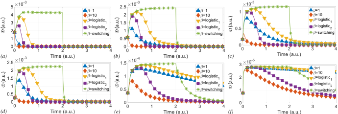
The update equations in this case are of the form shown in Equations (15)-(18). Figure 7 shows a comparison of the active and reactive power metrics of each node of the non-resonant model nrsubscript𝑛𝑟\mathcal{M}_{nr} and the resonant model rsubscript𝑟\mathcal{M}_{r} for a synthetic one-class SVM problem on a two-dimensional dataset (Dataset I). The dataset was generated by uniformly selecting 300300300 random points within a circle having a fixed radius. Here N=300,ν=0.1,ω=π/4formulae-sequence𝑁300formulae-sequence𝜈0.1𝜔𝜋4N=300,\nu=0.1,\omega=\pi/4, with random initializations for Vi,Ii,ϕii=1,,Nformulae-sequencesubscript𝑉𝑖subscript𝐼𝑖subscriptitalic-ϕ𝑖for-all𝑖1𝑁V_{i},I_{i},\phi_{i}\enskip\forall i=1,\ldots,N. A constant value of the regularization hyperparameter β=1𝛽1\beta=1 was considered throughout the duration of the optimization process for rsubscript𝑟\mathcal{M}_{r}. Figures 7(a) and (c) show the values of the active power metric (=|Vi||Ii|absentsubscript𝑉𝑖subscript𝐼𝑖=\lvert V_{i}\rvert\lvert I_{i}\rvert) at each node in the initial and final stages respectively for nrsubscript𝑛𝑟\mathcal{M}_{nr}, while Figures 7(b) and (d) show the values of the reactive power metric (=0absent0=0) at each node in the initial and final stages respectively for nrsubscript𝑛𝑟\mathcal{M}_{nr}. Similarly, Figures 7(e) and (g) show the values of the active power metric (=|Vi||Ii|cosϕiabsentsubscript𝑉𝑖subscript𝐼𝑖subscriptitalic-ϕ𝑖=\lvert V_{i}\rvert\lvert I_{i}\rvert\cos\phi_{i}) at each node in the initial and final stages respectively for rsubscript𝑟\mathcal{M}_{r} while Figures 7(f) and (h), finally, show the values of the reactive power metric (=|Vi||Ii|sinϕiabsentsubscript𝑉𝑖subscript𝐼𝑖subscriptitalic-ϕ𝑖=\lvert V_{i}\rvert\lvert I_{i}\rvert\sin\phi_{i}) at each node in the initial and final stages respectively for rsubscript𝑟\mathcal{M}_{r}.

Figure 8 shows a comparison of the performance of the resonant model rsubscript𝑟\mathcal{M}_{r} for different choices of annealing schedules for β𝛽\beta on three different two-dimensional synthetic datasets for a simulation duration of t=4a.u.formulae-sequence𝑡4𝑎𝑢t=4\enskip a.u.. In all cases, N=300,ν=0.1,ω=π/20formulae-sequence𝑁300formulae-sequence𝜈0.1𝜔𝜋20N=300,\nu=0.1,\omega=\pi/20, and K(,)𝐾K(\cdot,\cdot) was chosen to be a Gaussian kernel with parameter values σ=1,10𝜎110\sigma=1,10 and 202020 respectively for synthetic Dataset I, II and III. Additionally for each dataset, Vi,Ii,ϕisubscript𝑉𝑖subscript𝐼𝑖subscriptitalic-ϕ𝑖V_{i},I_{i},\phi_{i} were randomly initialized i=1,,Nfor-all𝑖1𝑁\forall i=1,\ldots,N. Figure 8(a) shows the contour plot with the decision boundary around the datapoints, along with the support vectors (SVs) for Dataset I, while Figures 8(b), (c) and (d) show the time evolutions of the cost \mathcal{H}, the dissipation metric 𝒟𝒟\mathcal{D} and the hyperparameter β𝛽\beta for different annealing schedules. The curves corresponding to β=1𝛽1\beta=1 and 101010 denote the cases when β𝛽\beta takes a constant value throughout the simulation duration. β=logistic1𝛽subscriptlogistic1\beta=\text{logistic}_{1} and β=logistic2𝛽subscriptlogistic2\beta=\text{logistic}_{2} correspond to the cases when β𝛽\beta is slowly increased following a logistic curve of the form β(t)=βmin+βmaxβmin1+exp(k(t+t0))𝛽𝑡subscript𝛽minsubscript𝛽maxsubscript𝛽min1𝑘𝑡subscript𝑡0\beta(t)=\beta_{\text{min}}+\dfrac{\beta_{\text{max}}-\beta_{\text{min}}}{1+\exp(-k(t+t_{0}))}, and takes on maximum values of βmax=1subscript𝛽max1\beta_{\text{max}}=1 and βmax=10subscript𝛽max10\beta_{\text{max}}=10 respectively starting from βmin=0subscript𝛽min0\beta_{\text{min}}=0. Finally, β=switching𝛽switching\beta=\text{switching} corresponds to the case when β𝛽\beta switches from a minimum value (βmin=0subscript𝛽min0\beta_{\text{min}}=0) to a maximum value (βmax=10subscript𝛽max10\beta_{\text{max}}=10) at t=2a.u.formulae-sequence𝑡2𝑎𝑢t=2\enskip a.u., after the system has converged to the optimal solution. Figures 8(e)-(h) show similar plots on Dataset II, while Figures 8(i)-(l) show the plots corresponding to Dataset III. Dataset I, as described before, was generated by selecting 300300300 points uniformly within a two-dimensional circle having a fixed radius. Datasets II and III also consist of 300300300 data points generated using a Gaussian mixture model consisting of four different clusters, with a fixed cluster mean and variance associated with each cluster. Dataset II and III differ only in terms of the cluster means associated with their respective constituent clusters, while the cluster variances are the same for all the clusters for both the datasets. It can be seen that since the optimization problem is convex, the model always converges to the optimal solution for every dataset, irrespective of the the annealing schedule for β𝛽\beta or the dataset complexity. However, the dissipation profiles corresponding to a particular annealing schedule strongly depend on the complexity of the dataset. In general, however, higher values of β𝛽\beta would lead to lower dissipation profiles during the learning process. Also, the model shows a much slower convergence in terms of the actual objective function for a constant non-zero value of β𝛽\beta throughout the optimization compared to the case when β𝛽\beta is slowly annealed to a sufficiently high value. The choice of a proper annealing schedule for β𝛽\beta would thus involve a trade-off between the speed of convergence and the rate of power dissipation.

Figures 9(a) and (b) finally, show the robustness of the proposed framework to different initial conditions by providing a comparison of the time evolutions of the cost \mathcal{H} and the dissipation metric 𝒟𝒟\mathcal{D} (n=1N|Vi|2|Ii|2superscriptsubscript𝑛1𝑁superscriptsubscript𝑉𝑖2superscriptsubscript𝐼𝑖2\sum\limits_{n=1}^{N}\lvert V_{i}\rvert^{2}\lvert I_{i}\rvert^{2} for the non-resonant model nrsubscript𝑛𝑟\mathcal{M}_{nr} and n=1N|Vi|2|Ii|2cos2ϕisuperscriptsubscript𝑛1𝑁superscriptsubscript𝑉𝑖2superscriptsubscript𝐼𝑖2superscript2subscriptitalic-ϕ𝑖\sum\limits_{n=1}^{N}\lvert V_{i}\rvert^{2}\lvert I_{i}\rvert^{2}\cos^{2}\phi_{i} for the resonant model rsubscript𝑟\mathcal{M}_{r} respectively), when applied to Dataset I. We show the results for 10 random initializations of Vi,Iisubscript𝑉𝑖subscript𝐼𝑖V_{i},I_{i} and ϕi,isubscriptitalic-ϕ𝑖for-all𝑖\phi_{i},\enskip\forall i. In all cases, ν=0.1,ω=π/8formulae-sequence𝜈0.1𝜔𝜋8\nu=0.1,\omega=\pi/8, and K(,)𝐾K(\cdot,\cdot) was chosen to be a Gaussian kernel with parameter value σ=1𝜎1\sigma=1. Note that even though the 10 trails had different initializations of Vi,Iisubscript𝑉𝑖subscript𝐼𝑖V_{i},I_{i}, they were chosen to have the same initial value of αisuperscriptsubscript𝛼𝑖\alpha_{i}^{\prime}s in all cases, because of which there is no deviation between the cost evolution curves for both nrsubscript𝑛𝑟\mathcal{M}_{nr} and rsubscript𝑟\mathcal{M}_{r}. The dissipation evolution is however different across different trials for both the models. However, the dissipation attains a final value of zero for rsubscript𝑟\mathcal{M}_{r} for all the trials, while there is a finite dissipation for nrsubscript𝑛𝑟\mathcal{M}_{nr} in all cases.

TABLE 2: Performance on real benchmark datasets for ν=0.1𝜈0.1\nu=0.1
Dataset Majority Class Size Correct Outliers SVs
Iris (50,4) 48 2 8
Heart (139,13) 1210 18 56
Diabetes (500,4) 466 34 90
Ecoli (327,7) 309 18 42
Adulta3a (2412,123) 2111 301 356
Mammography (10923,6) 9608 1315 5969
Refer to caption
Figure 10: Comparison of the dissipation profiles of the resonant model rsubscript𝑟\mathcal{M}_{r} for different choices of annealing schedules for β𝛽\beta for different real-life benchmark datasets :(a) ‘Iris’; (b) ‘Heart’; (c) ‘Diabetes; (d) ‘Ecoli’; (e) ‘Adulta3a’; and (f) ‘Mammography’.

We also conducted experiments on real-life benchmark datasets of varying sizes and dimensionality, considering the majority class as inliers in all cases. In all the experiments, we used similar parameter settings and annealing schedules as used in the experiments shown in Figure 8, and ν=0.1𝜈0.1\nu=0.1. Table 2 shows the dataset description along with the performance (number of inliers, number of outliers and number of support vectors) of the one-class SVM classifier for the following datasets: ‘Iris’ (inlier: class ‘setosa’), ‘Heart’ (inlier: ‘healthy’ heart), ‘Diabetes’ (inlier: non-diabetic patients), ‘Ecoli’ (inlier: classes ‘cp’, ‘im’, ‘pp’, ‘imU’ and ‘om’), ‘Adulta3a’ (inlier: individuals with income$50Kabsentcurrency-dollar50𝐾\leq\$50K) and ‘Mammography’ (inlier: non-calcifications)[34, 35]. Figures 10 (a)-(f) show the dissipation profiles corresponding to different annealing schedules for the different datasets. It can be seen that an optimal choice of the annealing schedule depends on both the dataset size and complexity, even though the dissipation decreases over time for all the cases, irrespective of the schedule chosen.

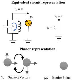
Interestingly, the solution of the one-class SVM can be interpreted in terms of an electrical network as follows, as shown in Figure 11: (a) the support vectors have voltage and current magnitudes with a ±π/2plus-or-minus𝜋2\pm\pi/2 phase shift between them, hence can be interpreted as resonant LC tanks; and (b) the interior points well inside the boundary have both zero voltage and current magnitudes, and can be essentially treated as floating sinks.

VI Discussions and Conclusions

In this paper we proposed a complex-domain formulation of a machine learning network that ensures that the network’s active power is dissipated only during the process of learning whereas the network’s reactive power is maintained to be zero at all times. We showed that the active power dissipation during learning can be controlled using a phase regularization parameter. Also, the framework is robust to variations in the initial conditions and to the choice of the input/driving frequency ω𝜔\omega. The proposed approach thus provides a physical interpretation of machine learning algorithms, where the energy required for storing learned parameters is sustained by electrical resonances due to nodal inductances and nodal capacitances. Using the one-class support vector machine problem as a case study, we have shown how the steady state solution of a learning problem can be interpreted in terms of these nodal circuit elements.
Refer to caption
Figure 11: Circuit based and phasor based representations for a one-class SVM problem: (a) support vectors, corresponding to resonant LC tanks and (b) interior points, corresponding to sinks/ground (Vi,Ii=0subscript𝑉𝑖subscript𝐼𝑖0V_{i},I_{i}=0).

Future directions involve exploring the implications of incorporating network dynamics in the free frequency variable ω𝜔\omega, and utilizing the phase information associated with each node in the learning process. Also, the experimental results presented in this paper were based on an unsupervised learning setting. Exploring an energy-efficient framework for supervised learning problems would also be a part of our future work.

In this paper we also proposed a dynamical system model based on complex-domain growth transforms. The formulation is general enough to be applicable to other complex-domain learning models[19, 20, 21, 22, 23]. Our proposed framework also preserves both the magnitude and phase information, and provides additional flexibilty compared to other complex domain learning models in terms of phase manipulation/cancellation [20].

In addition to implementing classic machine learning algorithms, the complex growth transform dynamical system can also be used for designing synchronized networks of coupled oscillators. Such networks can be potentially used for solving different computing tasks like optimization, pattern matching etc. as is achievable using coupled oscillatory computing models[36, 37]. An oscillator network designed in this fashion is capable of demonstrating stable, self-sustaining oscillatory dynamics, whereby the network can return to its initial stable limit cycle configuration following small perturbations, while simultaneously minimizing some underlying system-level objective function. The framework could also be used to study connections between learning and synchronization, or the emergence of a rhythmic periodic pattern exhibited by a group of coupled oscillators, which provides the key to understanding periodic processes pervading complex networks of different biological, physical, social and quantum ensembles [9, 38]. In this regard, the existing mathematical models for such collective behavior are mostly phenomenological or bottom-up, and in general do not provide a network-level perspective of the underlying physical process. The proposed growth-transform formulation, thus, could provide new network-level insights into the emergence of phase synchronization, phase cohesiveness and frequency synchronization in coupled-oscillator networks.

Note here that since we are implicitly assuming an analog implementation, the learning network should converge to the steady-state solution of the optimization, where the time of convergence depends on the network’s time-constant [39]. Hence the notion of time complexity is not well-defined. However, in a digital implementation, the time complexity would depend on the learning algorithm under consideration, dataset size and dimensionality, angular frequency ω𝜔\omega, and time constants τisubscript𝜏𝑖\tau_{i} for the phase updates.

VII Appendix

VII-A Resonance in an LC tank
Refer to caption
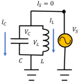
Figure 12: LC tank resonator

Consider the parallel LC tank circuit shown in Figure 12, with VCsubscript𝑉𝐶V_{C} and VLsubscript𝑉𝐿V_{L} being the voltages across the capacitor C𝐶C and inductor L𝐿L respectively. ICsubscript𝐼𝐶I_{C} and ILsubscript𝐼𝐿I_{L} denote the corresponding currents flowing through the elements. Thus, VS=VL=VCsubscript𝑉𝑆subscript𝑉𝐿subscript𝑉𝐶V_{S}=V_{L}=V_{C} and IS=IL+ICsubscript𝐼𝑆subscript𝐼𝐿subscript𝐼𝐶I_{S}=I_{L}+I_{C}. Considering the LC tank to be driven by the voltage source VSsubscript𝑉𝑆V_{S} at frequency ω𝜔\omega, we have the following condition in steady state:

IS(ω)=VS(ω)jωL[1ω2LC]subscript𝐼𝑆𝜔subscript𝑉𝑆𝜔𝑗𝜔𝐿delimited-[]1superscript𝜔2𝐿𝐶I_{S}(\omega)=\dfrac{V_{S}(\omega)}{j\omega L}[1-\omega^{2}LC] (32)

Resonant condition of the circuit is achieved when

ω=1LCIS(ω)=0𝜔1𝐿𝐶subscript𝐼𝑆𝜔0\displaystyle\omega=\dfrac{1}{\sqrt{LC}}\implies I_{S}(\omega)=0 (33)

This implies that the apparent power SN=PN+jQN=VSIS+VLIL+VCICsubscript𝑆𝑁subscript𝑃𝑁𝑗subscript𝑄𝑁subscript𝑉𝑆superscriptsubscript𝐼𝑆subscript𝑉𝐿superscriptsubscript𝐼𝐿subscript𝑉𝐶superscriptsubscript𝐼𝐶S_{N}=P_{N}+jQ_{N}=V_{S}I_{S}^{*}+V_{L}I_{L}^{*}+V_{C}I_{C}^{*}, where the active power PN=0subscript𝑃𝑁0P_{N}=0. Additionally at resonance, the reactive power QN=QC+QL=VLIL+VCIC=jωL|V(ω)|2+jωL|V(ω)|2=0subscript𝑄𝑁subscript𝑄𝐶subscript𝑄𝐿subscript𝑉𝐿superscriptsubscript𝐼𝐿subscript𝑉𝐶superscriptsubscript𝐼𝐶𝑗𝜔𝐿superscript𝑉𝜔2𝑗𝜔𝐿superscript𝑉𝜔20Q_{N}=Q_{C}+Q_{L}=V_{L}I_{L}^{*}+V_{C}I_{C}^{*}=-\dfrac{j}{\omega L}\lvert V(\omega)\rvert^{2}+\dfrac{j}{\omega L}\lvert V(\omega)\rvert^{2}=0. Here QCsubscript𝑄𝐶Q_{C} and QLsubscript𝑄𝐿Q_{L} are the reactive powers associated with the capacitance and inductance respectively.

VII-B Mapping a generic optimization problem to the equivalent network model

Let us consider an optimization problem defined over a probabilistic domain, given by the following generic form:

min{xi}({xi})subscript𝑥𝑖minsubscript𝑥𝑖\displaystyle\underset{\{x_{i}\}}{\text{min}}\quad\mathcal{H}(\{x_{i}\})
s.t.i=1Nxi=1,xi0formulae-sequences.t.superscriptsubscript𝑖1𝑁subscript𝑥𝑖1subscript𝑥𝑖0\displaystyle\textit{s.t.}\quad\sum_{i=1}^{N}x_{i}=1,\enskip x_{i}\geq 0 (34)

We can map the above to the electrical network-based model introduced in Section III by replacing xi=|Vi|2+|Ii|2subscript𝑥𝑖superscriptsubscript𝑉𝑖2superscriptsubscript𝐼𝑖2x_{i}=\lvert V_{i}\rvert^{2}+\lvert I_{i}\rvert^{2}, which leads to the following problem in the {|Vi|2,|Ii|2}superscriptsubscript𝑉𝑖2superscriptsubscript𝐼𝑖2\{\lvert V_{i}\rvert^{2},\lvert I_{i}\rvert^{2}\} domain:

min{|Vi|,|Ii|}({|Vi|,|Ii|})subscript𝑉𝑖subscript𝐼𝑖minsubscript𝑉𝑖subscript𝐼𝑖\displaystyle\underset{\{\lvert V_{i}\rvert,\lvert I_{i}\rvert\}}{\text{min}}\quad\mathcal{H}(\{\lvert V_{i}\rvert,\lvert I_{i}\rvert\})
s.t.i=1N(|Vi|2+|Ii|2)=1.s.t.superscriptsubscript𝑖1𝑁superscriptsubscript𝑉𝑖2superscriptsubscript𝐼𝑖21\displaystyle\textit{s.t.}\quad\sum_{i=1}^{N}\Big{(}\lvert V_{i}\rvert^{2}+\lvert I_{i}\rvert^{2}\Big{)}=1. (35)

Note that the method also works for optimization problems defined over non-probabilistic domains, of the following form:

min{xi}({xi})subscript𝑥𝑖minsubscript𝑥𝑖\displaystyle\underset{\{x_{i}\}}{\text{min}}\quad\mathcal{H}(\{x_{i}\})
s.t.|xi|1,xii=1,,N.formulae-sequenceformulae-sequences.t.subscript𝑥𝑖1subscript𝑥𝑖for-all𝑖1𝑁\displaystyle\textit{s.t.}\enskip\lvert x_{i}\rvert\leq 1,\enskip x_{i}\in\mathbb{R}\enskip\forall i=1,\ldots,N. (36)

This can be done by considering xi=xi+xiisubscript𝑥𝑖superscriptsubscript𝑥𝑖superscriptsubscript𝑥𝑖for-all𝑖x_{i}=x_{i}^{+}-x_{i}^{-}\enskip\forall i, where both xi+,xi0superscriptsubscript𝑥𝑖superscriptsubscript𝑥𝑖0x_{i}^{+},x_{i}^{-}\geq 0. Since by triangle inequality, |xi||xi+|+|xi|subscript𝑥𝑖superscriptsubscript𝑥𝑖superscriptsubscript𝑥𝑖\lvert x_{i}\rvert\leq\lvert x_{i}^{+}\rvert+\lvert x_{i}^{-}\rvert, enforcing xi++xi=1isuperscriptsubscript𝑥𝑖superscriptsubscript𝑥𝑖1for-all𝑖x_{i}^{+}+x_{i}^{-}=1\enskip\forall i would automatically ensure |xi|1isubscript𝑥𝑖1for-all𝑖\lvert x_{i}\rvert\leq 1\enskip\forall i. Thus we have,

argmin{xi}({xi})subscript𝑥𝑖argminsubscript𝑥𝑖\displaystyle\underset{\{x_{i}\}}{\text{argmin}}\quad\mathcal{H}(\{x_{i}\}) argmin{xi+,xi}({xi+,xi})absentsuperscriptsubscript𝑥𝑖superscriptsubscript𝑥𝑖argminsuperscriptsubscript𝑥𝑖superscriptsubscript𝑥𝑖\displaystyle\equiv\underset{\{x_{i}^{+},x_{i}^{-}\}}{\text{argmin}}\quad\mathcal{H}(\{x_{i}^{+},x_{i}^{-}\}) (37)
s.t.|xi|1,xiformulae-sequences.t.subscript𝑥𝑖1subscript𝑥𝑖\displaystyle\textit{s.t.}\quad\lvert x_{i}\rvert\leq 1,\enskip x_{i}\in\mathbb{R} s.t.xi++xi=1,xi+,xi0formulae-sequences.t.superscriptsubscript𝑥𝑖superscriptsubscript𝑥𝑖1superscriptsubscript𝑥𝑖superscriptsubscript𝑥𝑖0\displaystyle\quad\quad\textit{s.t.}\quad x_{i}^{+}+x_{i}^{-}=1,\enskip x_{i}^{+},x_{i}^{-}\geq 0

In this case, we replace xi+=|Vi|2,xi=|Ii|2formulae-sequencesuperscriptsubscript𝑥𝑖superscriptsubscript𝑉𝑖2superscriptsubscript𝑥𝑖superscriptsubscript𝐼𝑖2x_{i}^{+}=\lvert V_{i}\rvert^{2},\enskip x_{i}^{-}=\lvert I_{i}\rvert^{2}, and the equivalent problem in the {|Vi|2,|Ii|2}superscriptsubscript𝑉𝑖2superscriptsubscript𝐼𝑖2\{\lvert V_{i}\rvert^{2},\lvert I_{i}\rvert^{2}\} domain is thus as follows:

min{|Vi|,|Ii|}({|Vi|,|Ii|})subscript𝑉𝑖subscript𝐼𝑖minsubscript𝑉𝑖subscript𝐼𝑖\displaystyle\underset{\{\lvert V_{i}\rvert,\lvert I_{i}\rvert\}}{\text{min}}\quad\mathcal{H}(\{\lvert V_{i}\rvert,\lvert I_{i}\rvert\})
s.t.|Vi|2+|Ii|2=1,i=1,,N,formulae-sequences.t.superscriptsubscript𝑉𝑖2superscriptsubscript𝐼𝑖21for-all𝑖1𝑁\displaystyle\textit{s.t.}\enskip\lvert V_{i}\rvert^{2}+\lvert I_{i}\rvert^{2}=1,\enskip\forall i=1,\ldots,N, (38)

For example, the variables {xi}subscript𝑥𝑖\{x_{i}\} can represent the Lagrangian multipliers in the primal space of a support vector machine network, or the weights and biases of a generic neural network.

VII-C Complex growth transform dynamical system (Table 1)

Let us consider the optimization problem in Equation (34) again. We can use the Baum-Eagon inequality [40, 41] to converge to the optimal point of \mathcal{H} in steady state, by using updates of the form

xixi(({xi})xi+λ)k=1Nxk(({xk})xk+λ),subscript𝑥𝑖subscript𝑥𝑖subscript𝑥𝑖subscript𝑥𝑖𝜆superscriptsubscript𝑘1𝑁subscript𝑥𝑘subscript𝑥𝑘subscript𝑥𝑘𝜆x_{i}\leftarrow\dfrac{x_{i}\Big{(}-\dfrac{\partial\mathcal{H}(\{x_{i}\})}{\partial x_{i}}+\lambda\Big{)}}{\sum\limits_{k=1}^{N}x_{k}\Big{(}-\dfrac{\partial\mathcal{H}(\{x_{k}\})}{\partial x_{k}}+\lambda\Big{)}}, (39)

Here, \mathcal{H} is assumed to be Lipschitz continuous [7] on the domain D={x1,,xN:i=1Nxi=1,xi0i}+N𝐷conditional-setsubscript𝑥1subscript𝑥𝑁formulae-sequencesuperscriptsubscript𝑖1𝑁subscript𝑥𝑖1subscript𝑥𝑖0for-all𝑖subscriptsuperscript𝑁D=\{x_{1},\ldots,x_{N}:\sum\limits_{i=1}^{N}x_{i}=1,\enskip x_{i}\geq 0\enskip\forall i\}\subset\mathbb{R}^{N}_{+}. The constant λ+𝜆subscript\lambda\in\mathbb{R}_{+} is chosen such that |({xi})xi+λ|>0,isubscript𝑥𝑖subscript𝑥𝑖𝜆0for-all𝑖\Big{\lvert}-\dfrac{\partial\mathcal{H}(\{x_{i}\})}{\partial x_{i}}+\lambda\Big{\rvert}>0,\forall i.

We can solve the optimization problem given by Equation (III) by using the growth transforms discussed above. The outline of the proof is as follows: (1) We will start with a generic magnitude domain optimization problem without any phase regularizer and derive the form for the growth transform dynamical system which would converge to the optimal point asymptotically; (2) Next, we derive a complex domain counterpart of the above, again without phase constraints; (3) Finally, we derive the complex domain dynamical system by incorporating a phase regularizer in the objective function.

Since the time evolutions of Visubscript𝑉𝑖V_{i} and Iisubscript𝐼𝑖I_{i} are symmetric because of the conservation constraints, for the rest of the section we will consider only the update equations for the voltages Visubscript𝑉𝑖V_{i}, and similar results would also apply to the updates for Iisubscript𝐼𝑖I_{i}.

VII-C1 Condition 1

Considering β=0𝛽0\beta=0 in Equation (III) and ({|Vi|,|Ii|})subscript𝑉𝑖subscript𝐼𝑖\mathcal{H}(\{\lvert V_{i}\rvert,\lvert I_{i}\rvert\}) to be Lipschitz continuous over the domain D={|Vi|,|Ii|:i=1N(|Vi|2+|Ii|2)=1}𝐷conditional-setsubscript𝑉𝑖subscript𝐼𝑖superscriptsubscript𝑖1𝑁superscriptsubscript𝑉𝑖2superscriptsubscript𝐼𝑖21D=\{\lvert V_{i}\rvert,\lvert I_{i}\rvert:\sum\limits_{i=1}^{N}\Big{(}\lvert V_{i}\rvert^{2}+\lvert I_{i}\rvert^{2}\Big{)}=1\}, we can use the growth transforms to arrive at the following discrete-time update equations in terms of the voltage and current magnitudes :

|Vi,n|2superscriptsubscript𝑉𝑖𝑛2absent\displaystyle\lvert V_{i,n}\rvert^{2}\leftarrow gVi,n1({|Vi,n1|2,|Ii,n1|2}),subscript𝑔subscript𝑉𝑖𝑛1superscriptsubscript𝑉𝑖𝑛12superscriptsubscript𝐼𝑖𝑛12\displaystyle g_{V_{i},n-1}(\{\lvert V_{i,n-1}\rvert^{2},\lvert I_{i,n-1}\rvert^{2}\}), (40)

where

gVi,n1({|Vi,n1|2,|Ii,n1|2})=|Vi,n1|2μn1(|Vi,n1|2+λ),subscript𝑔subscript𝑉𝑖𝑛1superscriptsubscript𝑉𝑖𝑛12superscriptsubscript𝐼𝑖𝑛12superscriptsubscript𝑉𝑖𝑛12subscript𝜇𝑛1superscriptsubscript𝑉𝑖𝑛12𝜆\displaystyle g_{V_{i},n-1}(\{\lvert V_{i,n-1}\rvert^{2},\lvert I_{i,n-1}\rvert^{2}\})=\dfrac{\lvert V_{i,n-1}\rvert^{2}}{\mu_{n-1}}\Big{(}-\dfrac{\partial\mathcal{H}}{\partial\lvert V_{i,n-1}\rvert^{2}}+\lambda\Big{)}, (41)
μn1=k=1N(|Vk,n1|2[|Vk,n1|2+λ]\displaystyle\mu_{n-1}=\sum\limits_{k=1}^{N}\Big{(}\lvert V_{k,n-1}\rvert^{2}\Big{[}-\dfrac{\partial\mathcal{H}}{\partial\lvert V_{k,n-1}\rvert^{2}}+\lambda\Big{]}
+|Ik,n1|2[|Ik,n1|2+λ]),\displaystyle+\lvert I_{k,n-1}\rvert^{2}\Big{[}-\dfrac{\partial\mathcal{H}}{\partial\lvert I_{k,n-1}\rvert^{2}}+\lambda\Big{]}\Big{)}, (42)

and λ+𝜆subscript\lambda\in\mathbb{R}_{+} is chosen to ensure that (|Vi|2+λ)>0superscriptsubscript𝑉𝑖2𝜆0\Big{(}-\dfrac{\partial\mathcal{H}}{\partial\lvert V_{i}\rvert^{2}}+\lambda\Big{)}>0 and (|Ii|2+λ)>0,isuperscriptsubscript𝐼𝑖2𝜆0for-all𝑖\Big{(}-\dfrac{\partial\mathcal{H}}{\partial\lvert I_{i}\rvert^{2}}+\lambda\Big{)}>0,\forall i.

Writing gVi,n1=gVi,n1({|Vi,n1|2,|Ii,n1|2})subscript𝑔subscript𝑉𝑖𝑛1subscript𝑔subscript𝑉𝑖𝑛1superscriptsubscript𝑉𝑖𝑛12superscriptsubscript𝐼𝑖𝑛12g_{V_{i},n-1}=g_{V_{i},n-1}(\{\lvert V_{i,n-1}\rvert^{2},\lvert I_{i,n-1}\rvert^{2}\}) for notational convenience and taking gVi,n1=|Vi,n1|2σVi,n12subscript𝑔subscript𝑉𝑖𝑛1superscriptsubscript𝑉𝑖𝑛12superscriptsubscript𝜎subscript𝑉𝑖𝑛12g_{V_{i},n-1}=\lvert V_{i,n-1}\rvert^{2}\sigma_{V_{i},n-1}^{2}, we get:

|Vi,n|2superscriptsubscript𝑉𝑖𝑛2\displaystyle\lvert V_{i,n}\rvert^{2} |Vi,n1|2σVi,n12absentsuperscriptsubscript𝑉𝑖𝑛12superscriptsubscript𝜎subscript𝑉𝑖𝑛12\displaystyle\leftarrow\lvert V_{i,n-1}\rvert^{2}\sigma_{{V_{i}},n-1}^{2} (43)

VII-C2 Condition 2

Considering β=0𝛽0\beta=0 in Equation (III) and Vi,IiDC={Vi,Ii:i=1N(|Vi|2+|Ii|2)=1}subscript𝑉𝑖subscript𝐼𝑖superscript𝐷𝐶conditional-setsubscript𝑉𝑖subscript𝐼𝑖superscriptsubscript𝑖1𝑁superscriptsubscript𝑉𝑖2superscriptsubscript𝐼𝑖21V_{i},I_{i}\in D^{C}=\{V_{i},I_{i}\in\mathbb{C}:\sum\limits_{i=1}^{N}\Big{(}\lvert V_{i}\rvert^{2}+\lvert I_{i}\rvert^{2}\Big{)}=1\}, a time evolution of the form given below converges to limit cycles corresponding to the optimal point of a Lipschitz continuous objective function ({|Vi|,|Ii|})subscript𝑉𝑖subscript𝐼𝑖\mathcal{H}(\{\lvert V_{i}\rvert,\lvert I_{i}\rvert\}):

Vi,nsubscript𝑉𝑖𝑛\displaystyle{V_{i,n}} Vi,n1σVi,n1ejθ,absentsubscript𝑉𝑖𝑛1subscript𝜎subscript𝑉𝑖𝑛1superscript𝑒𝑗𝜃\displaystyle\leftarrow V_{i,n-1}\sigma_{{V_{i}},n-1}e^{j\theta},
Ii,nsubscript𝐼𝑖𝑛\displaystyle{I_{i,n}} Ii,n1σIi,n1ej(θ+ϕi)absentsubscript𝐼𝑖𝑛1subscript𝜎subscript𝐼𝑖𝑛1superscript𝑒𝑗𝜃subscriptitalic-ϕ𝑖\displaystyle\leftarrow I_{i,n-1}\sigma_{{I_{i}},n-1}e^{j(\theta+\phi_{i})} (44)

where σVi,σIi1i=1,,Nformulae-sequencesubscript𝜎subscript𝑉𝑖subscript𝜎subscript𝐼𝑖1for-all𝑖1𝑁\sigma_{V_{i}},\sigma_{I_{i}}\rightarrow 1\quad\forall i=1,\ldots,N, in steady state, θ𝜃\theta is the instantaneous global phase difference of the system of phasors with respect to an absolute stationary reference frame, and ϕisubscriptitalic-ϕ𝑖\phi_{i} is the instantaneous phase difference between Visubscript𝑉𝑖V_{i} and Iisubscript𝐼𝑖I_{i}.
Proof:

Since |Vi,n|2=Vi,nVi,nsuperscriptsubscript𝑉𝑖𝑛2subscript𝑉𝑖𝑛superscriptsubscript𝑉𝑖𝑛\lvert V_{i,n}\rvert^{2}=V_{i,n}V_{i,n}^{*}, |Ii,n|2=Ii,nIi,nsuperscriptsubscript𝐼𝑖𝑛2subscript𝐼𝑖𝑛superscriptsubscript𝐼𝑖𝑛\lvert I_{i,n}\rvert^{2}=I_{i,n}I_{i,n}^{*}, the update equations can be rewritten as:

Vi,nVi,nsubscript𝑉𝑖𝑛superscriptsubscript𝑉𝑖𝑛\displaystyle V_{i,n}V_{i,n}^{*} [Vi,n1σVi,n1ejθ]×[Vi,n1σVi,n1ejθ]absentdelimited-[]subscript𝑉𝑖𝑛1subscript𝜎subscript𝑉𝑖𝑛1superscript𝑒𝑗𝜃superscriptdelimited-[]subscript𝑉𝑖𝑛1subscript𝜎subscript𝑉𝑖𝑛1superscript𝑒𝑗𝜃\displaystyle\leftarrow[V_{i,n-1}\sigma_{{V_{i}},n-1}e^{j\theta}]\times[V_{i,n-1}\sigma_{{V_{i}},n-1}e^{j\theta}]^{*}
Ii,nIi,nsubscript𝐼𝑖𝑛superscriptsubscript𝐼𝑖𝑛\displaystyle I_{i,n}I_{i,n}^{*} [Ii,n1σIi,n1ej(θ+ϕi)]×[Ii,n1σIi,n1ej(θ+ϕi)]absentdelimited-[]subscript𝐼𝑖𝑛1subscript𝜎subscript𝐼𝑖𝑛1superscript𝑒𝑗𝜃subscriptitalic-ϕ𝑖superscriptdelimited-[]subscript𝐼𝑖𝑛1subscript𝜎subscript𝐼𝑖𝑛1superscript𝑒𝑗𝜃subscriptitalic-ϕ𝑖\displaystyle\leftarrow[I_{i,n-1}\sigma_{{I_{i}},n-1}e^{j(\theta+\phi_{i})}]\times[I_{i,n-1}\sigma_{{I_{i}},n-1}e^{j(\theta+\phi_{i})}]^{*} (45)

where σVi,n1subscript𝜎subscript𝑉𝑖𝑛1\sigma_{{V_{i}},n-1} is used to represent σVi,n1({Vi,nVi,n,Ii,nIi,n})subscript𝜎subscript𝑉𝑖𝑛1subscript𝑉𝑖𝑛superscriptsubscript𝑉𝑖𝑛subscript𝐼𝑖𝑛superscriptsubscript𝐼𝑖𝑛\sigma_{V_{i},n-1}(\{V_{i,n}V_{i,n}^{*},I_{i,n}I_{i,n}^{*}\}) for ease of notation, and similarly for σIi,n1subscript𝜎subscript𝐼𝑖𝑛1\sigma_{{I_{i}},n-1}. Considering ({ViVi,IiIi})subscript𝑉𝑖superscriptsubscript𝑉𝑖subscript𝐼𝑖superscriptsubscript𝐼𝑖\mathcal{H}(\{V_{i}V_{i}^{*},I_{i}I_{i}^{*}\}) to be analytic in DCsuperscript𝐷𝐶D^{C} and applying Wirtinger’s calculus [42], since

Vi,n1=subscript𝑉𝑖𝑛1absent\displaystyle\dfrac{\partial\mathcal{H}}{\partial V_{i,n-1}}= Vi,n1Vi,n1.(Vi,n1Vi,n1Vi,n1)formulae-sequencesubscript𝑉𝑖𝑛1superscriptsubscript𝑉𝑖𝑛1subscript𝑉𝑖𝑛1superscriptsubscript𝑉𝑖𝑛1subscript𝑉𝑖𝑛1\displaystyle\dfrac{\partial\mathcal{H}}{\partial V_{i,n-1}V_{i,n-1}^{*}}.\Bigg{(}\dfrac{\partial V_{i,n-1}V_{i,n-1}^{*}}{\partial V_{i,n-1}}\Bigg{)}
=\displaystyle= Vi,n1Vi,n1.Vi,n1,formulae-sequencesubscript𝑉𝑖𝑛1superscriptsubscript𝑉𝑖𝑛1superscriptsubscript𝑉𝑖𝑛1\displaystyle\dfrac{\partial\mathcal{H}}{\partial V_{i,n-1}V_{i,n-1}^{*}}.V_{i,n-1}^{*}, (46)

we have

σVi,n1=1ηi,n1(Vi,n1+λVi,n1)subscript𝜎subscript𝑉𝑖𝑛11subscript𝜂𝑖𝑛1subscript𝑉𝑖𝑛1𝜆superscriptsubscript𝑉𝑖𝑛1\displaystyle\sigma_{V_{i},n-1}=\sqrt{\dfrac{1}{\eta_{i,n-1}}\Big{(}-\dfrac{\partial\mathcal{H}}{\partial V_{i,n-1}}+\lambda V_{i,n-1}^{*}\Big{)}} (47)

where

ηi=Vi,n1k=1N(Vk,n1[Vk,n1+λVk,n1]\displaystyle\eta_{i}=V_{i,n-1}^{*}\sum\limits_{k=1}^{N}\Bigg{(}V_{k,n-1}\Big{[}-\dfrac{\partial\mathcal{H}}{\partial V_{k,n-1}}+\lambda V_{k,n-1}^{*}\Big{]}
+Ik,n1[Ik,n1+λIk,n1])\displaystyle+I_{k,n-1}\Big{[}-\dfrac{\partial\mathcal{H}}{\partial I_{k,n-1}}+\lambda I_{k,n-1}^{*}\Big{]}\Bigg{)} (48)

The discrete time update equations for Vi,nsubscript𝑉𝑖𝑛V_{i,n} is thus given by:

Vi,nsubscript𝑉𝑖𝑛\displaystyle{V_{i,n}} Vi,n1σVi,n1ejθabsentsubscript𝑉𝑖𝑛1subscript𝜎subscript𝑉𝑖𝑛1superscript𝑒𝑗𝜃\displaystyle\leftarrow V_{i,n-1}\sigma_{{V_{i}},n-1}e^{j\theta} (49)

Similar expressions can also be derived for the current phasors.
\blacksquare
Lemma: A continuous-time variant of the model given by Equation (VII-C2) is given by:

Vi(t)t=jωσVi(t)Vi(t)ΔσVi(t)Vi(t).subscript𝑉𝑖𝑡𝑡𝑗𝜔subscript𝜎subscript𝑉𝑖𝑡subscript𝑉𝑖𝑡Δsubscript𝜎subscript𝑉𝑖𝑡subscript𝑉𝑖𝑡\displaystyle\dfrac{\partial V_{i}(t)}{\partial t}=j\omega\sigma_{V_{i}}(t)V_{i}(t)-\Delta\sigma_{V_{i}}(t)V_{i}(t). (50)

Proof: The difference equations for the voltage phasors are given by:

Vi,nVi,n1Vi,n1σVi,n1[ejθ1]+Vi,n1[σVi,n11]subscript𝑉𝑖𝑛subscript𝑉𝑖𝑛1subscript𝑉𝑖𝑛1subscript𝜎subscript𝑉𝑖𝑛1delimited-[]superscript𝑒𝑗𝜃1subscript𝑉𝑖𝑛1delimited-[]subscript𝜎subscript𝑉𝑖𝑛11\displaystyle{V_{i,n}}-V_{i,n-1}\leftarrow V_{i,n-1}\sigma_{{V_{i}},n-1}[e^{j\theta}-1]+V_{i,n-1}[\sigma_{{V_{i}},n-1}-1] (51)

which can be rewritten as:

Vi,nVi,n1Vi,n1σVi,n1[ejωΔt1]Vi,n1ΔσVi,n1,subscript𝑉𝑖𝑛subscript𝑉𝑖𝑛1subscript𝑉𝑖𝑛1subscript𝜎subscript𝑉𝑖𝑛1delimited-[]superscripte𝑗𝜔Δ𝑡1subscript𝑉𝑖𝑛1Δsubscript𝜎subscript𝑉𝑖𝑛1\displaystyle{V_{i,n}-V_{i,n-1}}\leftarrow V_{i,n-1}\sigma_{{V_{i}},n-1}{[\text{e}^{j\omega\Delta t}-1]}-V_{i,n-1}\Delta\sigma_{V_{i},n-1}, (52)

where ΔσVi,n1=1σVi,n1Δsubscript𝜎subscript𝑉𝑖𝑛11subscript𝜎subscript𝑉𝑖𝑛1\Delta\sigma_{V_{i},n-1}=1-\sigma_{V_{i},n-1}, and θ=ωΔt𝜃𝜔Δ𝑡\theta=\omega\Delta t, where ω𝜔\omega is the common oscillation frequency of all the phasors, and ΔtΔ𝑡\Delta t is the time increment. In the limiting case, when Δt0Δ𝑡0\Delta t\rightarrow 0, this reduces to the following continuous time differential equation for the complex variable Vi(t)subscript𝑉𝑖𝑡V_{i}(t):

Vi(t)t=jωσVi(t)Vi(t)ΔσVi(t)Vi(t),subscript𝑉𝑖𝑡𝑡𝑗𝜔subscript𝜎subscript𝑉𝑖𝑡subscript𝑉𝑖𝑡Δsubscript𝜎subscript𝑉𝑖𝑡subscript𝑉𝑖𝑡\displaystyle\dfrac{\partial V_{i}(t)}{\partial t}=j\omega\sigma_{V_{i}}(t)V_{i}(t)-\Delta\sigma_{V_{i}}(t)V_{i}(t), (53)

\blacksquare

In the steady state, since H𝐻H is Lipschitz continuous in D𝐷D, σVi(t)t1subscript𝜎subscript𝑉𝑖𝑡𝑡1\sigma_{V_{i}}(t)\overset{t\rightarrow\infty}{\longrightarrow}1, the dynamical system above thus reduces to:

Vi(t)t=jωVi(t).subscript𝑉𝑖𝑡𝑡𝑗𝜔subscript𝑉𝑖𝑡\displaystyle\dfrac{\partial V_{i}(t)}{\partial t}=j\omega V_{i}(t). (54)

which implies that the steady state response of the complex variable Vi(t)subscript𝑉𝑖𝑡V_{i}(t) corresponds to steady oscillations with a constant angular frequency of ω𝜔\omega.

The difference equations in terms of the nodal currents can be similarly written as:

Ii,nIi,n1Ii,n1σIi,n1[ej(ω+ωϕi)Δt1]subscript𝐼𝑖𝑛subscript𝐼𝑖𝑛1subscript𝐼𝑖𝑛1subscript𝜎subscript𝐼𝑖𝑛1delimited-[]superscripte𝑗𝜔subscript𝜔subscriptitalic-ϕ𝑖Δ𝑡1\displaystyle{I_{i,n}-I_{i,n-1}}\leftarrow I_{i,n-1}\sigma_{I_{i},n-1}{[\text{e}^{j(\omega+\omega_{\phi_{i}})\Delta t}-1]}
Ii,n1ΔσIi,n1,subscript𝐼𝑖𝑛1Δsubscript𝜎subscript𝐼𝑖𝑛1\displaystyle-I_{i,n-1}\Delta\sigma_{I_{i},n-1}, (55)

where ωϕi=dϕidtsubscript𝜔subscriptitalic-ϕ𝑖𝑑subscriptitalic-ϕ𝑖𝑑𝑡\omega_{\phi_{i}}=\dfrac{d\phi_{i}}{dt}. The equivalent continuous domain differential equation is then given by:

Ii(t)t=j(ω+ωϕi)σIi(t)Ii(t)ΔσIi(t)Ii(t).subscript𝐼𝑖𝑡𝑡𝑗𝜔subscript𝜔subscriptitalic-ϕ𝑖subscript𝜎subscript𝐼𝑖𝑡subscript𝐼𝑖𝑡Δsubscript𝜎subscript𝐼𝑖𝑡subscript𝐼𝑖𝑡\dfrac{\partial I_{i}(t)}{\partial t}=j(\omega+\omega_{\phi_{i}})\sigma_{I_{i}}(t)I_{i}(t)-\Delta\sigma_{I_{i}}(t)I_{i}(t). (56)

\blacksquare

VII-C3 Condition 3

Considering β0𝛽0\beta\neq 0 in Equation (III), additional phase constraints can be incorporated in the dynamical system represented by using the update rules in Equations (15)-(18). In steady state, for |Vi|2|Ii|20superscriptsubscript𝑉𝑖2superscriptsubscript𝐼𝑖20\lvert V_{i}\rvert^{2}\lvert I_{i}\rvert^{2}\neq 0, the system settles to ϕi=±π/2isubscriptitalic-ϕ𝑖plus-or-minus𝜋2for-all𝑖\phi_{i}=\pm\pi/2\enskip\forall i. Additionally, for sufficiently small values of β𝛽\beta (or if β𝛽\beta is slowly increased during the optimization process), the system converges to the optimal point of the modified objective function ({|Vi|,|Ii|})subscript𝑉𝑖subscript𝐼𝑖\mathcal{H}(\{\lvert V_{i}\rvert,\lvert I_{i}\rvert\}).
Proof: Since ({|Vi|,|Ii|,ϕi})subscript𝑉𝑖subscript𝐼𝑖subscriptitalic-ϕ𝑖\mathcal{L}(\{\lvert V_{i}\rvert,\lvert I_{i}\rvert,\phi_{i}\}) is Lipschitz continuous in both |Vi|2superscriptsubscript𝑉𝑖2\lvert V_{i}\rvert^{2} and |Ii|2superscriptsubscript𝐼𝑖2\lvert I_{i}\rvert^{2}, the same form of the update equations proved in Lemma 2 can be applied. For arriving at the updates for the phase angles ϕisubscriptitalic-ϕ𝑖\phi_{i}, we will use a similar approach as shown in Equation (37). We can split ϕisubscriptitalic-ϕ𝑖\phi_{i} as ϕi=ϕi+ϕi,ϕi+,ϕi>0formulae-sequencesubscriptitalic-ϕ𝑖superscriptsubscriptitalic-ϕ𝑖superscriptsubscriptitalic-ϕ𝑖superscriptsubscriptitalic-ϕ𝑖superscriptsubscriptitalic-ϕ𝑖0\phi_{i}=\phi_{i}^{+}-\phi_{i}^{-},\enskip\phi_{i}^{+},\phi_{i}^{-}>0, which implies that ϕi++ϕi=πsuperscriptsubscriptitalic-ϕ𝑖superscriptsubscriptitalic-ϕ𝑖𝜋\phi_{i}^{+}+\phi_{i}^{-}=\pi. We can then apply the growth transform dynamical system [7] to get

andτiωϕi+ϕi(t)andsubscript𝜏𝑖subscript𝜔subscriptitalic-ϕ𝑖subscriptitalic-ϕ𝑖𝑡\displaystyle\text{and}\enskip\tau_{i}\omega_{\phi_{i}}+\phi_{i}(t) =gϕi(t),absentsubscript𝑔subscriptitalic-ϕ𝑖𝑡\displaystyle=g_{\phi_{i}}(t), (57)

where ωϕi=dϕi(t)dtsubscript𝜔subscriptitalic-ϕ𝑖𝑑subscriptitalic-ϕ𝑖𝑡𝑑𝑡\omega_{\phi_{i}}=\dfrac{d\phi_{i}(t)}{dt} and

gϕi=πϕi+(ϕi++λ)ϕi(ϕi+λ)ϕi+(ϕi++λ)+ϕi(ϕi+λ)subscript𝑔subscriptitalic-ϕ𝑖𝜋superscriptsubscriptitalic-ϕ𝑖superscriptsubscriptitalic-ϕ𝑖𝜆superscriptsubscriptitalic-ϕ𝑖superscriptsubscriptitalic-ϕ𝑖𝜆superscriptsubscriptitalic-ϕ𝑖superscriptsubscriptitalic-ϕ𝑖𝜆superscriptsubscriptitalic-ϕ𝑖superscriptsubscriptitalic-ϕ𝑖𝜆\displaystyle g_{\phi_{i}}=\pi\dfrac{\phi_{i}^{+}\Big{(}-\dfrac{\partial\mathcal{L}}{\partial\phi_{i}^{+}}+\lambda\Big{)}-\phi_{i}^{-}\Big{(}-\dfrac{\partial\mathcal{L}}{\partial\phi_{i}^{-}}+\lambda\Big{)}}{\phi_{i}^{+}\Big{(}-\dfrac{\partial\mathcal{L}}{\partial\phi_{i}^{+}}+\lambda\Big{)}+\phi_{i}^{-}\Big{(}-\dfrac{\partial\mathcal{L}}{\partial\phi_{i}^{-}}+\lambda\Big{)}} (58)

Since ϕi=ϕi+=ϕisubscriptitalic-ϕ𝑖superscriptsubscriptitalic-ϕ𝑖superscriptsubscriptitalic-ϕ𝑖\dfrac{\partial\mathcal{L}}{\partial\phi_{i}}=\dfrac{\partial\mathcal{L}}{\partial\phi_{i}^{+}}=-\dfrac{\partial\mathcal{L}}{\partial\phi_{i}^{-}}, the above can be simplified to gϕi=πλϕiπϕiϕiϕi+λπsubscript𝑔subscriptitalic-ϕ𝑖𝜋𝜆subscriptitalic-ϕ𝑖𝜋subscriptitalic-ϕ𝑖subscriptitalic-ϕ𝑖subscriptitalic-ϕ𝑖𝜆𝜋g_{\phi_{i}}=\pi\dfrac{\lambda\phi_{i}-\pi\dfrac{\partial\mathcal{L}}{\partial\phi_{i}}}{-\phi_{i}\dfrac{\partial\mathcal{L}}{\partial\phi_{i}}+\lambda\pi} This implies that the voltage and current phasors corresponding to the ilimit-from𝑖i-th node in the network may be phase shifted by an additional amount ϕisubscriptitalic-ϕ𝑖\phi_{i} with respect to the absolute reference.

Since for optimality, ϕi=±π/2subscriptitalic-ϕ𝑖plus-or-minus𝜋2\phi_{i}=\pm\pi/2 for |Vi|2|Ii|20superscriptsubscript𝑉𝑖2superscriptsubscript𝐼𝑖20\lvert V_{i}\rvert^{2}\lvert I_{i}\rvert^{2}\neq 0 in the steady state, the net energy dissipation in steady state is zero, i.e., n=1N|Vi|2|Ii|2cos2ϕi=0superscriptsubscript𝑛1𝑁superscriptsubscript𝑉𝑖2superscriptsubscript𝐼𝑖2superscript2subscriptitalic-ϕ𝑖0\sum\limits_{n=1}^{N}\lvert V_{i}\rvert^{2}\lvert I_{i}\rvert^{2}\cos^{2}\phi_{i}=0. Also, in the steady state, for sufficiently small values of the hyperparameter β𝛽\beta,

minimize{|Vi|,|Ii|,ϕi}({|Vi|,|Ii|,ϕi})=minimize{|Vi|,|Ii|}({|Vi|,|Ii|}),formulae-sequencesubscript𝑉𝑖subscript𝐼𝑖subscriptitalic-ϕ𝑖minimizesubscript𝑉𝑖subscript𝐼𝑖subscriptitalic-ϕ𝑖subscript𝑉𝑖subscript𝐼𝑖minimizesubscript𝑉𝑖subscript𝐼𝑖\displaystyle\underset{\{\lvert V_{i}\rvert,\lvert I_{i}\rvert,\phi_{i}\}}{\text{minimize}}\quad\mathcal{L}(\{\lvert V_{i}\rvert,\lvert I_{i}\rvert,\phi_{i}\})=\underset{\{\lvert V_{i}\rvert,\lvert I_{i}\rvert\}}{\text{minimize}}\quad\mathcal{H}(\{\lvert V_{i}\rvert,\lvert I_{i}\rvert\}), (59)

which implies that the system reaches the optimal solution with zero active power in the post-learning stage.
\blacksquare

References

  • [1] Y. LeCun, S. Chopra, R. Hadsell, M. Ranzato, and F. Huang, “A tutorial on energy-based learning,” Predicting Structured Data, vol. 1, no. 0, 2006.
  • [2] J. J. Hopfield and D. W. Tank, “Neural computation of decisions in optimization problems,” Biological Cybernetics, vol. 52, no. 3, pp. 141–152, 1985.
  • [3] J. Edminister, Theory and problems of electric circuits. Schaum, 1965.
  • [4] M. E. V. Valkenburg, Network analysis. Prentice-Hall, 1964.
  • [5] J. Dixon, L. Moran, J. Rodriguez, and R. Domke, “Reactive power compensation technologies: State-of-the-art review,” Proceedings of the IEEE, vol. 93, no. 12, pp. 2144–2164, 2005.
  • [6] W. Hofmann, J. Schlabbach, and W. Just, Reactive power compensation: a practical guide. John Wiley & Sons, 2012.
  • [7] O. Chatterjee and S. Chakrabartty, “Decentralized global optimization based on a growth transform dynamical system model,” IEEE Transactions on Neural Networks and Learning Systems, vol. 29, no. 12, pp. 6052–6061, 2018.
  • [8] B. Schölkopf, R. C. Williamson, A. J. Smola, J. Shawe-Taylor, and J. C. Platt, “Support vector method for novelty detection,” in Advances in Neural Information Processing Systems, pp. 582–588, 2000.
  • [9] S. H. Strogatz, “From kuramoto to crawford: exploring the onset of synchronization in populations of coupled oscillators,” Physica D: Nonlinear Phenomena, vol. 143, no. 1-4, pp. 1–20, 2000.
  • [10] R. Feynman, “The character of physical law,” 2017.
  • [11] Y.-L. Boureau, S. Chopra, Y. LeCun, et al., “A unified energy-based framework for unsupervised learning,” in Artificial Intelligence and Statistics, pp. 371–379, 2007.
  • [12] G. E. Hinton and T. J. Sejnowski, “Optimal perceptual inference,” in Proceedings of the IEEE conference on Computer Vision and Pattern Recognition, pp. 448–453, 1983.
  • [13] R. Salakhutdinov, A. Mnih, and G. Hinton, “Restricted boltzmann machines for collaborative filtering,” in Proceedings of the 24th international conference on Machine learning, pp. 791–798, ACM, 2007.
  • [14] B. Scellier and Y. Bengio, “Equilibrium propagation: Bridging the gap between energy-based models and backpropagation,” Frontiers in Computational Neuroscience, vol. 11, p. 24, 2017.
  • [15] J. Ngiam, Z. Chen, P. W. Koh, and A. Y. Ng, “Learning deep energy models,” in Proceedings of the 28 th International Conference on Machine Learning, 2011.
  • [16] S. Zhai, Y. Cheng, W. Lu, and Z. Zhang, “Deep structured energy based models for anomaly detection,” in International Conference on Machine Learning, pp. 1100–1109, 2016.
  • [17] T. Haarnoja, H. Tang, P. Abbeel, and S. Levine, “Reinforcement learning with deep energy-based policies,” in Proceedings of the 34th International Conference on Machine Learning-Volume 70, pp. 1352–1361, JMLR. org, 2017.
  • [18] J. Lawson, G. Tucker, B. Dai, and R. Ranganath, “Energy-inspired models: Learning with sampler-induced distributions,” in Advances in Neural Information Processing Systems, pp. 8499–8511, 2019.
  • [19] A. Hirose, Complex-valued neural networks: theories and applications, vol. 5. World Scientific, 2003.
  • [20] C. Trabelsi, O. Bilaniuk, Y. Zhang, D. Serdyuk, S. Subramanian, J. F. Santos, S. Mehri, N. Rostamzadeh, Y. Bengio, and C. J. Pal, “Deep complex networks,” arXiv preprint arXiv:1705.09792, 2017.
  • [21] C. J. Gaudet and A. S. Maida, “Deep quaternion networks,” in 2018 International Joint Conference on Neural Networks (IJCNN), pp. 1–8, IEEE, 2018.
  • [22] N. Guberman, “On complex valued convolutional neural networks,” arXiv preprint arXiv:1602.09046, 2016.
  • [23] P. Bouboulis, S. Theodoridis, C. Mavroforakis, and L. Evaggelatou-Dalla, “Complex support vector machines for regression and quaternary classification,” IEEE Transactions on Neural Networks and Learning Systems, vol. 26, no. 6, pp. 1260–1274, 2014.
  • [24] J. Bruna, S. Chintala, Y. LeCun, S. Piantino, A. Szlam, and M. Tygert, “A mathematical motivation for complex-valued convolutional networks,” arXiv preprint arXiv:1503.03438, 2015.
  • [25] T. Nitta, “Orthogonality of decision boundaries in complex-valued neural networks,” Neural Computation, vol. 16, no. 1, pp. 73–97, 2004.
  • [26] T. Nakashika, S. Takaki, and J. Yamagishi, “Complex-valued restricted boltzmann machine for direct learning of frequency spectra.,” in INTERSPEECH, pp. 4021–4025, 2017.
  • [27] B. D. Tellegen, “A general network theorem, with applications,” Philips Res Rep, vol. 7, pp. 256–269, 1952.
  • [28] T. Hastie, R. Tibshirani, J. Friedman, and J. Franklin, “The elements of statistical learning: data mining, inference and prediction,” The Mathematical Intelligencer, vol. 27, no. 2, pp. 83–85, 2005.
  • [29] K. P. Murphy, Machine learning: a probabilistic perspective. MIT press, 2012.
  • [30] Z. Ghahramani, “Probabilistic machine learning and artificial intelligence,” Nature, vol. 521, no. 7553, p. 452, 2015.
  • [31] S. Chakrabartty and G. Cauwenberghs, “Gini support vector machine: Quadratic entropy based robust multi-class probability regression,” Journal of Machine Learning Research, vol. 8, no. Apr, pp. 813–839, 2007.
  • [32] D. M. Tax and R. P. Duin, “Support vector domain description,” Pattern Recognition Letters, vol. 20, no. 11-13, pp. 1191–1199, 1999.
  • [33] A. Gangopadhyay, O. Chatterjee, and S. Chakrabartty, “Extended polynomial growth transforms for design and training of generalized support vector machines,” IEEE Transactions on Neural Networks and Learning Systems, vol. 29, no. 5, pp. 1961–1974, 2017.
  • [34] D. Dua and C. Graff, “UCI machine learning repository.” http://archive.ics.uci.edu/ml, 2017.
  • [35] S. Rayana, “ODDS library.” http://odds.cs.stonybrook.edu, 2016.
  • [36] A. Raychowdhury, A. Parihar, G. H. Smith, V. Narayanan, G. Csaba, M. Jerry, W. Porod, and S. Datta, “Computing with networks of oscillatory dynamical systems,” Proceedings of the IEEE, vol. 107, no. 1, pp. 73–89, 2019.
  • [37] J. Torrejon, M. Riou, F. A. Araujo, S. Tsunegi, G. Khalsa, D. Querlioz, P. Bortolotti, V. Cros, K. Yakushiji, A. Fukushima, et al., “Neuromorphic computing with nanoscale spintronic oscillators,” Nature, vol. 547, no. 7664, p. 428, 2017.
  • [38] M. A. Nielsen and I. L. Chuang, Quantum computation and quantum information. Cambridge university press, 2010.
  • [39] A. Gangopadhyay, O. Chatterjee, and S. Chakrabartty, “Continuous-time optimization using sub-threshold current-mode growth transform circuits,” in 2018 IEEE 61st International Midwest Symposium on Circuits and Systems (MWSCAS), pp. 246–249, IEEE, 2018.
  • [40] L. E. Baum and G. Sell, “Growth transformations for functions on manifolds,” Pacific Journal of Mathematics, vol. 27, no. 2, pp. 211–227, 1968.
  • [41] P. Gopalakrishnan, D. Kanevsky, A. Nadas, and D. Nahamoo, “A generalization of the baum algorithm to rational objective functions,” in International Conference on Acoustics, Speech, and Signal Processing, pp. 631–634, IEEE, 1989.
  • [42] M. F. Amin, M. I. Amin, A. Y. H. Al-Nuaimi, and K. Murase, “Wirtinger calculus based gradient descent and levenberg-marquardt learning algorithms in complex-valued neural networks,” in International Conference on Neural Information Processing, pp. 550–559, Springer, 2011.