Eliminating Gibbs Phenomena: A Non-linear Petrov-Galerkin Method for the Convection-Diffusion-Reaction Equation
Abstract
In this article we consider the numerical approximation of the convection-diffusion-reaction equation. One
of the main challenges of designing a numerical method for this problem
is that boundary layers occurring in the convection-dominated case can lead to non-physical oscillations in the numerical
approximation, often referred to as Gibbs phenomena.
The idea of this article is to consider the approximation problem as a residual
minimization in dual norms in -type Sobolev spaces, with . We
then apply a non-standard, non-linear Petrov-Galerkin discretization, that is applicable to reflexive Banach spaces such that the
space itself and its dual are strictly convex.
Similar to discontinuous Petrov-Galerkin methods, this method is
based on minimizing the residual in a dual norm. Replacing the intractable dual
norm by a suitable discrete dual norm gives rise to a non-linear inexact
mixed method. This generalizes the
Petrov-Galerkin framework developed in the context of discontinuous Petrov-Galerkin
methods to more general Banach spaces. For the convection-diffusion-reaction equation,
this yields a generalization of a similar approach from
the -setting to the -setting.
A key advantage of considering a more general Banach space setting is that, in
certain cases, the oscillations in the numerical approximation vanish as tends to , as we will demonstrate using a few simple numerical examples.
Keywords: convection-diffusion; Petrov-Galerkin; Gibbs phenomenon; finite element methods; Banach spaces
AMS Subject Classification: 65N30; 35J20
1 Introduction
The term Gibbs phenomenon originally refers to the effect that the partial sums of the Fourier series approximating a function with a jump discontinuity exhibit over- and undershoots near the discontinuity. The phenomenon is named after Willard Gibbs who described it in 1899 [1], though it had already been discovered earlier by Henry Wilbraham in 1848 [2]. It also occurs in the best approximation by spline functions in the -metric [3] and is one of the main challenges in the numerical approximation of partial differential equations (PDEs) whose solutions contain sharp features such as shocks or thin layers. In [4] it is shown in one dimension that the best approximation of jump discontinuities by polygonal lines on a uniform grid in one dimension does not lead to Gibbs phenomenon in . More precisely, it is shown that the overshoot of the best approximation in , , is an increasing function of that tends to as tends to . We show in [5] that this result is still true for the best approximation in by piecewise linear functions on certain meshes in two dimensions and certain non-uniform meshes in one dimension. However, there exist meshes both in one and two dimensions such that the (maximal) overshoot tends to some as . Nonetheless, it is suggested in [5] that if the location of the discontinuity is known, a mesh can be constructed in such a way that the overshoot vanishes. In [6], it is shown that Gibbs phenomena occur in the best approximation of a function containing a jump discontinuity by a trigonometric polynomial in the -metric. This confirms that the choice of the finite dimensional approximation space crucially determines whether Gibbs phenomena can be eliminated by considering best approximation in .
The motivation of this article is to exploit the Gibbs-reducing property of -type spaces in the numerical approximation of PDEs using finite element methods. A similar idea has already been pursued for numerical methods in by Guermond [7]. In [7], Guermond points out that there are only very few attempts to approximate PDEs directly in despite the fact that first-order PDEs and their non-linear generalizations have been extensively studied in . The existing numerical methods to achieve this include the ones outlined in the articles by Lavery [8, 9, 10], the reweighted least-squares method of Jiang [11, 12] and the methods outlined in the series of articles by Guermond et al. [7, 13, 14, 15, 16].
More recently, a novel approach to designing finite element methods in a very general Banach space setting has been introduced in [17]. This approach is rooted in the so-called Discontinuous Petrov-Galerkin (DPG) methods [18] and extends the concept of optimal test norms and functions from Hilbert spaces to more general Banach spaces yielding a scheme that can be interpreted as a non-linear Petrov-Galerkin method. At least in an abstract sense, this approach outlines how to design a numerical method that leads to a quasi-best approximation of the solution in a space of choice, provided the continuous problem is well-posed in a suitable sense. In this article we apply this abstract approach to the convection-diffusion-reaction equation in a - setting where and study the effect this has on the numerical approximation of boundary layers. We will see that as , the Gibbs phenomenon can be eliminated entirely on some meshes. We will also consider certain choices of meshes for which this is not the case and consider how this can be fixed.
1.1 Notation
Throughout this article, we denote by , , the Lebesgue space of -integrable functions on a bounded Lipschitz domain , ; is the Lebesgue space of functions on with finite essential supremum; and , , is the Sobolev space of functions that are in such that their gradient is in . Furthermore, is the subspace of all functions with zero trace on the boundary . The corresponding norms are denoted by and , respectively, and the Sobolev-semi norm on is given by . For , we furthermore use the usual notation and . For we write to denote the dual exponent such that . For any Banach space , its norm is denoted by and its dual space by ; the dual space of is given by and . For and , we have the duality pairing
For any , its norm in the dual space is given by
If is a Hilbert space, we denote the Riesz map on by .
1.2 Problem Statement
The approach to generalizing the DPG framework to general Banach spaces introduced in [17] is based on residual minimization. To this end, the authors consider the abstract problem: find such that
where and are Banach spaces, is a continuous, bounded-below linear operator, and the right hand side is in the dual space . The associated residual minimization problem for a given finite dimension subspace , e.g., a finite element space, of dimension is defined as follows:
It can be shown that the solution is a quasi-best approximation of the analytical solution , in the sense that
where is the continuity constant of and the bounded-below constant of .
In [17] it is shown that the minimization problem can be reformulated yielding the following non-linear mixed system: find such that
| (1.1) |
where is a so-called duality mapping. Duality mappings are a generalization of the Riesz map to general Banach spaces with the main difference that they are non-linear mappings unless is a Hilbert space. To turn the above mixed system into a practical method, is additionally replaced by a finite dimensional subspace of dimension . As a result the minimization problem is no longer solved exactly. However, if the spaces and are chosen in a suitable way, one can obtain a well-posed fully discrete mixed system that retains the quasi-best approximation property of with a modified constant.
The aim of this article is to apply this abstract framework to the convection-diffusion-reaction equation
| (1.2) |
where , , and are the (positive) diffusion parameter, convection field and reaction coefficient, respectively, and is a given source term. Therefore, we will consider the linear operator associated with the following bilinear form:
The resulting method is a generalization to the --setting of the method introduced for the -setting in [19], where the DPG framework is applied to the convection-diffusion-reaction equation without introducing broken test spaces. Related Petrov-Galerkin formulations are studied in [20, 21, 22, 23, 24].
1.3 Summary of Results
In this article we study how the mixed method (1.1) and its fully discrete counterpart can be applied to the convection-diffusion-reaction equation (1.2). In particular, we study the choice of the space , the corresponding norm , and the discrete space . The norm on the space determines the operator in (1.1) and thus crucially determines the resulting method. As in the special case investigated in [19], we introduce weakly imposed boundary conditions on the inflow boundary in the space to address robustness issues. We demonstrate in one dimension, how this choice of boundary conditions affects the approximation and compare this approach with the case when a weighted norm on is employed.
The main focus of our numerical investigation is eliminating Gibbs phenomena in the finite element approximation. Indeed, we will see that the numerical approximation generated by our method qualitatively behaves like the -best approximation of the analytical solution. Thus, the Gibbs phenomenon can be eliminated by taking the limit provided that the -best approximation does not exhibit Gibbs phenomena. The results in [5] show that this depends on the mesh that is chosen. In one dimension only certain non-uniform grids have the property that the -best approximation contains over- and undershoots, whereas in higher dimensions this can even occur on structured, uniform meshes. We will demonstrate for one two-dimensional example that it is possible to use the insights from [5] to modify the mesh in order to eliminate Gibbs phenomena as .
1.4 Outline of the Paper
This article is structured as follows: in Section 2 we introduce duality mappings, which are essential to the abstract framework in [17], cf., (1.1). In Section 3 we give a brief overview of the abstract framework in [17]. Then, in Section 4 we then apply this framework to the convection-diffusion-reaction equation and illustrate how this yields a practical method that can be implemented, e.g., in FEniCS [25, 26]. In Section 5 we investigate the practical performance of the proposed method for a range of different test problems in one and two dimensions. Finally, in 6, we summarize the work presented in this article and highlight the potential and challenges of the proposed numerical method.
2 Duality Mappings
One of the key ingredients used to extend concepts from Hilbert spaces to more general Banach spaces both in [27] and [28] is replacing the Riesz map with so-called duality mappings. In general, duality mappings are non-linear maps that share certain properties with the Riesz map. If the underlying space is a Hilbert space, any duality mapping is linear and the Riesz map is one possible choice for the duality mapping. In this section we will give a precise definition of duality mappings, summarize a range of very useful properties and list some relevant examples.
Definition 2.1.
-
1.
A weight function is a continuous and strictly increasing function such that and .
-
2.
Let be a Banach space and a weight function. Denote by the power set of . Then the multivalued map , defined by
(2.1) is called a duality mapping of weight .
Due to a corollary of the Hahn-Banach theorem (cf., e.g., [29, Corollary 1.3]) the set is non-empty. If we choose as a weight function we obtain the so-called normalized duality map. In many cases this choice is the simplest and most convenient one. In fact, some books only introduce the duality mapping for this choice of , cf., e.g., [29, 30, 31]. As we will see later, however, is in some cases a more suitable choice for -type spaces. If , this choice coincides with the normalized duality map. Furthermore, note that we have if is the normalized duality map and is a Hilbert space due to the Riesz Representation theorem.
2.1 Properties of Duality Mappings
In the following proposition we summarize a few properties of the duality map for Banach spaces with particular structures.
Proposition 2.2.
Let be a Banach space and denote by the duality map of weight on . Then the following statements are true:
-
1.
is strictly convex111A Banach space is strictly convex if for all such that and it holds that if and only if is single valued, cf., [30, Prop. 12.3]. In this case we define the duality map such that for all .
-
2.
If is strictly convex, then for all . In particular, is injective.
-
3.
is reflexive if and only if is surjective in the sense that for every there is a such that , cf., [32, Theorem 3.4, Chapter II].
-
4.
If is a reflexive Banach space and is a duality mapping of weight , then is a duality mapping on of weight , cf., [32, Cor. 3.5, Ch. II].
The main implication of the above proposition is that in a strictly convex and reflexive space , the duality mapping is bijective and its inverse can be identified with a duality mapping on the dual space with the inverse weight .
The following theorem is a special case of Theorem 4.4 in [32, Chapter I] and states that the duality map on can be characterized using the subdifferential of the norm on . This is a key property of the duality map that will allow us to derive the duality map for some specific Banach spaces in the special case that the subdifferential is essentially the Gâteaux or Fréchet derivative of the norm.
Theorem 2.3 (Asplund, cf., [32, Ch. I, Theorem 4.4]).
Let be a Banach space and define by , where and is a weight function. Then for any , we have
| (2.2) |
where denotes the subdifferential of at .
The result that finally allows us to compute duality maps is the following.
Proposition 2.4 (cf., [31, Proposition 47.19]).
Let be a Banach space and define by , where and is a weight function.
-
1.
If is strictly convex, then exists as a Gâteaux derivative and for all .
-
2.
If is uniformly convex, then exists as a Fréchet derivative and for all .
Note that uniform convexity of implies strict convexity of (cf., [33]) and due to the Milman-Pettis Theorem, and hence also are reflexive in this case. Furthermore, if is Gâteaux differentiable, Theorem 2.3 guarantees that the duality map is single valued which implies strict convexity of the dual space due to Proposition 2.2.
2.2 Some Examples of Duality Mappings on Sobolev Spaces
First, consider with the norm
| (2.3) |
Let us denote the duality mapping on with weight by . In this case and thus we can compute
| (2.4) |
Note that for such that and therefore . Moreover, we have for all
| (2.5) |
Similarly, we can compute the normalized duality map on , i.e., the duality map with weight , and obtain
| (2.6) |
Comparing the expressions for and , we can see that it may be useful, in particular for the implementation, to use instead of the normalized duality mapping in order to avoid the additional scaling . Indeed, if is a non-linear operator in a variational problem that is approximated using a finite element method, we would need to evaluate the derivative of to determine the Jacobi matrix used in Newton’s method. The derivative is given by
If and are finite element functions with local support, the first term is only non-zero if both and are non-zero and thus this term would yield a sparse matrix for typical finite element spaces. The second term on the other hand is always non-zero if is non-zero on the whole domain and thus may lead to a dense Jacobi matrix. If we consider instead, the derivative consists of only the first term without the scaling and therefore we obtain a sparse Jacobi matrix.
As a second example consider the space with the (semi-)norm . In the same way as before we can compute the duality map of weight and obtain
| (2.7) |
Remark 2.5 (q-Laplacian).
Let and . In this case we have the following norm equivalence on the finite dimensional space :
| (2.8a) | ||||
| (2.8b) | ||||
As a result
| (2.9) |
defines a norm on that is equivalent to and the corresponding duality mapping for is given by
| (2.10) |
which is also the weak form of the -Laplacian.
3 Minimum Residual Methods in Banach Spaces
As mentioned before, the method we are considering is a generalization of the scheme discussed in [19]. Conceptually, this method is closely related to DPG methods with the main difference that only continuous finite element spaces are considered in [19]. The key observation that makes it possible to extend the methodology to general Banach spaces is the equivalence with a residual minimization problem, cf., [19] and [34] for the DPG method. In this section, we will see that, in the context of Banach spaces, the Riesz map can be replaced by a duality mapping, but due to the non-linearity of the duality mapping we lose the concept of an optimal test space which is used in the context of DPG methods, cf., [35]. The extension to Banach spaces was first introduced in [27] and we will repeat the main concepts in this section.
Let and be two Banach spaces and a continuous bilinear form that satisfies the following inf-sup conditions:
| (3.1a) | |||
| (3.1b) | |||
For a given right-hand side , we consider the problem: find such that
| (3.2) |
Introducing a finite dimensional subspace , we can formulate the following residual minimization problem: find such that
| (3.3) | ||||
where , is a weight function as defined in Section 2 and denotes the linear operator associated with the bilinear form . A typical choice for would be , . If is strictly convex, then the duality mapping is single valued and .
Note that this best approximation problem can be formulated in any Banach space. However, we need strict convexity for uniqueness of minimizers, cf., e.g., [36, 27]. The closed range theorem is still applicable in general Banach spaces and provides conditions for well-posedness of linear problems. Its reformulation in terms of inf-sup conditions only requires reflexivity of the test space to describe the kernel of by (3.1b). Here, denotes the adjoint operator to .
3.1 Saddle Point Formulation
If is strictly convex, it can be shown that the residual minimization problem is equivalent to . If is additionally reflexive, as well as being strictly convex, we obtain the following non-linear Petrov Galerkin formulation: find such that
| (3.4) | ||||
Here, we used by means of canonical identification, cf., Proposition 2.2. Introducing an auxiliary variable , this can be reformulated as a mixed method: find and such that
| (3.5a) | |||||
| (3.5b) | |||||
Note that is a non-linear map unless is a Hilbert space. If is a Hilbert space and we select , then and we recover the framework in [19].
3.2 The Optimal Test Norm
In applications, we are often more interested in minimising the error in the approximation with respect to the norm on rather than minimising the residual. In other words, we usually want to choose the norm on in such a way that we ultimately control the error . With this in mind, employing the inf-sup condition (3.1a) and continuity of , we deduce that
| (3.6) |
where is the continuity constant of the bilinear form . Hence, in order to control , we require and as close to one as possible and independent of certain problem specific parameters (the scaling of the diffusion term, for example, in case of the convection-diffusion-reaction equation). The optimal test norm is a concept introduced in the context of DPG methods [37] but unlike the concept of optimal test functions and spaces it can easily be extended to Banach spaces. The optimal test norm is defined as the norm on such that and is given by
| (3.7) |
Indeed,
| (3.8) |
Conversely, we have the optimal constants for any given test norm, if we endow with the so-called energy norm,
| (3.9) |
Ideally, we want to select the norm on in order to approximate the solution in the desired norm and then work with the optimal test-norm. However, the optimal test-norm is a dual norm which is, in general, not computable. Thus, we have to replace the optimal test-norm with an equivalent norm that is computable. The difficulty here is to obtain equivalence constants, i.e., constants and , that are independent of problem parameters.
In the context of the convection-diffusion-reaction equation, Broersen and Stevenson work directly with the optimal test norm in [20], whereas the analysis presented in [24] and [22] relies on robust estimates for and by looking at the adjoint problem. Extending any of the robust estimates from Hilbert subspaces of to Banach spaces , , is highly non-trivial and to the best of our knowledge remains an open problem.
3.3 The Inexact Method
So far, (3.5) does not define a method that can be implemented because the mixed method is still an infinite dimensional problem that relies on the whole test space . Replacing the space in (3.5) by a finite dimensional , however, allows us to approximate the solution to the best-approximation problem by the solution of a finite-dimensional saddle point problem. More precisely, we obtain the following fully discrete mixed problem: find such that
| (3.10a) | |||||
| (3.10b) | |||||
where if is a Hilbert space.
Replacing by a finite-dimensional subspace we obviously lose the best approximation properties. The question of quantifying this ‘loss’ was addressed in [38] for Hilbert spaces by introducing the concept of a Fortin-operator and was later extended to Banach spaces in [27]. For well-posedness of the inexact method we require the existence of a bounded projection operator such that
| (3.11) |
The norm of then enters into the a priori estimate and quantifies the ‘loss’ due to the inexactness, i.e., we can obtain an a priori estimate of the form
| (3.12) |
4 The Convection-Diffusion Equation
The main focus of this article is to apply the abstract approach described in the previous section to the scalar convection-diffusion-reaction equation in a - setting. To this end, consider the following model problem:
| (4.1a) | ||||
| (4.1b) | ||||
where , and are the (positive) diffusion parameter, convection field and reaction coefficient, respectively, and is a given source term. Multiplying by a test function and integrating by parts yields the bilinear form
| (4.2) |
This allows us to state the following variational problem: find such that
| (4.3) |
In [28], a proof of an inf-sup condition is given, where the norms on and are weighted versions of the standard norms and , respectively. Furthermore, this proof requires certain regularity assumptions on the solution to the Poisson problem and that the convection field and the reaction coefficient satisfy . The continuity constant and the inf-sup constant that are established for the bilinear in [28] depend on the problem specific parameters. It should be noted that the estimates in [28] can be expected to be sub-optimal since sharper bounds are known for .
4.1 Choices for the Test Norm
The choice of the norm for the space crucially defines the method described in Section 3.3. To this end, we endow with the following norm
| (4.4) |
where is a positive and smooth weighting function. It is well known that for and the above choice of norm on does not yield a robust formulation, i.e., depends on the problem parameters. Here, denotes the continuity constant of the bilinear form and its inf-sup constant. The inf-sup constant for obtained in [28] corresponds to the choice and , where is the constant in the Friedrich’s positivity assumption, . As mentioned above, the continuity and inf-sup constants are not parameter independent but can be expected to be suboptimal.
One approach to address the robustness issue is to introduce a non-constant weighting function, cf., [24, 19]. For example, we may require to be of magnitude near the inflow boundary but elsewhere. We will show the effect of this by considering a simple one dimensional example on with the inflow boundary at . For this example has the desired properties; for comparison, we will also consider and .
4.2 Weak Boundary Conditions on
Alternatively, the robustness issue can be addressed by changing the boundary conditions on ; this has been considered in different ways in [23, 19]. In [22], the boundary conditions on were modified instead. We will now present the approach in [19] and extend it for . The idea is to relax the boundary condition on the test space on the inflow part of the boundary. The reasoning behind this is that in the mixed method we essentially approximate the adjoint equation in the test space in order to approximate the residual or the optimal test functions. Under resolved layers at the inflow boundary —which is the outflow boundary for the adjoint equation— then pollute the solution to the primal problem in the inexact method.
Instead of , we consider the modified test space , where , and
| (4.5) |
Here,
where denotes the unit outward normal at a point on the boundary . The modified bilinear form (cf., [19]) is given by
| (4.6) |
The boundary term is merely the term that is picked up from the integration by parts if is non-zero on the inflow boundary. Note, however, that the term is a variational crime if we assume . As noted in [19], the correct way of including this term would be to introduce it as an additional unknown on the boundary and the inclusion of can be viewed as a discrete elimination of this unknown, cf., [19, 20].
4.3 The Inexact Method for the Convection-Diffusion-Reaction Equation
The key step for implementing the inexact method (3.10) for any specific problem is determining the duality mapping . We choose the weight function and compute the duality mapping, similar to Section 2.2; thereby, we get
| (4.7) |
For a given right hand side , we solve the following non-linear system: find such that
| (4.8a) | |||||
| (4.8b) | |||||
One can easily implement (4.8) in, e.g., FEniCS [25, 26] using standard -conforming Lagrange finite elements for both and . The spaces and are chosen over a common mesh. For a global polynomial degree is chosen and for we choose an enriched finite element space with polynomial degree , . To consider the weak boundary conditions on introduced in the previous section, we simply replace with and adjust the space to only satisfy Dirichlet boundary conditions on the outflow boundary.
4.4 The Limit Case
Since we are interested in the convection-dominated case, i.e., , it makes sense to consider the limit . Simply setting in (4.2) does not yield a well-posed problem unless we only consider boundary conditions on the inflow boundary . However, even the ill-posed problem with Dirichlet boundary conditions on the whole boundary is of interest, since this is essentially the problem that is approximated numerically on coarse meshes when , cf., the discussion in [7]. On a discrete level we can think of imposing boundary conditions for the approximation on simply as considering an approximation problem in a smaller subspace of .
When , there are two different weak formulations of the convection-reaction equation depending on whether is integrated by parts or not. The two cases differ in the regularity of the trial and test spaces which is reflected in the norms chosen on and . Thus, in each case the residual is measured in a different norm and (quasi-)best approximation of the analytical solution is achieved in a different space. Both weak formulations can be extended to weak formulations of the convection-diffusion-equation by adding the diffusion term and accounting for different boundary conditions and regularity requirements. If , we require in both cases and the two weak formulations are formally equivalent. However, the differences observed in the limit case can be reflected in the choice of the norm on by choosing the weighting of the terms , and accordingly.
We show that for the first choice the exact mixed method is equivalent to the formulation used in [7] and that in the second case a quasi-best approximation in can be computed by determining the optimal test norm. We use this to interpret certain choices of the test norm for the convection-diffusion-reaction equation.
4.4.1 Residual Minimisation in
Both weak formulations for the convection-reaction equation are obtained by multiplying the convection-diffusion-reaction equation (4.1) with by a smooth test function and integrating over the domain . This immediately yields the first possible choice for the weak formulation: find such that
| (4.9) |
Here, the bilinear form is well defined for and in the graph space
| (4.10) |
endowed with the norm
| (4.11) |
The associated residual minimisation problem is
| (4.12) |
this was considered in [7]. In general, method (3.10) yields a formulation for solving the residual minimisation problem inexactly. However, since in this case , we can avoid the inexactness by directly implementing (3.4); this is exactly the approach considered in [7] where a regularisation is introduced to compute (3.4). The norm on corresponds to the choice of the test-norm for the convection-diffusion-reaction equation given in (4.4) with and since this yields the -norm if is set to zero. This suggests, that this choice of and corresponds to the natural extension of this bilinear form to the case . Moreover, the equivalence of the exact minimum residual method and the approach in [7] for together with weighting of the norm of the gradient suggest that for this choice of the test norm, our scheme closely resembles the approach in [7] for .
4.4.2 Best- Approximation
Next, we can integrate the convection term by parts in order to obtain the second weak formulation. To this end, we note that
| (4.13) |
The boundary term on vanishes since on (for non-zero boundary conditions this term would be absorbed into the right hand side by inserting the boundary condition). For in the graph space
| (4.14) |
the boundary term also vanishes on and we obtain the bilinear form
| (4.15) |
which is well-defined for . In this case we can compute the optimal test norm
| (4.16) |
Choosing the optimal test norm, allows us to obtain the -best approximation in a given finite dimensional space . It is easy to see that the optimal test norm is bounded from above up to a constant by the graph norm
In [40] this formulation of the convection-reaction equation is analysed in detail and an inf-sup condition is established assuming . This implies that the optimal test norm is up to a constant also bounded from below by the graph norm. In other words, the graph norm is equivalent to the optimal test norm. The graph norm can be obtained from (4.4) by choosing , and setting to zero. This suggests that this choice of and yields the natural extension of this formulation to the convection-diffusion-reaction equation. The dependence of the inf-sup constant in [40] on suggests that the equivalence constants can be improved by choosing .
5 Numerical Examples
In this section we consider a range of numerical test cases to illustrate the performance of our proposed numerical scheme. To this end, in Section 5.1 we demonstrate that in the diffusion-dominated regime optimal convergence rates are achieved and moreover that in the convection-dominated regime the convergence rate is as expected. We also study the effect of different choices of the discrete test space on the convergence rates. In Section 5.2, we then compare different choices for the test norm on and the boundary conditions as described in Sections 4.2 and 4.1 for a one-dimensional example. Furthermore, for the same example we study for which choices of , and we can observe vanishing over- and undershoots as and whether the method is robust in . In Section 5.3 we consider three two-dimensional examples, where for certain selected meshes the overshoots disappear as ; this behaviour can be predicted by considering -best approximations of discontinuities.
The four examples we are using in this section are given below. They consist of one simple one-dimensional example and three two-dimensional examples each with solutions containing boundary layers for small . The solution to the last example additionally contains an interior layer.
Example 5.1.
| (5.1) |
The analytical solution is given by
| (5.2) |
Example 5.2 (Eriksson-Johnson model problem).
| (5.3) | |||
| (5.4) |
The analytical solution is given by
| (5.5) |
where
Example 5.3 (Boundary Layer in the Corner of the Domain).
| (5.6) | ||||
| (5.7) |
with , and
The analytical solution is given by
| (5.8) |
Since , the outflow boundary is defined by the two lines and . For small we can observe a boundary layer at the outflow boundary and in particular near the corner .
Example 5.4 (Interior and Boundary Layer).
| (5.9) |
with .
For this example, a boundary layer develops at and an interior layer along the line .
5.1 Convergence Tests
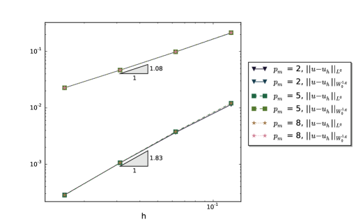
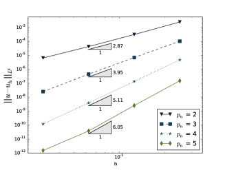
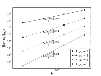
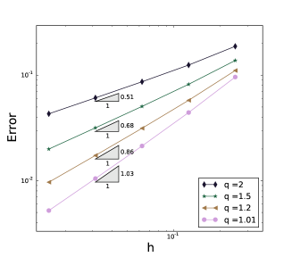
We start with investigating the convergence of the proposed method with weak boundary conditions on the inflow boundary in the space , i.e., formulation (4.3) with from (4.6), and the norm (4.4) with and . To this end, we first consider the convergence of the method for Example 5.2 with . We consider a uniform mesh with element size . The space consists of piecewise polynomials of degree , while space consists of piecewise polynomials of degree on the same mesh with . Figure 1 shows that for the error is essentially independent of the choice of and hence there is no benefit to enriching the space of the residual beyond . Figure 2 shows that we obtain the expected optimal convergence rates for different polynomial degrees under uniform -refinement.
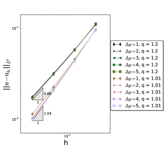
Next, we consider the same example with the same finite element spaces for . Figure 3 (left) shows that again both for and the error does not improve as is increased beyond ; for , however, we can observe that the error is larger for . Note that we did not observe this in the diffusive regime. The plot on the right shows that in the convection-dominated regime we obtain a convergence rate of approximately as tends to zero; this is consistent with the approximation error bound of the piecewise linear interpolant of a jump discontinuity.
5.2 Convection-Diffusion in 1D
In this section we consider different choices for , and and show how this affects the approximation to the solution of Example 5.1. To this end, in Section 5.2.1, we investigate how the choice of , and the boundary conditions in affect the approximation . In Section 5.2.2 we consider one specific choice for the test norm and show that the oscillations vanish entirely as . Next, in Section 5.2.3, we investigate the choice of the finite element space more closely. We have seen that increasing has no significant effect on the convergence rates; however, we will see that this does indeed affect certain qualitative properties of the solution. Finally, we demonstrate that the method is robust in in Section 5.2.4
5.2.1 Comparing the Choices for the Test Norm and the Boundary Conditions
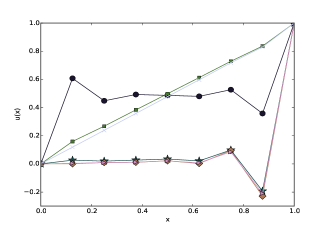
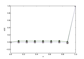
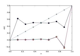
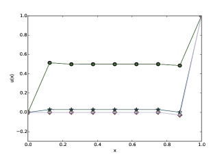
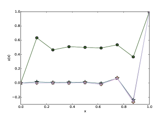
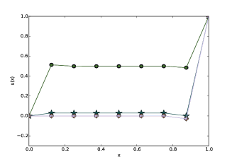
We start by comparing different versions of the non-linear Petrov-Galerkin method. In order to ensure that the space is sufficiently large we use piecewise polynomials of degree as the basis, while consists of piecewise linear polynomials. We split the interval uniformly into elements. We consider three different choices for the weighting function as mentioned in Section 4.1, namely , and . We combine this with two different choices of boundary conditions on , i.e., zero Dirichlet boundary conditions on the whole boundary and weak boundary conditions on the inflow boundary as described in Section 4.2. This creates six test cases; we first consider these six test cases for with and . Secondly, we consider all six test cases with , and The solution for each of the cases is shown in Figure 4.
We can see in Figures 4(a), 4(c) and 4(e) that for and Dirichlet boundary conditions on the whole boundary for , the approximation only resembles the analytical solution if . Introducing weak boundary conditions on on the inflow boundary resolves this issue for but the approximation with only shows improvement if . These observations are the same for and . This indicates that we can circumvent constructing a non-constant function – which can be challenging for complicated geometries – by introducing weak boundary conditions on on the inflow boundary. These observations are consistent with the results for a very similar problem studied in [19]. Furthermore, note that and most closely resembles the method introduced in [7]. In [7] it is demonstrated for a different (two-dimensional) example that the approximation for can be very inaccurate.
If we now consider , cf., Figures 4(b), 4(d) and 4(f), we observe a different behaviour of the approximation. If , the approximations are all very similar and much closer to the analytical solution with close to no undershoots; we will investigate the phenomenon of vanishing undershoots more closely both in one dimension and two dimensions later on. If , the approximation with Dirichlet boundary conditions on the whole boundary and or again leads to a very poor approximation to the analytical solution. This again points to robustness issues that for are only visible for much smaller than for . An interesting observation is that for , the combination of weak inflow boundary conditions on and is not distinguishable from other choices of for whereas, for it is significantly different. The improvement of the approximation as for and resembles the results presented in [7].
In conclusion, choosing the boundary conditions as described in Section 4.2 allows us to avoid constructing a non-constant weighting function . Close to , the results are very similar for and , whereas close to , clearly yields a significantly better approximation of the solution.
The choice of does not seem to have a big impact on the approximation except in the case and , where choosing improves the approximation compared to . If , then both for and , the dominant term in the norm on is essentially since and are the same up to a constant in one dimension. If , then implies that is endowed with the -norm , whereas for the -term is the dominant term in the norm on due to the -weighting of the gradient. Since yields a better approximation in this case, this suggests that for it is favourable to choose a stronger norm on that is either dominated by the norm of the gradient or the streamline term .

5.2.2 Vanishing oscillations as
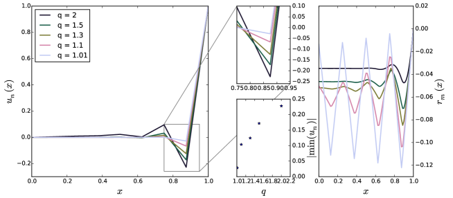
The examples in Figure 4 already illustrate that the undershoot in the approximate solution nearly vanishes for . We will now investigate in more detail how the undershoot depends on if we choose , , and impose weak inflow boundary conditions on . To this end, we choose a large space with polynomial degree and piecewise linear polynomials for . We split the interval into elements and compute the approximate solutions for several choices of . Figure 5 shows on the left and on the right. A close-up of the undershoot and a plot vs. is shown in the centre of the figure. We can see that the undershoot decreases monotonically as approaches . In contrast to this, we can see that the oscillations in the residual increase as which suggests that a large space may be necessary. This is the next aspect of the method we will investigate.
5.2.3 The Choice of the Space
In [17], it has been shown that the inexact method is well-posed if a Fortin projector, cf., (3.11) exists. It is easy to see that is a necessary condition. Finding a sufficient condition or in other words finding a compatible pair is highly non-trivial. In [40], certain special cases for the convection-reaction equation are considered. The observations in Section 5.1 suggest that for , the Fortin condition is typically satisfied. We now investigate how the choice of affects the undershoot for close to . To this end, we consider two different strategies of enlarging : global -enrichment and uniform -refinement. We again consider , , and impose weak inflow boundary conditions on .
p-enrichment: In terms of implementation, the simplest choice for the space such that is a finite element space over the same grid with the polynomial degree increased globally by some integer . Figure 6 shows how the overshoot reduces as we increase . The difference in for varying is barely visible even though we have used a finer mesh for plotting in order to capture the behaviour of the higher modes and yet it has a significant effect on the approximation .
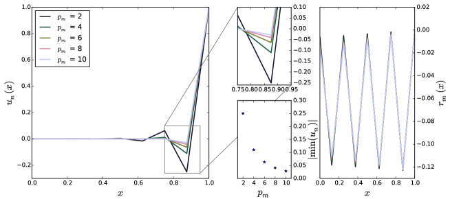
h-refinement: This time both and consist of piecewise linear polynomials. To ensure that , we choose a refinement of the underlying mesh of the space to construct the space . This is the only numerical experiment in this article that cannot be implemented in FEniCS; instead, e.g., the C++ library Hermes2D [41] can be used. Figure 7 shows how the overshoot reduces as we refine the mesh for ;
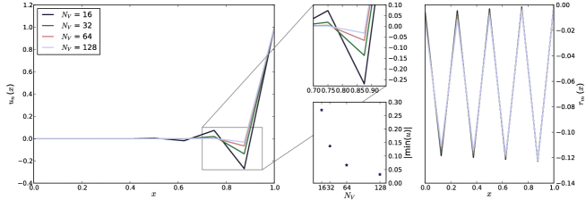
the difference in is again barely visible despite the significant effect on the approximation .
5.2.4 Robustness in
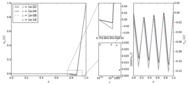
As a final experiment in one dimension, we study how affects the undershoot in the approximation. We continue with the same setting as in the previous section, but keep fixed as the space of piecewise polynomials of degree on the same mesh as used for and vary instead. Figure 8 shows that, although the undershoot is not the same for all leading to an under resolved layer, the undershoot seems to be approximately the same for all for some . This can be traced back to the inflow boundary conditions on — which are scaled with — if we look at on the right in Figure 8. The method therefore seems to be robust in .
5.3 Vanishing Oscillations in Two Dimensions
In this section we explore whether the under- and overshoots in the approximation still vanish as if we apply the method to two-dimensional problems. To this end, we consider the Examples 5.2, 5.3 and 5.4 on different meshes for . We consider , and impose weak boundary conditions on as described in Section 4.2. In one case we will also consider to compare the approximations for both choices of . We will see that the overshoots disappear on certain meshes, but remain present on others. We will furthermore demonstrate that the approximation qualitatively behaves like the -best approximation of the analytical solution and thus we can apply the observations in [5] to (a) predict on which meshes the overshoot will disappear as and (b) design meshes that have this property in specific situations.
5.3.1 The Eriksson-Johnson Model Problem
We consider the Eriksson-Johnson Model Problem (Example 5.2) on the four different meshes depicted in Figure 9. Note that these are the same meshes that are investigated in [5].
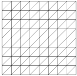
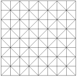
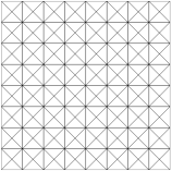
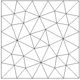
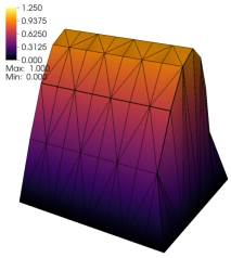
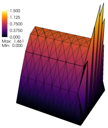
First, we compare the approximations on Mesh 2 and Mesh 3 for and with the interpolant of the analytical solution in . Figure 10 shows the approximations on Mesh 2; for we clearly observe overshoots near the boundary layer (center) compared to the interpolant of the analytical solution (left). On the other hand, for we can see that the approximation approaches the interpolant of the analytical solution. Figure 11 shows the approximations on Mesh 3; in this case we can see that the overshoot is nearly the same for and . From [5] we note that this is the qualitative behaviour that the -best approximation exhibits.
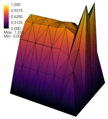
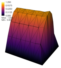
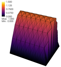
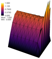
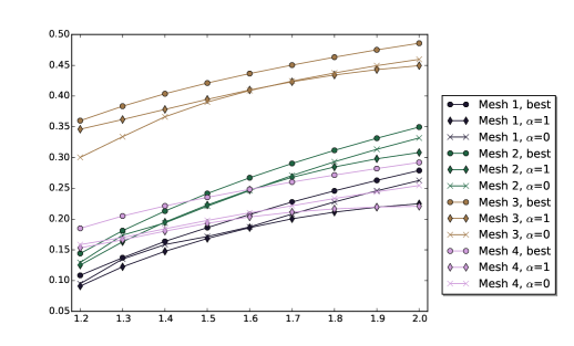
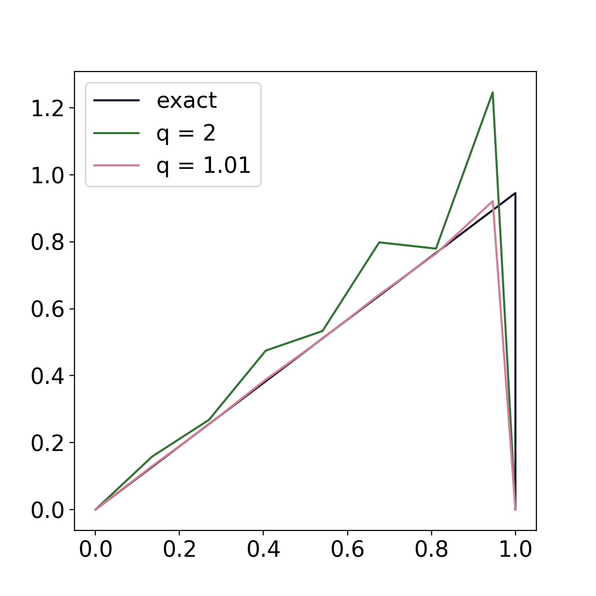
With this in mind, we have numerically computed the -best approximation of the analytical solution for several choices of and have also computed the finite element approximations with and both, and , with weak boundary conditions imposed on on the inflow boundary for the same values of . Figure 12 shows the maximal error between the interpolant of the analytical solution and the approximation for the -best approximation and the error between the interpolant and the numerical approximations for and . We can clearly see that the overshoot observed for our proposed scheme is very similar to the overshoot in the -best approximation. Therefore, understanding for which meshes discontinuities/layers are captured as sharply as the grid allows by the -best approximation can serve as an indicator regarding whether the over- and undershoots dissappear as . This is the subject of [5], where the -best approximation of discontinuous functions is analysed in detail in certain cases.
5.3.2 Boundary Layer in a Corner of the Domain
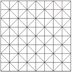
In this section we consider Example 5.3 with . We will see that on Mesh 2 in this case the overshoot does not disappear as for our method. This is due to the layer not only appearing along an edge of the unit square but also near the corner . With this in mind, we suggest an alternative mesh that is only a slight modification of Mesh 2 for which the overshoot disappears. Figure 13 shows the two versions of Mesh 2 that we have used and the corresponding approximations for and along the line through the interior nodes closest to the boundary . We can see that on Mesh 2, the overshoot near the corner does not disappear as , whereas it does reduce significantly away from the corner. For the modified version of Mesh 2, the overshoot disappears everywhere as .
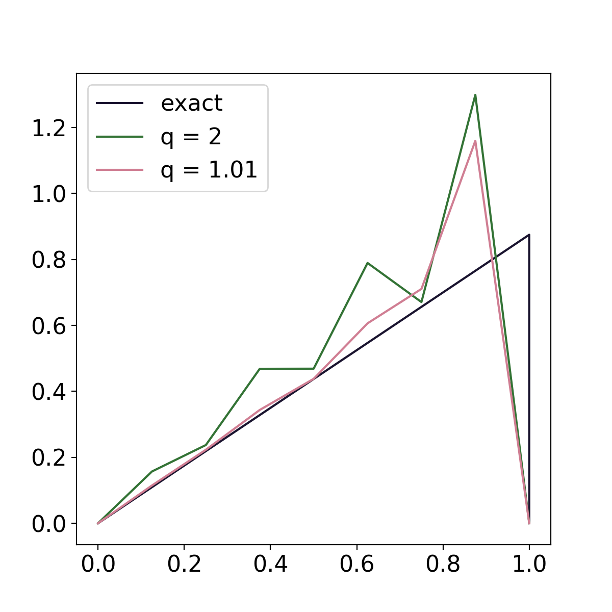
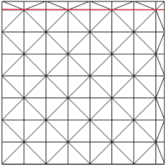
To understand the improvement when using this modified mesh, we focus on the interior node closest to the corner . Figure 14 shows all elements connected to this node. The elements with either a node or an edge on the boundary are marked in green; the elements separated from the boundary are blue. From [5] we can infer that the -best approximation does not exhibit overshoots if the volume of the green area is smaller or equal to the volume of the blue area. This is obviously violated on Mesh 2 with the green area being three times as large as the blue area. The modified version of the mesh is designed to satisfy this condition by changing the mesh as indicated in Figure 14.
5.3.3 Example with an Interior Layer
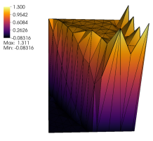
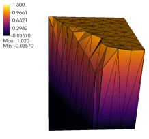
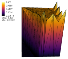
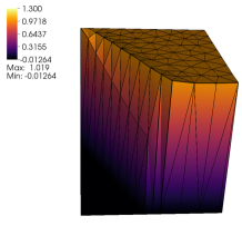
In this section we consider Example 5.4 and demonstrate that a mesh can be constructed such that the over- and undershoots both near the boundary layer and the interior layer can be eliminated as . To this end, Figure 15 shows the approximation to Example 5.4 for and on two different meshes. The first mesh is designed such that the overshoot at the boundary layer disappears as ; this is already clearly visible for . Along the interior layer, the overshoot also reduces significantly, but some over- and undershoots are still present for . The second mesh is additionally designed to align with the interior layer in such a way that we can expect the over- and undershoots to disappear as . We can see, that this mesh even nearly eliminates the overshoot along the interior layer for and for all over- and undershoots along both layers have essentially vanished.
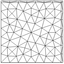
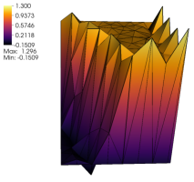
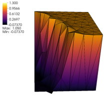
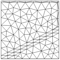
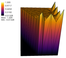
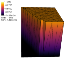
Figure 16 shows the approximations for and if is not perfectly aligned with the mesh, i.e., and . The difference between these two choices for is that in the latter case the layer is still contained in between the two lines parallel to the line , whereas in the former case it is not. In both cases, we clearly observe overshoots along the interior layer for which are reduced for . Both, for and the overshoot reduces slowly the closer is to . For and the overshoot is barely visible in Figure 16, but comparing the maximum and minimum values of the approximations reveals that the over- and undershoots are similar to the case in magnitude.
6 Conclusions and Future Directions
In this article, we generalized the framework employed for DPG methods to more general Banach spaces. This framework in principle allows us to choose the norm in which the solution is approximated, provided a suitable well-posed variational formulation with robust constants and a test-norm that is computable is given. Another challenge in designing such a method is that a Fortin-condition must be satisfied for the discrete spaces and . The recent work [42] describes a double adaptivity approach for the DPG method to circumvent this challenge in the context of DPG methods. Due to the close relationship between DPG methods and our approach this has potential to be generalized to the Banach space framework.
Furthermore, we have demonstrated how to design a finite element method for the convection-diffusion-reaction problem that in the convection-dominated case yields solutions that qualitatively behave like the -best approximation of the analytical solution. This means that on meshes where the -best approximation does not contain any over- and undershoots, these can also be avoided by taking in our proposed method. Indeed, the final two examples presented in this article demonstrate that it is possible to adjust meshes to specific situations in order to eliminate over- and undershoots.
An important implication of the connection to the -best approximation is that we can use the insights from [5] to design suitable meshes. Note that even in one dimension the over- and undershoots will not disappear for certain non-uniform meshes. Roughly speaking, meshes where the elements near the discontinuity or layer present in the analytical solution are smaller than at a distance from those features are more favourable. Additionally, it is desirable that all interior nodes that are closest to such a feature are aligned roughly in parallel with the feature; for further details, we refer to [5]. This is similar to the observations used to design the modified version of the mesh in the final two examples. This suggests that if the mesh is refined in a suitable way near the layer, we can eliminate over- and undershoots. This observation could be used to design a mesh refinement strategy that modifies the mesh in such a way that the -best approximation of the layer or discontinuity does not contain any over- or undershoots. Note, however, that even though we modified the mesh in the final example in a way that resembles refinement towards the boundary layer, the boundary layer clearly remains under resolved even on the modified mesh. It is therefore not necessary to fully resolve the layer to eliminate the oscillations in this case.
Another challenge of our proposed method is computational feasibility. Possible strategies to addressing this include reducing the degrees of freedom by choosing the test space adaptively, introducing broken test spaces , similar to DPG methods, to allow for more effective parallelization, and developing a more efficient non-linear solver. Despite the challenges outlined above, the numerical results for our proposed method show great potential for the application to non-linear problems whose analytical solutions contain sharp layers or discontinuities. It is well-known that higher-order monotonicity preserving methods can be expected to be non-linear; thus, the non-linear nature of our approach by no means diminishes its potential.
Acknowledgements
The authors would like to thank Gabriel Barrenechea, Jesse Chan, Leszek Demkowicz, Jay Gopalakrishnan, Ignacio Muga and Martin Stynes for fruitful discussions on the topic of this article.
References
- [1] J. W. Gibbs, Fourier’s series, Nature 59 (1539) (1899) 606.
- [2] H. Wilbraham, On a certain periodic function, Cambridge and Dublin Math. J 3 (198) (1848) 1848.
- [3] F. Richards, A Gibbs phenomenon for spline functions, Journal of approximation theory 66 (3) (1991) 334–351.
- [4] E. B. Saff, S. Tashev, Gibbs phenomenon for best approximation by polygonal lines, East J. Approx. 5 (2) (1999) 235–251.
- [5] P. Houston, S. Roggendorf, K. G. van der Zee, Gibbs Phenomenon for -Best Approximation of Discontinuities in Finite Element Spaces – Some Examples (Unpublished Result).
- [6] E. Moskona, P. Petrushev, E. Saff, The gibbs phenomenon for best L1-trigonometric polynomial approximation, Constructive Approximation 11 (3) (1995) 391–416.
- [7] J.-L. Guermond, A finite element technique for solving first-order PDEs in , SIAM J. Numer. Anal. 42 (2) (2004) 714–737.
- [8] J. E. Lavery, Nonoscillatory solution of the steady-state inviscid Burgers’ equation by mathematical programming, J. Comput. Phys. 79 (2) (1988) 436–448.
- [9] J. E. Lavery, Solution of steady-state one-dimensional conservation laws by mathematical programming, SIAM J. Numer. Anal. 26 (5) (1989) 1081–1089.
- [10] J. E. Lavery, Solution of steady-state, two-dimensional conservation laws by mathematical programming, SIAM J. Numer. Anal. 28 (1) (1991) 141–155.
- [11] B.-N. Jiang, Non-oscillatory and non-diffusive solution of convection problems by the iteratively reweighted least-squares finite element method, Journal of computational physics 105 (1) (1993) 108–121.
- [12] B.-N. Jiang, The least-squares finite element method: theory and applications in computational fluid dynamics and electromagnetics, Springer Science & Business Media, 1998.
- [13] J.-L. Guermond, B. Popov, Linear advection with ill-posed boundary conditions via -minimization, Int. J. Numer. Anal. Model. 4 (1) (2007) 39–47.
- [14] J.-L. Guermond, F. Marpeau, B. Popov, A fast algorithm for solving first-order PDEs by -minimization, Commun. Math. Sci. 6 (1) (2008) 199–216.
- [15] J.-L. Guermond, B. Popov, -approximation of stationary Hamilton-Jacobi equations, SIAM J. Numer. Anal. 47 (1) (2008/09) 339–362.
- [16] J.-L. Guermond, B. Popov, An optimal -minimization algorithm for stationary Hamilton-Jacobi equations, Commun. Math. Sci. 7 (1) (2009) 211–238.
- [17] I. Muga, K. G. van der Zee, Discretization of Linear Problems in Banach Spaces: Residual Minimization, Nonlinear Petrov-Galerkin, and Monotone Mixed Methods, arXiv preprint arXiv:1511.04400v2 (2017).
- [18] L. F. Demkowicz, J. Gopalakrishnan, An overview of the discontinuous Petrov Galerkin method, in: Recent developments in discontinuous Galerkin finite element methods for partial differential equations, Vol. 157 of IMA Vol. Math. Appl., Springer, Cham, 2014, pp. 149–180.
- [19] J. Chan, J. A. Evans, W. Qiu, A dual Petrov-Galerkin finite element method for the convection-diffusion equation, Comput. Math. Appl. 68 (11) (2014).
- [20] D. Broersen, R. Stevenson, A robust Petrov-Galerkin discretisation of convection-diffusion equations, Comput. Math. Appl. 68 (11) (2014) 1605–1618.
- [21] D. Broersen, R. P. Stevenson, A Petrov-Galerkin discretization with optimal test space of a mild-weak formulation of convection-diffusion equations in mixed form, IMA J. Numer. Anal. 35 (1) (2015) 39–73.
- [22] J. Chan, N. Heuer, T. Bui-Thanh, L. Demkowicz, A robust DPG method for convection-dominated diffusion problems II: adjoint boundary conditions and mesh-dependent test norms, Comput. Math. Appl. 67 (4) (2014) 771–795.
- [23] A. Cohen, W. Dahmen, G. Welper, Adaptivity and variational stabilization for convection-diffusion equations, ESAIM Math. Model. Numer. Anal. 46 (5) (2012) 1247–1273.
- [24] L. Demkowicz, N. Heuer, Robust DPG method for convection-dominated diffusion problems, SIAM J. Numer. Anal. 51 (5) (2013) 2514–2537.
- [25] M. S. Alnæs, J. Blechta, J. Hake, A. Johansson, B. Kehlet, A. Logg, C. Richardson, J. Ring, M. E. Rognes, G. N. Wells, The FEniCS project version 1.5, Archive of Numerical Software 3 (100) (2015).
- [26] A. Logg, K.-A. Mardal, G. N. Wells, et al., Automated Solution of Differential Equations by the Finite Element Method, Springer, 2012.
- [27] I. Muga, K. G. van der Zee, Discretization of Linear Problems in Banach Spaces: Residual Minimization, Nonlinear Petrov-Galerkin, and Monotone Mixed Methods, arXiv preprint arXiv:1511.04400v1 (2015).
- [28] P. Houston, I. Muga, S. Roggendorf, K. G. van der Zee, The Convection-Diffusion-Reaction Equation in Non-Hilbert Sobolev Spaces: A Direct Proof of the Inf-Sup Condition and Stability of Galerkin’s Method, Comput. Methods Appl. Math. 19 (3) (2019) 503–522.
- [29] H. Brezis, Functional analysis, Sobolev spaces and partial differential equations, Universitext, Springer, New York, 2011.
- [30] K. Deimling, Nonlinear functional analysis, Springer-Verlag, Berlin, 1985.
- [31] E. Zeidler, Nonlinear functional analysis and its applications. III, Springer-Verlag, New York, 1985, variational methods and optimization, Translated from the German by Leo F. Boron.
- [32] I. Cioranescu, Geometry of Banach spaces, duality mappings and nonlinear problems, Vol. 62 of Mathematics and its Applications, Kluwer Academic Publishers Group, Dordrecht, 1990.
- [33] C. Chidume, Geometric properties of Banach spaces and nonlinear iterations, Vol. 1965 of Lecture Notes in Mathematics, Springer-Verlag London, Ltd., London, 2009.
- [34] L. Demkowicz, J. Gopalakrishnan, Discontinuous Petrov-Galerkin (DPG) method, ICES Report (15–20) (2015).
- [35] L. Demkowicz, J. Gopalakrishnan, A class of discontinuous Petrov-Galerkin methods. II. Optimal test functions, Numer. Methods Partial Differential Equations 27 (1) (2011) 70–105.
- [36] I. Stakgold, M. J. Holst, Green’s functions and boundary value problems, Vol. 99, John Wiley & Sons, 2011.
- [37] J. Zitelli, I. Muga, L. Demkowicz, J. Gopalakrishnan, D. Pardo, V. M. Calo, A class of discontinuous Petrov-Galerkin methods. Part IV: the optimal test norm and time-harmonic wave propagation in 1D, J. Comput. Phys. 230 (7) (2011) 2406–2432.
- [38] J. Gopalakrishnan, W. Qiu, An analysis of the practical DPG method, Mathematics of Computation 83 (286) (2014) 537–552.
- [39] J. Gopalakrishnan, Five lectures on DPG methods, arXiv:1306.0557 (2013).
- [40] I. Muga, M. J. W. Tyler, K. G. van der Zee, The Discrete-Dual Minimal-Residual Method (DDMRes) for Weak Advection-Reaction Problems in Banach Spaces, Comput. Methods Appl. Math. 19 (3) (2019) 557–579.
- [41] P. Solin, L. Korous, P. Kus, Hermes2D, a C++ library for rapid development of adaptive -FEM and -DG solvers, J. Comput. Appl. Math. 270 (2014) 152–165.
- [42] L. Demkowicz, T. Fürer, N. Heuer, X. Tian, The double adaptivity paradigm (how to circumvent the discrete inf-sup conditions of babuška and brezzi), ICES Report (19–07) (2019).