Application of renormalized RPA to polarized Fermi gases

Abstract

We consider a spin imbalanced Fermi gas at zero temperature in the normal phase on the BCS side of the BCS-BEC crossover and around unitarity. We compute the critical polarization for pairing, the correlated occupation numbers and the contact in an extension of particle-particle RPA (also called non self-consistent T-matrix approach or ladder approximation). The so-called renormalized RPA consists in computing the T matrix with self-consistently determined occupation numbers. The occupation numbers are determined either by keeping the self-energy only to first order or by resumming the Dyson equation. In this way, the result for the critical polarization, strongly overestimated in standard RPA, is clearly improved. We also discuss some problems of this approach.

I Introduction

Cold atoms have allowed for the first realization of the crossover from superfluidity of Cooper pairs as described by the Bardeen-Cooper-Schrieffer (BCS) theory to Bose-Einstein condensation (BEC) of dimers. This is possible because the scattering length $a$, i.e., the interaction strength, can be changed thanks to the Feshbach resonance. At zero temperature, a Fermi gas with two spin states $\sigma=\uparrow,\downarrow$ of equal masses and populations is superfluid at any interaction strength. This is not the case for a polarized gas, in which pairing disappears beyond some critical polarization $P_{c}$ whose value depends on the interaction strength. In the polarized case, other forms of pairing may exist such as the Fulde-Ferrell-Larkin-Ovchinnikov (FFLO) phase Fulde and Ferrell (1964); Larkin and Ovchinnikov (1964) characterized by an oscillating order parameter corresponding to pairs with a non-zero total momentum. So far, in experiments on polarized Fermi gases performed on resonance ($a\to\infty$, the so-called unitary limit) Partridge et al. (2006); Shin et al. (2006, 2008a) and in the BCS-BEC crossover Shin et al. (2008b); Olsen et al. (2015), the FFLO phase was not seen, but a phase separation into a paired and an unpaired state was found. In fact, the FFLO phase may be difficult to see in a harmonic trap and the use of flat traps may clarify this question in the future. The problem of pairing in asymmetric systems has also been studied, e.g., in the case of proton-neutron pairing in asymmetric nuclear matter Stein et al. (2014) and in the context of QCD with color superconductivity in the case of quark matter which also involves particles of different masses Alford et al. (2008).

Many theoretical studies have already addressed the problem of pairing in polarized Fermi gases, for reviews see Radzihovsky and Sheehy (2010); Chevy and Mora (2010); Gubbels and Stoof (2013). One problem of polarized systems is that the standard Nozières and Schmitt-Rink (NSR) Nozières and Schmitt-Rink (1985) approach, which describes the BCS-BEC crossover at finite temperature, fails in the polarized case Liu and Hu (2006); Parish et al. (2007). Different variants of the NSR approach were proposed to solve this problem Kashimura et al. (2012); Chen et al. (2007); He et al. (2007); Pantel et al. (2014). All these approaches have in common to be based on the ladder approximation for the in-medium T matrix and to include the self-energy in a somewhat more self-consistent way than it is done in the NSR theory.

In this paper, we consider only the case of zero temperature and the normal phase. This implies that the polarization of the gas must exceed the critical polarization $P_{c}$ below which superfluidity sets in. The ladder approximation becomes then equivalent to what is known in nuclear physics as the particle-particle Random-Phase Approximation (pp-RPA) which was applied to polarized Fermi gases in Urban and Schuck (2014). The pp-RPA gives satisfactory results on the BCS side for not too strong interaction, but at unitarity it overestimates strongly the critical polarization. Within this formalism, the onset of superfluidity appears as an instability, but it is not possible to describe the superfluid phase. Maybe one could generalize the formalism to the superfluid phase using Gor’kov Green’s functions, similarly to what was done in the unpolarized case at finite temperature, e.g., in Pieri et al. (2004), but this is beyond the scope of the present study.

From a general perspective, the RPA describes correlations in the medium, e.g., the correlation energy or correlated occupation numbers, starting from an uncorrelated ground state. In this sense, the RPA is not fully consistent. Different extensions of RPA were developed to take into account these correlations in a more consistent way. One of them is the self-consistent RPA (SCRPA) Dukelsky et al. (1998); Schäfer and Schuck (1999); Hirsch et al. (2002), which is based on the correlated RPA ground state. In practice, however, the SCRPA is very difficult to implement except in simple toy models. An approximation to the SCRPA is the renormalized RPA (r-RPA) Catara et al. (1996); Delion et al. (2005), which instead of using the correlated ground state uses only the correlated occupation numbers in the calculation. The inclusion of the correlated occupation numbers can be expected to solve, at least partially, the problem of the critical polarization in the polarized Fermi gas at zero temperature.

Our article is organized as follows. In Sec. II, we recall briefly the pp-RPA formalism and describe the basic idea of the self-consistent processing of the occupation numbers. We use two different methods to obtain the occupation numbers, one based on the Dyson equation truncated at first order that we call RPA(1st), and the other using the full Dyson equation that we call RPA($\infty$). We will discuss the results obtained for the occupation numbers and the contact. In Sec. III, we present the calculation of the critical polarization, first in the case of RPA and then in the case of the r-RPA. Finally, we conclude in Sec. IV.

II Self-consistent occupation numbers

II.1 Recapitulation of pp-RPA at zero temperature

Let’s start by recalling the pp-RPA for a zero-temperature polarized fermion gas. At zero temperature, it is common to fix the densities of up and down populations, denoted $\rho_{\uparrow}$ and $\rho_{\downarrow}$, unlike at finite temperature where one usually fixes the chemical potentials. The polarization $P$ of the gas is then defined as

$$P=\dfrac{\rho_{\uparrow}-\rho_{\downarrow}}{\rho_{\uparrow}+\rho_{\downarrow}}\,,$$ (1)

assuming $\rho_{\uparrow}>\rho_{\downarrow}$ as convention. Since the formalism breaks down at the superfluid phase transition (see Sec. III), we limit ourselves to sufficiently strong polarizations where the system remains normal fluid even at zero temperature.

The pp-RPA is based on the formalism of the in-medium T matrix which is written as the sum of ladder diagrams that we can see in Fig. 1 (a).

Figure 1: Representation in terms of Feynman diagrams of (a) the vertex function $\Gamma$, (b) the self-energy $\Sigma$, and the occupation numbers $n^{\sigma}$ calculated with (c) the truncated Dyson equation [RPA(1st)] and (d) the full Dyson equation [RPA($\infty$)]. Inserting self-consistent occupation numbers into the two-particle propagator $J$ within the r-RPA corresponds roughly to an approximate way of dressing the thick blue lines in diagram (a), but there is no one-to-one correspondence in terms of diagrams.

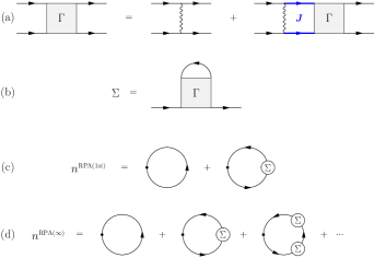
In the case of cold atoms, it is appropriate to take a contact interaction with coupling constant $g$. The vertex function $\Gamma$ is written as

$$\Gamma(\operatorname{\textbf{\text{k}}},\,\omega)=\dfrac{1}{1/g-J(\operatorname{\textbf{\text{k}}},\,\omega)}\,,$$ (2)

with $J(\operatorname{\textbf{\text{k}}},\,\omega)=J_{hh}(\operatorname{\textbf{\text{k}}},\,\omega)+J_{pp}(\operatorname{\textbf{\text{k}}},\,\omega)$, including both particle-particle (pp) and hole-hole (hh) propagation. The function $J$ needs to be regularized Perali et al. (2002) which gives the following expressions:

$$g=\dfrac{4\pi a}{m}\,,$$ (3)

$$J_{hh}(\operatorname{\textbf{\text{k}}},\omega)=-\int\dfrac{\mathrm{d}^{3}\mathbf{p}}{(2\pi)^{3}}\,\dfrac{n^{\uparrow}(|\frac{\operatorname{\textbf{\text{k}}}}{2}+\operatorname{\mathbf{p}}|)\,n^{\downarrow}(|\frac{\operatorname{\textbf{\text{k}}}}{2}-\operatorname{\mathbf{p}}|)}{\omega-\varepsilon_{\frac{\operatorname{\textbf{\text{k}}}}{2}+\operatorname{\mathbf{p}}}-\varepsilon_{\frac{\operatorname{\textbf{\text{k}}}}{2}-\operatorname{\mathbf{p}}}-\operatorname{i}\eta}\,,$$ (4)

$$J_{pp}(\operatorname{\textbf{\text{k}}},\omega)=\int\dfrac{\mathrm{d}^{3}\mathbf{p}}{(2\pi)^{3}}\left(\dfrac{\bar{n}^{\uparrow}(|\frac{\operatorname{\textbf{\text{k}}}}{2}+\operatorname{\mathbf{p}}|)\,\bar{n}^{\downarrow}(|\frac{\operatorname{\textbf{\text{k}}}}{2}-\operatorname{\mathbf{p}}|)}{\omega-\varepsilon_{\frac{\operatorname{\textbf{\text{k}}}}{2}+\operatorname{\mathbf{p}}}-\varepsilon_{\frac{\operatorname{\textbf{\text{k}}}}{2}-\operatorname{\mathbf{p}}}+\operatorname{i}\eta}+\dfrac{m}{p^{2}}\right)\,,$$ (5)

where $\varepsilon_{\operatorname{\textbf{\text{k}}}}=k^{2}/(2m)$, $n^{\sigma}$ are the occupation numbers of spin $\sigma$, and $\bar{n}^{\sigma}=1-n^{\sigma}$. In the case of standard RPA, the expression of $n^{\sigma}$ is $n^{\sigma}(k)=\theta(k_{\text{\tiny{F}}}^{\sigma}-k)$.

To calculate the correlated occupation numbers $n^{\sigma}$ in standard RPA, one uses the Dyson equation truncated at first order [Fig. 1 (c)], i.e.,

$$G^{\sigma}=G_{0}^{\sigma}+G_{0}^{\sigma}\Sigma^{\sigma}G_{0}^{\sigma}\,,$$ (6)

where $G^{\sigma}$ is the dressed Green’s function, $G_{0}^{\sigma}$ the bare Green’s function and $\Sigma^{\sigma}$ the self-energy represented in Fig. 1 (b), which has the form

$$\Sigma^{\sigma}(\operatorname{\textbf{\text{k}}},\,\omega)=-\operatorname{i}\int\!\dfrac{\mathrm{d}^{3}\mathbf{p}}{(2\pi)^{3}}\int\!\dfrac{\mathrm{d}\omega^{\prime}}{2\pi}G_{0}^{\bar{\sigma}}(\operatorname{\mathbf{p}},\,\omega^{\prime})\,\Gamma(\operatorname{\textbf{\text{k}}}+\operatorname{\mathbf{p}},\,\omega+\omega^{\prime})\,,$$ (7)

where $\bar{\sigma}$ denotes the spin opposite to $\sigma$. This is the same approximation that is used at finite temperature in the NSR theory Nozières and Schmitt-Rink (1985). The general expression for the occupation numbers reads Fetter and Walecka (1975)

$$n^{\sigma}(k)=-\operatorname{i}\int\dfrac{\mathrm{d}\omega}{2\pi}\,\operatorname{e}^{\operatorname{i}\omega\eta}G^{\sigma}(\operatorname{\textbf{\text{k}}},\omega)\,.$$ (8)

The resulting expressions for the occupation numbers of the holes and particles are respectively Urban and Schuck (2014)

$$n^{\sigma}(k<k_{\text{\tiny{F}}}^{\sigma})=1+\int\!\dfrac{\mathrm{d}^{3}\mathbf{p}}{(2\pi)^{3}}\int_{\Omega_{\text{\tiny{F}}}}^{+\infty}\dfrac{\mathrm{d}\omega}{\pi}\,\dfrac{\theta(k_{\text{\tiny{F}}}^{\bar{\sigma}}-|\operatorname{\mathbf{p}}-\operatorname{\textbf{\text{k}}}|)}{(\omega-\varepsilon_{\operatorname{\textbf{\text{k}}}}-\varepsilon_{\operatorname{\mathbf{p}}-\operatorname{\textbf{\text{k}}}})^{2}}\\ \times\operatorname{\mathcal{I}m}\Gamma(\operatorname{\mathbf{p}},\,\omega)\,,$$ (9)

$$n^{\sigma}(k>k_{\text{\tiny{F}}}^{\sigma})=-\int\dfrac{\mathrm{d}^{3}\mathbf{p}}{(2\pi)^{3}}\,\int_{-\infty}^{\Omega_{\text{\tiny{F}}}}\dfrac{\mathrm{d}\omega}{\pi}\,\dfrac{\theta(|\operatorname{\mathbf{p}}-\operatorname{\textbf{\text{k}}}|-k_{\text{\tiny{F}}}^{\bar{\sigma}})}{(\omega-\varepsilon_{\operatorname{\textbf{\text{k}}}}-\varepsilon_{\mathbf{p}-\operatorname{\textbf{\text{k}}}})^{2}}\\ \times\operatorname{\mathcal{I}m}\Gamma(\operatorname{\mathbf{p}},\,\omega)\,,$$ (10)

where $\Omega_{\text{\tiny{F}}}=(k_{\text{\tiny{F}}}^{\uparrow\,2}+k_{\text{\tiny{F}}}^{\downarrow\,2})/(2m)$ is the energy separating the two-particle and two-hole continua. The occupation numbers that we obtain can be decomposed into a continuous part $n_{c}$ and a step of height $Z^{\sigma}=\lim\limits_{\varepsilon\rightarrow 0}n^{\sigma}(k_{\text{\tiny{F}}}^{\sigma}-\varepsilon)-n^{\sigma}(k_{\text{\tiny{F}}}^{\sigma}+\varepsilon)$, i.e.,

$$n^{\sigma}(k)=Z^{\sigma}\,\theta(k_{\text{\tiny{F}}}^{\sigma}-k)+n_{c}^{\sigma}(k)\,.$$ (11)

On the one hand, the procedure of keeping in Eq. (6) only the first order in the self-energy makes it possible to satisfy the Luttinger theorem, i.e., that the correlations do not modify the densities of the gas. On the other hand, it leads to a pathology when the interaction becomes too strong, the height of the step $Z$ becoming negative (and occupation numbers can become negative, too) Urban and Schuck (2014).

II.2 Renormalized pp-RPA

The idea of renormalized RPA (r-RPA) is to reuse the pp-RPA formalism presented in the preceding subsection but in which the occupation numbers in Eqs. (4) and (5) are no longer Heaviside functions but the correlated occupation numbers writted in Eq. (11). This approximation can be justified using the equation-of-motion method for the two-particle Green’s function, see, e.g., Dukelsky et al. (1998).

In some sense, this prescription can be viewed as an approximation to the two-particle Green’s function $J$ one would obtain by dressing the single-particle propagators appearing in the ladder diagrams in Fig. 1 (a). However, there are important differences. For instance, in the limit $P\to 1$, the r-RPA reduces to the RPA because the up and down occupation numbers tend to $\theta(k_{\text{\tiny{F}}}^{\uparrow}-k)$ and $0$, respectively, while the dressed propagator of the down particle (polaron) would remain non-trivial even in this limit.

By including the correlations ($Z^{\sigma}<1$) in the calculation of the two-particle propagator $J$, the logarithmic singularity of $\operatorname{\mathcal{R}e}J$, responsible for the instability of the normal phase Fetter and Walecka (1975), will be reduced. This can be seen in Fig. 2, where we show $J(\operatorname{\textbf{\text{k}}},\omega)$ for small non-vanishing $\operatorname{\textbf{\text{k}}}$ for better visibility.

Figure 2: Imaginary and real part of $J$ as function of $\omega$ for $k=0.01\,k_{\text{\tiny{F}}}^{\uparrow}$ and $k_{\text{\tiny{F}}}^{\downarrow}=k_{\text{\tiny{F}}}^{\uparrow}/2$. The blue solid lines represent $J$ with uncorrelated occupation numbers and the red dash-dotted lines are obtained with self-consistent occupation numbers for $a\,k_{\text{\tiny{F}}}^{\uparrow}=-2$.

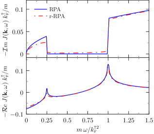
This softening of the singularity will allow the normal phase to remain stable at lower polarization.

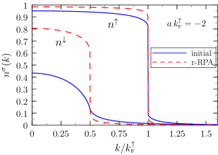
With this formalism, the results of the pp-RPA can be considered as the first iteration of the self-consistent calculation. To carry out the iteration, the correlated occupation numbers are calculated according to Eqs. (9) and (10) and are reinjected into the functions $J$, Eqs. (4) and (5). This procedure is repeated until convergence is reached. One important thing to notice is that the converged result is independent of the initial occupation numbers. The comparison between the RPA and r-RPA occupation numbers is shown in Fig. 3 for different values of the interaction strength.

Figure 3: Up and down occupation numbers for the polarization $k_{\text{\tiny{F}}}^{\downarrow}=k_{\text{\tiny{F}}}^{\uparrow}/2$ ($P=0.778$) for the RPA (blue solid line) and the r-RPA (at convergence, red dashed line). (a) $a\,k_{\text{\tiny{F}}}^{\uparrow}=-2$, (b) $a\,k_{\text{\tiny{F}}}^{\uparrow}=-3$. The inset shows a zoom on the unphysical negative step ($Z^{\downarrow}<0$) of the down occupation numbers.

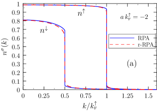
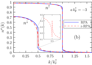
For weak interactions, i.e., $|a\,k_{\text{\tiny{F}}}^{\uparrow}|<1$, the r-RPA provides virtually no correction to the RPA. In contrast, for stronger interactions, ​​the r-RPA reduces the value of $Z$ more strongly than the RPA calculation. Therefore the self-consistent treatment does not cure the pathology of RPA that the value of $Z$ becomes negative for interactions that are too strong; on the contrary, the negative step appears already for weaker interactions (for instance, in Fig. 3(b), the step of $n^{\downarrow}(k)$ is negative in r-RPA as can be seen in the zoom).

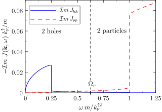
Let us note that it follows from the spectral representation of the two-particle Green function $J$ (see chapter 15.2 of Blaizot and Ripka (1986)) that in principle the two-hole continuum of $\operatorname{\mathcal{I}m}J_{hh}$ should be restricted to energies below $\Omega_{\text{\tiny{F}}}$ and the two-particle continuum of $\operatorname{\mathcal{I}m}J_{pp}$ to energies above $\Omega_{\text{\tiny{F}}}$, as it is the case in standard pp-RPA. In the self-consistent treatment, i.e., by including the correlations in the calculation of $J$, we see that the two-particle continuum $\operatorname{\mathcal{I}m}J_{pp}$ extends into the two-hole continuum and vice versa as shown in Fig. 4. This is a general problem of the r-RPA approach.

Figure 4: Imaginary part of $J$ as function of $\omega$ for $\operatorname{\textbf{\text{k}}}=\boldsymbol{0}$ and $k_{\text{\tiny{F}}}^{\downarrow}=k_{\text{\tiny{F}}}^{\uparrow}/2$. The blue line is the imaginary part of $J$ for holes and the red dashed line for particles. As can be seen, each curve extends into the energy zone of the other.

II.3 Contact

A very interesting property of the occupation numbers is the asymptotic behavior of the momentum distribution tails. In the case of a contact interaction, the asymptotic behavior ($k\gg k_{\text{\tiny{F}}}^{\sigma}$) follows the power law $n^{\sigma}(k)\sim C/k^{4}$. The coefficient

$$C=\lim_{k\to\infty}k^{4}n^{\uparrow}(k)=\lim_{k\to\infty}k^{4}n^{\downarrow}(k)$$ (12)

is independent of the spin and, in the notation of Tan Tan (2008a, b), it is called contact. This relationship has been restated in a field theory context in Ref. Braaten and Platter (2008). The value of the contact $C$ is related to different thermodynamic properties of the Fermi gas Tan (2008b, c). For instance, it determines the dependence of the energy density $E/V$ on the interaction strength as Tan (2008b)

$$\frac{d(E/V)}{d(-1/a)}=\frac{C}{4\pi m}\,.$$ (13)

Figure 5 shows the dependence of the contact $C$ on the interaction and polarization parameters for the RPA and the r-RPA.

Figure 5: Contact $C$ (a) as a function of the interaction for an asymmetry of $k_{\text{\tiny{F}}}^{\downarrow}=k_{\text{\tiny{F}}}^{\uparrow}/2$; (b) as a function of the polarization for interactions of $a\,k_{\text{\tiny{F}}}^{\uparrow}=-1$ and $a\,k_{\text{\tiny{F}}}^{\uparrow}=-2$. The blue solid lines are the RPA results and the red dashed lines are for the r-RPA. The black dashed-dotted line represents the perturbative expression for the contact in the weakly interacting limit.

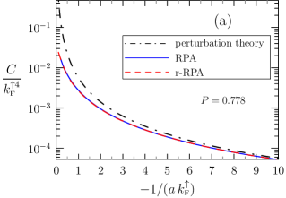
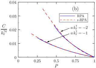
Note that the value of the contact is almost identical within the RPA and the r-RPA, we do not know if the small difference between these curves is only due to the numerical precision or not. In the limit of weak interaction (large $-1/(a\,k_{\text{\tiny{F}}}^{\uparrow}))$, the contact approaches the perturbative result $C=16\pi^{2}\,a^{2}\,\rho^{\uparrow}\rho^{\downarrow}$ Calvanese Strinati et al. (2018), as can be seen in Fig. 5.

II.4 Occupation numbers calculated with the full Dyson equation

The problem of the negative step that appears in the occupation numbers calculated with the standard RPA when the interaction becomes too strong is not improved by the self-consistent treatment. One way to cure this pathology is to use the complete Dyson equation instead of the truncated version (6) presented in Sec. II.1, i.e., to dress the Green function as

$$G=\dfrac{1}{1/G_{0}-\Sigma}\,.$$ (14)

In terms of diagrams, the occupation numbers calculated with the complete Dyson equation are represented in Fig. 1 (d).

When we consider the complete equation (14) to calculate the occupation numbers, the self-energy $\Sigma$, Eq. (7), must be explicitly calculated, which is not the case when using the first-order truncated Dyson equation (6) as done before. The expressions for the imaginary part of the self-energy $\Sigma=\Sigma_{hh}+\Sigma_{pp}$ are given by Urban and Schuck (2014)

$$\operatorname{\mathcal{I}m}\Sigma_{hh}^{\sigma}(\operatorname{\textbf{\text{k}}},\,\omega)=-\int_{p>k_{\text{\tiny{F}}}^{\bar{\sigma}}}\dfrac{\mathrm{d}^{3}\mathbf{p}}{(2\pi)^{3}}\,\theta(\Omega_{\text{\tiny{F}}}-\omega-\varepsilon_{\operatorname{\mathbf{p}}})\\ \times\operatorname{\mathcal{I}m}\Gamma(\operatorname{\textbf{\text{k}}}+\operatorname{\mathbf{p}},\,\omega+\varepsilon_{\operatorname{\mathbf{p}}})\,,$$ (15)

$$\operatorname{\mathcal{I}m}\Sigma_{pp}^{\sigma}(\operatorname{\textbf{\text{k}}},\,\omega)=\int_{p<k_{\text{\tiny{F}}}^{\bar{\sigma}}}\dfrac{\mathrm{d}^{3}\mathbf{p}}{(2\pi)^{3}}\,\theta(\omega+\varepsilon_{\operatorname{\mathbf{p}}}-\Omega_{\text{\tiny{F}}})\\ \times\operatorname{\mathcal{I}m}\Gamma(\operatorname{\textbf{\text{k}}}+\operatorname{\mathbf{p}},\,\omega+\varepsilon_{\operatorname{\mathbf{p}}})$$ (16)

and the corresponding real parts are calculated with a dispersion relation. Then we calculate the spectral function

$$A^{\sigma}(\operatorname{\textbf{\text{k}}},\,\omega)=-\operatorname{\mathcal{I}m}\dfrac{1}{\omega-\epsilon_{\operatorname{\textbf{\text{k}}}}-\Sigma^{\sigma}(\operatorname{\textbf{\text{k}}},\,\omega-U^{\sigma})}\,.$$ (17)

We have introduced the quantity $U^{\sigma}=\operatorname{\mathcal{R}e}\Sigma^{\sigma}(k_{\text{\tiny{F}}},\,\varepsilon_{\text{\tiny{F}}})$ to take into account the shift of the Fermi energy caused by the real part of $\Sigma$. A useful property of the spectral function is

$$\int_{\varepsilon_{\text{\tiny{F}}}+U^{\sigma}}^{+\infty}\dfrac{\mathrm{d}\omega}{\pi}\,A^{\sigma}(\operatorname{\textbf{\text{k}}},\,\omega)-\int_{-\infty}^{\varepsilon_{\text{\tiny{F}}}+U^{\sigma}}\dfrac{\mathrm{d}\omega}{\pi}\,A^{\sigma}(\operatorname{\textbf{\text{k}}},\,\omega)=1\,.$$ (18)

The occupation numbers are obtained from

$$n^{\sigma}(k)=\pm\int_{-\infty}^{\varepsilon_{\text{\tiny{F}}}+U^{\sigma}}\dfrac{\mathrm{d}\omega}{\pi}\,A^{\sigma}(\operatorname{\textbf{\text{k}}},\,\omega)\,,$$ (19)

with $+$ for holes and $-$ for particles. To avoid having to integrate the peak present in the spectral function when calculating the occupation numbers of the holes, we use Eq. (18) that normalizes the spectral function and integrate over the complementary interval where there is no peak. Finally this leads to the formulas

$$n^{\sigma}(k<k_{\text{\tiny{F}}}^{\sigma})=1-\int_{\varepsilon_{\text{\tiny{F}}}+U^{\sigma}}^{+\infty}\dfrac{\mathrm{d}\omega}{\pi}\,A^{\sigma}(\operatorname{\textbf{\text{k}}},\,\omega)\,,$$ (20)

$$n^{\sigma}(k>k_{\text{\tiny{F}}}^{\sigma})=-\int_{-\infty}^{\varepsilon_{\text{\tiny{F}}}+U^{\sigma}}\dfrac{\mathrm{d}\omega}{\pi}\,A^{\sigma}(\operatorname{\textbf{\text{k}}},\,\omega)\,.$$ (21)

By comparing the results of this method, denoted RPA($\infty$), and those of the standard RPA (RPA(1st)), we see in Fig. 6 that the occupation numbers within the RPA($\infty$) are less modified than those within RPA(1st). In particular, the negative step disappears even at the strongest interactions. Roughly speaking, since $Z_{1\text{st}}\simeq 1+\mathrm{d}\Sigma/\mathrm{d}\omega$ and $Z_{\infty}\simeq 1/(1-\mathrm{d}\Sigma/\mathrm{d}\omega)$ the step heights of the two methods are related by $Z_{1\text{st}}\simeq 2-1/Z_{\infty}$. For weak interactions, both methods give similar results.

Figure 6: The solid blue lines represent the occupation numbers calculated with RPA(1st), i.e., the truncated Dyson equation (6) and the dashed red lines represent the occupation numbers calculated with RPA($\infty$), i.e., the complete Dyson equation (14). The polarization is fixed at $k_{\text{\tiny{F}}}^{\downarrow}=k_{\text{\tiny{F}}}^{\uparrow}/2$, interaction strength is $a\,k_{\text{\tiny{F}}}^{\uparrow}=-4$. The $Z^{\downarrow}$ calculated with RPA($\infty$) decreases much less than with the RPA(1st).

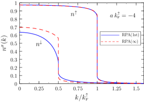
To set up self-consistency, we adopt the same approach as in Sec. II.2. Figure 7 shows the difference of the occupation numbers calculated with the r-RPA(1st) and r-RPA($\infty$).

Figure 7: Same as Fig. 6 but using self-consistent occupation numbers (r-RPA). $Z^{\downarrow}$ calculated with r-RPA($\infty$) is positive whereas the one calculated with r-RPA(1st) is negative.

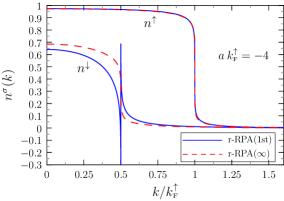
Again, in the occupation numbers calculated with the full Dyson equation, the problem of the negative step (and even negative occupation numbers) present in the r-RPA(1st) has disappeared.

However there is a price to pay. If we define $\rho_{\sigma}^{\text{\tiny{L}}}=k_{\text{\tiny{F}}}^{\sigma\,3}/(6\pi^{2})$, the Luttinger theorem Luttinger (1960) states that the density $\rho_{\sigma}$ calculated as the integral of the correlated occupation numbers satisfies the relation $\rho_{\sigma}=\rho_{\sigma}^{\text{\tiny{L}}}$. As shown in Urban and Schuck (2014) this is exactly fulfilled within RPA(1st), but it is no longer true if the occupation numbers are calculated with the full Dyson equation (RPA($\infty$)). More quantitatively, we define the relative error $\Delta_{\text{\tiny{rel}}}^{\sigma}=|\rho_{\sigma}^{\text{\tiny{L}}}-\rho_{\sigma}|/\rho_{\sigma}$. Table 1 shows the violation of the Luttinger theorem for one specific example ($a\,k_{\text{\tiny{F}}}^{\uparrow}=-2.5$, $k_{\text{\tiny{F}}}^{\downarrow}=k_{\text{\tiny{F}}}^{\uparrow}/2$).

Table 1: Relative error $\Delta_{\text{\tiny{rel}}}^{\sigma}$ (violation of the Luttinger theorem) for different calculations with $a\,k_{\text{\tiny{F}}}^{\uparrow}=-2.5$ and $k_{\text{\tiny{F}}}^{\downarrow}=k_{\text{\tiny{F}}}^{\uparrow}/2$

	RPA(1st)	r-RPA(1st)	RPA($\infty$)	r-RPA($\infty$)
$\Delta_{\text{\tiny{rel}}}^{\uparrow}$	$0$	$0.053\,\%$	$0.073\,\%$	$0.013\,\%$
$\Delta_{\text{\tiny{rel}}}^{\downarrow}$	$0$	$0.45\,\%$	$2.9\,\%$	$2.1\,\%$

We see that only the RPA(1st) satisfies the Luttinger theorem exactly. However, the r-RPA(1st) violates the Luttinger theorem only very slightly and the error observed can be due to the accumulation of numerical errors. The RPA($\infty$), on the contrary, clearly violates the Luttinger theorem and therefore the r-RPA($\infty$), too. At stronger interactions, the violation within RPA($\infty$) and r-RPA($\infty$) can be much worse, e.g., near the critical polarization at the unitary limit (see Sec. III.3).

III Critical polarization

III.1 FFLO transition

The Thouless criterion Thouless (1960) states that the superfluid transition occurs when a pole appears in the T matrix at $\omega=\Omega_{\text{\tiny{F}}}$, i.e., $1/g-J(\operatorname{\textbf{\text{k}}},\omega=\Omega_{\text{\tiny{F}}})=0$. As long as the condition $1/g-J(\operatorname{\textbf{\text{k}}},\Omega_{\text{\tiny{F}}})<0$ is fulfilled for all $\operatorname{\textbf{\text{k}}}$, we are in the normal phase as shown in Fig. 8 as the blue dashed curve.

Figure 8: Typical behavior of $1/g-J(\operatorname{\textbf{\text{k}}},\Omega_{\text{\tiny{F}}})$ (computed within RPA for $a\,k_{\text{\tiny{F}}}^{\uparrow}=-1.913$) as function of $k$ for five polarizations $P$. At the three highest polarizations associated with lower three (blue, black and purple) curves, the system is in the normal phase. The green solid line is at the critical polarization $P_{c}$ where the function vanishes for a value of $k$ which corresponds to $k_{\text{\tiny{FFLO}}}$. The red dash-dotted line is obtained for the value of the polarization which gives the pole at $\operatorname{\textbf{\text{k}}}=\boldsymbol{0}$ (BCS superfluidity), but it lies already in the FFLO superfluid region. For the definitions of $P_{\text{\tiny{L}}}$ and $a_{\text{\tiny{M}}}$, see text.

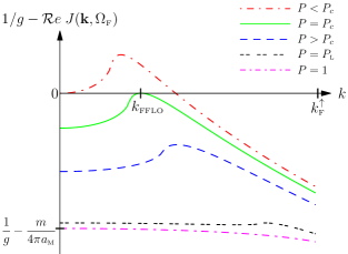
In the case of a non-polarized gas at finite temperature, approaching $T_{c}$ from above, the instability of the normal phase sets in first at $\operatorname{\textbf{\text{k}}}=\boldsymbol{0}$. However, in the case of a polarized gas, the difference between the Fermi levels favors the creation of pairs with non-zero total momentum, resulting in the emergence of a new type of superfluidity called FFLO phase Fulde and Ferrell (1964); Larkin and Ovchinnikov (1964). Now we look for the appearance of the pole when approaching $P_{c}$ from above. Considering $1/g-J(\operatorname{\textbf{\text{k}}},\Omega_{\text{\tiny{F}}})$ as function of $k$ for different values of $P$, as shown in Fig. 8, we notice that the pole at $\operatorname{\textbf{\text{k}}}\neq\boldsymbol{0}$ appears at a higher polarization than the one at $\operatorname{\textbf{\text{k}}}=\boldsymbol{0}$. The value of $k$ at which the pole appears first, coming from strong polarization, is denoted $k_{\text{\tiny{FFLO}}}$:

$$1/g-\operatorname{\mathcal{R}e}J(\mathbf{k}_{\text{\tiny{FFLO}}},\Omega_{\text{\tiny{F}}})=\max_{k}\left(1/g-\operatorname{\mathcal{R}e}J(\operatorname{\textbf{\text{k}}},\Omega_{\text{\tiny{F}}})\right)\,.$$ (22)

To determine the critical polarization, we must therefore determine the value of $P$ such that

$$1/g-\operatorname{\mathcal{R}e}J(\mathbf{k}_{\text{\tiny{FFLO}}},\Omega_{\text{\tiny{F}}})=0\,.$$ (23)

At the critical polarization, there is an instability of the system towards a formation of pairs with momentum $k_{\text{\tiny{FFLO}}}$. Therefore $k_{\text{\tiny{FFLO}}}$ corresponds more or less to the wave vector of the order-parameter oscillations in the FFLO phase. However, our theory does not tell us whether the paired phase that will be formed corresponds to a Fulde-Ferrel (FF) state with just one wave vector Larkin and Ovchinnikov (1964), a Larkin-Ovchinnikov (LO) state with spatial modulations of the order parameter but without a varying phase Fulde and Ferrell (1964), or even more complicated states with a crystal-like structure.

The qualitative picture described above and illustrated in Fig. 8 remains the same in a large range of interaction strengths $1/(ak_{\text{\tiny{F}}})$. Increasing $1/(ak_{\text{\tiny{F}}})$, i.e., $1/g$, simply shifts the curves upwards and thereby increases the critical polarization, which in turn leads to a higher value of $k_{\text{\tiny{FFLO}}}$. The dependence of $k_{\text{\tiny{FFLO}}}$ computed within RPA as a function of the ratio $k_{\text{\tiny{F}}}^{\downarrow}/k_{\text{\tiny{F}}}^{\uparrow}$ (which is directly related to $P$, small values of $k_{\text{\tiny{F}}}^{\downarrow}/k_{\text{\tiny{F}}}^{\uparrow}$ corresponding to large $P$ and vice versa) is displayed in Fig. 9 as the solid blue line.

Figure 9: Value of $k_{\text{\tiny{FFLO}}}$ as a function of $k_{\text{\tiny{F}}}^{\downarrow}/k_{\text{\tiny{F}}}^{\uparrow}$ within RPA (solid blue line) and within r-RPA($\infty$) (dashed red line). In RPA, it is independent of the strength of the interaction. For the r-RPA($\infty$), we have used $a\,k_{\text{\tiny{F}}}^{\uparrow}$ for each $k_{\text{\tiny{F}}}^{\downarrow}/k_{\text{\tiny{F}}}^{\uparrow}$ such that $P=P_{c}$. The FFLO phase disappears for $k_{\text{\tiny{F}}}^{\downarrow}/k_{\text{\tiny{F}}}^{\uparrow}<0.224$ in the RPA, and for $k_{\text{\tiny{F}}}^{\downarrow}/k_{\text{\tiny{F}}}^{\uparrow}<0.435$ in the r-RPA($\infty$).

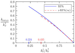
At some positive value of $1/g$, corresponding to a strong critical polarization, the picture changes. As it can be seen from the double-dashed black curve in Fig. 8, at some strong polarization denoted $P_{\text{\tiny{L}}}$, the local maximum at $k=k_{\text{\tiny{FFLO}}}$ has become so flat that its value coincides with another local maximum that has built up at $k=0$. Hence, at $P=P_{\text{\tiny{L}}}$, the global maximum of $1/g-J$ changes from the one at $k\neq 0$ to the one at $k=0$, and as a consequence, $k_{\text{\tiny{FFLO}}}$ jumps from a finite value to zero, as can be seen in Fig. 9. This corresponds to the Lifshitz point L in the schematic phase diagram of Son and Stephanov (2006).

III.2 Implementation of self-consistency

As explained in the preceding subsection, for fixed values of $k_{\text{\tiny{F}}}^{\uparrow}$ and $a$, the method to find the critical polarization is to determine the zero of $1/g-J(\operatorname{\textbf{\text{k}}}_{\text{\tiny{FFLO}}},\Omega_{\text{\tiny{F}}})$ as a function of $P$, i.e., in practice as a function of $k_{\text{\tiny{F}}}^{\downarrow}$. This curve is shown in Fig. 10.

Figure 10: Schematic behavior of the maximum value of the function $1/g-\operatorname{\mathcal{R}e}J(\operatorname{\textbf{\text{k}}},\Omega_{\text{\tiny{F}}})$ depending on $k_{\text{\tiny{F}}}^{\downarrow}$ for fixed $k_{\text{\tiny{F}}}^{\uparrow}$. The blue solid line is obtained from the RPA and the red dashed line from the r-RPA. As can be seen, the critical polarization obtained from r-RPA is in the superfluid phase of the RPA.

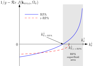
The value of $k_{\text{\tiny{F}}}^{\downarrow}$ corresponding to $P_{c}$ will be denoted $k_{\text{\tiny{F,c}}}^{\downarrow}$. For values of $k_{\text{\tiny{F}}}^{\downarrow}$ lower than $k_{\text{\tiny{F,c}}}^{\downarrow}$, we are in the normal phase, otherwise we are in the superfluid phase which cannot be described with our theory.

However, it is impossible to compute this curve for the r-RPA up to the corresponding $k_{\text{\tiny{F,c}}}^{\downarrow}$ (for given $a$ and $k_{\text{\tiny{F}}}^{\uparrow}$) if one initializes the self-consistent iteration with the uncorrelated occupation numbers (step functions). The reason becomes clear from Fig. 10: with increasing correlations, $P_{c}$ becomes smaller, i.e., $k_{\text{\tiny{F,c}}}^{\downarrow}$ becomes larger. Therefore, $k_{\text{\tiny{F,c}}}^{\downarrow}$ for r-RPA lies in the superfluid area of RPA and already the first iteration step cannot be performed. To avoid going through the superfluid zone, we need to find initial conditions that maximize the correlations and at the same time $k_{\text{\tiny F,c}}^{\downarrow}$ so that it decreases with each iteration. Fortunately the result is independent of the initial occupation numbers. The occupation numbers for the initialization are constructed from those calculated with the RPA by artificially increasing as much as possible the correlated part $\delta n^{\sigma}(k)=n^{\sigma}(k)-\theta(k_{\text{\tiny{F}}}^{\sigma}-k)$ such that $Z^{\downarrow}=0$ (cf. Fig. 11).

Figure 11: Up and down occupation numbers for the polarization $k_{\text{\tiny{F}}}^{\downarrow}=k_{\text{\tiny{F}}}^{\uparrow}/2$ ($P=0.778$) and $a\,k_{\text{\tiny{F}}}^{\uparrow}=-2$. Solid blue lines represent the occupation numbers used for the initialization of the self-consistent iteration. Dashed red lines represent the converged occupation numbers within the r-RPA(1st) calculation.

We then use the procedure described in the preceding section to find the $k_{\text{\tiny{FFLO}}}$. In the r-RPA($\infty$), we observe a more and more important deviation from the RPA as the polarization increases as can be seen by comparing the solid blue and the dashed red lines in Fig. 9. Also the critical value of $k_{\text{\tiny{F}}}^{\downarrow}$ changes (where $k_{\text{\tiny{FFLO}}}$ disappears). In RPA, we find this point at $(k_{\text{\tiny{F}}}^{\downarrow}/k_{\text{\tiny{F}}}^{\uparrow})_{\text{\tiny{L}}}=0.224$ and slightly on the BEC side close to unitarity at $1/(a_{\text{\tiny{L}}}k_{\text{\tiny{F}}}^{\uparrow})\simeq 0.210$, in agreement with the disappearence of the FFLO phase in mean-field theory, see Fig. 6(a) of Calvanese Strinati et al. (2018). In r-RPA($\infty$), we find $(k_{\text{\tiny{F}}}^{\downarrow}/k_{\text{\tiny{F}}}^{\uparrow})_{\text{\tiny{L}}}=0.435$ at $1/(a_{\text{\tiny{L}}}k_{\text{\tiny{F}}}^{\uparrow})\simeq 0.131$ which is closer to the unitarity compared to the RPA result. It is due to the fact that the maximum that gives the $k_{\text{\tiny{FFLO}}}$ becomes flatter with the self-consistency. Therefore, it drops more quickly below the global maximum at $k=0$ and the FFLO phase is lost.

III.3 Phase diagram

Following the procedure discussed in the preceding subsections, we are only able to detect the instability of the normal phase corresponding to a second-order phase transition to the superfluid phase. However, if there is a first-order phase transition from the normal to the superfluid phase with a coexistence region extending to a higher polarization than our critical polarization $P_{c}$, we are not able to see it, because this would require to compute the energy of the superfluid phase. Keeping this word of caution in mind, we show in Fig. 12 the phase diagram giving the critical polarization as a function of the interaction strength.

Figure 12: Critical polarization from the Thouless criterion as function of $-1/(a\,k_{\text{\tiny{F}}}^{\uparrow})$. Thick lines correspond to $P_{c}$ calculated with the occupation numbers and thin lines to $P_{c}^{\text{\tiny{L}}}$ that one would obtain if the Luttinger theorem was satisfied. The blue solid lines represent the RPA calculation. The red lines are for r-RPA(1st), in the range where they are dotted it gives a negative step ($Z<0$). The green dashed lines are for r-RPA($\infty$). The black cross is the theoretical prediction extracted from Fig. 1 of Ref. Bulgac and Forbes (2008). We also show experimental results for the limit of the coexistence region corresponding to a first-order phase transition towards an unpolarized superfluid phase; the data are from Refs. Shin et al. (2008a, b) (Shin et al.) and Olsen et al. (2015) (Olsen et al.).

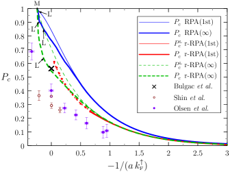
Notice that on the BEC side of the crossover, beyond some interaction $-1/(a_{\text{\tiny{M}}}k_{\text{\tiny{F}}}^{\uparrow})<0$, the polarized normal phase (except at $P=1$ where the system is non-interacting) does not exist any more. This point, denoted M, corresponds to the polaron-to-molecule transition discussed in Refs. Prokof’ev and Svistunov (2008); Punk et al. (2009) where few down particles added to a fully polarized system of up particles do not form a normal fluid Fermi sea of polarons any more, but a BEC of molecules with total momentum $k=0$. In the present framework, this transition happens when the lowest curve shown in Fig. 8, corresponding to $P=1$, is shifted upwards to the horizontal axis, i.e., at

$$\frac{1}{a_{\text{\tiny{M}}}k_{\text{\tiny{F}}}^{\uparrow}}=\frac{4\pi}{mk_{\text{\tiny{F}}}^{\uparrow}}J(0,\varepsilon_{\text{\tiny{F}}};k_{\text{\tiny{F}}}^{\downarrow}=0)=\frac{2}{\pi}-\frac{1}{\sqrt{2}\pi}\ln\frac{\sqrt{2}+1}{\sqrt{2}-1}\\ \simeq 0.24\,.$$ (24)

This value has to be compared with the exact one, $1/(a_{\text{\tiny{M}}}k_{\text{\tiny{F}}}^{\uparrow})\simeq 0.9$ Prokof’ev and Svistunov (2008). The origin of this discrepancy is that the ladder approximation includes only 2-particle (2p) but no 3-particle-1-hole (3p1h) and more complicated states Punk et al. (2009). Since at $P_{c}=1$ no down particles are present any more, the self-consistency does not have any effect and all our curves, whether they are calculated with RPA or r-RPA, end in the same point M.

Next to the point M, we have the transition towards the $k=0$ superfluid phase. Only to the right of the Lifshitz point L mentioned in Sec. III.1, visible as kink in the curves pointed by the black arrows in Fig. 12, the transition is of the FFLO type.

We see that, as expected, the critical polarization in r-RPA is always lower than in RPA. Notice that the r-RPA(1st) (red lines) breaks down at interactions stronger than $1/(a\,\smash{k_{\text{\tiny{F}}}^{\uparrow}})\simeq-0.675$ where a negative step appears in the occupation numbers. Nevertheless, it is still possible to reach convergence in some range and these results are shown as red dotted lines in Fig. 12. In contrast to the r-RPA(1st), the r-RPA($\infty$), shown as the green dashed lines, allows us to describe the whole range of interactions up to the point M, since a negative step does not appear. At weak interaction, the computation with r-RPA($\infty$) gives the same result as r-RPA(1st) which is obvious since the occupation numbers are practically the same in this case.

The critical polarization within RPA is actually the same as within mean field including the possibility of the FFLO phase but no phase separation Pao and Yip (2009) (see also Fig. 6(a) of Calvanese Strinati et al. (2018)). In particular, in the unitary limit, the RPA predicts $P_{c}=0.834$. This is clearly higher than the critical polarization $P_{c}=0.562$ obtained from an energy-density functional (ASLDA) fitted to Quantum-Monte-Carlo (QMC) results Bulgac and Forbes (2008), marked by the cross in Fig. 12. Thus the r-RPA($\infty$) result of $P_{c}=0.543$ (thick dashed line) would be a significant improvement compared to the RPA. However this low $P_{c}$ is to some extent a consequence of the violation of the Luttinger theorem. In fact, if one computes $P_{c}$ under the assumption that the Luttinger theorem is satisfied, i.e., $P_{c}^{\text{\tiny{L}}}=(k_{\text{\tiny{F}}}^{\uparrow 3}-k_{\text{\tiny{F}}}^{\downarrow 3})/(k_{\text{\tiny{F}}}^{\uparrow 3}+k_{\text{\tiny{F}}}^{\downarrow 3})$, one obtains only a weaker reduction from $0.834$ to $0.709$ (thin dashed line).

Since in RPA(1st) the Luttinger theorem is exactly fulfilled, we have $P_{c}^{\text{\tiny{L}}}(\text{RPA(1st)})=P_{c}(\text{RPA(1st)})$ (thin blue line). Since the RPA($\infty$) uses the same uncorrelated occupation numbers as the RPA(1st), it is clear that also $P_{c}^{\text{\tiny{L}}}(\text{RPA($\infty$)})=P_{c}(\text{RPA(1st)})$. The reduction of $P_{c}(\text{RPA($\infty$)})$ (thick blue line) near unitarity is therefore only due to the violation of the Luttinger theorem. The violation of the Luttinger theorem in RPA($\infty$) and r-RPA($\infty$) gets stronger and stronger as we approach the unitary limit. It becomes visible in the region of interaction and polarization parameters where the RPA(1st) and r-RPA(1st) give a negative step. On the contrary, for the r-RPA(1st), we have $P_{c}(\text{r-RPA(1st)})\simeq P_{c}^{\text{\tiny{L}}}(\text{r-RPA(1st)})$ for all values of interaction, therefore we tend to suspect that the Luttinger theorem is fulfilled for the r-RPA(1st) and that the small discrepancy comes from the accumulation of numerical errors. Finally, treating the RPA with the Dyson equation avoids occupation numbers with negative steps but there are still unphysical features.

Finally, let us say a few words about the phase separation observed in Shin et al. (2008a, b); Olsen et al. (2015). These experiments indicate that at the polarizations shown by the circles in Fig. 12, there is a first-order phase transition towards an unpolarized superfluid, in good agreement with QMC results which did not include the possibility of FFLO-type phases Pilati and Giorgini (2008). The experimental critical polarization for phase separation is much lower than the one obtained in mean field Pao and Yip (2009) and leaves some room for a possible continuous (second order) transition towards the FFLO phase before phase separation happens, which corresponds qualitatively to the scenario suggested in Bulgac and Forbes (2008) for the case of unitarity.

IV Conclusions

We have implemented a self-consistent calculation of the occupation numbers in the formalism of the r-RPA. This is an approximation to the so-called self-consistent RPA (by RPA we mean the RPA in the particle-particle channel, pp-RPA). On the one hand, in the context of polarized Fermi gases, the r-RPA is interesting because it reduces the critical polarization at $T=0$ that is strongly overestimated with RPA. The r-RPA is therefore an improvement in the description of this system. On the other hand, the formalism does not cure certain pathologies specific to the RPA. One of the problems of standard RPA [RPA(1st)] is that in the strongly coupled regime the quasiparticle $Z$ factor at the Fermi surface (i.e., the height of the step in the occupation numbers) becomes negative. A way to cure this pathology is to consider the complete Dyson equation [RPA($\infty$)] instead of the truncated one which is used in RPA(1st) (and also in the NSR approach at finite temperature). This method does not conserve the number of particles (Luttinger theorem) but it gives at least physical occupation numbers for arbitrary strength of interaction.

Other self-consistent calculations exist to treat in-medium correlations in cold atoms. These numerically demanding methods are based on the self-consistent Green’s functions also called Luttinger-Ward formalism at finite temperature. These methods were applied to study the finite temperature BCS-BEC crossover, in particular the phase diagram of non-polarized Haussmann (1994); Haussmann et al. (2007) and polarized Frank et al. (2018) gases. In Pieri and Strinati (2017), it was shown that within the Luttinger-Ward formalism, the Luttinger theorem is exactly fulfilled with the full Dyson equation.

The r-RPA method allows us to see the evolution of occupation numbers by including correlations in the ground state. An interesting aspect is that the tails of the occupation numbers, whose information is contained in the contact term, remains almost unchanged with the inclusion of self-consistency.

We discussed the transition to the superfluid phase as an instability in the T matrix (Thouless criterion). Except at very strong polarizations (beyond the Lifshitz point), the transition is predicted to be of the FFLO type and our r-RPA result for the corresponding critical polarization in the unitary limit is close to the one of LABEL:Bulgac2008.

Although the FFLO phase has attracted a lot of attention (also in the context of imbalanced gases with two components of different masses Forbes et al. (2005)), its existence is still an open question. In particular, there is a competition between phase separation (as seen in experiments) and the formation of the FFLO phase Bulgac and Forbes (2008); Bedaque et al. (2003); Liu and Wilczek (2003); Son and Stephanov (2006). With the present theory, which is limited to the normal phase, we cannot address the question of phase separation because it requires the calculation of the energy in the superfluid phase. The FFLO phase and phase separation can perhaps be reconciled by interpreting the FFLO phase (to be precise, the LO phase) as a periodic “micro-phase separation” Radzihovsky and Sheehy (2010). Furthermore, as it was pointed out, e.g., in Radzihovsky and Sheehy (2010), the harmonic potential of the trap makes it difficult to see the FFLO phase in experiments. Hopefully, future experiments with flat traps as they are being built will clarify this question.

References

- Fulde and Ferrell (1964) P. Fulde and R. A. Ferrell, Physical Review 135, A550 (1964).
- Larkin and Ovchinnikov (1964) A. I. Larkin and Y. N. Ovchinnikov, Zh. Eksp. Teor. Fiz. 47, 1136 (1964).
- Partridge et al. (2006) G. B. Partridge, W. Li, R. I. Kamar, Y.-a. Liao, and R. G. Hulet, Nature 311, 503 (2006).
- Shin et al. (2006) Y.-i. Shin, M. W. Zwierlein, C. H. Schunck, A. Schirotzek, and W. Ketterle, Phys. Rev. Lett. 97, 049901 (2006).
- Shin et al. (2008a) Y.-i. Shin, C. H. Schunck, A. Schirotzek, and W. Ketterle, Nature 451, 689 (2008a).
- Shin et al. (2008b) Y.-i. Shin, A. Schirotzek, C. H. Schunck, and W. Ketterle, Phys. Rev. Lett. 101, 070404 (2008b).
- Olsen et al. (2015) B. A. Olsen, M. C. Revelle, J. A. Fry, D. E. Sheehy, and R. G. Hulet, Phys. Rev. A 92, 063616 (2015).
- Stein et al. (2014) M. Stein, A. Sedrakian, X.-G. Huang, and J. W. Clark, Phys. Rev. C 90, 065804 (2014).
- Alford et al. (2008) M. G. Alford, K. Rajagopal, T. Schaefer, and A. Schmitt, Reviews of Modern Physics 80, 1455 (2008).
- Radzihovsky and Sheehy (2010) L. Radzihovsky and D. E. Sheehy, Rep. Prog. Phys. 73, 076501 (2010).
- Chevy and Mora (2010) F. Chevy and C. Mora, Reports on Progress in Physics 73, 112401 (2010).
- Gubbels and Stoof (2013) K. Gubbels and H. Stoof, Physics Reports 525, 255 (2013), ISSN 0370-1573, imbalanced Fermi Gases at Unitarity.
- Nozières and Schmitt-Rink (1985) P. Nozières and S. Schmitt-Rink, Journal of Low Temperature Physics 59, 195 (1985).
- Liu and Hu (2006) X.-J. Liu and H. Hu, Europhys. Lett. 75, 364 (2006).
- Parish et al. (2007) M. M. Parish, A. Marchetti, F. M. andLamacraft, and B. D. Simons, Nat. Phys. 3, 124 (2007).
- Kashimura et al. (2012) T. Kashimura, R. Watanabe, and Y. Ohashi, Phys. Rev. A 86, 043622 (2012).
- Chen et al. (2007) Q. Chen, Y. He, C.-C. Chien, and K. Levin, Phys. Rev. B 75, 014521 (2007).
- He et al. (2007) Y. He, C.-C. Chien, Q. Chen, and K. Levin, Phys. Rev. A 75, 021602 (2007).
- Pantel et al. (2014) P.-A. Pantel, D. Davesne, and M. Urban, Phys. Rev. A 90, 053629 (2014).
- Urban and Schuck (2014) M. Urban and P. Schuck, Phys. Rev. A 90, 023632 (2014).
- Pieri et al. (2004) P. Pieri, L. Pisani, and G. C. Strinati, Phys. Rev. B 70, 094508 (2004).
- Dukelsky et al. (1998) J. Dukelsky, G. Röpke, and P. Schuck, Nucl. Phys. A 628, 17 (1998).
- Schäfer and Schuck (1999) S. Schäfer and P. Schuck, Phys. Rev. B 59, 1712 (1999).
- Hirsch et al. (2002) J. G. Hirsch, A. Mariano, J. Dukelsky, and P. Schuck, Annals of Physics 296, 187 (2002).
- Catara et al. (1996) F. Catara, G. Piccitto, M. Sambataro, and N. Van Giai, Phys. Rev. B 54, 17536 (1996).
- Delion et al. (2005) D. S. Delion, P. Schuck, and J. Dukelsky, Phys. Rev. C 72, 064305 (2005).
- Perali et al. (2002) A. Perali, P. Pieri, G. C. Strinati, and C. Castellani, Phys. Rev. B 66, 024510 (2002).
- Fetter and Walecka (1975) A. Fetter and J. Walecka, Quantum Theory of Many-particle Systems (McGraw-Hill, New York, 1975).
- Blaizot and Ripka (1986) J.-P. Blaizot and G. Ripka, Quantum Theory of Finite Systems (MIT Press, 1986).
- Tan (2008a) S. Tan, Annals of Physics 323, 2952 (2008a).
- Tan (2008b) S. Tan, Annals of Physics 323, 2971 (2008b).
- Braaten and Platter (2008) E. Braaten and L. Platter, Phys. Rev. Lett. 100, 205301 (2008).
- Tan (2008c) S. Tan, Annals of Physics 323, 2987 (2008c).
- Calvanese Strinati et al. (2018) G. Calvanese Strinati, P. Pieri, G. Röpke, P. Schuck, and M. Urban, Physics Reports 738, 1 (2018).
- Luttinger (1960) J. M. Luttinger, Physical Review 119, 1153 (1960).
- Thouless (1960) D. J. Thouless, Annals of Physics 10, 553 (1960).
- Son and Stephanov (2006) D. T. Son and M. A. Stephanov, Phys. Rev. A 74, 013614 (2006).
- Bulgac and Forbes (2008) A. Bulgac and M. M. Forbes, Phys. Rev. Lett. 101, 215301 (2008).
- Prokof’ev and Svistunov (2008) N. V. Prokof’ev and B. V. Svistunov, Phys. Rev. B 77, 125101 (2008).
- Punk et al. (2009) M. Punk, P. T. Dumitrescu, and W. Zwerger, Phys. Rev. A 80, 053605 (2009).
- Pao and Yip (2009) C.-H. Pao and S.-K. Yip, Journal of Physics: Conference Series 150, 032078 (2009).
- Pilati and Giorgini (2008) S. Pilati and S. Giorgini, Phys. Rev. Lett. 100, 030401 (2008).
- Haussmann (1994) R. Haussmann, Phys. Rev. B 94, 12975 (1994).
- Haussmann et al. (2007) R. Haussmann, W. Rantner, S. Cerrito, and W. Zwerger, Phys. Rev. A 75, 023610 (2007).
- Frank et al. (2018) B. Frank, J. Lang, and W. Zwerger, J. Exp. Theor. Phys. 125, 812 (2018).
- Pieri and Strinati (2017) P. Pieri and G. C. Strinati, Eur. Phys. J. B 90, 68 (2017).
- Forbes et al. (2005) M. M. Forbes, E. Gubankova, W. V. Liu, and F. Wilczek, Phys. Rev. Lett. 94, 017001 (2005).
- Bedaque et al. (2003) P. F. Bedaque, H. Caldas, and G. Rupak, Phys. Rev. Lett. 91, 247002 (2003).
- Liu and Wilczek (2003) W. V. Liu and F. Wilczek, Phys. Rev. Lett. 90, 047002 (2003).