∎
22email: amribeiro@fem.unicamp.br 33institutetext: Alexandra Moutinho 44institutetext: Institute of Mechanical Engineering - IDMEC, LAETA, Instituto Superior Técnico, Universidade de Lisboa, Av. Rovisco Pais, 1049-001 Lisbon, Portugal
44email: alexandra.moutinho@tecnico.ulisboa.pt 55institutetext: André R. Fioravanti 66institutetext: Department of Computational Mechanics, School of Mechanical Engineering, Mendeleyev Street 200, 13083-860 Campinas, Brazil
66email: fioravanti@fem.unicamp.br 77institutetext: Ely C. de Paiva 88institutetext: Department of Integrated Systems, School of Mechanical Engineering, Mendeleyev Street 200, 13083-860 Campinas, Brazil
88email: elypaiva@fem.unicamp.br
Estimation of Tire-Road Friction for Road Vehicles: a Time Delay Neural Network Approach
Abstract
The performance of vehicle active safety systems is dependent on the friction force arising from the contact of tires and the road surface. Therefore, an adequate knowledge of the tire-road friction coefficient is of great importance to achieve a good performance of different vehicle control systems. This paper deals with the tire-road friction coefficient estimation problem through the knowledge of lateral tire force. A time delay neural network (TDNN) is adopted for the proposed estimation design. The TDNN aims at detecting road friction coefficient under lateral force excitations avoiding the use of standard mathematical tire models, which may provide a more efficient method with robust results. Moreover, the approach is able to estimate the road friction at each wheel independently, instead of using lumped axle models simplifications. Simulations based on a realistic vehicle model are carried out on different road surfaces and driving maneuvers to verify the effectiveness of the proposed estimation method. The results are compared with a classical approach, a model-based method modeled as a nonlinear regression.
Keywords:
Road friction estimation Artificial neural networks Recursive least squares Vehicle safety Road vehicles1 Introduction
One of the primary challenges of vehicle control is that the source of force generation is strongly limited by the available friction between the tire tread elements and the road. In order to better understand vehicle handling due to force generation mechanisms, several research activities related to vehicle dynamics and control fields are oriented towards estimation of all components of the tire-ground contact.
The knowledge of specific tire-road contact operation points, such as the saturation point where the tire generates the maximum force available from friction, could lead to a new range of applications in vehicle control. Moreover, current commercial vehicle safety systems, such as Anti-lock Brake Systems (ABS), Traction Control Systems (TCS) and Electronic Stability Control (ESC) could have a significant improvement in performance by the knowledge of the full vehicle states and operating conditions that are still limited by the lack of information singh2014Estimation . Therefore, to reach this full potential the recognition of the tire’s limit handling is indispensable. With this is mind, we emphasize the importance of estimating the vehicle road conditions, specifically the Tire Road Friction Coefficient (TRFC).
Friction estimation often relies on a model-based estimator using a well-defined and interpretable mathematical model for the purpose of capturing the inherent friction effects under the tire dynamics (forces and moments). The most common model-based approaches use the steering system model Liang2019 ; hsu2006method , quarter-car model AlZughaibi2018 , four-wheel vehicle dynamic model ahn2011robust , powertrain and wheel dynamics model Castro2010 .
For the estimation problem, in pasterkamp1997 the correlation between the self-aligning moment of the steering wheels and road friction was firstly examined. Lately, hsu2009estimation ; hsuJournal ; ahn2011robust ; ahnJournal2013 explored the use of a nonlinear Recursive Least Squares method employed as a mean for identification of tire-road friction through an observed data composed by the self-aligning moment and also expanded for a lateral dynamic force analysis.
The wheel dynamic model can also be utilized with a tire model to estimate the friction. In Muller2003 ; Hsiao2011 ; Rajamani2012 the wheel rolling motion is used to detect the longitudinal force and longitudinal friction adopting the powertrain configuration and wheel drive engine. The estimator is built primarily exploring the force-slip ratio plane and its relationship with the road friction coefficient.
Another model-based approach discussed in literature is a slip-slope algorithm. This method is based on the assumption that the low slip-plane zone (linear region of the force-slip plane, characterizing normal driving conditions) can be used to estimate the tire-road friction. Distinct studies Li2007 ; Qi2015 ; Xia2016 have shown this methodology.
Despite the majority of model-based methods, a number of algorithms have been studied based on different concepts to estimate the surface condition. In Casselgren2007 ; Tuononen2008 , an optical sensor is used as a tire sensor that can measure the road ahead and the tire carcass deflections which may be exploited in the estimation of friction potential. Cameras are also used to identify different surfaces. The detection is based on the light polarization changing when reflected from road surface Jokela2009 . Also, Jonsson2011 proposed a method that merges weather data and road images taken by a camera on the vehicle. More recently, based on the hypothesis that the friction coefficient affects the natural frequency of the vehicle systems, such as in-wheel motor drive system or steering system, the road-friction is estimated through frequency analysis Chen2015 ; Chen2017 .
In the field of Machine Learning and Artificial Intelligence the work presented in Pasterkamp1998 primarily designed a feedforward neural network optimizing its topology by means of Genetic Algorithms to determine the actual tire forces from the measured signals. The estimated values were shown to have potential of exploring the nuances about TRFC.
In Matuko2008 , friction force estimation is presented in a stricted accelerating/decelerating maneuver. A two-layer feedforward neural network with linear output is used with the vehicle longitudinal dynamics. The proposed estimator is validated through a noiseless signal data.
In Zareian2015 and Zhang2017 a feedforward neural network is synthesized using the vehicle response to both longitudinal and lateral excitations. Therefore, the estimation is investigated under acceleration or brake maneuver while cornering.
Among the model-based methods that implement TRFC estimation using neural networks, some prior works also estimate friction through road conditions. It is the case of vision-based works used to estimate the road conditions ahead of the vehicle, where the task becomes a classification problem. In Panahandeh2017 , an image dataset was used to train three machine learning models including logistic regression, support vector machine, and neural networks to predict the friction class. In a similar form Roychowdhury2018 proposes a convolutional neural network model to learn region-specific features for road surface condition classification and how to infer the friction coefficient. Other works also implemented the classification by analyzing the road texture Yang2018 ; Du2019 .
In this study, the presented estimation process focuses on the dynamic characteristics of a rear-motorized-wheels electric vehicle to achieve the tire road friction estimation and contributes in the following aspect: the estimator is developed by means of a time delay neural network (TDNN) as a way to identify the TRFC based exclusively on the lateral force information and the estimates are compared with a nonlinear least squares (NLS) estimator based on a moving data window.
Although TDNN have been used for diverse purpose such as speech recognition Wu2019 , movement behavior Sarah19 , joint angle estimation Triwiyanto18 and nonlinear behavior prediction of a time series Ashwini18 , no other work has studied the TDNN as a reliable procedure to estimate or measure the effect of TRFC on a vehicle dynamic. Our main motivation for using TDNN is that the time-delay arrangement structure enables the network to effectively capture the temporal vehicle response due to a change in road friction.
This paper is organized as follows: Section 2 presents a vehicle theory development with mathematical models for the tire force models which are used in the estimation method. Section 3 details the least squares regression method. In Section 4, the TDNN estimation algorithm proposed is described. Simulation results are shown and analyzed in Section 5. Finally, this paper is concluded in Section 6.
2 Tire-Ground Contact Model
When sufficient excitations exist in the lateral direction, vehicle lateral dynamics can be used as the basis of the TRFC estimation. The most common tire friction models used in the literature are those of algebraic tire slip angle and force relationships. Although many approaches to the tire-road friction modeling can be found, for this work we selected three analytical models. These models were chosen for their clear and simple formulation. They have fewer tunning parameters and have a good representation of the tire forces nonlinearities.
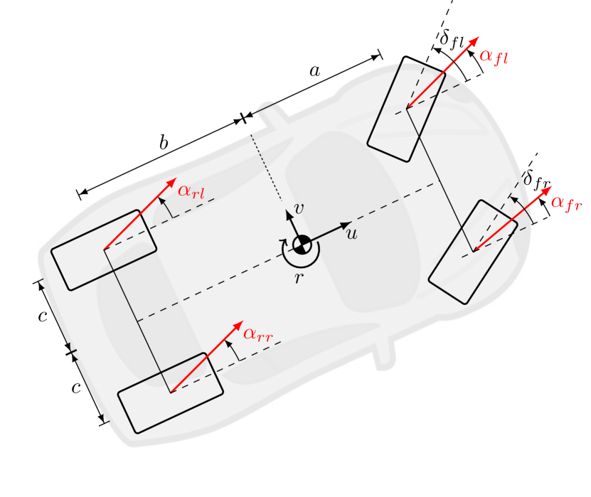
As mentioned, the force generated between the tire and the road is related to the slip angle and it is of fundamental importance for the knowledge of how the lateral forces arise during a curve. The slip angle is the angle between the orientation of the tire and the orientation of the velocity vector of the wheel, as depicted in Fig 1.
The formal definition of slip angle can be derived via kinematic analysis of a planar four-wheel vehicle and is usually defined as:
| (1) |
where and are vehicle longitudinal and lateral velocity components, is the vehicle yaw rate, and are the distances from the vehicle center of gravity to front and rear axles, respectively, and is half of the wheelbase distance. stand for tire steering angles and the subscripts , , and denote quantities corresponding respectively to the front left, front right, rear left and rear right wheels. In the vehicle model sign convention, the steering angle is negative for left turns and positive for right turns.
2.1 Mathematical Formulation
Tire models express the relationship between tire forces and moments with slip ratio and slip angle.
Different mathematical tire models have been developed in the literature. The most widely used model is the semi-empirical tire model introduced by Pacejka pacejka2006tyre , called Pacejka tire model or Magic formula. In a simplified form, the formulation of this tire model for lateral force is as follows:
| (2) |
where D, C, B, E are the Magic formula semi-empirical parameters based on tire measurement data, is the vertical offset of the characteristic curve and is the slip angle.
A second model, known as Dugoff’s tire model, was developed in 1969 by Dugoff et al. dugoff1969tire . In its simplest form, the lateral force is expressed as:
| (3) | ||||
| with | ||||
where is the normal tire load, is the friction coefficient and the cornering stiffness. Conceptually, cornering stiffness is a property of the tire that changes slowly with time due to tire wear, inflation pressure, and temperature fluctuations hsu2009estimation .
Finally, another widespread model is the Brush model pacejka2006tyre , which defines the lateral force as follows:
| (4) | ||||
| where | ||||
Although this article only introduces the most popular and widely used approaches in tire-road friction estimation, there are many valuable studies that have tried to develop new friction models. This subject is addressed in broader texts and books about ground vehicle dynamics such as pacejka2006tyre ; Wong2008theory
The lateral force characteristic curve for each of the presented models is shown in Fig. 2 for several friction coefficients. Initially, the lateral forces increase linearly with the slip angle until it reaches saturation, which represents the tire force limits.
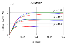
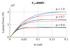

These models show similar behaviors when the slip angle is small. However, they may deviate from each other when high values of vertical force and friction are available. These characteristics suggest that, in the estimation processes, these models could lead to errors due to model discrepancy.
3 Tire-road Friction Identification Through Parametric Regression
As seen in the previous section, the lateral force can be characterized by three fundamental parameters: tire slip angle , normal force and tire-road friction .
When a sufficiently large lateral excitation is detected during a vehicle maneuver, the of road friction estimation can be achieved using the measured signals and the analytical models (2)-(4). This methodology can be seen as a problem of fitting experimental data to a nonlinear analytical function, as addressed in hsu2009estimation ; hsuJournal ; ahn2011robust ; ahnJournal2013 . The method allows the formulation of the problem as one of unconstrained nonlinear least-squares (NLS) optimization.
In other words, we desire to investigate how well we can identify our lateral tire parameters using lateral force information. This requires a good measurement of the lateral tire forces, as well as the knowledge of individual tires. However, if unavailable, the use of an estimate of the axle forces (lumped forces) may hold a lumped friction estimate.
The nonlinear curve-fitting in a least-squares problem consists of finding decision variables that solve the problem:
| (5) | ||||
| (6) |
where is the optimum value that minimizes the objective function, with the parametric function and representing the measured data.
Assuming that the tire analytical models are a good representation of the lateral tire force behavior, they can be used as a parametric function of the NLS method with sets of observed data (in this case, groups of and ).
Despite the promising results of this approach hsuJournal ; ahnJournal2013 , the NLS method has some drawbacks. It requires a long computation time and sometimes this process fails to converge to the true optimal values. The estimator based on NLS generally shows stable estimation results, but does not always guarantee stability and it is difficult to quantify the stability and convergence ahn2011robust . Furthermore, a critical drawback of the NLS is that it is computationally heavy. In a low-speed microprocessor, it may not sustain the same level of performance.
As an alternative to this methodology, we propose solving the problem using neural networks. The theme is approached in a similar form, with the same window of observable data applied in a time-delayed neural network.
4 Estimation of Tire-road Friction Coefficient Using Neural Networks
This section proposes a time delay neural network to detect the TRFC. Two main benefits are expected from this method: firstly, a TDNN can establish network connections and the relationship between input and output instead of storing an entire complex tire model in the controller, which can significantly reduce the computations, guarantee the real time performance and avoid model errors due to model discrepancy; secondly, because the TDNN is trained by measured data, it is able to create a mapping from input parameters to the friction coefficient and accurately capture the temporal structure hidden in the data Zhang2017 .
As the analytical models (2)-(4) show, the lateral force is dependent of , and and these are therefore the parameters selected to feed the neural network. Fig. 3 shows the overall structure used for the TRFC estimation.

Although the existence of tire force sensors, the forces are still hard to measure and the sensors are very expensive. As solution, a Kalman filter variant is used for tire force estimation. Here, we use the approach presented in Cordeiro2016 ; Cordeiro2017 to estimate and using ordinary vehicle sensors, such as GPS, inertial measurement unit (IMU) and encoders.
The observers are developed based on nonlinear vehicle dynamic models with the Extended Kalman Filter (EKF) algorithm. Three estimators are used in a cascade structure to decouple the forces dependency. For vertical forces a 3D vehicle model is used to create a 12-states nonlinear system. For longitudinal and lateral forces the planar vehicle model is used to create two 7-states nonlinear systems. Compromising precision and simplicity, the Dugoff tire model is chosen as the analytical model.
All measures needed for the estimation process are listed in Table 1.
| Signal | Description |
| , , | Vehicle longitudinal, lateral and vertical accelerations |
| u, v, w | Vehicle longitudinal, lateral and vertical linear velocities |
| p, q, r | Vehicle roll, pitch and yaw angular rates |
| Suspension deflection | |
| Tire steering angle |
The aforementioned works about the filter and observer showed that the overall EKF forces estimator is robust against TRFC variations. It turns out that the update stage uses inertial measurements (acceleration) and is capable to correct the forces errors induced by prediction stage. The intuition behind this is that Newton’s second law equations prediction is efficiently corrected by a proper acceleration measurement. Therefore, a constant is applied for the EKF forces estimation.
With this approach the forces are detected individually, which holds the potential of detecting the TRFC independently for each tire. The wheel slip angle is calculated straightforward using (1).
Also, a supplementary consideration should be taken to ensure the algorithm outputs reasonable estimates. Due to sensors noise and the inherent perturbation on lateral forces, and specially on slip angle calculation, the TDNN inputs should be low-pass filtered to prevent the high frequency disturbances from being propagated to the estimate. A unit gain 5 Hz low-pass filter is applied to the estimated forces and slip angle, as shown in Fig. 3.
Before advancing into the learning process of the proposed neural network, it is important to make one addition to the model. When considering the correlation between friction and each tire measure, the correlation coefficient between the normalized lateral force is significantly higher if compared with each force separately, as listed in Table 2. According to (1), the slip angle is determined by vehicle velocities and normal force is mainly affected by the roll over effect. These measures are only affected indirectly by friction, thereby, a low correlation is expected.
| 1.681e-7 | 0.2955 | 1.186e-8 | 0.4076 |
Given this fact, the normalized forces should be selected as one input to feed the neural network instead of and separately. The basis for this choice also lies on the friction circle concept in which the maximum value of the resultant force is determined along a circle (directly influenced by friction), and this value can be decomposed into the limits of the normalized forces Gim1991 .
It is important to note that a positive correlation was observed for positive lateral forces (data obtained from a right hand maneuver). A negative correlation with similar magnitude is expected for negatives forces. The signal, thus, is a consequence of the reference frame.
The TDNN architecture is depicted in Fig. 4. Two inputs were selected: a normalized lateral force , obtained from the kalman estimator, and the calculated slip angle.
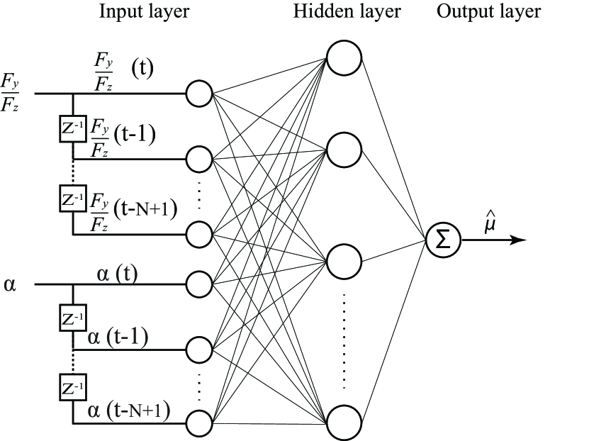
The configuration of the proposed TDNN for TRFC is as follows (see Fig. 4): 2 inputs with 50 samplings delay (observation window of size N = 50) and one single hidden layer with 50 neurons. The neurons differentiable transfer function is nonlinear, properly selected as a Tan-Sigmoid transfer function.
In the neural network data collecting stage, about 200,000 original data are obtained from simulation with a 100 Hz sampling rate. The range of variation of the network input parameters to the tire model is bounded as described in Table 3. The friction coefficient is set with different levels and the vehicle response (data of , and ) is obtained.
| Input parameter | Variation |
| Friction coefficient | 0.3 to 1.2 at intervals of 0.1 |
| Slip angle | [-0.12 0.12] rad |
| Lateral Force | [-2.8 2.8] kN |
| Normal force | [2 4.4] kN |
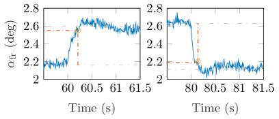
The observation window size was chosen based on the nature of our system. The rise time response due to a change in friction is shown in Fig. 5. The slip angle response (and consequently lateral tire forces, see Fig. 2) shows an average rise time of 0.2 s. In an attempt to capture the vehicle behavior during these transitions, we choose the window size to be approximately double the rising time. Therefore, it is defined N = 50 that corresponds to an observation window of 0.5 seconds.
As in the classical Neural Network, the Time Delay Neural Network also has a training phase. Training was achieved using Matlab Neural Network Toolbox. The Levenberg-Marquardt algorithm is used with 1000 epochs of training iterations with 70% of the collected data randomly taken as the training set, 15% used for validation set and 15% as the test set.
Training phase and further evaluations were carried out on a desktop architecture which features a four-core 4.00 GHz Intel Core i7-6700K Processor, NVIDIA GeForce GTX 950, 32GB of RAM and Ubuntu 16 LTS OS. The system took 7002 seconds to train the aforementioned dataset.
Fig. 6 shows the error residuals of the trained neural network. About 88% of the total data are distributed around zero.
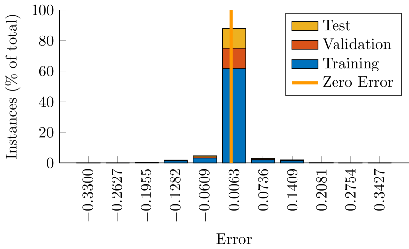
The correlation coefficient (R-value), which is a linear regression between the TDNN predicted values and the targets, and the mean squared error (mse) are shown in Table 4. With R values around 0.94 and 0.95, suggests that the models has a considerable potential of matching the network response to the friction change patterns. Notice also that both R and mse values are close for Training, Validation and Test dataset, which indicates that the network is not overfitting the data.
| R | mse | |
| Training | 0.94355 | 1.0680e-3 |
| Validation | 0.94123 | 1.2597e-3 |
| Test | 0.94059 | 1.3500e-3 |
| Total | 0.94276 | 1.1391e-3 |
5 Results
The simulation results presented in this section are obtained using Matlab/Simulink. A representative and realistic full-vehicle multibody dynamics model (including a steering system, powertrain system, suspension system and the Pacejka tire model for tire ground interactions), was used consisting of the following motions:
-
•
Longitudinal, lateral and vertical body motion;
-
•
Wheels rotation;
-
•
Unsprung masses motion;
-
•
Pitch, roll and yaw body rotation.
The physical parameters of the car used in this study are listed in Table 5. All values are extracted from rafaelcordeirothesis where a complete vehicle modeling and data validation are given. The simulator dynamics is formulated as a 32-states model. The vehicle is configured to simulate a independent rear wheel drive vehicle, providing references of a vehicle state and measured signals. Gaussian noises are added (according to the commercial MTi Xsens sensor specifications (MTi-G-700)) in the simulated measurements to realistically reproduce a real application.
| Parameter name | Value |
| Vehicle mass | 1100 kg |
| Yaw inertia moment | 1350 |
| Roll inertia moment | 337.5 |
| Pitch inertia moment | 1350 |
| Distance from CG to front wheels | 1.5 m |
| Distance from CG to rear wheels | 1.9 m |
| Wheelbase | 1.8 m |
| Wheel rotational inertia | 1 |
| Wheel radius | 0.25 m |
| Height of CG | 0.5 m |
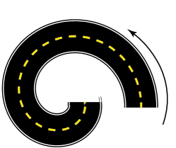
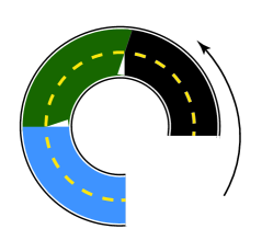
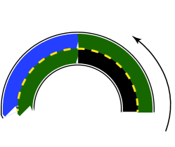
The simulation results of three representative maneuvers are presented here. Table 6 gives the details and purpose of each maneuver. Fig. 7 provides the physical representation of each proposed scenario where the color designates the friction coefficient. The change in friction is time-dependent and occurs at successive time intervals.
During simulation, the system is set on an equilibrium point with constant longitudinal velocity. It is achieved by a PID cruise controller Osman09 . In fact, with constant longitudinal speed, the longitudinal tire forces are reactive with low magnitude and would not have significant impact on lateral forces due coupling effect Hindiyeh09 .
Each case was performed on a different theoretical surface, where a theoretical = 1.0 surface roughly corresponds to driving on a dry pavement, = 0.8 on a wet pavement and = 0.6 corresponds to driving on gravel Wang2004 .
| Simulated Maneuver | Test Surface | Purpose |
| Ramp steer with constant friction coefficient (Fig. 7a) | Constant dry pavement ( = 0.8) | Investigate the early friction sensing ability of the estimator. During the maneuver, lateral forces are gradually increasing, eventually reaching saturation. |
| Constant steer - case 1: step varying for all tires (Fig. 7b) | Five levels of TRFC with unequal steep sizes ( = 1.0 to 0.6) | Determine the estimator response to a quick change in road surface. Friction coefficient is varied at five new levels. |
| Constant steer - case 2: different step varying for left/right tires (Fig. 7c) | Each wheel is subjected simultaneously to two different frictions ( = 0.9, 0.8, = 0.8, 0.7) | Validate the TRFC detection under small friction variations. Also, each wheel is exposed to different surfaces at the same time (distinct for FL and FR tires). |
It is valid to remark that, even though our training and test sets included both left and right turns, due to the symmetry of the system, right turns have a mirror response of left turns that is also included in the network as the result of a data augmentation process.
5.1 Ramp Steer Maneuver
Fig. 8 displays the data resulting from the simulation of a left-hand ramp steer maneuver. The steering angle goes linearly from 0 to -18 degrees at the roadwheels reference.


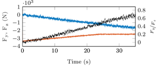

To ensure that there is enough data to be meaningful for the NLS fit and the TDNN approach, first the process is initialized by placing a slip angle threshold . The slip angle data must exceed before the estimation begins, otherwise the fitting optimization may not guarantee a reliable solution.
The TDNN estimator will be here compared with the NLS approach. To show the dependency of the NLS fit with the mathematical model, the regression is performed choosing the Dugoff and Brush models as a parametric function of the nonlinear regression. The window is selected with size and will be used in all cases showed from here on.
Using the estimation algorithm with = 1 degree, the NLS and TDNN algorithm waits until the front tire slip angle exceeds at t = 12 s before fitting the force-slip data (see Fig. 9). The estimated value is the optimum solution of the optimization problem (6) and before instant 12 s the estimation simply holds at initial value .
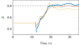

The slight increase in the friction estimate as the maneuver progresses is expected. Initially, during linear tire regime operation, lateral forces measurements have yet to reach their peak value and both methods underestimate the friction coefficient. As more lateral force measurements become available, the peak force limit is reached and the friction estimate reaches a final estimate. Therefore, adequately large slip angles are required for stable and accurate estimation in both TDNN and NLS methods and the slip angle data threshold is indispensable.
The model error also becomes apparent on the NLS fit, where Brush and Dugoff models show different convergence values due to model discrepancy. This divergence arises due to the difference between Pacejka model, used to generate the data, with the models used on the estimators (as discussed in section 2).
5.2 Constant Steer: Case 1
In this setup, the tire-road friction coefficient is set at five levels, varying randomly from 1.0 to 0.6. The transitions occur during successive equal time intervals of 10 seconds. The vehicle is set on an equilibrium point in a constant left turn maneuver. The steering angle of the front left and right tires is set to -18.36 and -15.82 degrees. These values follow the steering Ackerman Geometry. As a consequence, the inner-turn wheel reaches higher tire side slip and lateral force if compared to the outer-turn wheel, as shown in Fig. 10. Also, vertical force is higher on the right tire due to the load transfer. This response appears as a result of the roll over effect measured as a change in vehicle center of mass location relative to the wheels.



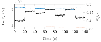

The TRFC estimation results are shown in Fig. 11. One can note the front left estimative is more accurate and less oscillating than the front right estimative. A necessary condition for good estimation results, as shown previously, is a large lateral excitation (high slip angle).
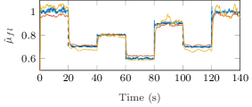
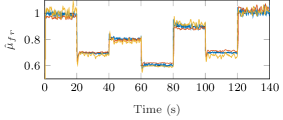

This scenario highlights the dependency of the NLS to the parametric function. The NLS final estimates of each interval show a constant error bias while the TDNN produces a solid and concise estimative. Naturally, there are discrepancies between the dynamic behavior of the real tire system and the derived mathematical model (see Fig. 2). Therefore, a constant error bias should be expected on the NLS model-based approach.
Table 7 displays the root mean square (RMS) error of the estimates of the front left and right tires. Although very similar, a high overall estimation accuracy is achieved for both techniques and it shows great promise for a real implementation.
| Methodology | ||
| TDNN | 0.0346 | 0.0350 |
| 0.0421 | 0.0357 | |
| 0.0546 | 0.0395 |
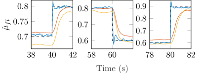
Moreover, the rate of convergence is slightly higher on the TDNN approach. Fig. 12 highlights this response by zooming in Fig. 11a on three intervals of friction transitions. The TDNN estimates converges to a more accurate values with faster responses than the NLS estimates. This behavior lies in the fact that the relationship between input and output was correctly mapped on the database and therefore can be observed on the following results.

5.3 Constant Steer: Case 2
While case 1 showed an equal change for both wheels, here, the tire-road friction coefficient is set at two different levels for each tire. The transition occur during an equal time interval of 10 seconds. Left wheel friction undergoes a transition from 0.9 to 0.8 while right TRFC goes from 0.8 to 0.7.
The vehicle is set on an equilibrium point in a constant left turn maneuver. The knowledge of forces and friction of individual tires is desirable and would offer stability control systems with most needed information. Thus, this change maneuver is conducted to verify that the estimator can identify the friction for each tire individually and certify that the estimation is indeed independent for each wheel.
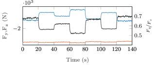
Fig. 13 displays the simulated slip angle, lateral and vertical forces from the proposed right-hand steer maneuver. At instant 10 s, the road surface adhesion coefficient decreases to a different value for each tire. Again, vertical forces are maintained constant due to the maneuver nature, with the changing in friction mostly affecting lateral forces and slip angle.

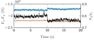


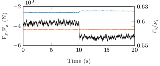

Fig. 14 shows the estimation results. With the TDNN approach, the individual wheel friction is confidently estimated with high accuracy. Since slip angles are larger than for the case 1 scenario, it satisfies the required large lateral forces excitation and gives very accurate estimates. On the NLS estimation results, however, a constant error are still apparent and can be seen during the transitions. This characteristic should be considered when the estimated result is used for control purposes.
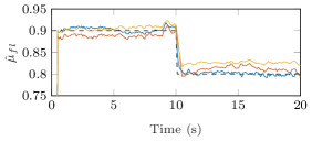
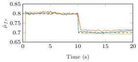

The TDNN shows a slightly better estimation quality, as seen in the RMS error listed in Table 8. Note that the regression based method still exhibits the hindsight bias caused by the inevitable model differences.
| Methodology | ||
| TDNN | 0.0638 | 0.0477 |
| 0.0652 | 0.0493 | |
| 0.0666 | 0.0486 |
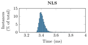
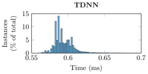
A significant difference in processing time is found when comparing performance and computational efficiency. Fig. 15 shows the normalized histogram of the computation time for both techniques. These values, computed at each time instant, were obtained from 14000 data signals.
It is clear that the computation time of TDNN algorithm is lower than NLS. In summary, TDNN averages 0.594 milliseconds to process the signal (corresponding to one iteration) compared to 3.379 milliseconds of the NLS. This has the potential to allow a higher sample frequency of the complete system.
6 Conclusions
In this study, we presented a hierarchical TRFC estimation method based on a time delay neural network and compared it with a classical nonlinear regression approach, using the same data observation window. The overall estimation algorithm was evaluated on varying road surfaces with three different scenarios. A high-fidelity and realistic full-vehicle multibody dynamics model for Matlab/Simulink platform was used in the simulations.
Although road-friction was accurately identified using both algorithms, there is a primary shortcoming in the presented lateral-force based friction estimation: it requires sufficient levels of lateral excitation for the correct friction identification. An earlier knowledge of the TRFC is desirable, however, both approaches showed a similar behavior: a necessary waiting time for the tire slip angle to fulfill the observation window satisfying the specified excitation threshold.
Nonetheless, as an algebraic methods, the NLS method relies more heavily on an accurate model which may be a source for estimation errors. Indeed, the NLS needs a prespecified parametric function for precise tunning parameters and, as a consequence, stationary estimation errors may be expected if the given function is not adequate.
On the other hand, the TDNN method is independent of any mathematical tire model, however, requires a sufficient and representative database. In this study, the TDNN was also able to provide estimates with lower RMS errors compared with the classical regression approach. It also demands less computation time at each time instant and may be the best alternative for a real time implementation in embedded systems.
Since the proposed method is only analyzed theoretically and validated via simulation, an actual benchmark or field test is needed in the subsequent work to verify the proposed approach. Future works may also include the design of a time delay neural network containing not only lateral information but also longitudinal forces, slip ratio and self-moment align.
Acknowledgements.
This work was supported by FCT Portugal, through IDMEC under projects LAETA (UID/EMS/ 50022/2019). The mobility of A. Ribeiro has been possible with the Erasmus Mundus SMART2 support (Project Reference: 552042-EM-1-2014-1-FR-ERA MUNDUS-EMA2) coordinated by CENTRALESUPELEC. The authors also acknowledge the support of FAPESP through Regular project AutoVERDE N. 2018/04905-1, Ph.D. FAPESP 2018/05712-2 and CNPq grant 305600/2017-6.References
- [1] Kanwar Bharat Singh and Saied Taheri. Estimation of tire–road friction coefficient and its application in chassis control systems. Systems Science & Control Engineering, 3(1):39–61, December 2014.
- [2] Liang Shao, Chi Jin, Cornelia Lex, and Arno Eichberger. Robust road friction estimation during vehicle steering. Vehicle System Dynamics, 57(4):493–519, 2019.
- [3] Yung-Hsiang J Hsu, Shad Laws, Christopher D Gadda, and J Christian Gerdes. A method to estimate the friction coefficient and tire slip angle using steering torque. In ASME 2006 International Mechanical Engineering Congress and Exposition, pages 515–524. American Society of Mechanical Engineers, 2006.
- [4] Ali I. H. Al-Zughaibi. Experimental and analytical investigations of friction at lubricant bearings in passive suspension systems. Nonlinear Dynamics, 94(2):1227–1242, Oct 2018.
- [5] Chang Sun Ahn. Robust estimation of road friction coefficient for vehicle active safety systems. PhD thesis, University of Michigan, 2011.
- [6] R. de Castro, R. E. Araujo, J. S. Cardoso, and D. Freitas. A new linear parametrization for peak friction coefficient estimation in real time. In 2010 IEEE Vehicle Power and Propulsion Conference, pages 1–6, Sep. 2010.
- [7] W. R. Pasterkamp and H. B. Pacejka. The tyre as a sensor to estimate friction. Vehicle System Dynamics, 27(5-6):409–422, jun 1997.
- [8] Yung-Hsiang Judy Hsu. Estimation and control of lateral tire forces using steering torque. PhD thesis, Stanford University, 2009.
- [9] Y.-H Judy Hsu, Shad M. Laws, and J Christian Gerdes. Estimation of tire slip angle and friction limits using steering torque. 18:896 – 907, 08 2010.
- [10] Changsun Ahn, Huei Peng, and Hongtei Eric Tseng. Robust estimation of road frictional coefficient. IEEE Transactions on Control Systems Technology, 21(1):1–13, 2013.
- [11] Steffen Müller, Michael Uchanski, and Karl Hedrick. Estimation of the maximum tire-road friction coefficient. Journal of Dynamic Systems, Measurement, and Control, 125(4):607, 2003.
- [12] T. Hsiao, N. C. Liu, and S. Y. Chen. Robust estimation of the friction forces generated by each tire of a vehicle. In Proceedings of the 2011 American Control Conference, pages 5261–5266, June 2011.
- [13] R. Rajamani, G. Phanomchoeng, D. Piyabongkarn, and J. Y. Lew. Algorithms for real-time estimation of individual wheel tire-road friction coefficients. IEEE/ASME Transactions on Mechatronics, 17(6):1183–1195, Dec 2012.
- [14] K Li, J A Misener, and K Hedrick. On-board road condition monitoring system using slip-based tyre-road friction estimation and wheel speed signal analysis. Proceedings of the Institution of Mechanical Engineers, Part K: Journal of Multi-body Dynamics, 221(1):129–146, 2007.
- [15] Zhiquan Qi, Saied Taheri, Baofeng Wang, and Hongxiao Yu. Estimation of the tyre–road maximum friction coefficient and slip slope based on a novel tyre model. Vehicle System Dynamics, 53(4):506–525, 2015.
- [16] X. Xia, L. Xiong, K. Sun, and Z. P. Yu. Estimation of maximum road friction coefficient based on lyapunov method. International Journal of Automotive Technology, 17(6):991–1002, Dec 2016.
- [17] J. Casselgren, M. Sjodahl, S. Woxneryd, and M. Sanfridsson. Classification of road conditions – to improve safety. In 11th International Forum on Advanced Microsystems for Automotive Applications, pages 47–59. Springer Science Business Media, 2007.
- [18] A.J; Tuononen. Optical position detection to measure tyre carcass deflections. Vehicle System Dynamics, 46(6):471–481, 2008.
- [19] M. Jokela, M. Kutila, and L. Le. Road condition monitoring system based on a stereo camera. In 2009 IEEE 5th International Conference on Intelligent Computer Communication and Processing, pages 423–428, Aug 2009.
- [20] Patrik Jonsson. Classification of road conditions: From camera images and weather data. In International Conference on Computational Intelligence for Measurement Systems and Applications (CIMSA) Proceedings. Institute of Electrical and Electronics Engineers (IEEE), sep 2011.
- [21] Long Chen, Mingyuan Bian, Yugong Luo, Zhaobo Qin, and Keqiang Li. Tire–road friction coefficient estimation based on the resonance frequency of in-wheel motor drive system. Vehicle System Dynamics, 54(1), nov 2015.
- [22] Long Chen, Yugong Luo, Mingyuan Bian, Zhaobo Qin, Jian Luo, and Keqiang Li. Estimation of tire-road friction coefficient based on frequency domain data fusion. Mechanical Systems and Signal Processing, 85:177–192, aug 2016.
- [23] W.R. Pasterkamp and H.B. Pacejka. Optimal design of neural networks for estimation of tyre/road friction. Vehicle System Dynamics, 29(sup1):312–321, jan 1998.
- [24] Jadranko Matuško, Ivan Petrović, and Nedjeljko Perić. Neural network based tire/road friction force estimation. Engineering Applications of Artificial Intelligence, 21(3):442–456, April 2008.
- [25] Arash Zareian, Shahram Azadi, and Reza Kazemi. Estimation of road friction coefficient using extended kalman filter, recursive least square, and neural network. Proceedings of the Institution of Mechanical Engineers, Part K: Journal of Multi-body Dynamics, 230(1):52–68, May 2015.
- [26] Xudong Zhang and Dietmar Göhlich. A hierarchical estimator development for estimation of tire-road friction coefficient. PLOS ONE, 12(2):e0171085, feb 2017.
- [27] G. Panahandeh, E. Ek, and N. Mohammadiha. Road friction estimation for connected vehicles using supervised machine learning. In 2017 IEEE Intelligent Vehicles Symposium (IV), pages 1262–1267, June 2017.
- [28] Sohini Roychowdhury, Minming Zhao, Andreas Wallin, Niklas Ohlsson, and Mats Jonasson. Machine learning models for road surface and friction estimation using front-camera images. In 2018 International Joint Conference on Neural Networks (IJCNN). IEEE, July 2018.
- [29] Guangwei Yang, Qiang Joshua Li, You Zhan, Yue Fei, and Aonan Zhang. Convolutional neural network–based friction model using pavement texture data. Journal of Computing in Civil Engineering, 32(6):04018052, November 2018.
- [30] Yuchuan Du, Chenglong Liu, Yang Song, Yishun Li, and Yu Shen. Rapid estimation of road friction for anti-skid autonomous driving. IEEE Transactions on Intelligent Transportation Systems, pages 1–10, 2019.
- [31] Fei Wu, Leibny Paola García-Perera, Daniel Povey, and Sanjeev Khudanpur. Advances in automatic speech recognition for child speech using factored time delay neural network. In Proc. Interspeech 2019, pages 1–5, 2019.
- [32] Sarah A Saruchi, Mohd HM Ariff, Hairi Zamzuri, Nurhaffizah Hassan, and Nurbaiti Wahid. Modeling of occupant’s head movement behavior in motion sickness study via time delay neural network. SIMULATION, 2019.
- [33] Triwiyanto, O. Wahyunggoro, H. A. Nugroho, and Herianto. Time delay neural network to estimate the elbow joint angle based on electromyography. In 2018 2nd International Conference on Biomedical Engineering (IBIOMED), pages 100–105, July 2018.
- [34] N. Ashwini, M. Rajshekar Patil, and Manoj Kumar Singh. Computational intelligence based chaotic time series prediction using evolved neural network. In Vikrant Bhateja, Carlos A. Coello Coello, Suresh Chandra Satapathy, and Prasant Kumar Pattnaik, editors, Intelligent Engineering Informatics, pages 383–396. Springer, 2018.
- [35] Hans B. Pacejka. Tyre and vehicle dynamics. Butterworth-Heinemann, Oxford, second edition, 2006.
- [36] Howard Dugoff, Paul S Fancher, and Leonard Segel. Tire performance characteristics affecting vehicle response to steering and braking control inputs. Technical Report Contract CST-460, Office of Vehicle Systems Research, August 1969.
- [37] Jo Yung Wong. Theory of Ground Vehicles. Wiley, Hoboken, N.J, third edition, 2008.
- [38] Rafael A. Cordeiro, Alessandro C. Victorino, Paulo A.V. Ferreira, Ely C. de Paiva, and Samuel S. Bueno. Tire-ground forces estimation in a 4-wheel vehicle using a delayed interconnected cascade-observer structure. IFAC-PapersOnLine, 49(15):139–144, 2016.
- [39] Rafael A. Cordeiro, Alexandre M. Ribeiro, Joze R. Oliveira, Alessandro C. Victorino, Paulo A.V. Ferreira, Ely C. de Paiva, and Samuel S. Bueno. Road grades and tire forces estimation using two-stage extended kalman filter in a delayed interconnected cascade structure. IEEE Intelligent Vehicles Symposium, 2017.
- [40] G. Gim and P. E. Nikravesh. An analytical model of pneumatic tyres for vehicle dynamic simulations. part 2: Comprehensive slips. International Journal of Vehicle Design, 12(1):19–39, 1991.
- [41] Rafael de Angelis Cordeiro. Track control of a four-wheel robotic vehicle in adverse terrain conditions. PhD thesis, Universidade Estadual de Campinas, 2017.
- [42] K. Osman, M. F. Rahmat, and M. A. Ahmad. Modelling and controller design for a cruise control system. In 2009 5th International Colloquium on Signal Processing Its Applications, pages 254–258, March 2009.
- [43] Rami Y. Hindiyeh and J. Christian Gerdes. Equilibrium analysis of drifting vehicles for control design. volume ASME 2009 Dynamic Systems and Control Conference, Volume 1 of Dynamic Systems and Control Conference, pages 181–188, 2009.
- [44] Junmin Wang, Lee Alexander, and Rajesh Rajamani. Friction estimation on highway vehicles using longitudinal measurements. Journal of Dynamic Systems, Measurement, and Control, 126(2):265, 2004.