Goal-oriented error estimation and adaptivity in MsFEM computations

Ludovic Chamoin ludovic.chamoin@ens-paris-saclay.fr Frédéric Legoll frederic.legoll@enpc.fr LMT (ENS Paris-Saclay, CNRS, Université Paris-Saclay), 61 avenue du Président Wilson, 94235 Cachan, France Inria Paris, MATHERIALS project-team, 2 rue Simone Iff, CS 42112, 75589 Paris Cedex 12, France Laboratoire Navier (ENPC, Paris-Est University), 6-8 avenue Blaise Pascal, 77455 Marne-La-Vallée Cedex 2, France
Résumé

We introduce a goal-oriented strategy for multiscale computations performed using the Multiscale Finite Element Method (MsFEM). In a previous work, we have shown how to use, in the MsFEM framework, the concept of Constitutive Relation Error (CRE) to obtain a guaranteed and fully computable a posteriori error estimate in the energy norm (as well as error indicators on various error sources). Here, the CRE concept is coupled with the solution of an adjoint problem to control the error and drive an adaptive procedure with respect to a given output of interest. Furthermore, a local and non-intrusive enrichment technique is proposed to enhance the accuracy of error bounds. The overall strategy, which is fully automatic and robust, enables to reach an appropriate trade-off between certified reliability and computational cost in the MsFEM context. The performances of the proposed method are investigated on several illustrative numerical test cases. In particular, the error estimation is observed to be very accurate, yielding a very efficient adaptive procedure.

keywords:
Multiscale problems , MsFEM approach , A posteriori error estimation , Goal-oriented , Adaptivity
MSC:
[2010] 35Q74 , 65N15 , 74S05

1 Introduction and objectives

Highly heterogeneous materials are ubiquitous in Material Sciences and Computational Mechanics. Examples include porous or perforated media, composite materials, …Developing multiscale numerical methods to simulate the (thermal, mechanical, …) response of such materials is an increasingly active research field. As an alternative to solving a full fine-scale problem (the cost of which is usually prohibitively expensive), multiscale modeling aims at linking the different scales by appropriately capturing the effect of the smaller scales on the larger scales. This enables an accurate description of complex physical phenomena and/or the prediction of macroscopic properties at a limited computational cost. In the recent years, significant progress has been witnessed in the design of multiscale methods for elliptic PDEs that take into account scale separation between macroscopic and microscopic features. We can distinguish two families of multiscale methods. The first family includes approaches relying on multilevel finite elements, such as HMM or FE2 methods [22, 26]. They perform a numerical homogenization of the medium in order to find local effective material properties, which are next inserted in a global macroscopic problem which can be handled with a reduced number of degrees of freedom. Such approaches can be considered as numerical generalizations of classical homogenization approaches (see e.g. [9]) to non-periodic media. The second family includes approaches based on superposition of scales, such as the GFEM [64], the MsFEM [33], the LOD [51] and the VMS [36] methods, to name but a few. In this work, we focus on the Multiscale Finite Element Method (MsFEM) which has been the object of numerous research works (see [24] for an overview). This method is based on the classical FEM framework, defining an approximate solution in a finite dimension space related to a macroscopic mesh, but uses specific basis functions which encode fine-scale details. The basis functions are obtained, in a preliminary offline stage, by solving fine-scale equations over local subdomains. The MsFEM approximation is next computed during an inexpensive online stage, and provides a numerical approximation that describes details of the exact solution at different scales, including the small ones.

A recurring concern when using multiscale methods is the control of the accuracy of the numerical solution. In particular, it is critical to understand, quantify and control how errors generated by different sources and at different scales affect the overall error, in order to build relevant adaptive strategies and focus the computational efforts where they are required. Following the large literature on a posteriori error estimation in the monoscale framework of the Finite Element Method (FEM) (see e.g. [67, 3] for classical textbooks and [18] for a recent review), several verification tools have been developed for multiscale methods [65, 44, 45, 52, 1, 37, 2, 31, 20]. However, many open questions remain, such as quantitative assessment of error propagation across scales, relevant adaptive strategies, …Recently, we have proposed a robust a posteriori error estimation tool for MsFEM computations [19]. It uses the concept of Constitutive Relation Error (CRE), which has been developed in the Computational Mechanics community for more than thirty years [42]. It enables both (i) to derive fully computable (i.e. without any unknown multiplicative constant) and guaranteed bounds on the global error measured in the energy norm, which may further be used as stopping criteria in adaptive algorithms, from an extension of the CRE to the multiscale context, and (ii) to assess the various MsFEM error sources and drive an adaptive algorithm from local error maps in order to reach a prescribed error tolerance.

In the present article, we extend the methodology introduced in [19] to a posteriori goal-oriented error estimation, namely the control of the error on specific scalar-valued outputs of interest for problems discretized with MsFEM. In this specific context, material heterogeneities may indeed require standard adaptive methods to add degrees of freedom in regions with limited influence on the output of interest, or not to add some in regions which significantly affect this output. Consequently, alternative a posteriori error estimation and adaptivity methods need to be introduced, taking into account the specific quantities of interest of the problem. For that purpose, we introduce classical duality arguments along with an adjoint problem [6, 59, 63, 21, 62, 53, 29, 16], which enable to target the error estimation and adaptivity procedure towards the approximation of the considered quantity of interest. We also use strategies to bound the error that are similar to those employed for monoscale applications with CRE [38, 17, 39, 58, 68, 43]. In particular, we introduce a non-intrusive approach for the approximate solution of the adjoint solution (using so-called handbook functions), which enables to obtain both guaranteed and sharp error bounds. We also define local indicators on various error sources (coarse mesh size, size of the local fine meshes, …) in order to drive the adaptive strategy, and automatically and iteratively select optimal MsFEM parameters to be used locally for reducing the error in the goal functional. In order to comply with the MsFEM philosophy and the multi-query paradigm, all additional costly computations associated with the proposed procedures are performed in the offline stage. The overall verification tool enables to perform MsFEM computations in which: (i) a given precision on specified outputs of interest is attained at the end of the simulation; (ii) the computational work which is needed is as small as possible. The proposed approach, devoted to the Multiscale Finite Element Method and which fulfills the above two objectives, is an alternative to the goal-oriented adaptive strategy recently proposed in [20] within the Generalized Multiscale Finite Element framework, which uses residual-based techniques and which mainly focuses on goal-oriented adaptivity alone. We also mention the approach [44] proposed in the VMS framework, and the approach [50] proposed in the HMM framework where the overall error is also split between different contributions each related to a discretization parameter.

The performances of our approach are evaluated on several numerical examples. It is interesting to note that it leads in practice to MsFEM computations with guaranteed prescribed accuracy, and in which fine-scale features of the solution are required (and captured using fine discretization parameters) only in very localized parts of the physical domain. A limited accuracy of the fine scale computations is thus sufficient. Consequently, it naturally and automatically shares some resemblance with alternative multiscale computing strategies based on local enrichments or couplings between fine-scale and coarser-scale (upscaled) models [48, 8, 15, 28, 49], these strategies being associated to modeling error estimation [57, 56, 66, 54, 61, 4].

This article is organized as follows. In Section 2, we introduce the model problem we consider along with basic notions on the MsFEM discretization approach. The CRE concept applied to the MsFEM framework is recalled in Section 3. In Section 4, we extend this concept to goal-oriented error estimation within MsFEM computations. This is the core of this work. An associated adaptive strategy, enabling to control the accuracy of outputs of interest, is introduced in Section 5. We discuss several illustrative numerical experiments in Section 6. Eventually, conclusions and perspectives are collected in Section 7.

2 Model problem and MsFEM approximation

To start with, we describe our model problem in Section 2.1. In Section 2.2, we next recall some basic elements on several variants of MsFEM: the initial conforming variant, the oversampling variant (see Section 2.2.3) and the higher-order variant introduced by G. Allaire and R. Brizzi (see Section 2.2.4). The reader familiar with MsFEM may easily skip Section 2.2 and directly proceed to the a posteriori error estimation strategy described in Section 3.

2.1 Model problem

We consider mathematical models described by partial differential equations (PDEs) and characterized by multiscale material heterogeneities. For the sake of simplicity, we focus on the following elliptic problem posed on some open and bounded domain ΩdΩsuperscript𝑑\Omega\subset\mathbb{R}^{d}:

(𝔸εuε)=fin Ω,uε=0on ΓD,𝔸εuε𝒏=gon ΓN.formulae-sequencebold-∇superscript𝔸𝜀bold-∇superscript𝑢𝜀𝑓in Ωformulae-sequencesuperscript𝑢𝜀0on ΓDsuperscript𝔸𝜀bold-∇superscript𝑢𝜀𝒏𝑔on ΓN-\boldsymbol{\nabla}\cdot(\mathbb{A}^{\varepsilon}\boldsymbol{\nabla}u^{\varepsilon})=f\ \ \text{in $\Omega$},\qquad u^{\varepsilon}=0\ \ \text{on $\Gamma_{D}$},\qquad\mathbb{A}^{\varepsilon}\boldsymbol{\nabla}u^{\varepsilon}\cdot\boldsymbol{n}=g\ \ \text{on $\Gamma_{N}$}. (1)

The boundary Γ=ΩΓΩ\Gamma=\partial\Omega is split into a subset ΓDΩsubscriptΓ𝐷Ω\Gamma_{D}\subset\partial\Omega (with measure |ΓD|>0subscriptΓ𝐷0|\Gamma_{D}|>0) where homogeneous Dirichlet boundary conditions are applied, and a subset ΓN=ΩΓDΩsubscriptΓ𝑁ΩsubscriptΓ𝐷Ω\Gamma_{N}=\partial\Omega\setminus\Gamma_{D}\subset\partial\Omega where Neumann boundary conditions are applied. We assume that fL2(Ω)𝑓superscript𝐿2Ωf\in L^{2}(\Omega) and gL2(ΓN)𝑔superscript𝐿2subscriptΓ𝑁g\in L^{2}(\Gamma_{N}), corresponding to body and traction loadings respectively, are slowly varying functions. The quantity 𝒒ε=𝔸εuεsuperscript𝒒𝜀superscript𝔸𝜀bold-∇superscript𝑢𝜀\boldsymbol{q}^{\varepsilon}=\mathbb{A}^{\varepsilon}\boldsymbol{\nabla}u^{\varepsilon} is the flux associated to uεsuperscript𝑢𝜀u^{\varepsilon} through the constitutive relation.

The second-order diffusion tensor 𝔸ε(L(Ω))d×dsuperscript𝔸𝜀superscriptsuperscript𝐿Ω𝑑𝑑\mathbb{A}^{\varepsilon}\in(L^{\infty}(\Omega))^{d\times d} is a heterogeneous object, with rapid oscillations and possibly high contrast. The parameter ε𝜀\varepsilon refers to the typical (presumably small) length scale of the heterogeneities. We assume that 𝔸εsuperscript𝔸𝜀\mathbb{A}^{\varepsilon} is a symmetric matrix that is uniformly elliptic and bounded, in the sense that there exist α>0𝛼0\alpha>0 and β>0𝛽0\beta>0 such that

ε0,𝝃d,α|𝝃|2𝔸ε(𝒙)𝝃𝝃β|𝝃|2a.e. in Ω.formulae-sequenceformulae-sequencefor-all𝜀0formulae-sequencefor-all𝝃superscript𝑑𝛼superscript𝝃2superscript𝔸𝜀𝒙𝝃𝝃𝛽superscript𝝃2a.e. in Ω.\forall\varepsilon\geq 0,\ \ \forall\boldsymbol{\xi}\in\mathbb{R}^{d},\quad\alpha|\boldsymbol{\xi}|^{2}\leq\mathbb{A}^{\varepsilon}(\boldsymbol{x})\boldsymbol{\xi}\cdot\boldsymbol{\xi}\leq\beta|\boldsymbol{\xi}|^{2}\quad\text{a.e. in $\Omega$.}

Introducing the functional space V={v1(Ω),v=0 on ΓD}𝑉𝑣superscript1Ωv=0 on ΓDV=\{v\in\mathcal{H}^{1}(\Omega),\ \ \text{$v=0$ on $\Gamma_{D}$}\}, the weak formulation of (1) consists in finding uεVsuperscript𝑢𝜀𝑉u^{\varepsilon}\in V such that

vV,Bε(uε,v)=F(v)formulae-sequencefor-all𝑣𝑉superscript𝐵𝜀superscript𝑢𝜀𝑣𝐹𝑣\forall v\in V,\quad B^{\varepsilon}(u^{\varepsilon},v)=F(v) (2)

with

Bε(u,v)=Ω𝔸εuv,F(v)=Ωfv+ΓNgv.formulae-sequencesuperscript𝐵𝜀𝑢𝑣subscriptΩsuperscript𝔸𝜀bold-∇𝑢bold-∇𝑣𝐹𝑣subscriptΩ𝑓𝑣subscriptsubscriptΓ𝑁𝑔𝑣B^{\varepsilon}(u,v)=\int_{\Omega}\mathbb{A}^{\varepsilon}\boldsymbol{\nabla}u\cdot\boldsymbol{\nabla}v,\qquad F(v)=\int_{\Omega}f\,v+\int_{\Gamma_{N}}g\,v.

The bilinear form Bεsuperscript𝐵𝜀B^{\varepsilon} is symmetric, continuous and coercive on V𝑉V. It thus defines an inner product and induces the energy norm |v|=Bε(v,v)norm𝑣superscript𝐵𝜀𝑣𝑣{\left|\kern-1.07639pt\left|\kern-1.07639pt\left|v\right|\kern-1.07639pt\right|\kern-1.07639pt\right|}=\sqrt{B^{\varepsilon}(v,v)} on V𝑉V. The 1superscript1\mathcal{H}^{1}-norm is denoted 1\|\cdot\|_{1}, and it is equivalent to the norm ||||||{\left|\kern-1.07639pt\left|\kern-1.07639pt\left|\,\cdot\,\right|\kern-1.07639pt\right|\kern-1.07639pt\right|} on V𝑉V.

The model problem (2) may be numerically solved using classical and direct numerical techniques, such as the finite element method (FEM). In this method, a conforming partition 𝒯Hsubscript𝒯𝐻\mathcal{T}_{H} of ΩΩ\Omega is introduced (H𝐻H denotes the characteristic size of the elements of 𝒯Hsubscript𝒯𝐻\mathcal{T}_{H}) and a finite dimensional space VH0Vsuperscriptsubscript𝑉𝐻0𝑉V_{H}^{0}\subset V is constructed from Lagrange basis functions ϕi0superscriptsubscriptitalic-ϕ𝑖0\phi_{i}^{0} associated with each node i𝑖i of 𝒯Hsubscript𝒯𝐻\mathcal{T}_{H}. The solution to (2) is thus approximated by uH=iuiϕi0VH0subscript𝑢𝐻subscript𝑖subscript𝑢𝑖superscriptsubscriptitalic-ϕ𝑖0superscriptsubscript𝑉𝐻0\displaystyle u_{H}=\sum_{i}u_{i}\,\phi_{i}^{0}\in V_{H}^{0}, solution to

vVH0,Bε(uH,v)=F(v).formulae-sequencefor-all𝑣subscriptsuperscript𝑉0𝐻superscript𝐵𝜀subscript𝑢𝐻𝑣𝐹𝑣\forall v\in V^{0}_{H},\quad B^{\varepsilon}(u_{H},v)=F(v).

A very fine mesh is necessary to represent the multiscale nature of the solution uεsuperscript𝑢𝜀u^{\varepsilon}. This leads to choosing H<ε𝐻𝜀H<\varepsilon, and thus a prohibitively large number of degrees of freedom. The resulting method has a too high computational complexity.

As an alternative, multiscale model reduction techniques based on a scale separation assumption are typically used to solve (2) accurately and efficiently. On the one hand, homogenization strategies can be employed when the structure of 𝔸εsuperscript𝔸𝜀\mathbb{A}^{\varepsilon} is periodic (or locally periodic, or random and stationary, …; see [9]), or when one is only interested in macroscopic/upscaled properties of the model (1) (we refer e.g. to [22, 26]). On the other hand, multiscale numerical approaches have the capability to approximate, efficiently and for general structures of 𝔸εsuperscript𝔸𝜀\mathbb{A}^{\varepsilon}, the details of uεsuperscript𝑢𝜀u^{\varepsilon} at all scales. In the following, we focus on the Multiscale Finite Element Method (MsFEM) [33, 24, 46], which is one of these latter approaches.

2.2 MsFEM approximation

2.2.1 General strategy

We define two partitions of ΩΩ\Omega: (i) a coarse grid partition 𝒯Hsubscript𝒯𝐻\mathcal{T}_{H}, referred to as the macro mesh; (ii) a fine grid partition 𝒯hsubscript𝒯\mathcal{T}_{h}, subordinate to 𝒯Hsubscript𝒯𝐻\mathcal{T}_{H}, referred to as the micro mesh (the mesh size hh is chosen smaller, and often much smaller, than H𝐻H). The mesh 𝒯hsubscript𝒯\mathcal{T}_{h} is in practice obtained by refining each coarse element of 𝒯Hsubscript𝒯𝐻\mathcal{T}_{H}. It should be chosen so that oscillations of the data can be accurately captured on 𝒯hsubscript𝒯\mathcal{T}_{h}.

The main idea in the MsFEM approach is to construct a set {ϕiε}superscriptsubscriptitalic-ϕ𝑖𝜀\{\phi_{i}^{\varepsilon}\} of multiscale basis functions, associated with each node i𝑖i of the macro mesh 𝒯Hsubscript𝒯𝐻\mathcal{T}_{H}, which encode fine scale information and local heterogeneities of the solution space. These are constructed locally, in an offline phase, as the solutions, over each element K𝐾K of the coarse mesh (or over a local region SKK𝐾subscript𝑆𝐾S_{K}\supset K), to problems of the form

(𝔸εϕiε)=0in K,bold-∇superscript𝔸𝜀bold-∇superscriptsubscriptitalic-ϕ𝑖𝜀0in K\boldsymbol{\nabla}\cdot(\mathbb{A}^{\varepsilon}\boldsymbol{\nabla}\phi_{i}^{\varepsilon})=0\quad\text{in $K$}, (3)

complemented with boundary conditions discussed below. We notice that the local problems (3) are decoupled one from each other. They are thus well-suited to parallel computations. Furthermore, they do not depend on the loads f𝑓f and g𝑔g, which is a main advantage in a multi-query context. These local problems are in practice solved numerically using the micro mesh 𝒯hsubscript𝒯\mathcal{T}_{h}.

Remark 1

A variant in the construction of multiscale basis functions, referred to as the Generalized Multiscale Finite Element Method (GMsFEM), was recently introduced in [23]. It consists in defining a larger number of basis functions over each element K𝐾K of 𝒯Hsubscript𝒯𝐻\mathcal{T}_{H}, which are obtained using local spectral problems.

Once the multiscale basis functions are computed, a classical Galerkin approximation of (2) is performed on the finite dimensional space VHε=Span{ϕiε}subscriptsuperscript𝑉𝜀𝐻Spansuperscriptsubscriptitalic-ϕ𝑖𝜀V^{\varepsilon}_{H}=\text{Span}\{\phi_{i}^{\varepsilon}\}. The solution to (2) is thus approximated by some uHε=iuiϕiεVHεsubscriptsuperscript𝑢𝜀𝐻subscript𝑖subscript𝑢𝑖superscriptsubscriptitalic-ϕ𝑖𝜀superscriptsubscript𝑉𝐻𝜀\displaystyle u^{\varepsilon}_{H}=\sum_{i}u_{i}\,\phi_{i}^{\varepsilon}\in V_{H}^{\varepsilon}, defined as the solution (computed during the online phase) to the following global problem:

vVHε,Bε(uHε,v)=F(v).formulae-sequencefor-all𝑣subscriptsuperscript𝑉𝜀𝐻superscript𝐵𝜀subscriptsuperscript𝑢𝜀𝐻𝑣𝐹𝑣\forall v\in V^{\varepsilon}_{H},\quad B^{\varepsilon}(u^{\varepsilon}_{H},v)=F(v). (4)

We note that VHεsuperscriptsubscript𝑉𝐻𝜀V_{H}^{\varepsilon} and VH0superscriptsubscript𝑉𝐻0V_{H}^{0} share the same dimension. The above problem hence involves a limited number of degrees of freedom. The small scale information incorporated in the basis functions ϕiεsuperscriptsubscriptitalic-ϕ𝑖𝜀\phi_{i}^{\varepsilon} is thus brought to the large scales through couplings in the global stiffness matrix. The assembly of this matrix is inexpensive since it reuses local matrices computed and stored in the offline stage.

The MsFEM approach leads to a considerable decrease in memory requirements and CPU cost as an accurate approximation may be obtained for Hεmuch-greater-than𝐻𝜀H\gg\varepsilon. Nevertheless, a posteriori error estimates and adaptive techniques are required to ensure a sufficiently high-fidelity approximation at a limited cost. These are addressed in Sections 3 and 4.

2.2.2 Conforming MsFEM

The choice of the boundary conditions for the local problems (3) (when constructing the multiscale basis functions) is of critical importance, since it can significantly affect the accuracy of the MsFEM solution. A first choice, leading to a conforming numerical discretization, is to impose an affine evolution of ϕiεsuperscriptsubscriptitalic-ϕ𝑖𝜀\phi_{i}^{\varepsilon} along K𝐾\partial K. Introducing the classical first-order and piecewise affine FE basis functions ϕi0superscriptsubscriptitalic-ϕ𝑖0\phi_{i}^{0}, we thus consider the local problems

(𝔸εϕiε)=0in K,ϕiε=ϕi0on K.formulae-sequencebold-∇superscript𝔸𝜀bold-∇superscriptsubscriptitalic-ϕ𝑖𝜀0in Ksuperscriptsubscriptitalic-ϕ𝑖𝜀superscriptsubscriptitalic-ϕ𝑖0on K\boldsymbol{\nabla}\cdot(\mathbb{A}^{\varepsilon}\boldsymbol{\nabla}\phi_{i}^{\varepsilon})=0\quad\text{in $K$},\qquad\phi_{i}^{\varepsilon}=\phi_{i}^{0}\quad\text{on $\partial K$}. (5)

In the regime of interest Hε𝐻𝜀H\geq\varepsilon, assuming that 𝔸εsuperscript𝔸𝜀\mathbb{A}^{\varepsilon} has a periodic structure (i.e. 𝔸ε=𝔸per(/ε)\mathbb{A}^{\varepsilon}=\mathbb{A}^{\rm per}(\cdot/\varepsilon) for some fixed matrix 𝔸persuperscript𝔸per\mathbb{A}^{\rm per}) and that the local problems (5) are solved exactly (and under some technical regularity assumptions), the following a priori error estimate holds [34]:

uεuHε1C(H+εH+ε),subscriptnormsuperscript𝑢𝜀subscriptsuperscript𝑢𝜀𝐻1𝐶𝐻𝜀𝐻𝜀\|u^{\varepsilon}-u^{\varepsilon}_{H}\|_{1}\leq C\left(H+\sqrt{\frac{\varepsilon}{H}}+\sqrt{\varepsilon}\right), (6)

where the constant C𝐶C is independent of ε𝜀\varepsilon and H𝐻H. This estimate is derived using the periodic homogenization theory that provides (when ε1much-less-than𝜀1\varepsilon\ll 1) a detailed description of uεsuperscript𝑢𝜀u^{\varepsilon} and ϕiεsuperscriptsubscriptitalic-ϕ𝑖𝜀\phi_{i}^{\varepsilon} in terms of a two-scale expansion [9]. It is the sum of three terms:

  • 1.

    the term in O(ε)𝑂𝜀O(\sqrt{\varepsilon}) comes from the homogenization theory, and quantifies the difference between uεsuperscript𝑢𝜀u^{\varepsilon} and its two-scale expansion (this error is essentially located close to ΩΩ\partial\Omega; recall in particular that uεsuperscript𝑢𝜀u^{\varepsilon} satisfies homogeneous Dirichlet boundary conditions on ΓDsubscriptΓ𝐷\Gamma_{D}, whereas its two-scale expansion does not);

  • 2.

    the term in O(ε/H)𝑂𝜀𝐻O(\sqrt{\varepsilon/H}) again comes from the homogenization theory, and quantifies the difference between any basis function ϕiεsuperscriptsubscriptitalic-ϕ𝑖𝜀\phi_{i}^{\varepsilon} and its two-scale expansion (this error is essentially located close to K𝐾\partial K);

  • 3.

    the term in O(H)𝑂𝐻O(H) is a classical a priori error estimate contribution. It appears when approximating the homogenized solution (associated to uεsuperscript𝑢𝜀u^{\varepsilon}) by means of the piecewise affine basis functions ϕi0subscriptsuperscriptitalic-ϕ0𝑖\phi^{0}_{i}.

2.2.3 Oversampling technique

The basis functions defined by (5) do not oscillate on the coarse mesh edges, which leads to a poor approximation of uεsuperscript𝑢𝜀u^{\varepsilon} close to these edges. To improve on that, a possible strategy is to impose affine Dirichlet boundary conditions on the boundary of a domain SKK𝐾subscript𝑆𝐾S_{K}\supset K which is slightly larger than K𝐾K (and often homothetic to K𝐾K, for practical reasons), and to only use the interior information, on K𝐾K, to construct the basis functions. The motivation stems from the fact that the information inside K𝐾K depends only mildly on the (incorrect) boundary conditions imposed on SKsubscript𝑆𝐾\partial S_{K}. This so-called oversampling technique thus consists in first solving the local problems

(𝔸εψiε)=0in SK,ψiεis affine on SK,ψiε(𝒔j)=δij,formulae-sequencebold-∇superscript𝔸𝜀bold-∇superscriptsubscript𝜓𝑖𝜀0in SKsuperscriptsubscript𝜓𝑖𝜀is affine on SKsuperscriptsubscript𝜓𝑖𝜀subscript𝒔𝑗subscript𝛿𝑖𝑗\boldsymbol{\nabla}\cdot(\mathbb{A}^{\varepsilon}\boldsymbol{\nabla}\psi_{i}^{\varepsilon})=0\quad\text{in $S_{K}$},\qquad\psi_{i}^{\varepsilon}\,\text{is affine on $\partial S_{K}$},\qquad\psi_{i}^{\varepsilon}(\boldsymbol{s}_{j})=\delta_{ij},

where 𝒔jsubscript𝒔𝑗\boldsymbol{s}_{j} are the coordinates of the vertices of SKsubscript𝑆𝐾S_{K}, before defining the MsFEM basis functions in K𝐾K as ϕiε=ψi|Kεsuperscriptsubscriptitalic-ϕ𝑖𝜀superscriptsubscript𝜓conditional𝑖𝐾𝜀\displaystyle\phi_{i}^{\varepsilon}=\psi_{i|K}^{\varepsilon}. In general, the obtained basis functions ϕiεsuperscriptsubscriptitalic-ϕ𝑖𝜀\phi_{i}^{\varepsilon} are discontinuous at the boundaries of the macro elements of 𝒯Hsubscript𝒯𝐻\mathcal{T}_{H}. This thus leads to a non-conforming MsFEM approximation: VHε=Span {ϕiε}Vsubscriptsuperscript𝑉𝜀𝐻Span superscriptsubscriptitalic-ϕ𝑖𝜀not-subset-of𝑉V^{\varepsilon}_{H}=\text{Span }\{\phi_{i}^{\varepsilon}\}\not\subset V. In this framework, the bilinear form in (4) is replaced by BHε(u,v)=K𝒯HK𝔸εuvsubscriptsuperscript𝐵𝜀𝐻𝑢𝑣subscript𝐾subscript𝒯𝐻subscript𝐾superscript𝔸𝜀bold-∇𝑢bold-∇𝑣\displaystyle B^{\varepsilon}_{H}(u,v)=\sum_{K\in\mathcal{T}_{H}}\int_{K}\mathbb{A}^{\varepsilon}\boldsymbol{\nabla}u\cdot\boldsymbol{\nabla}v, and the approximation uHεVHεsubscriptsuperscript𝑢𝜀𝐻subscriptsuperscript𝑉𝜀𝐻u^{\varepsilon}_{H}\in V^{\varepsilon}_{H} is defined as the solution to

vVHε,BHε(uHε,v)=F(v).formulae-sequencefor-all𝑣subscriptsuperscript𝑉𝜀𝐻subscriptsuperscript𝐵𝜀𝐻subscriptsuperscript𝑢𝜀𝐻𝑣𝐹𝑣\forall v\in V^{\varepsilon}_{H},\quad B^{\varepsilon}_{H}(u^{\varepsilon}_{H},v)=F(v).
Remark 2

It is also possible to define ϕiεsuperscriptsubscriptitalic-ϕ𝑖𝜀\phi_{i}^{\varepsilon} in K𝐾K as a linear combination of the functions ψj|Kεsubscriptsuperscript𝜓𝜀conditional𝑗𝐾\psi^{\varepsilon}_{j|K}. We refer e.g. to [47, Eq. (2.8)] for more details.

An a priori error estimate is given in [25] for the oversampling variant of MsFEM, under the same assumptions as for (6) (in particular, 𝔸εsuperscript𝔸𝜀\mathbb{A}^{\varepsilon} is again assumed to be periodic). It reads

uεuHε1,HC(H+εH+ε),subscriptnormsuperscript𝑢𝜀subscriptsuperscript𝑢𝜀𝐻1𝐻𝐶𝐻𝜀𝐻𝜀\|u^{\varepsilon}-u^{\varepsilon}_{H}\|_{1,H}\leq C\left(H+\frac{\varepsilon}{H}+\sqrt{\varepsilon}\right), (7)

where the constant C𝐶C is independent of ε𝜀\varepsilon and H𝐻H and where 1,H\|\cdot\|_{1,H} is the broken 1superscript1\mathcal{H}^{1}-norm. Furthermore, a Petrov-Galerkin formulation is proposed in [35], with the aim to further decrease the cell resonance error (which occurs when Hε𝐻𝜀H\approx\varepsilon). The formulation, in which the above non-conforming multiscale basis functions are used for trial functions while conforming linear Lagrange test functions are considered, reads

Find uHεVHεsuperscriptsubscript𝑢𝐻𝜀superscriptsubscript𝑉𝐻𝜀u_{H}^{\varepsilon}\in V_{H}^{\varepsilon} such that, for any vVH0𝑣subscriptsuperscript𝑉0𝐻v\in V^{0}_{H},  BHε(uHε,v)=F(v)subscriptsuperscript𝐵𝜀𝐻superscriptsubscript𝑢𝐻𝜀𝑣𝐹𝑣B^{\varepsilon}_{H}(u_{H}^{\varepsilon},v)=F(v).

2.2.4 Higher-order MsFEM

In the original version of MsFEM, the multiscale basis functions ϕiεsuperscriptsubscriptitalic-ϕ𝑖𝜀\phi_{i}^{\varepsilon} are constructed from linear coarse-scale functions ϕi0superscriptsubscriptitalic-ϕ𝑖0\phi_{i}^{0}. The construction of higher-order MsFEM basis functions was introduced in [5] using local harmonic coordinates. For each element K𝒯H𝐾subscript𝒯𝐻K\in\mathcal{T}_{H}, these coordinates wjε,Ksuperscriptsubscript𝑤𝑗𝜀𝐾w_{j}^{\varepsilon,K} (j=1,,d𝑗1𝑑j=1,\dots,d) are defined as the solutions to

(𝔸εwjε,K)=0in K,wjε,K=𝒙𝒆jon K.formulae-sequencebold-∇superscript𝔸𝜀bold-∇superscriptsubscript𝑤𝑗𝜀𝐾0in Ksuperscriptsubscript𝑤𝑗𝜀𝐾𝒙subscript𝒆𝑗on K\boldsymbol{\nabla}\cdot(\mathbb{A}^{\varepsilon}\boldsymbol{\nabla}w_{j}^{\varepsilon,K})=0\;\text{in $K$},\qquad w_{j}^{\varepsilon,K}=\boldsymbol{x}\cdot\boldsymbol{e}_{j}\;\text{on $\partial K$}. (8)

We next define wjε1(Ω)superscriptsubscript𝑤𝑗𝜀superscript1Ωw_{j}^{\varepsilon}\in\mathcal{H}^{1}(\Omega) by wj|Kε=wjε,Ksuperscriptsubscript𝑤conditional𝑗𝐾𝜀superscriptsubscript𝑤𝑗𝜀𝐾w_{j|K}^{\varepsilon}=w_{j}^{\varepsilon,K}, and set 𝒘ε=(w1ε,,wdε)Tsuperscript𝒘𝜀superscriptsuperscriptsubscript𝑤1𝜀superscriptsubscript𝑤𝑑𝜀𝑇\boldsymbol{w}^{\varepsilon}=(w_{1}^{\varepsilon},\dots,w_{d}^{\varepsilon})^{T}. Introducing the set {ϕi0}superscriptsubscriptitalic-ϕ𝑖0\{\phi_{i}^{0}\} of the Lagrange basis functions of order k𝑘k, the higher-order MsFEM basis {ϕiε}superscriptsubscriptitalic-ϕ𝑖𝜀\{\phi_{i}^{\varepsilon}\} is constructed from the composition

ϕiε=ϕi0𝒘ε.superscriptsubscriptitalic-ϕ𝑖𝜀superscriptsubscriptitalic-ϕ𝑖0superscript𝒘𝜀\phi_{i}^{\varepsilon}=\phi_{i}^{0}\circ\boldsymbol{w}^{\varepsilon}.

Choosing Lagrange functions {ϕi0}superscriptsubscriptitalic-ϕ𝑖0\{\phi_{i}^{0}\} of order 111 leads to the classical MsFEM basis defined by (5). The approach is easy to implement since the computation of the oscillating functions wjεsuperscriptsubscript𝑤𝑗𝜀w_{j}^{\varepsilon} is independent of the order k𝑘k of the coarse scale basis. This approach is advantageously used in the following sections to both compute a posteriori error estimates and drive the adaptive strategy.

In the case when 𝔸εsuperscript𝔸𝜀\mathbb{A}^{\varepsilon} is periodic, an a priori error estimate is given in [5] when considering MsFEM basis functions of order k𝑘k. It reads

uεuHε1C(Hk+εH+ε),subscriptnormsuperscript𝑢𝜀subscriptsuperscript𝑢𝜀𝐻1𝐶superscript𝐻𝑘𝜀𝐻𝜀\|u^{\varepsilon}-u^{\varepsilon}_{H}\|_{1}\leq C\left(H^{k}+\sqrt{\frac{\varepsilon}{H}}+\sqrt{\varepsilon}\right),

where the constant C𝐶C is independent of ε𝜀\varepsilon and H𝐻H.

Remark 3

As in the oversampling technique described in Section 2.2.3, the local problems (8) can be posed on a larger domain SKK𝐾subscript𝑆𝐾S_{K}\supset K before using the restriction to K𝐾K of the solutions. In this case, the support of ϕiεsuperscriptsubscriptitalic-ϕ𝑖𝜀\phi_{i}^{\varepsilon} may be different from that of ϕi0superscriptsubscriptitalic-ϕ𝑖0\phi_{i}^{0}, and a non-conforming MsFEM approximation is obtained.

Remark 4

An alternative higher-order MsFEM approach was recently proposed in [32].

3 The CRE concept applied to MsFEM

In this section, we review the method we have introduced in [19] to obtain a rigorous and fully computable upper bound on the MsFEM error measured in the energy norm, i.e. an upper bound on |uεuHε|normsuperscript𝑢𝜀subscriptsuperscript𝑢𝜀𝐻{\left|\kern-1.07639pt\left|\kern-1.07639pt\left|u^{\varepsilon}-u^{\varepsilon}_{H}\right|\kern-1.07639pt\right|\kern-1.07639pt\right|}. It uses the concept of Constitutive Relation Error (CRE) based on duality [27, 55]. A detailed overview on CRE (in a single scale framework) can be read in [42].

3.1 Definition of an a posteriori error estimate

Introduce the space of equilibrated fluxes

𝒮={𝒑(div,Ω);vV,Ω𝒑v=Ωfv+ΓNgv}𝒮formulae-sequence𝒑𝑑𝑖𝑣Ωformulae-sequencefor-all𝑣𝑉subscriptΩ𝒑bold-∇𝑣subscriptΩ𝑓𝑣subscriptsubscriptΓ𝑁𝑔𝑣\mathcal{S}=\left\{\boldsymbol{p}\in\mathcal{H}(div,\Omega);\quad\forall v\in V,\quad\int_{\Omega}\boldsymbol{p}\cdot\boldsymbol{\nabla}v=\int_{\Omega}fv+\int_{\Gamma_{N}}gv\right\}

and define, for any pair (u^,𝒑^)V×𝒮^𝑢^𝒑𝑉𝒮(\widehat{u},\widehat{\boldsymbol{p}})\in V\times\mathcal{S}, the CRE functional ECREsubscript𝐸𝐶𝑅𝐸E_{CRE} as

ECRE(u^,𝒑^)=(Ω(𝔸ε)1(𝒑^𝔸εu^)(𝒑^𝔸εu^))1/2=|𝒑^𝔸εu^|,subscript𝐸𝐶𝑅𝐸^𝑢^𝒑superscriptsubscriptΩsuperscriptsuperscript𝔸𝜀1^𝒑superscript𝔸𝜀bold-∇^𝑢^𝒑superscript𝔸𝜀bold-∇^𝑢12subscriptnorm^𝒑superscript𝔸𝜀bold-∇^𝑢E_{CRE}(\widehat{u},\widehat{\boldsymbol{p}})=\left(\int_{\Omega}(\mathbb{A}^{\varepsilon})^{-1}(\widehat{\boldsymbol{p}}-\mathbb{A}^{\varepsilon}\boldsymbol{\nabla}\widehat{u})\cdot(\widehat{\boldsymbol{p}}-\mathbb{A}^{\varepsilon}\boldsymbol{\nabla}\widehat{u})\right)^{1/2}={\left|\kern-1.07639pt\left|\kern-1.07639pt\left|\widehat{\boldsymbol{p}}-\mathbb{A}^{\varepsilon}\boldsymbol{\nabla}\widehat{u}\right|\kern-1.07639pt\right|\kern-1.07639pt\right|}_{\mathcal{F}},

where ||||||{\left|\kern-1.07639pt\left|\kern-1.07639pt\left|\,\cdot\,\right|\kern-1.07639pt\right|\kern-1.07639pt\right|}_{\mathcal{F}} denotes the energy norm on flux fields. The equality

(u^,𝒑^)V×𝒮,(ECRE(u^,𝒑^))2=|𝒒ε𝒑^|2+|uεu^|2,formulae-sequencefor-all^𝑢^𝒑𝑉𝒮superscriptsubscript𝐸𝐶𝑅𝐸^𝑢^𝒑2subscriptsuperscriptnormsuperscript𝒒𝜀^𝒑2superscriptnormsuperscript𝑢𝜀^𝑢2\forall(\widehat{u},\widehat{\boldsymbol{p}})\in V\times\mathcal{S},\qquad\left(E_{CRE}(\widehat{u},\widehat{\boldsymbol{p}})\right)^{2}={\left|\kern-1.07639pt\left|\kern-1.07639pt\left|\boldsymbol{q}^{\varepsilon}-\widehat{\boldsymbol{p}}\right|\kern-1.07639pt\right|\kern-1.07639pt\right|}^{2}_{\mathcal{F}}+{\left|\kern-1.07639pt\left|\kern-1.07639pt\left|u^{\varepsilon}-\widehat{u}\right|\kern-1.07639pt\right|\kern-1.07639pt\right|}^{2}, (9)

referred to as the Prager-Synge equality, is a direct consequence of the property Ω(𝒒ε𝒑^)(uεu^)=0subscriptΩsuperscript𝒒𝜀^𝒑bold-∇superscript𝑢𝜀^𝑢0\displaystyle\int_{\Omega}(\boldsymbol{q}^{\varepsilon}-\widehat{\boldsymbol{p}})\cdot\boldsymbol{\nabla}(u^{\varepsilon}-\widehat{u})=0 (we recall that 𝒒ε=𝔸εuεsuperscript𝒒𝜀superscript𝔸𝜀bold-∇superscript𝑢𝜀\boldsymbol{q}^{\varepsilon}=\mathbb{A}^{\varepsilon}\boldsymbol{\nabla}u^{\varepsilon}). Another equality, derived from (9), reads

ECRE(u^,𝒑^)=2|𝒒ε𝒑^|where𝒑^=12(𝒑^+𝔸εu^).formulae-sequencesubscript𝐸𝐶𝑅𝐸^𝑢^𝒑2subscriptnormsuperscript𝒒𝜀superscript^𝒑wheresuperscript^𝒑12^𝒑superscript𝔸𝜀bold-∇^𝑢E_{CRE}(\widehat{u},\widehat{\boldsymbol{p}})=2{\left|\kern-1.07639pt\left|\kern-1.07639pt\left|\boldsymbol{q}^{\varepsilon}-\widehat{\boldsymbol{p}}^{\ast}\right|\kern-1.07639pt\right|\kern-1.07639pt\right|}_{\mathcal{F}}\quad\text{where}\quad\widehat{\boldsymbol{p}}^{\ast}=\frac{1}{2}(\widehat{\boldsymbol{p}}+\mathbb{A}^{\varepsilon}\boldsymbol{\nabla}\widehat{u}). (10)

With a given 𝒑^𝒮^𝒑𝒮\widehat{\boldsymbol{p}}\in\mathcal{S} at hand, a guaranteed and computable bound on the global MsFEM error |uεuHε|normsuperscript𝑢𝜀subscriptsuperscript𝑢𝜀𝐻{\left|\kern-1.07639pt\left|\kern-1.07639pt\left|u^{\varepsilon}-u^{\varepsilon}_{H}\right|\kern-1.07639pt\right|\kern-1.07639pt\right|} can be derived from (9), as we now explain. When using a conforming MsFEM, we have VHεVsubscriptsuperscript𝑉𝜀𝐻𝑉V^{\varepsilon}_{H}\subset V. We can hence choose u^=uHε^𝑢subscriptsuperscript𝑢𝜀𝐻\widehat{u}=u^{\varepsilon}_{H} in (9), which directly yields

|uεuHε|ECRE(uHε,𝒑^).normsuperscript𝑢𝜀subscriptsuperscript𝑢𝜀𝐻subscript𝐸𝐶𝑅𝐸subscriptsuperscript𝑢𝜀𝐻^𝒑{\left|\kern-1.07639pt\left|\kern-1.07639pt\left|u^{\varepsilon}-u^{\varepsilon}_{H}\right|\kern-1.07639pt\right|\kern-1.07639pt\right|}\leq E_{CRE}(u^{\varepsilon}_{H},\widehat{\boldsymbol{p}}). (11)

When considering a nonconforming version of MsFEM, we may recover a field u^HεVsubscriptsuperscript^𝑢𝜀𝐻𝑉\widehat{u}^{\varepsilon}_{H}\in V from uHεsubscriptsuperscript𝑢𝜀𝐻u^{\varepsilon}_{H} by a local averaging on the edges of the partition 𝒯Hsubscript𝒯𝐻\mathcal{T}_{H}. Using the triangle inequality, we get

|uεuHε|HECRE(u^Hε,𝒑^)+|u^HεuHε|H,subscriptnormsuperscript𝑢𝜀subscriptsuperscript𝑢𝜀𝐻𝐻subscript𝐸𝐶𝑅𝐸subscriptsuperscript^𝑢𝜀𝐻^𝒑subscriptnormsubscriptsuperscript^𝑢𝜀𝐻subscriptsuperscript𝑢𝜀𝐻𝐻{\left|\kern-1.07639pt\left|\kern-1.07639pt\left|u^{\varepsilon}-u^{\varepsilon}_{H}\right|\kern-1.07639pt\right|\kern-1.07639pt\right|}_{H}\leq E_{CRE}(\widehat{u}^{\varepsilon}_{H},\widehat{\boldsymbol{p}})+{\left|\kern-1.07639pt\left|\kern-1.07639pt\left|\widehat{u}^{\varepsilon}_{H}-u^{\varepsilon}_{H}\right|\kern-1.07639pt\right|\kern-1.07639pt\right|}_{H}, (12)

where ||||||H{\left|\kern-1.07639pt\left|\kern-1.07639pt\left|\,\cdot\,\right|\kern-1.07639pt\right|\kern-1.07639pt\right|}_{H} is the broken energy norm. The right-hand sides of (11) and (12) are fully computable.

Of course, the accuracy of the CRE estimate depends on the choice of 𝒑^^𝒑\widehat{\boldsymbol{p}}. In view of (9), we see that the difference |𝒒ε𝒑^|subscriptnormsuperscript𝒒𝜀^𝒑{\left|\kern-1.07639pt\left|\kern-1.07639pt\left|\boldsymbol{q}^{\varepsilon}-\widehat{\boldsymbol{p}}\right|\kern-1.07639pt\right|\kern-1.07639pt\right|}_{\mathcal{F}} should be small in comparison with |uεu^|normsuperscript𝑢𝜀^𝑢{\left|\kern-1.07639pt\left|\kern-1.07639pt\left|u^{\varepsilon}-\widehat{u}\right|\kern-1.07639pt\right|\kern-1.07639pt\right|}.

3.2 Computation of an equilibrated flux field

The technical point in the CRE concept is the construction of a relevant flux field 𝒑^𝒮^𝒑𝒮\widehat{\boldsymbol{p}}\in\mathcal{S}. A convenient strategy, that we have introduced for all variants of MsFEM in [19] as an extension to that usually employed in the monoscale framework (see e.g. [40, 41, 60]), consists in post-processing the approximate MsFEM flux 𝒒Hε=𝔸εuHεsubscriptsuperscript𝒒𝜀𝐻superscript𝔸𝜀bold-∇subscriptsuperscript𝑢𝜀𝐻\boldsymbol{q}^{\varepsilon}_{H}=\mathbb{A}^{\varepsilon}\boldsymbol{\nabla}u^{\varepsilon}_{H} at hand in order to build a flux 𝒒^Hεsubscriptsuperscript^𝒒𝜀𝐻\widehat{\boldsymbol{q}}^{\varepsilon}_{H} which belongs to 𝒮𝒮\mathcal{S}. The strategy consists in two steps:

  • 1.

    in Step 1, some tractions g^K(𝒙)subscript^𝑔𝐾𝒙\widehat{g}_{K}(\boldsymbol{x}) are defined along the edges of each element K𝒯H𝐾subscript𝒯𝐻K\in\mathcal{T}_{H}, with g^K=gsubscript^𝑔𝐾𝑔\widehat{g}_{K}=g on ΓNsubscriptΓ𝑁\Gamma_{N} (see Fig. 1). They satisfy an equilibrium property at the element level,

    K,Kf+Kg^K=0,for-all𝐾subscript𝐾𝑓subscript𝐾subscript^𝑔𝐾0\forall K,\quad\int_{K}f+\int_{\partial K}\widehat{g}_{K}=0, (13)

    as well as continuity between neighboring elements. Such tractions g^Ksubscript^𝑔𝐾\widehat{g}_{K} are constructed by solving local low-dimensional linear systems associated to each vertex in 𝒯Hsubscript𝒯𝐻\mathcal{T}_{H}, and using the partition of unity property verified by the test functions ϕisuperscriptsubscriptitalic-ϕ𝑖\phi_{i}^{\ast} used in the Galerkin MsFEM formulation, i.e. iϕi=1subscript𝑖superscriptsubscriptitalic-ϕ𝑖1\displaystyle\sum_{i}\phi_{i}^{\ast}=1 (ϕi=ϕiεsuperscriptsubscriptitalic-ϕ𝑖superscriptsubscriptitalic-ϕ𝑖𝜀\phi_{i}^{\ast}=\phi_{i}^{\varepsilon} in Galerkin formulations, while ϕi=ϕi0superscriptsubscriptitalic-ϕ𝑖superscriptsubscriptitalic-ϕ𝑖0\phi_{i}^{\ast}=\phi_{i}^{0} in Petrov-Galerkin formulations). We refer to [19] for details. The tractions are represented as affine combinations of the test functions ϕisuperscriptsubscriptitalic-ϕ𝑖\phi_{i}^{\ast}:

    g^K|Γ=12(𝒒H|Kε+𝒒H|Kε)𝒏K+iαiϕi|Γ,subscript^𝑔conditional𝐾Γ12subscriptsuperscript𝒒𝜀conditional𝐻𝐾subscriptsuperscript𝒒𝜀conditional𝐻superscript𝐾subscript𝒏𝐾subscript𝑖subscript𝛼𝑖superscriptsubscriptitalic-ϕconditional𝑖Γ\widehat{g}_{K|\Gamma}=\frac{1}{2}\left(\boldsymbol{q}^{\varepsilon}_{H|K}+\boldsymbol{q}^{\varepsilon}_{H|K^{\prime}}\right)\cdot\boldsymbol{n}_{K}+\sum_{i}\alpha_{i}\,\phi_{i|\Gamma}^{\ast},

    where K𝐾K and Ksuperscript𝐾K^{\prime} are the elements such that Γ=K¯K¯Γ¯𝐾¯superscript𝐾\Gamma=\overline{K}\cap\overline{K^{\prime}};

  • 2.

    in Step 2, the flux 𝒒^Hεsubscriptsuperscript^𝒒𝜀𝐻\widehat{\boldsymbol{q}}^{\varepsilon}_{H} is constructed over each element K𝐾K as a solution to the local problem

    v1(K),K𝒒^H|Kεv=Kfv+Kg^Kv.formulae-sequencefor-all𝑣superscript1𝐾subscript𝐾subscriptsuperscript^𝒒𝜀conditional𝐻𝐾bold-∇𝑣subscript𝐾𝑓𝑣subscript𝐾subscript^𝑔𝐾𝑣\forall v\in\mathcal{H}^{1}(K),\qquad\int_{K}\widehat{\boldsymbol{q}}^{\varepsilon}_{H|K}\cdot\boldsymbol{\nabla}v=\int_{K}fv+\int_{\partial K}\widehat{g}_{K}v.

    In practice, this problem is solved using a dual formulation. We hence search for some wε1(K)superscript𝑤𝜀superscript1𝐾w^{\varepsilon}\in\mathcal{H}^{1}(K) satisfying the Neumann problem

    v1(K),K𝔸εwεv=Kfv+Kg^Kvformulae-sequencefor-all𝑣superscript1𝐾subscript𝐾superscript𝔸𝜀bold-∇superscript𝑤𝜀bold-∇𝑣subscript𝐾𝑓𝑣subscript𝐾subscript^𝑔𝐾𝑣\forall v\in\mathcal{H}^{1}(K),\quad\int_{K}\mathbb{A}^{\varepsilon}\boldsymbol{\nabla}w^{\varepsilon}\cdot\boldsymbol{\nabla}v=\int_{K}fv+\int_{\partial K}\widehat{g}_{K}v (14)

    and next set 𝒒^H|Kε=𝔸εwεsubscriptsuperscript^𝒒𝜀conditional𝐻𝐾superscript𝔸𝜀bold-∇superscript𝑤𝜀\widehat{\boldsymbol{q}}^{\varepsilon}_{H|K}=\mathbb{A}^{\varepsilon}\boldsymbol{\nabla}w^{\varepsilon}. The Neumann problem (14) is well-posed (up to the addition of a constant) in view of (13). In practice, the problem (14) is numerically approximated by a Galerkin procedure on Span {ϕi0𝒘ε}Span superscriptsubscriptitalic-ϕ𝑖0superscript𝒘𝜀\text{Span }\{\phi_{i}^{0}\circ\boldsymbol{w}^{\varepsilon}\} (see Section 2.2.4), where ϕi0superscriptsubscriptitalic-ϕ𝑖0\phi_{i}^{0} are Lagrange function of high-order (in practice, of order 4). Since g^K|Γsubscript^𝑔conditional𝐾Γ\widehat{g}_{K|\Gamma} is a linear combination of the functions ϕi|Γsuperscriptsubscriptitalic-ϕconditional𝑖Γ\phi_{i|\Gamma}^{\ast} and 𝔸εϕi|Γε𝒏Ksuperscript𝔸𝜀bold-∇superscriptsubscriptitalic-ϕconditional𝑖Γ𝜀subscript𝒏𝐾\mathbb{A}^{\varepsilon}\boldsymbol{\nabla}\phi_{i|\Gamma}^{\varepsilon}\cdot\boldsymbol{n}_{K}, we can use the superposition principle and obtain wεsuperscript𝑤𝜀w^{\varepsilon} as a linear combination of pre-computed elementary solutions.
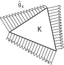
Refer to caption
Figure 1: Local problem (14) on the element K𝐾K with prescribed tractions g^Ksubscript^𝑔𝐾\widehat{g}_{K}.

All technicalities in the construction of g^Ksubscript^𝑔𝐾\widehat{g}_{K} and 𝒒^H|Kεsubscriptsuperscript^𝒒𝜀conditional𝐻𝐾\widehat{\boldsymbol{q}}^{\varepsilon}_{H|K} are given in [19]. It is fruitful to notice that the overall strategy for constructing 𝒒^Hε𝒮subscriptsuperscript^𝒒𝜀𝐻𝒮\widehat{\boldsymbol{q}}^{\varepsilon}_{H}\in\mathcal{S} is particularly suited to the MsFEM framework. Indeed, it is based on fine-scale computations at the macro element level only. These can be performed in the offline stage of MsFEM while constructing the multiscale basis functions.

4 Goal-oriented error estimation

A posteriori error estimation on some outputs of the computation (which are typically needed for decision-making) is often very interesting for engineering applications. In many practical problems, one may indeed be interested in approximating some functional Q(uε)𝑄superscript𝑢𝜀Q(u^{\varepsilon}), referred to as the quantity of interest, rather than the solution uεsuperscript𝑢𝜀u^{\varepsilon} itself. In this section, we address goal-oriented error estimation in the MsFEM framework, again using the CRE concept introduced in Section 3.

4.1 Adjoint problem and classical error indicator

We consider a linear and continuous functional Q:V:𝑄𝑉Q:V\to\mathbb{R}, and assume that our quantity of interest is Q(uε)𝑄superscript𝑢𝜀Q(u^{\varepsilon}). Typical examples include the average of the multiscale solution uεsuperscript𝑢𝜀u^{\varepsilon}, or of the exact flux 𝒒ε=𝔸εuεsuperscript𝒒𝜀superscript𝔸𝜀bold-∇superscript𝑢𝜀\boldsymbol{q}^{\varepsilon}=\mathbb{A}^{\varepsilon}\boldsymbol{\nabla}u^{\varepsilon}, in some region of interest ωQΩsubscript𝜔𝑄Ω\omega_{Q}\subset\Omega. We then introduce the following adjoint problem [7, 29]:

Find u~εV such that, for any vV,Bε(u~ε,v)=Q(v),Find u~εV such that, for any vV,superscript𝐵𝜀superscript~𝑢𝜀𝑣𝑄𝑣\text{Find $\widetilde{u}^{\varepsilon}\in V$ such that, for any $v\in V$,}\quad B^{\varepsilon\ast}(\widetilde{u}^{\varepsilon},v)=Q(v), (15)

where Bε(u,v)superscript𝐵𝜀𝑢𝑣B^{\varepsilon\ast}(u,v) is the formal adjoint of the primal form Bε(u,v)superscript𝐵𝜀𝑢𝑣B^{\varepsilon}(u,v), satisfying Bε(u,v)=Bε(v,u)superscript𝐵𝜀𝑢𝑣superscript𝐵𝜀𝑣𝑢B^{\varepsilon\ast}(u,v)=B^{\varepsilon}(v,u). In the current symmetric case, the forms Bεsuperscript𝐵𝜀B^{\varepsilon} and Bεsuperscript𝐵𝜀B^{\varepsilon\ast} are identical. We also define the adjoint flux 𝒒~ε=𝔸εu~εsuperscript~𝒒𝜀superscript𝔸𝜀bold-∇superscript~𝑢𝜀\widetilde{\boldsymbol{q}}^{\varepsilon}=\mathbb{A}^{\varepsilon}\boldsymbol{\nabla}\widetilde{u}^{\varepsilon} and the space of equilibrated fluxes (with regard to the adjoint problem):

𝒮~={𝒑~(div,Ω);vV,Ω𝒑~v=Q(v)}.~𝒮formulae-sequence~𝒑𝑑𝑖𝑣Ωformulae-sequencefor-all𝑣𝑉subscriptΩ~𝒑bold-∇𝑣𝑄𝑣\widetilde{\mathcal{S}}=\left\{\widetilde{\boldsymbol{p}}\in\mathcal{H}(div,\Omega);\quad\forall v\in V,\quad\int_{\Omega}\widetilde{\boldsymbol{p}}\cdot\boldsymbol{\nabla}v=Q(v)\right\}.
Remark 5

In practice, the functional Q𝑄Q is often defined by

Q(v)=Ω(f~Qv+𝒒~Qv)+ΓNg~Qv,𝑄𝑣subscriptΩsubscript~𝑓𝑄𝑣subscript~𝒒𝑄bold-∇𝑣subscriptsubscriptΓ𝑁subscript~𝑔𝑄𝑣Q(v)=\int_{\Omega}\left(\widetilde{f}_{Q}\,v+\widetilde{\boldsymbol{q}}_{Q}\cdot\boldsymbol{\nabla}v\right)+\int_{\Gamma_{N}}\widetilde{g}_{Q}\,v, (16)

where (f~Q,𝐪~Q,g~Q)subscript~𝑓𝑄subscript~𝐪𝑄subscript~𝑔𝑄\left(\widetilde{f}_{Q},\widetilde{\boldsymbol{q}}_{Q},\widetilde{g}_{Q}\right) is a set of extraction functions which can be mechanically interpreted in the adjoint problem as body, pre-flux and traction loadings, respectively.

Remark 6

To handle some particular cases (such as quantities of interest related to the normal flux on ΓDsubscriptΓ𝐷\Gamma_{D}, which correspond to a functional Q𝑄Q defined on a strict subset of V𝑉V), a more general formulation of the adjoint problem can be found in [29].

Remark 7

Pointwise quantities of interest, such as uε(𝐱0)superscript𝑢𝜀subscript𝐱0u^{\varepsilon}(\boldsymbol{x}_{0}) for some 𝐱0Ωsubscript𝐱0Ω\boldsymbol{x}_{0}\in\Omega, cannot be directly considered in this framework since the solution uε1(Ω)superscript𝑢𝜀superscript1Ωu^{\varepsilon}\in\mathcal{H}^{1}(\Omega) may not be continuous (for d2𝑑2d\geq 2). To circumvent this issue, a regularization technique was introduced in [62] for (monoscale) FEM. We do not consider such pointwise quantities of interest here.

The primal-dual equivalence follows for uεsuperscript𝑢𝜀u^{\varepsilon} solution to the primal problem (2) and u~εsuperscript~𝑢𝜀\widetilde{u}^{\varepsilon} solution to the adjoint problem (15):

Q(uε)=Bε(u~ε,uε)=Bε(uε,u~ε)=F(u~ε).𝑄superscript𝑢𝜀superscript𝐵𝜀superscript~𝑢𝜀superscript𝑢𝜀superscript𝐵𝜀superscript𝑢𝜀superscript~𝑢𝜀𝐹superscript~𝑢𝜀Q(u^{\varepsilon})=B^{\varepsilon\ast}(\widetilde{u}^{\varepsilon},u^{\varepsilon})=B^{\varepsilon}(u^{\varepsilon},\widetilde{u}^{\varepsilon})=F(\widetilde{u}^{\varepsilon}).

Let uHεsubscriptsuperscript𝑢𝜀𝐻u^{\varepsilon}_{H} be the MsFEM approximation of uεsuperscript𝑢𝜀u^{\varepsilon}, and let u^Hεsubscriptsuperscript^𝑢𝜀𝐻\widehat{u}^{\varepsilon}_{H} be a function in V𝑉V close to uHεsubscriptsuperscript𝑢𝜀𝐻u^{\varepsilon}_{H} (if we work with a conforming MsFEM approach, then u^Hε=uHεsubscriptsuperscript^𝑢𝜀𝐻subscriptsuperscript𝑢𝜀𝐻\widehat{u}^{\varepsilon}_{H}=u^{\varepsilon}_{H}). From the adjoint solution u~εsuperscript~𝑢𝜀\widetilde{u}^{\varepsilon}, an exact representation of the MsFEM error on the quantity Q(uε)𝑄superscript𝑢𝜀Q(u^{\varepsilon}) is available:

Q(uε)Q(uHε)=Q(uεu^Hε)+ΔQ=Bε(uεu^Hε,u~ε)+ΔQ=Rε(u~ε)+ΔQ,𝑄superscript𝑢𝜀𝑄subscriptsuperscript𝑢𝜀𝐻𝑄superscript𝑢𝜀subscriptsuperscript^𝑢𝜀𝐻Δ𝑄superscript𝐵𝜀superscript𝑢𝜀subscriptsuperscript^𝑢𝜀𝐻superscript~𝑢𝜀Δ𝑄superscript𝑅𝜀superscript~𝑢𝜀Δ𝑄Q(u^{\varepsilon})-Q(u^{\varepsilon}_{H})=Q(u^{\varepsilon}-\widehat{u}^{\varepsilon}_{H})+\Delta Q=B^{\varepsilon}(u^{\varepsilon}-\widehat{u}^{\varepsilon}_{H},\widetilde{u}^{\varepsilon})+\Delta Q=R^{\varepsilon}(\widetilde{u}^{\varepsilon})+\Delta Q, (17)

with ΔQ=Q(u^HεuHε)Δ𝑄𝑄subscriptsuperscript^𝑢𝜀𝐻subscriptsuperscript𝑢𝜀𝐻\Delta Q=Q(\widehat{u}^{\varepsilon}_{H}-u^{\varepsilon}_{H}), and where Rε(v)=F(v)Bε(u^Hε,v)superscript𝑅𝜀𝑣𝐹𝑣superscript𝐵𝜀subscriptsuperscript^𝑢𝜀𝐻𝑣R^{\varepsilon}(v)=F(v)-B^{\varepsilon}(\widehat{u}^{\varepsilon}_{H},v) is the residual functional associated with u^HεVsubscriptsuperscript^𝑢𝜀𝐻𝑉\widehat{u}^{\varepsilon}_{H}\in V. The representation (17) shows that the adjoint solution u~εsuperscript~𝑢𝜀\widetilde{u}^{\varepsilon}, often termed generalized Green’s function, provides for the sensitivity of the error on Q𝑄Q to the local sources of the MsFEM error in the whole domain ΩΩ\Omega.

A convenient error indicator may be derived from (17) using the dual weighted residual (DWR) method proposed in [6] for FEM and extended to multiscale computations in recent works (see for instance [2, 20]). The DWR method is based on hierarchical a posteriori error analysis. We compute an approximate adjoint solution u~+εsubscriptsuperscript~𝑢𝜀\widetilde{u}^{\varepsilon}_{+} from a hierarchically refined MsFEM space V+εVHεsubscriptsuperscript𝑉𝜀𝐻subscriptsuperscript𝑉𝜀V^{\varepsilon}_{+}\supset V^{\varepsilon}_{H} (higher-order basis functions, refined mesh) and we assume that the error between u~εsuperscript~𝑢𝜀\widetilde{u}^{\varepsilon} and u~+εsubscriptsuperscript~𝑢𝜀\widetilde{u}^{\varepsilon}_{+} is small. We then write

Q(uε)Q(uHε)ΔQ=Rε(u~+ε)+Rε(u~εu~+ε)Rε(u~+ε),𝑄superscript𝑢𝜀𝑄subscriptsuperscript𝑢𝜀𝐻Δ𝑄superscript𝑅𝜀subscriptsuperscript~𝑢𝜀superscript𝑅𝜀superscript~𝑢𝜀subscriptsuperscript~𝑢𝜀superscript𝑅𝜀subscriptsuperscript~𝑢𝜀Q(u^{\varepsilon})-Q(u^{\varepsilon}_{H})-\Delta Q=R^{\varepsilon}(\widetilde{u}^{\varepsilon}_{+})+R^{\varepsilon}(\widetilde{u}^{\varepsilon}-\widetilde{u}^{\varepsilon}_{+})\approx R^{\varepsilon}(\widetilde{u}^{\varepsilon}_{+}), (18)

where the right-hand side and ΔQΔ𝑄\Delta Q are fully computable.

Remark 8

Due to the Galerkin orthogonality, choosing the same MsFEM space VHεsubscriptsuperscript𝑉𝜀𝐻V^{\varepsilon}_{H} to compute uHεsubscriptsuperscript𝑢𝜀𝐻u^{\varepsilon}_{H} and u~+εsubscriptsuperscript~𝑢𝜀\widetilde{u}^{\varepsilon}_{+} would lead to a meaningless indicator (in that case, we would have Rε(u~+ε)=0superscript𝑅𝜀subscriptsuperscript~𝑢𝜀0R^{\varepsilon}(\widetilde{u}^{\varepsilon}_{+})=0). Consequently, a convenient approximation of the adjoint solution should involve a subspace in (VHε)superscriptsubscriptsuperscript𝑉𝜀𝐻perpendicular-to(V^{\varepsilon}_{H})^{\perp}.

The above argument can be somewhat quantified. Let u+εV+εsubscriptsuperscript𝑢𝜀subscriptsuperscript𝑉𝜀u^{\varepsilon}_{+}\in V^{\varepsilon}_{+} be the approximation (in the refined space) of the primal solution. We assume that the saturation assumption |Q(uε)Q(u+ε)|β|Q(uε)Q(u^Hε)|𝑄superscript𝑢𝜀𝑄subscriptsuperscript𝑢𝜀𝛽𝑄superscript𝑢𝜀𝑄subscriptsuperscript^𝑢𝜀𝐻|Q(u^{\varepsilon})-Q(u^{\varepsilon}_{+})|\leq\beta|Q(u^{\varepsilon})-Q(\widehat{u}^{\varepsilon}_{H})| is satisfied for some 0β<10𝛽10\leq\beta<1. Using the fact that u+εu^HεV+εsubscriptsuperscript𝑢𝜀subscriptsuperscript^𝑢𝜀𝐻subscriptsuperscript𝑉𝜀u^{\varepsilon}_{+}-\widehat{u}^{\varepsilon}_{H}\in V^{\varepsilon}_{+} and next the fact that u~+εV+εsubscriptsuperscript~𝑢𝜀subscriptsuperscript𝑉𝜀\widetilde{u}^{\varepsilon}_{+}\in V^{\varepsilon}_{+}, we obtain

Q(u+ε)Q(u^Hε)=Bε(u+εu^Hε,u~+ε)=Bε(uεu^Hε,u~+ε)=Rε(u~+ε).𝑄subscriptsuperscript𝑢𝜀𝑄subscriptsuperscript^𝑢𝜀𝐻superscript𝐵𝜀subscriptsuperscript𝑢𝜀subscriptsuperscript^𝑢𝜀𝐻subscriptsuperscript~𝑢𝜀superscript𝐵𝜀superscript𝑢𝜀subscriptsuperscript^𝑢𝜀𝐻subscriptsuperscript~𝑢𝜀superscript𝑅𝜀subscriptsuperscript~𝑢𝜀Q(u^{\varepsilon}_{+})-Q(\widehat{u}^{\varepsilon}_{H})=B^{\varepsilon}(u^{\varepsilon}_{+}-\widehat{u}^{\varepsilon}_{H},\widetilde{u}^{\varepsilon}_{+})=B^{\varepsilon}(u^{\varepsilon}-\widehat{u}^{\varepsilon}_{H},\widetilde{u}^{\varepsilon}_{+})=R^{\varepsilon}(\widetilde{u}^{\varepsilon}_{+}).

Using the triangle inequality, we get

|Rε(u~+ε)|1+β|Q(uε)Q(uHε)ΔQ||Rε(u~+ε)|1β,superscript𝑅𝜀subscriptsuperscript~𝑢𝜀1𝛽𝑄superscript𝑢𝜀𝑄subscriptsuperscript𝑢𝜀𝐻Δ𝑄superscript𝑅𝜀subscriptsuperscript~𝑢𝜀1𝛽\frac{|R^{\varepsilon}(\widetilde{u}^{\varepsilon}_{+})|}{1+\beta}\leq|Q(u^{\varepsilon})-Q(u^{\varepsilon}_{H})-\Delta Q|\leq\frac{|R^{\varepsilon}(\widetilde{u}^{\varepsilon}_{+})|}{1-\beta},

which quantifies the approximation (18). The indicator defined in (18) may be used to drive adaptive algorithms, but it does not provide for guaranteed error bounds on Q𝑄Q. Alternative techniques are proposed in the next sections.

4.2 Guaranteed error bounds using CRE

In the FEM context, classical approaches to bound the error on a quantity of interest Q𝑄Q consist in solving the primal and adjoint problems with the same approximation space, before using a posteriori bounds available for the error in the energy norm [3]. These approaches can be easily extended to MsFEM with general, conforming or nonconforming, formulations.

Denoting by u~Hεsubscriptsuperscript~𝑢𝜀𝐻\widetilde{u}^{\varepsilon}_{H} the approximate adjoint solution obtained using the space VHεsubscriptsuperscript𝑉𝜀𝐻V^{\varepsilon}_{H}, and potentially post-processing it to define u~^HεVsubscriptsuperscript^~𝑢𝜀𝐻𝑉\widehat{\widetilde{u}}^{\varepsilon}_{H}\in V in case VHεVnot-subset-ofsubscriptsuperscript𝑉𝜀𝐻𝑉V^{\varepsilon}_{H}\not\subset V (see Section 3.1), the equality (17) yields that

Q(uε)Q(uHε)ΔQRε(u~^Hε)=Bε(uεu^Hε,u~εu~^Hε).𝑄superscript𝑢𝜀𝑄subscriptsuperscript𝑢𝜀𝐻Δ𝑄superscript𝑅𝜀subscriptsuperscript^~𝑢𝜀𝐻superscript𝐵𝜀superscript𝑢𝜀subscriptsuperscript^𝑢𝜀𝐻superscript~𝑢𝜀subscriptsuperscript^~𝑢𝜀𝐻Q(u^{\varepsilon})-Q(u^{\varepsilon}_{H})-\Delta Q-R^{\varepsilon}\left(\widehat{\widetilde{u}}^{\varepsilon}_{H}\right)=B^{\varepsilon}\left(u^{\varepsilon}-\widehat{u}^{\varepsilon}_{H},\widetilde{u}^{\varepsilon}-\widehat{\widetilde{u}}^{\varepsilon}_{H}\right). (19)

The Cauchy-Schwarz inequality then yields

|Q(uε)Q(uHε)ΔQRε(u~^Hε)||uεu^Hε||u~εu~^Hε|.𝑄superscript𝑢𝜀𝑄subscriptsuperscript𝑢𝜀𝐻Δ𝑄superscript𝑅𝜀subscriptsuperscript^~𝑢𝜀𝐻normsuperscript𝑢𝜀subscriptsuperscript^𝑢𝜀𝐻normsuperscript~𝑢𝜀subscriptsuperscript^~𝑢𝜀𝐻\left|Q(u^{\varepsilon})-Q(u^{\varepsilon}_{H})-\Delta Q-R^{\varepsilon}\left(\widehat{\widetilde{u}}^{\varepsilon}_{H}\right)\right|\leq{\left|\kern-1.07639pt\left|\kern-1.07639pt\left|u^{\varepsilon}-\widehat{u}^{\varepsilon}_{H}\right|\kern-1.07639pt\right|\kern-1.07639pt\right|}\ {\left|\kern-1.07639pt\left|\kern-1.07639pt\left|\widetilde{u}^{\varepsilon}-\widehat{\widetilde{u}}^{\varepsilon}_{H}\right|\kern-1.07639pt\right|\kern-1.07639pt\right|}. (20)
Remark 9

In the conforming formulation of MsFEM (i.e. when VHεVsubscriptsuperscript𝑉𝜀𝐻𝑉V^{\varepsilon}_{H}\subset V), we can take u^Hε=uHεsubscriptsuperscript^𝑢𝜀𝐻subscriptsuperscript𝑢𝜀𝐻\widehat{u}^{\varepsilon}_{H}=u^{\varepsilon}_{H} and u~^Hε=u~Hεsubscriptsuperscript^~𝑢𝜀𝐻subscriptsuperscript~𝑢𝜀𝐻\widehat{\widetilde{u}}^{\varepsilon}_{H}=\widetilde{u}^{\varepsilon}_{H} so that the Galerkin orthogonality Rε(u~^Hε)=0superscript𝑅𝜀subscriptsuperscript^~𝑢𝜀𝐻0\displaystyle R^{\varepsilon}\left(\widehat{\widetilde{u}}^{\varepsilon}_{H}\right)=0 holds. The result (20) can be recast as

|Q(uε)Q(uHε)||uεuHε||u~εu~Hε|.𝑄superscript𝑢𝜀𝑄subscriptsuperscript𝑢𝜀𝐻normsuperscript𝑢𝜀subscriptsuperscript𝑢𝜀𝐻normsuperscript~𝑢𝜀subscriptsuperscript~𝑢𝜀𝐻|Q(u^{\varepsilon})-Q(u^{\varepsilon}_{H})|\leq{\left|\kern-1.07639pt\left|\kern-1.07639pt\left|u^{\varepsilon}-u^{\varepsilon}_{H}\right|\kern-1.07639pt\right|\kern-1.07639pt\right|}\ {\left|\kern-1.07639pt\left|\kern-1.07639pt\left|\widetilde{u}^{\varepsilon}-\widetilde{u}^{\varepsilon}_{H}\right|\kern-1.07639pt\right|\kern-1.07639pt\right|}.

This is a classical result in the monoscale conforming FEM context.

Consequently, guaranteed error bounds on Q𝑄Q can be obtained from any guaranteed a posteriori global error estimate on |uεu^Hε|normsuperscript𝑢𝜀subscriptsuperscript^𝑢𝜀𝐻{\left|\kern-1.07639pt\left|\kern-1.07639pt\left|u^{\varepsilon}-\widehat{u}^{\varepsilon}_{H}\right|\kern-1.07639pt\right|\kern-1.07639pt\right|} and |u~εu~^Hε|normsuperscript~𝑢𝜀subscriptsuperscript^~𝑢𝜀𝐻{\left|\kern-1.07639pt\left|\kern-1.07639pt\left|\widetilde{u}^{\varepsilon}-\widehat{\widetilde{u}}^{\varepsilon}_{H}\right|\kern-1.07639pt\right|\kern-1.07639pt\right|}. Using the CRE concept introduced in Section 3, (20) yields the a posteriori estimate

|Q(uε)Q(uHε)ΔQRε(u~^Hε)|ECRE(u^Hε,𝒒^Hε)ECRE(u~^Hε,𝒒~^Hε),𝑄superscript𝑢𝜀𝑄subscriptsuperscript𝑢𝜀𝐻Δ𝑄superscript𝑅𝜀subscriptsuperscript^~𝑢𝜀𝐻subscript𝐸𝐶𝑅𝐸subscriptsuperscript^𝑢𝜀𝐻subscriptsuperscript^𝒒𝜀𝐻subscript𝐸𝐶𝑅𝐸subscriptsuperscript^~𝑢𝜀𝐻subscriptsuperscript^~𝒒𝜀𝐻\left|Q(u^{\varepsilon})-Q(u^{\varepsilon}_{H})-\Delta Q-R^{\varepsilon}\left(\widehat{\widetilde{u}}^{\varepsilon}_{H}\right)\right|\leq E_{CRE}(\widehat{u}^{\varepsilon}_{H},\widehat{\boldsymbol{q}}^{\varepsilon}_{H})\,E_{CRE}\left(\widehat{\widetilde{u}}^{\varepsilon}_{H},\widehat{\widetilde{\boldsymbol{q}}}^{\varepsilon}_{H}\right), (21)

where 𝒒^Hε𝒮subscriptsuperscript^𝒒𝜀𝐻𝒮\widehat{\boldsymbol{q}}^{\varepsilon}_{H}\in\mathcal{S}, resp. 𝒒~^Hε𝒮~subscriptsuperscript^~𝒒𝜀𝐻~𝒮\widehat{\widetilde{\boldsymbol{q}}}^{\varepsilon}_{H}\in\widetilde{\mathcal{S}}, is constructed as a post-processing of 𝒒Hεsubscriptsuperscript𝒒𝜀𝐻\boldsymbol{q}^{\varepsilon}_{H}, resp. 𝒒~Hεsubscriptsuperscript~𝒒𝜀𝐻\widetilde{\boldsymbol{q}}^{\varepsilon}_{H}, as detailed in Section 3.2. However, the estimate (21), based on the Cauchy-Schwarz inequality over the whole domain ΩΩ\Omega, does not exploit the locality of Q𝑄Q. It thus leads to crude upper bounds when MsFEM errors for primal and adjoint problems have disjoint supports. A better estimate would consist in using the Cauchy-Schwarz inequality at the element level, under the form

|Q(uε)Q(uHε)ΔQRε(u~^Hε)|K|uεu^Hε||K|u~εu~^Hε||K.\left|Q(u^{\varepsilon})-Q(u^{\varepsilon}_{H})-\Delta Q-R^{\varepsilon}\left(\widehat{\widetilde{u}}^{\varepsilon}_{H}\right)\right|\leq\sum_{K}{\left|\kern-1.07639pt\left|\kern-1.07639pt\left|u^{\varepsilon}-\widehat{u}^{\varepsilon}_{H}\right|\kern-1.07639pt\right|\kern-1.07639pt\right|}_{|K}\ {\left|\kern-1.07639pt\left|\kern-1.07639pt\left|\widetilde{u}^{\varepsilon}-\widehat{\widetilde{u}}^{\varepsilon}_{H}\right|\kern-1.07639pt\right|\kern-1.07639pt\right|}_{|K}.

However, computable upper bounds on the error in the energy norm restricted to each element K𝐾K are hardly available, even though recent works such as [43] have proposed first ideas in that direction.

An alternative and more accurate estimate than (21) can be constructed by taking advantage of the property (10) of the CRE concept. Indeed, we infer from (19) that

Q(uε)Q(uHε)ΔQRε(u~^Hε)𝑄superscript𝑢𝜀𝑄subscriptsuperscript𝑢𝜀𝐻Δ𝑄superscript𝑅𝜀subscriptsuperscript^~𝑢𝜀𝐻\displaystyle Q(u^{\varepsilon})-Q(u^{\varepsilon}_{H})-\Delta Q-R^{\varepsilon}\left(\widehat{\widetilde{u}}^{\varepsilon}_{H}\right) =Bε(uεu^Hε,u~εu~^Hε)absentsuperscript𝐵𝜀superscript𝑢𝜀subscriptsuperscript^𝑢𝜀𝐻superscript~𝑢𝜀subscriptsuperscript^~𝑢𝜀𝐻\displaystyle=B^{\varepsilon}\left(u^{\varepsilon}-\widehat{u}^{\varepsilon}_{H},\widetilde{u}^{\varepsilon}-\widehat{\widetilde{u}}^{\varepsilon}_{H}\right)
=Ω(uεu^Hε)(𝒒~ε𝔸εu~^Hε)absentsubscriptΩbold-∇superscript𝑢𝜀subscriptsuperscript^𝑢𝜀𝐻superscript~𝒒𝜀superscript𝔸𝜀bold-∇subscriptsuperscript^~𝑢𝜀𝐻\displaystyle=\int_{\Omega}\boldsymbol{\nabla}(u^{\varepsilon}-\widehat{u}^{\varepsilon}_{H})\cdot\left(\widetilde{\boldsymbol{q}}^{\varepsilon}-\mathbb{A}^{\varepsilon}\boldsymbol{\nabla}\widehat{\widetilde{u}}^{\varepsilon}_{H}\right)
=Ω(uεu^Hε)(𝒒~^Hε𝔸εu~^Hε)absentsubscriptΩbold-∇superscript𝑢𝜀subscriptsuperscript^𝑢𝜀𝐻superscriptsubscript^~𝒒𝐻𝜀superscript𝔸𝜀bold-∇subscriptsuperscript^~𝑢𝜀𝐻\displaystyle=\int_{\Omega}\boldsymbol{\nabla}(u^{\varepsilon}-\widehat{u}^{\varepsilon}_{H})\cdot\left(\widehat{\widetilde{\boldsymbol{q}}}_{H}^{\varepsilon}-\mathbb{A}^{\varepsilon}\boldsymbol{\nabla}\widehat{\widetilde{u}}^{\varepsilon}_{H}\right)
=Ω(𝔸ε)1(𝒒ε𝒒^Hε)(𝒒~^Hε𝔸εu~^Hε)+CHε,absentsubscriptΩsuperscriptsuperscript𝔸𝜀1superscript𝒒𝜀subscriptsuperscript^𝒒𝜀𝐻superscriptsubscript^~𝒒𝐻𝜀superscript𝔸𝜀bold-∇subscriptsuperscript^~𝑢𝜀𝐻subscriptsuperscript𝐶𝜀𝐻\displaystyle=\int_{\Omega}(\mathbb{A}^{\varepsilon})^{-1}\left(\boldsymbol{q}^{\varepsilon}-\widehat{\boldsymbol{q}}^{\varepsilon\ast}_{H}\right)\cdot\left(\widehat{\widetilde{\boldsymbol{q}}}_{H}^{\varepsilon}-\mathbb{A}^{\varepsilon}\boldsymbol{\nabla}\widehat{\widetilde{u}}^{\varepsilon}_{H}\right)+C^{\varepsilon}_{H}, (22)

with 𝒒^Hε=(𝒒^Hε+𝔸εu^Hε)/2subscriptsuperscript^𝒒𝜀𝐻subscriptsuperscript^𝒒𝜀𝐻superscript𝔸𝜀bold-∇subscriptsuperscript^𝑢𝜀𝐻2\widehat{\boldsymbol{q}}^{\varepsilon\ast}_{H}=(\widehat{\boldsymbol{q}}^{\varepsilon}_{H}+\mathbb{A}^{\varepsilon}\boldsymbol{\nabla}\widehat{u}^{\varepsilon}_{H})/2 and CHεsubscriptsuperscript𝐶𝜀𝐻C^{\varepsilon}_{H} a computable term defined by

CHε=Ω(𝔸ε)1(𝒒^Hε𝔸εu^Hε)(𝒒~^Hε𝔸εu~^Hε)=12Ω(𝔸ε)1(𝒒^Hε𝔸εu^Hε)(𝒒~^Hε𝔸εu~^Hε).subscriptsuperscript𝐶𝜀𝐻subscriptΩsuperscriptsuperscript𝔸𝜀1subscriptsuperscript^𝒒𝜀𝐻superscript𝔸𝜀bold-∇subscriptsuperscript^𝑢𝜀𝐻superscriptsubscript^~𝒒𝐻𝜀superscript𝔸𝜀bold-∇subscriptsuperscript^~𝑢𝜀𝐻12subscriptΩsuperscriptsuperscript𝔸𝜀1subscriptsuperscript^𝒒𝜀𝐻superscript𝔸𝜀bold-∇subscriptsuperscript^𝑢𝜀𝐻superscriptsubscript^~𝒒𝐻𝜀superscript𝔸𝜀bold-∇subscriptsuperscript^~𝑢𝜀𝐻C^{\varepsilon}_{H}=\int_{\Omega}(\mathbb{A}^{\varepsilon})^{-1}\left(\widehat{\boldsymbol{q}}^{\varepsilon\ast}_{H}-\mathbb{A}^{\varepsilon}\boldsymbol{\nabla}\widehat{u}^{\varepsilon}_{H}\right)\cdot\left(\widehat{\widetilde{\boldsymbol{q}}}_{H}^{\varepsilon}-\mathbb{A}^{\varepsilon}\boldsymbol{\nabla}\widehat{\widetilde{u}}^{\varepsilon}_{H}\right)=\frac{1}{2}\int_{\Omega}(\mathbb{A}^{\varepsilon})^{-1}\left(\widehat{\boldsymbol{q}}^{\varepsilon}_{H}-\mathbb{A}^{\varepsilon}\boldsymbol{\nabla}\widehat{u}^{\varepsilon}_{H}\right)\cdot\left(\widehat{\widetilde{\boldsymbol{q}}}_{H}^{\varepsilon}-\mathbb{A}^{\varepsilon}\boldsymbol{\nabla}\widehat{\widetilde{u}}^{\varepsilon}_{H}\right).

We next get from (22) that

Q(uε)Q(uHε)ΔQC¯Hε=Ω(𝔸ε)1(𝒒ε𝒒^Hε)(𝒒~^Hε𝔸εu~^Hε)𝑄superscript𝑢𝜀𝑄subscriptsuperscript𝑢𝜀𝐻Δ𝑄subscriptsuperscript¯𝐶𝜀𝐻subscriptΩsuperscriptsuperscript𝔸𝜀1superscript𝒒𝜀subscriptsuperscript^𝒒𝜀𝐻superscriptsubscript^~𝒒𝐻𝜀superscript𝔸𝜀bold-∇subscriptsuperscript^~𝑢𝜀𝐻Q(u^{\varepsilon})-Q(u^{\varepsilon}_{H})-\Delta Q-\overline{C}^{\varepsilon}_{H}=\int_{\Omega}(\mathbb{A}^{\varepsilon})^{-1}\left(\boldsymbol{q}^{\varepsilon}-\widehat{\boldsymbol{q}}^{\varepsilon\ast}_{H}\right)\cdot\left(\widehat{\widetilde{\boldsymbol{q}}}_{H}^{\varepsilon}-\mathbb{A}^{\varepsilon}\boldsymbol{\nabla}\widehat{\widetilde{u}}^{\varepsilon}_{H}\right)

with

C¯Hε=CHε+Rε(u~^Hε)=12Ω(𝔸ε)1(𝒒^Hε𝔸εu^Hε)(𝒒~^Hε+𝔸εu~^Hε).subscriptsuperscript¯𝐶𝜀𝐻subscriptsuperscript𝐶𝜀𝐻superscript𝑅𝜀subscriptsuperscript^~𝑢𝜀𝐻12subscriptΩsuperscriptsuperscript𝔸𝜀1subscriptsuperscript^𝒒𝜀𝐻superscript𝔸𝜀bold-∇subscriptsuperscript^𝑢𝜀𝐻superscriptsubscript^~𝒒𝐻𝜀superscript𝔸𝜀bold-∇subscriptsuperscript^~𝑢𝜀𝐻\overline{C}^{\varepsilon}_{H}=C^{\varepsilon}_{H}+R^{\varepsilon}\left(\widehat{\widetilde{u}}^{\varepsilon}_{H}\right)=\frac{1}{2}\int_{\Omega}(\mathbb{A}^{\varepsilon})^{-1}\left(\widehat{\boldsymbol{q}}^{\varepsilon}_{H}-\mathbb{A}^{\varepsilon}\boldsymbol{\nabla}\widehat{u}^{\varepsilon}_{H}\right)\cdot\left(\widehat{\widetilde{\boldsymbol{q}}}_{H}^{\varepsilon}+\mathbb{A}^{\varepsilon}\boldsymbol{\nabla}\widehat{\widetilde{u}}^{\varepsilon}_{H}\right).

Using the Cauchy-Schwarz inequality and next (10), we obtain that

|Q(uε)Q(uHε)ΔQC¯Hε||𝒒ε𝒒^Hε||𝒒~^Hε𝔸εu~^Hε|=12ECRE(u^Hε,𝒒^Hε)ECRE(u~^Hε,𝒒~^Hε).𝑄superscript𝑢𝜀𝑄subscriptsuperscript𝑢𝜀𝐻Δ𝑄subscriptsuperscript¯𝐶𝜀𝐻subscriptnormsuperscript𝒒𝜀subscriptsuperscript^𝒒𝜀𝐻subscriptnormsuperscriptsubscript^~𝒒𝐻𝜀superscript𝔸𝜀bold-∇subscriptsuperscript^~𝑢𝜀𝐻12subscript𝐸𝐶𝑅𝐸subscriptsuperscript^𝑢𝜀𝐻subscriptsuperscript^𝒒𝜀𝐻subscript𝐸𝐶𝑅𝐸subscriptsuperscript^~𝑢𝜀𝐻subscriptsuperscript^~𝒒𝜀𝐻\left|Q(u^{\varepsilon})-Q(u^{\varepsilon}_{H})-\Delta Q-\overline{C}^{\varepsilon}_{H}\right|\leq{\left|\kern-1.07639pt\left|\kern-1.07639pt\left|\boldsymbol{q}^{\varepsilon}-\widehat{\boldsymbol{q}}^{\varepsilon\ast}_{H}\right|\kern-1.07639pt\right|\kern-1.07639pt\right|}_{\mathcal{F}}\ {\left|\kern-1.07639pt\left|\kern-1.07639pt\left|\widehat{\widetilde{\boldsymbol{q}}}_{H}^{\varepsilon}-\mathbb{A}^{\varepsilon}\boldsymbol{\nabla}\widehat{\widetilde{u}}^{\varepsilon}_{H}\right|\kern-1.07639pt\right|\kern-1.07639pt\right|}_{\mathcal{F}}=\frac{1}{2}E_{CRE}\left(\widehat{u}^{\varepsilon}_{H},\widehat{\boldsymbol{q}}^{\varepsilon}_{H}\right)\,E_{CRE}\left(\widehat{\widetilde{u}}^{\varepsilon}_{H},\widehat{\widetilde{\boldsymbol{q}}}^{\varepsilon}_{H}\right). (23)

Note that, thanks to the factor 1/2121/2 on the right-hand side, the estimate (23) yields a more accurate estimation of Q(uε)Q(uHε)𝑄superscript𝑢𝜀𝑄subscriptsuperscript𝑢𝜀𝐻Q(u^{\varepsilon})-Q(u^{\varepsilon}_{H}) than (21).

The fully computable quantity Q(uHε)+ΔQ+C¯Hε𝑄subscriptsuperscript𝑢𝜀𝐻Δ𝑄subscriptsuperscript¯𝐶𝜀𝐻Q(u^{\varepsilon}_{H})+\Delta Q+\overline{C}^{\varepsilon}_{H} can be interpreted as a corrected approximation of Q(uε)𝑄superscript𝑢𝜀Q(u^{\varepsilon}). Furthermore, the estimate (23) can also be written as

Q(uε)Q(uHε)=ΔQ+C¯Hε+ζfor some ζ[12ECREE~CRE,12ECREE~CRE],𝑄superscript𝑢𝜀𝑄subscriptsuperscript𝑢𝜀𝐻Δ𝑄subscriptsuperscript¯𝐶𝜀𝐻𝜁for some ζ[12ECREE~CRE,12ECREE~CRE]Q(u^{\varepsilon})-Q(u^{\varepsilon}_{H})=\Delta Q+\overline{C}^{\varepsilon}_{H}+\zeta\quad\text{for some $\zeta\in\left[-\frac{1}{2}E_{CRE}\,\widetilde{E}_{CRE},\frac{1}{2}E_{CRE}\,\widetilde{E}_{CRE}\right]$},

hence

|Q(uε)Q(uHε)|ηQ:=maxθ=±1|ΔQ+C¯Hε+θ2ECREE~CRE|.𝑄superscript𝑢𝜀𝑄subscriptsuperscript𝑢𝜀𝐻superscript𝜂𝑄assignsubscript𝜃plus-or-minus1Δ𝑄subscriptsuperscript¯𝐶𝜀𝐻𝜃2subscript𝐸𝐶𝑅𝐸subscript~𝐸𝐶𝑅𝐸|Q(u^{\varepsilon})-Q(u^{\varepsilon}_{H})|\leq\eta^{Q}:=\max_{\theta=\pm 1}\left|\Delta Q+\overline{C}^{\varepsilon}_{H}+\frac{\theta}{2}E_{CRE}\,\widetilde{E}_{CRE}\right|. (24)

In contrast to (21), the quantity ηQsuperscript𝜂𝑄\eta^{Q} partially takes into account error cancellations.

It is fruitful to notice that the bounds (21) and (23), constructed from the CRE concept, hold for independent (MsFEM) discretizations of the primal and adjoint problems as they are merely based on equilibrium properties. In the following section, we show how a convenient local enrichment of the adjoint approximate solution can thus be advantageously used to get sharp error bounds from (23).

4.3 Non-intrusive local enrichment of the adjoint solution

We extend to the MsFEM context an enrichment technique initially introduced in [30, 17, 39] for goal-oriented error estimation in FEM models. The general idea is to improve the accuracy of the approximate adjoint solution u~Hεsubscriptsuperscript~𝑢𝜀𝐻\widetilde{u}^{\varepsilon}_{H} (or u~^Hεsubscriptsuperscript^~𝑢𝜀𝐻\widehat{\widetilde{u}}^{\varepsilon}_{H}) by adding a priori information on the problem, i.e. given functions whose purpose is to reproduce localized high-gradient components of u~εsuperscript~𝑢𝜀\widetilde{u}^{\varepsilon} (which are difficult to numerically capture) in the vicinity of the adjoint loading region. These functions, referred to as handbook functions and denoted u~handεsubscriptsuperscript~𝑢𝜀𝑎𝑛𝑑\widetilde{u}^{\varepsilon}_{hand} (with associated flux 𝒒~handε=𝔸εu~handεsubscriptsuperscript~𝒒𝜀𝑎𝑛𝑑superscript𝔸𝜀bold-∇subscriptsuperscript~𝑢𝜀𝑎𝑛𝑑\widetilde{\boldsymbol{q}}^{\varepsilon}_{hand}=\mathbb{A}^{\varepsilon}\boldsymbol{\nabla}\widetilde{u}^{\varepsilon}_{hand}), correspond to generalized Green’s functions. In analogy to (15), they satisfy

Find u~handε01(Ωhand) such that, for any v01(Ωhand),Bε(u~handε,v)=Qhand(v),Find u~handε01(Ωhand) such that, for any v01(Ωhand),superscript𝐵𝜀subscriptsuperscript~𝑢𝜀𝑎𝑛𝑑𝑣subscript𝑄𝑎𝑛𝑑𝑣\text{Find $\widetilde{u}^{\varepsilon}_{hand}\in\mathcal{H}^{1}_{0}(\Omega_{hand})$ such that, for any $v\in\mathcal{H}^{1}_{0}(\Omega_{hand})$,}\quad B^{\varepsilon\ast}(\widetilde{u}^{\varepsilon}_{hand},v)=Q_{hand}(v), (25)

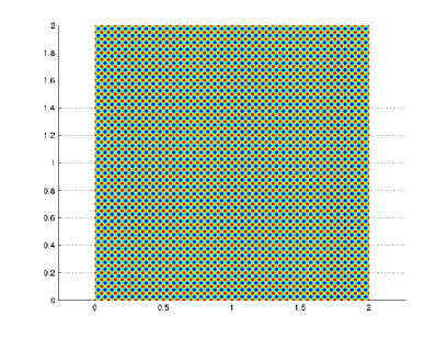
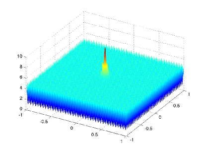
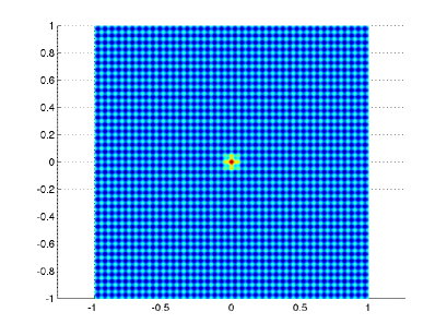
where Qhandsubscript𝑄𝑎𝑛𝑑Q_{hand} is an auxiliary quantity of interest (the eventual quantity of interest Q𝑄Q in (15) may be equal to Qhandsubscript𝑄𝑎𝑛𝑑Q_{hand}, or a linear combination of various Qhandsubscript𝑄𝑎𝑛𝑑Q_{hand}, or various translations of Qhandsubscript𝑄𝑎𝑛𝑑Q_{hand}, …). The domain ΩhandΩsubscriptΩ𝑎𝑛𝑑Ω\Omega_{hand}\subset\Omega is chosen to be sufficiently large, so that the solution to the above problem with 01(Ωhand)subscriptsuperscript10subscriptΩ𝑎𝑛𝑑\mathcal{H}^{1}_{0}(\Omega_{hand}) replaced by V𝑉V would indeed be close to zero on ΩhandsubscriptΩ𝑎𝑛𝑑\partial\Omega_{hand}. In practice, u~handεsubscriptsuperscript~𝑢𝜀𝑎𝑛𝑑\widetilde{u}^{\varepsilon}_{hand} is numerically pre-computed, using an accurate fine scale discretization. Examples of such enrichment functions, for a 2D multiscale medium described by 𝔸ε=Aε𝕀2superscript𝔸𝜀superscript𝐴𝜀subscript𝕀2\mathbb{A}^{\varepsilon}=A^{\varepsilon}\,\mathbb{I}_{2} with Aε(x1,x2)=3+cos(2πx1/ε)+cos(2πx2/ε)superscript𝐴𝜀subscript𝑥1subscript𝑥232𝜋subscript𝑥1𝜀2𝜋subscript𝑥2𝜀A^{\varepsilon}(x_{1},x_{2})=3+\cos(2\pi x_{1}/\varepsilon)+\cos(2\pi x_{2}/\varepsilon) and ε=1/20𝜀120\varepsilon=1/20 (see Fig. 2), are given below.

Refer to caption
Figure 2: Evolution of the material parameter.

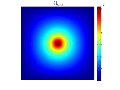
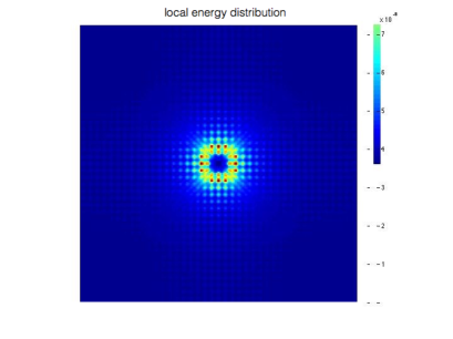
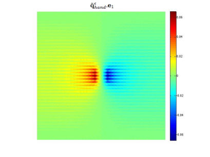
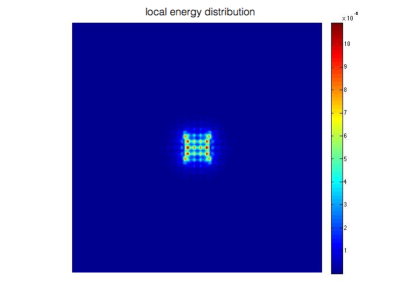
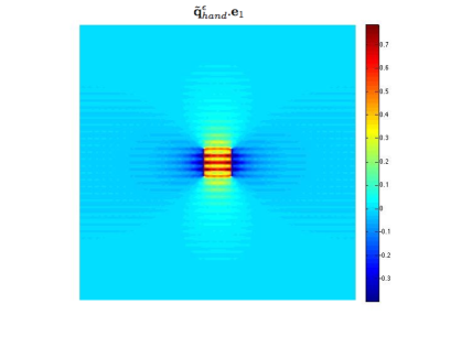
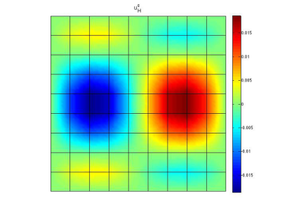
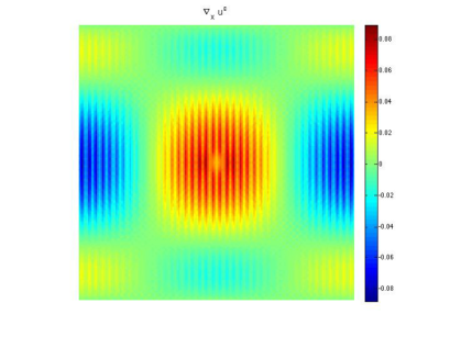
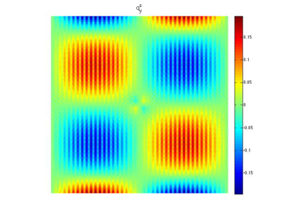
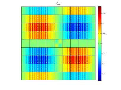
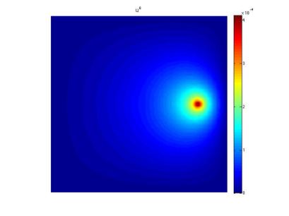
A first example corresponds to a linear functional Q𝑄Q given by (16) with 𝒒~Q=0subscript~𝒒𝑄0\widetilde{\boldsymbol{q}}_{Q}=0, g~Q=0subscript~𝑔𝑄0\widetilde{g}_{Q}=0 and a localized body force f~Q=0subscript~𝑓𝑄0\widetilde{f}_{Q}=0 except in the square domain ωQsubscript𝜔𝑄\omega_{Q}, centered at the center of ΩΩ\Omega and of size 4ε×4ε4𝜀4𝜀4\varepsilon\times 4\varepsilon, where f~Q=1subscript~𝑓𝑄1\widetilde{f}_{Q}=1. Such a quantity of interest corresponds to the average of uεsuperscript𝑢𝜀u^{\varepsilon} in ωQsubscript𝜔𝑄\omega_{Q}. The corresponding handbook function is shown in Fig. 3.

Remark 10

Here and in all what follows, the quantity of interest is given by (16) for some f~Qsubscript~𝑓𝑄\widetilde{f}_{Q} and 𝐪~Qsubscript~𝐪𝑄\widetilde{\boldsymbol{q}}_{Q}, with g~Q=0subscript~𝑔𝑄0\widetilde{g}_{Q}=0. We take for ΩhandsubscriptΩ𝑎𝑛𝑑\Omega_{hand} a domain 10 times as large (in each direction) as the support of f~Qsubscript~𝑓𝑄\widetilde{f}_{Q} and 𝐪~Qsubscript~𝐪𝑄\widetilde{\boldsymbol{q}}_{Q}. For the example discussed above, we thus choose for ΩhandsubscriptΩ𝑎𝑛𝑑\Omega_{hand} a square domain centered at the center of ΩΩ\Omega and of size 40ε×40ε40𝜀40𝜀40\varepsilon\times 40\varepsilon.

Refer to caption
Refer to caption
Refer to caption
Refer to caption
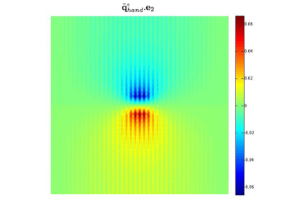
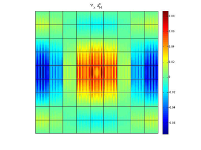
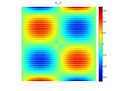
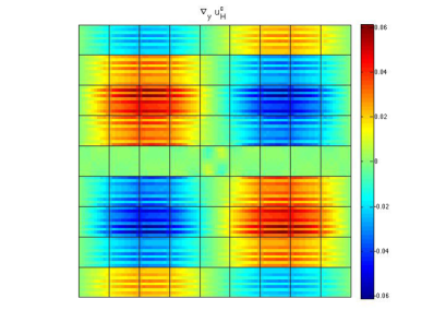
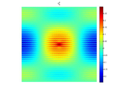
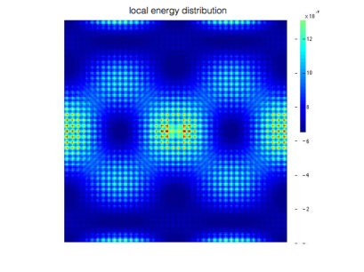
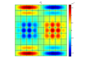
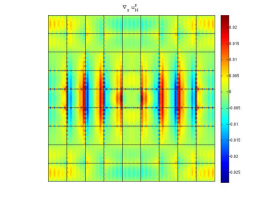
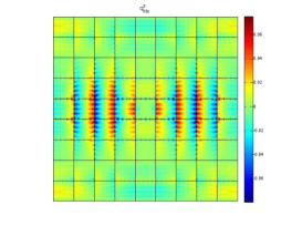
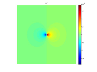
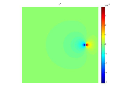
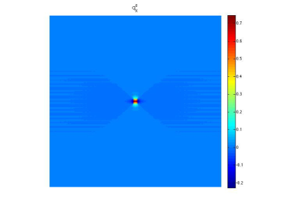
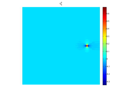
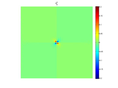
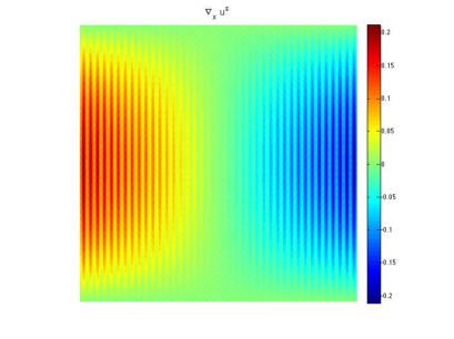
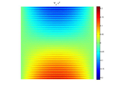
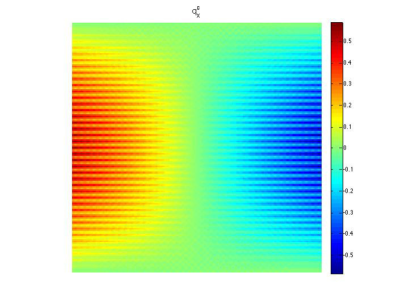
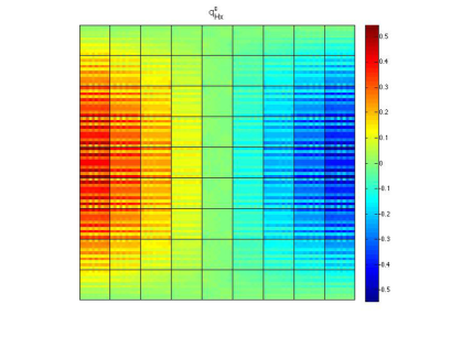
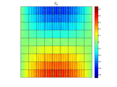
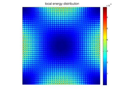
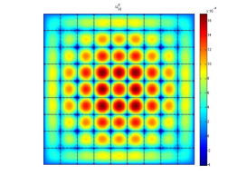
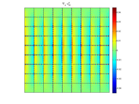
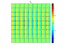
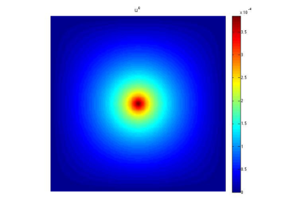
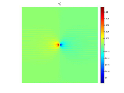
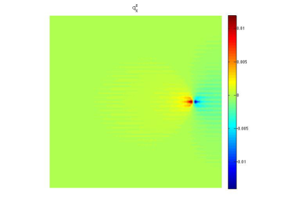
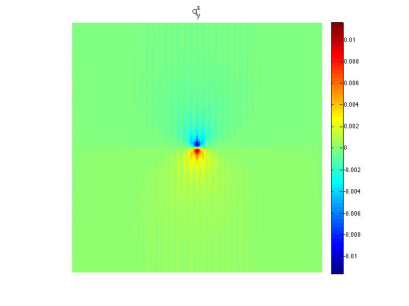
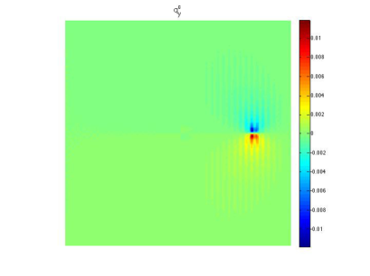
Figure 3: Handbook function in a sufficiently large domain subjected to a constant body force in a local square region ωQsubscript𝜔𝑄\omega_{Q}: u~handεsubscriptsuperscript~𝑢𝜀𝑎𝑛𝑑\widetilde{u}^{\varepsilon}_{hand} (top left), energy distribution (top right), 𝒒~handε𝒆1subscriptsuperscript~𝒒𝜀𝑎𝑛𝑑subscript𝒆1\widetilde{\boldsymbol{q}}^{\varepsilon}_{hand}\cdot\boldsymbol{e}_{1} (bottom left) and 𝒒~handε𝒆2subscriptsuperscript~𝒒𝜀𝑎𝑛𝑑subscript𝒆2\widetilde{\boldsymbol{q}}^{\varepsilon}_{hand}\cdot\boldsymbol{e}_{2} (bottom right).

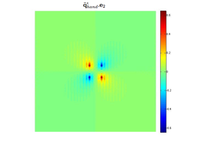
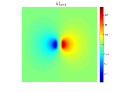
A second example corresponds to a linear functional Q𝑄Q given by (16) with f~Q=0subscript~𝑓𝑄0\widetilde{f}_{Q}=0, g~Q=0subscript~𝑔𝑄0\widetilde{g}_{Q}=0 and a localized pre-flux 𝒒~Q=(1,0)Tsubscript~𝒒𝑄superscript1.0𝑇\widetilde{\boldsymbol{q}}_{Q}=(1,0)^{T} in the same domain ωQsubscript𝜔𝑄\omega_{Q} as above, and 𝒒~Q=0subscript~𝒒𝑄0\widetilde{\boldsymbol{q}}_{Q}=0 elsewhere in ΩΩ\Omega. Such a quantity of interest corresponds to the average of 𝒆1uεsubscript𝒆1superscript𝑢𝜀\boldsymbol{e}_{1}\cdot\nabla u^{\varepsilon} in ωQsubscript𝜔𝑄\omega_{Q}. The corresponding handbook function is shown in Fig. 4.
Refer to caption
Refer to caption
Refer to caption
Refer to caption
Figure 4: Handbook function in a sufficiently large domain subjected to a constant pre-flux in a local square region ωQsubscript𝜔𝑄\omega_{Q}: u~handεsubscriptsuperscript~𝑢𝜀𝑎𝑛𝑑\widetilde{u}^{\varepsilon}_{hand} (top left), energy distribution (top right), 𝒒~handε𝒆1subscriptsuperscript~𝒒𝜀𝑎𝑛𝑑subscript𝒆1\widetilde{\boldsymbol{q}}^{\varepsilon}_{hand}\cdot\boldsymbol{e}_{1} (bottom left) and 𝒒~handε𝒆2subscriptsuperscript~𝒒𝜀𝑎𝑛𝑑subscript𝒆2\widetilde{\boldsymbol{q}}^{\varepsilon}_{hand}\cdot\boldsymbol{e}_{2} (bottom right).

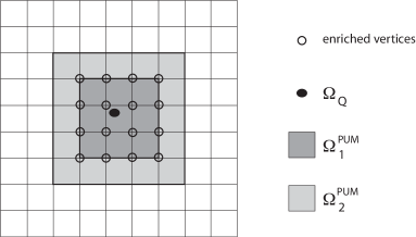
Handbook functions are then locally and seamlessly inserted in the overall procedure, as we explain now. Let ΩQsubscriptΩ𝑄\Omega_{Q} be the area of interest over which the quantity Q𝑄Q is defined, i.e. the region which supports the extraction functions f~Qsubscript~𝑓𝑄\widetilde{f}_{Q} and 𝒒~Qsubscript~𝒒𝑄\widetilde{\boldsymbol{q}}_{Q} (recall (16) and Remark 10). We next introduce some domain Ω1PUMΩhandsuperscriptsubscriptΩ1𝑃𝑈𝑀subscriptΩ𝑎𝑛𝑑\Omega_{1}^{PUM}\subset\Omega_{hand}, which is the union of some coarse elements of 𝒯Hsubscript𝒯𝐻\mathcal{T}_{H}, and which contains ΩQsubscriptΩ𝑄\Omega_{Q} (see Fig. 5). Its boundary is denoted Ω1PUMsuperscriptsubscriptΩ1𝑃𝑈𝑀\partial\Omega_{1}^{PUM}. Let PUMsuperscript𝑃𝑈𝑀\mathcal{I}^{PUM} be the subset of vertices in 𝒯Hsubscript𝒯𝐻\mathcal{T}_{H} which are located in Ω1PUM¯¯superscriptsubscriptΩ1𝑃𝑈𝑀\overline{\Omega_{1}^{PUM}}, so that

Ω1PUM={𝒙Ω;iPUMϕi0(𝒙)=1}.superscriptsubscriptΩ1𝑃𝑈𝑀formulae-sequence𝒙Ωsubscript𝑖superscript𝑃𝑈𝑀subscriptsuperscriptitalic-ϕ0𝑖𝒙1\Omega_{1}^{PUM}=\left\{\boldsymbol{x}\in\Omega;\quad\sum_{i\in\mathcal{I}^{PUM}}\phi^{0}_{i}(\boldsymbol{x})=1\right\}.

We next introduce

Ω2PUM={𝒙Ω;iPUMϕi0(𝒙)(0,1)}superscriptsubscriptΩ2𝑃𝑈𝑀formulae-sequence𝒙Ωsubscript𝑖superscript𝑃𝑈𝑀subscriptsuperscriptitalic-ϕ0𝑖𝒙0.1\Omega_{2}^{PUM}=\left\{\boldsymbol{x}\in\Omega;\quad\sum_{i\in\mathcal{I}^{PUM}}\phi^{0}_{i}(\boldsymbol{x})\in(0,1)\right\}

and see that Ω1PUMΩ2PUM=Supp(iPUMϕi0)ΩsuperscriptsubscriptΩ1𝑃𝑈𝑀superscriptsubscriptΩ2𝑃𝑈𝑀Suppsubscript𝑖superscript𝑃𝑈𝑀subscriptsuperscriptitalic-ϕ0𝑖Ω\displaystyle\Omega_{1}^{PUM}\cup\Omega_{2}^{PUM}=\text{Supp}\left(\sum_{i\in\mathcal{I}^{PUM}}\phi^{0}_{i}\right)\subset\Omega.

Remark 11

In the numerical examples of Section 6.1, ΩQsubscriptΩ𝑄\Omega_{Q} is a square of size 4ε×4ε4𝜀4𝜀4\varepsilon\times 4\varepsilon, and we take for Ω1PUMsuperscriptsubscriptΩ1𝑃𝑈𝑀\Omega_{1}^{PUM} the coarse element containing ΩQsubscriptΩ𝑄\Omega_{Q}. In the numerical example of Section 6.2, ΩQsubscriptΩ𝑄\Omega_{Q} is a square of size 0.1×0.101010.1\times 0.1, and the initial coarse meshsize is H=0.1𝐻01H=0.1. We then take for Ω1PUMsuperscriptsubscriptΩ1𝑃𝑈𝑀\Omega_{1}^{PUM} the union of the coarse element equal to ΩQsubscriptΩ𝑄\Omega_{Q} and of the 8 coarse elements surrounding it.
Refer to caption
Figure 5: Definition of Ω1PUMsuperscriptsubscriptΩ1𝑃𝑈𝑀\Omega_{1}^{PUM} and Ω2PUMsuperscriptsubscriptΩ2𝑃𝑈𝑀\Omega_{2}^{PUM}, for a given ΩQsubscriptΩ𝑄\Omega_{Q}.

The enrichment approach consists in approximating the adjoint solution u~εsuperscript~𝑢𝜀\widetilde{u}^{\varepsilon} by

u~+ε=u~handεiPUMϕi0+u~res,Hε,subscriptsuperscript~𝑢𝜀subscriptsuperscript~𝑢𝜀𝑎𝑛𝑑subscript𝑖superscript𝑃𝑈𝑀subscriptsuperscriptitalic-ϕ0𝑖subscriptsuperscript~𝑢𝜀𝑟𝑒𝑠𝐻\widetilde{u}^{\varepsilon}_{+}=\widetilde{u}^{\varepsilon}_{hand}\sum_{i\in\mathcal{I}^{PUM}}\phi^{0}_{i}+\widetilde{u}^{\varepsilon}_{res,H}, (26)

where u~res,Hεsubscriptsuperscript~𝑢𝜀𝑟𝑒𝑠𝐻\widetilde{u}^{\varepsilon}_{res,H} is an approximate residual solution which is computed using the MsFEM approximation space VHεsubscriptsuperscript𝑉𝜀𝐻V^{\varepsilon}_{H}. We emphasize that

  • 1.

    no additional degree of freedom is associated with the enrichment part, in contrast to other similar enrichment methods such as XFEM or GFEM (where the approximation would read iPUMαiϕi0u~handε+u~res,Hεsubscript𝑖superscript𝑃𝑈𝑀subscript𝛼𝑖subscriptsuperscriptitalic-ϕ0𝑖subscriptsuperscript~𝑢𝜀𝑎𝑛𝑑subscriptsuperscript~𝑢𝜀𝑟𝑒𝑠𝐻\displaystyle\sum_{i\in\mathcal{I}^{PUM}}\alpha_{i}\,\phi^{0}_{i}\,\widetilde{u}^{\varepsilon}_{hand}+\widetilde{u}^{\varepsilon}_{res,H} for some additional unknown coefficients αisubscript𝛼𝑖\alpha_{i} and with u~res,HεVHεsubscriptsuperscript~𝑢𝜀𝑟𝑒𝑠𝐻subscriptsuperscript𝑉𝜀𝐻\widetilde{u}^{\varepsilon}_{res,H}\in V^{\varepsilon}_{H}). This is due to the fact that u~handεsubscriptsuperscript~𝑢𝜀𝑎𝑛𝑑\widetilde{u}^{\varepsilon}_{hand} aims at representing the local high-gradients due to the singular adjoint loading, which can be fully assessed a priori;

  • 2.

    the strategy uses the same MsFEM discretization space VHεsubscriptsuperscript𝑉𝜀𝐻V^{\varepsilon}_{H} to approximate both the primal and the adjoint problems, even though a higher level of approximation is obtained for the adjoint solution due to the enrichment term. Consequently, all the numerical technicalities (mesh connectivities, stiffness matrix, …) implemented to solve the primal problem can be directly reused to solve the adjoint problem. Only the loadings need to be changed. For this reason, the strategy is called non-intrusive. It fully makes sense in the MsFEM framework where the discretization space is obtained from costly computations performed only once in the offline stage.

Remark 12

The above enrichment methodology can also be used to address goal-oriented error estimation on pointwise quantities of interest (when these are defined), as shown in [17, 39]. In this case, handbook functions correspond to classical Green’s functions. They can be analytically computed for homogeneous and isotropic media.

Remark 13

We have chosen the notations Ω1PUMsuperscriptsubscriptΩ1𝑃𝑈𝑀\Omega_{1}^{PUM}, Ω2PUMsuperscriptsubscriptΩ2𝑃𝑈𝑀\Omega_{2}^{PUM} and PUMsuperscript𝑃𝑈𝑀\mathcal{I}^{PUM} in analogy to those introduced in the XFEM and the GFEM approaches. However, here, no partition of unity property is used.

In view of (15) and (26), and assuming that QhandQsubscript𝑄𝑎𝑛𝑑𝑄Q_{hand}\equiv Q in (25), the problem to be solved numerically consists in finding u~res,HεVHεsubscriptsuperscript~𝑢𝜀𝑟𝑒𝑠𝐻subscriptsuperscript𝑉𝜀𝐻\widetilde{u}^{\varepsilon}_{res,H}\in V^{\varepsilon}_{H} such that

vVHε,Bε(u~res,Hε,v)for-all𝑣subscriptsuperscript𝑉𝜀𝐻superscript𝐵𝜀subscriptsuperscript~𝑢𝜀𝑟𝑒𝑠𝐻𝑣\displaystyle\forall v\in V^{\varepsilon}_{H},\quad B^{\varepsilon\ast}(\widetilde{u}^{\varepsilon}_{res,H},v) =Q(v)Bε(u~handεiPUMϕi0,v)absent𝑄𝑣superscript𝐵𝜀subscriptsuperscript~𝑢𝜀𝑎𝑛𝑑subscript𝑖superscript𝑃𝑈𝑀subscriptsuperscriptitalic-ϕ0𝑖𝑣\displaystyle=Q(v)-B^{\varepsilon\ast}\left(\widetilde{u}^{\varepsilon}_{hand}\sum_{i\in\mathcal{I}^{PUM}}\phi^{0}_{i},v\right)
=Q(v)Ω1PUM𝔸εu~handεvΩ2PUM𝔸ε(u~handεiPUMϕi0)vabsent𝑄𝑣subscriptsuperscriptsubscriptΩ1𝑃𝑈𝑀superscript𝔸𝜀bold-∇subscriptsuperscript~𝑢𝜀𝑎𝑛𝑑bold-∇𝑣subscriptsuperscriptsubscriptΩ2𝑃𝑈𝑀superscript𝔸𝜀bold-∇subscriptsuperscript~𝑢𝜀𝑎𝑛𝑑subscript𝑖superscript𝑃𝑈𝑀subscriptsuperscriptitalic-ϕ0𝑖bold-∇𝑣\displaystyle=Q(v)-\int_{\Omega_{1}^{PUM}}\mathbb{A}^{\varepsilon}\boldsymbol{\nabla}\widetilde{u}^{\varepsilon}_{hand}\cdot\boldsymbol{\nabla}v-\int_{\Omega_{2}^{PUM}}\mathbb{A}^{\varepsilon}\boldsymbol{\nabla}\left(\widetilde{u}^{\varepsilon}_{hand}\sum_{i\in\mathcal{I}^{PUM}}\phi^{0}_{i}\right)\cdot\boldsymbol{\nabla}v
=Ω1PUM(𝔸εu~handε𝒏12)vΩ2PUM𝔸ε(u~handεiPUMϕi0)v,absentsubscriptsuperscriptsubscriptΩ1𝑃𝑈𝑀superscript𝔸𝜀bold-∇subscriptsuperscript~𝑢𝜀𝑎𝑛𝑑subscript𝒏12𝑣subscriptsuperscriptsubscriptΩ2𝑃𝑈𝑀superscript𝔸𝜀bold-∇subscriptsuperscript~𝑢𝜀𝑎𝑛𝑑subscript𝑖superscript𝑃𝑈𝑀subscriptsuperscriptitalic-ϕ0𝑖bold-∇𝑣\displaystyle=-\int_{\partial\Omega_{1}^{PUM}}\left(\mathbb{A}^{\varepsilon}\boldsymbol{\nabla}\widetilde{u}^{\varepsilon}_{hand}\cdot\boldsymbol{n}_{12}\right)v-\int_{\Omega_{2}^{PUM}}\mathbb{A}^{\varepsilon}\boldsymbol{\nabla}\left(\widetilde{u}^{\varepsilon}_{hand}\sum_{i\in\mathcal{I}^{PUM}}\phi^{0}_{i}\right)\cdot\boldsymbol{\nabla}v,

with 𝒏12subscript𝒏12\boldsymbol{n}_{12} is the outgoing normal vector to Ω1PUMsuperscriptsubscriptΩ1𝑃𝑈𝑀\Omega_{1}^{PUM}. In the last line, we have used the fact (assuming e.g. that g~Q=0subscript~𝑔𝑄0\widetilde{g}_{Q}=0 and 𝒒~Q=0subscript~𝒒𝑄0\widetilde{\boldsymbol{q}}_{Q}=0 in (16)) that (𝔸εu~handε)=f~Qbold-∇superscript𝔸𝜀bold-∇subscriptsuperscript~𝑢𝜀𝑎𝑛𝑑subscript~𝑓𝑄-\boldsymbol{\nabla}\cdot(\mathbb{A}^{\varepsilon}\boldsymbol{\nabla}\widetilde{u}^{\varepsilon}_{hand})=\widetilde{f}_{Q} in ΩhandΩ1PUMsuperscriptsubscriptΩ1𝑃𝑈𝑀subscriptΩ𝑎𝑛𝑑\Omega_{hand}\supset\Omega_{1}^{PUM} (see (25)), and that Ω1PUMf~Qv=Ωf~QvsubscriptsuperscriptsubscriptΩ1𝑃𝑈𝑀subscript~𝑓𝑄𝑣subscriptΩsubscript~𝑓𝑄𝑣\displaystyle\int_{\Omega_{1}^{PUM}}\widetilde{f}_{Q}\,v=\int_{\Omega}\widetilde{f}_{Q}\,v because f~Qsubscript~𝑓𝑄\widetilde{f}_{Q} is supported in ΩQΩ1PUMsubscriptΩ𝑄superscriptsubscriptΩ1𝑃𝑈𝑀\Omega_{Q}\subset\Omega_{1}^{PUM}.

Post-processing the numerical flux 𝒒~res,Hε=𝔸εu~res,Hεsubscriptsuperscript~𝒒𝜀𝑟𝑒𝑠𝐻superscript𝔸𝜀bold-∇subscriptsuperscript~𝑢𝜀𝑟𝑒𝑠𝐻\widetilde{\boldsymbol{q}}^{\varepsilon}_{res,H}=\mathbb{A}^{\varepsilon}\boldsymbol{\nabla}\widetilde{u}^{\varepsilon}_{res,H} as explained in Section 3.2, we compute a flux field 𝒒~^res,Hε𝒮~ressubscriptsuperscript^~𝒒𝜀𝑟𝑒𝑠𝐻subscript~𝒮𝑟𝑒𝑠\widehat{\widetilde{\boldsymbol{q}}}^{\varepsilon}_{res,H}\in\widetilde{\mathcal{S}}_{res}, with

𝒮~res={𝒑~(div,Ω);vV,Ω𝒑~v=Ω1PUM(𝔸εu~handε𝒏12)vΩ2PUM𝔸ε(u~handεiPUMϕi0)v}.\widetilde{\mathcal{S}}_{res}=\left\{\widetilde{\boldsymbol{p}}\in\mathcal{H}(div,\Omega);\quad\forall v\in V,\quad\int_{\Omega}\widetilde{\boldsymbol{p}}\cdot\boldsymbol{\nabla}v=-\int_{\partial\Omega_{1}^{PUM}}\left(\mathbb{A}^{\varepsilon}\boldsymbol{\nabla}\widetilde{u}^{\varepsilon}_{hand}\cdot\boldsymbol{n}_{12}\right)v\right.\\ \left.-\int_{\Omega_{2}^{PUM}}\mathbb{A}^{\varepsilon}\boldsymbol{\nabla}\left(\widetilde{u}^{\varepsilon}_{hand}\sum_{i\in\mathcal{I}^{PUM}}\phi^{0}_{i}\right)\cdot\boldsymbol{\nabla}v\right\}.

We next define

𝒒~^+ε=𝔸ε(u~handεiPUMϕi0)+𝒒~^res,Hε𝒮~.subscriptsuperscript^~𝒒𝜀superscript𝔸𝜀bold-∇subscriptsuperscript~𝑢𝜀𝑎𝑛𝑑subscript𝑖superscript𝑃𝑈𝑀subscriptsuperscriptitalic-ϕ0𝑖subscriptsuperscript^~𝒒𝜀𝑟𝑒𝑠𝐻~𝒮\widehat{\widetilde{\boldsymbol{q}}}^{\varepsilon}_{+}=\mathbb{A}^{\varepsilon}\boldsymbol{\nabla}\left(\widetilde{u}^{\varepsilon}_{hand}\sum_{i\in\mathcal{I}^{PUM}}\phi^{0}_{i}\right)+\widehat{\widetilde{\boldsymbol{q}}}^{\varepsilon}_{res,H}\in\widetilde{\mathcal{S}}.

We also introduce

u~^+ε=u~handεiPUMϕi0+u~^res,Hε,subscriptsuperscript^~𝑢𝜀subscriptsuperscript~𝑢𝜀𝑎𝑛𝑑subscript𝑖superscript𝑃𝑈𝑀subscriptsuperscriptitalic-ϕ0𝑖subscriptsuperscript^~𝑢𝜀𝑟𝑒𝑠𝐻\widehat{\widetilde{u}}^{\varepsilon}_{+}=\widetilde{u}^{\varepsilon}_{hand}\sum_{i\in\mathcal{I}^{PUM}}\phi^{0}_{i}+\widehat{\widetilde{u}}^{\varepsilon}_{res,H},

where u~^res,HεVsubscriptsuperscript^~𝑢𝜀𝑟𝑒𝑠𝐻𝑉\widehat{\widetilde{u}}^{\varepsilon}_{res,H}\in V is equal to u~res,Hεsubscriptsuperscript~𝑢𝜀𝑟𝑒𝑠𝐻\widetilde{u}^{\varepsilon}_{res,H} when VHεVsuperscriptsubscript𝑉𝐻𝜀𝑉V_{H}^{\varepsilon}\subset V, and is obtained after a post-processing of u~res,Hεsubscriptsuperscript~𝑢𝜀𝑟𝑒𝑠𝐻\widetilde{u}^{\varepsilon}_{res,H} otherwise (see Section 3.1).

Using the estimate (23), we eventually obtain

|Q(uε)Q(uHε)ΔQC¯H+ε|12ECRE(u^Hε,𝒒^Hε)ECRE(u~^+ε,𝒒~^+ε)=12ECRE(u^Hε,𝒒^Hε)ECRE(u~^res,Hε,𝒒~^res,Hε),𝑄superscript𝑢𝜀𝑄subscriptsuperscript𝑢𝜀𝐻Δ𝑄subscriptsuperscript¯𝐶𝜀limit-from𝐻12subscript𝐸𝐶𝑅𝐸subscriptsuperscript^𝑢𝜀𝐻subscriptsuperscript^𝒒𝜀𝐻subscript𝐸𝐶𝑅𝐸subscriptsuperscript^~𝑢𝜀subscriptsuperscript^~𝒒𝜀12subscript𝐸𝐶𝑅𝐸subscriptsuperscript^𝑢𝜀𝐻subscriptsuperscript^𝒒𝜀𝐻subscript𝐸𝐶𝑅𝐸subscriptsuperscript^~𝑢𝜀𝑟𝑒𝑠𝐻subscriptsuperscript^~𝒒𝜀𝑟𝑒𝑠𝐻\left|Q(u^{\varepsilon})-Q(u^{\varepsilon}_{H})-\Delta Q-\overline{C}^{\varepsilon}_{H+}\right|\leq\frac{1}{2}E_{CRE}(\widehat{u}^{\varepsilon}_{H},\widehat{\boldsymbol{q}}^{\varepsilon}_{H})\,E_{CRE}\left(\widehat{\widetilde{u}}^{\varepsilon}_{+},\widehat{\widetilde{\boldsymbol{q}}}^{\varepsilon}_{+}\right)\\ =\frac{1}{2}E_{CRE}(\widehat{u}^{\varepsilon}_{H},\widehat{\boldsymbol{q}}^{\varepsilon}_{H})\,E_{CRE}\left(\widehat{\widetilde{u}}^{\varepsilon}_{res,H},\widehat{\widetilde{\boldsymbol{q}}}^{\varepsilon}_{res,H}\right),

with

C¯H+ε=12Ω(𝔸ε)1(𝒒^Hε𝔸εu^Hε)(𝒒~^+ε+𝔸εu~^+ε).subscriptsuperscript¯𝐶𝜀limit-from𝐻12subscriptΩsuperscriptsuperscript𝔸𝜀1subscriptsuperscript^𝒒𝜀𝐻superscript𝔸𝜀bold-∇subscriptsuperscript^𝑢𝜀𝐻superscriptsubscript^~𝒒𝜀superscript𝔸𝜀bold-∇subscriptsuperscript^~𝑢𝜀\overline{C}^{\varepsilon}_{H+}=\frac{1}{2}\int_{\Omega}(\mathbb{A}^{\varepsilon})^{-1}\left(\widehat{\boldsymbol{q}}^{\varepsilon}_{H}-\mathbb{A}^{\varepsilon}\boldsymbol{\nabla}\widehat{u}^{\varepsilon}_{H}\right)\cdot\left(\widehat{\widetilde{\boldsymbol{q}}}_{+}^{\varepsilon}+\mathbb{A}^{\varepsilon}\boldsymbol{\nabla}\widehat{\widetilde{u}}^{\varepsilon}_{+}\right).

The fully computable quantity Q(uHε)+ΔQ+C¯H+ε𝑄subscriptsuperscript𝑢𝜀𝐻Δ𝑄subscriptsuperscript¯𝐶𝜀limit-from𝐻Q(u^{\varepsilon}_{H})+\Delta Q+\overline{C}^{\varepsilon}_{H+} is a corrected approximation of Q(uε)𝑄superscript𝑢𝜀Q(u^{\varepsilon}). As in (24), the quantity

ηQ=maxθ=±1|ΔQ+C¯H+ε+θ2ECRE(u^Hε,𝒒^Hε)ECRE(u~^res,Hε,𝒒~^res,Hε)|superscript𝜂𝑄subscript𝜃plus-or-minus1Δ𝑄subscriptsuperscript¯𝐶𝜀limit-from𝐻𝜃2subscript𝐸𝐶𝑅𝐸subscriptsuperscript^𝑢𝜀𝐻subscriptsuperscript^𝒒𝜀𝐻subscript𝐸𝐶𝑅𝐸subscriptsuperscript^~𝑢𝜀𝑟𝑒𝑠𝐻subscriptsuperscript^~𝒒𝜀𝑟𝑒𝑠𝐻\eta^{Q}=\max_{\theta=\pm 1}\left|\Delta Q+\overline{C}^{\varepsilon}_{H+}+\frac{\theta}{2}E_{CRE}(\widehat{u}^{\varepsilon}_{H},\widehat{\boldsymbol{q}}^{\varepsilon}_{H})\,E_{CRE}\left(\widehat{\widetilde{u}}^{\varepsilon}_{res,H},\widehat{\widetilde{\boldsymbol{q}}}^{\varepsilon}_{res,H}\right)\right| (27)

is a computable upper bound of |Q(uε)Q(uHε)|𝑄superscript𝑢𝜀𝑄subscriptsuperscript𝑢𝜀𝐻|Q(u^{\varepsilon})-Q(u^{\varepsilon}_{H})|. This bound is thought to be sharp as the enrichment of the adjoint solution is supposed to make the term ECRE(u~^res,Hε,𝒒~^res,Hε)subscript𝐸𝐶𝑅𝐸subscriptsuperscript^~𝑢𝜀𝑟𝑒𝑠𝐻subscriptsuperscript^~𝒒𝜀𝑟𝑒𝑠𝐻\displaystyle E_{CRE}\left(\widehat{\widetilde{u}}^{\varepsilon}_{res,H},\widehat{\widetilde{\boldsymbol{q}}}^{\varepsilon}_{res,H}\right) small. When ηQsuperscript𝜂𝑄\eta^{Q} is higher than a given error tolerance ηtolQsuperscriptsubscript𝜂𝑡𝑜𝑙𝑄\eta_{tol}^{Q}, an adaptive strategy can be introduced. This is the subject of the next section.

5 Goal-oriented adaptive strategy

The objective here is to design an adaptive algorithm that optimally modifies the parameters of the MsFEM discretization in order to reduce the error on Q𝑄Q and reach a given error tolerance ηtolQsuperscriptsubscript𝜂𝑡𝑜𝑙𝑄\eta_{tol}^{Q} while keeping the computational cost as small as possible. This is performed by introducing local error indicators associated to each error source and defined from (hierarchical) auxiliary reference problems and CRE properties.

5.1 Recast of MsFEM

We first introduce a hierarchy of MsFEM-type problems, which is identical to that introduced in [19] (we also refer to [31], where a similar hierarchy is introduced). We briefly present them below, and refer to [19, Section 5.1] for more details.

We first introduce a projection operator IH:VVH0V:subscript𝐼𝐻𝑉subscriptsuperscript𝑉0𝐻𝑉I_{H}:V\to V^{0}_{H}\subset V chosen such that its image is VH0subscriptsuperscript𝑉0𝐻V^{0}_{H}, where VH0subscriptsuperscript𝑉0𝐻V^{0}_{H} is spanned by the Lagrange basis functions associated with each node of 𝒯Hsubscript𝒯𝐻\mathcal{T}_{H} (see Section 2.1). A possible choice for IHsubscript𝐼𝐻I_{H} is the Clément interpolant. We next define the fine-scale space

Vf={ϕV,IH(ϕ)=0}superscript𝑉𝑓formulae-sequenceitalic-ϕ𝑉subscript𝐼𝐻italic-ϕ0V^{f}=\big{\{}\phi\in V,\ \ I_{H}(\phi)=0\big{\}}

and observe that V=VH0Vf𝑉direct-sumsubscriptsuperscript𝑉0𝐻superscript𝑉𝑓V=V^{0}_{H}\oplus V^{f}.

For any function φHVH0subscript𝜑𝐻subscriptsuperscript𝑉0𝐻\varphi_{H}\in V^{0}_{H}, we define the corrector Θε(φH)VfsuperscriptΘ𝜀subscript𝜑𝐻superscript𝑉𝑓\Theta^{\varepsilon}(\varphi_{H})\in V^{f} as the solution to the problem

vVf,Bε(φH+Θε(φH),v)=F(v).formulae-sequencefor-all𝑣superscript𝑉𝑓superscript𝐵𝜀subscript𝜑𝐻superscriptΘ𝜀subscript𝜑𝐻𝑣𝐹𝑣\forall v\in V^{f},\quad B^{\varepsilon}(\varphi_{H}+\Theta^{\varepsilon}(\varphi_{H}),v)=F(v). (28)

The associated operator Θε:VH0Vf:superscriptΘ𝜀subscriptsuperscript𝑉0𝐻superscript𝑉𝑓\Theta^{\varepsilon}:V^{0}_{H}\to V^{f} is an affine operator:

Θε(φH)=Θ0ε+Θε(φH)with{Θ0εVfs.t.vVf,Bε(Θ0ε,v)=F(v),Θε(φH)Vfs.t.vVf,Bε(φH+Θε(φH),v)=0.superscriptΘ𝜀subscript𝜑𝐻subscriptsuperscriptΘ𝜀0superscriptsubscriptΘ𝜀subscript𝜑𝐻withcasesformulae-sequencesubscriptsuperscriptΘ𝜀0superscript𝑉𝑓s.t.formulae-sequencefor-all𝑣superscript𝑉𝑓superscript𝐵𝜀subscriptsuperscriptΘ𝜀0𝑣𝐹𝑣formulae-sequencesuperscriptsubscriptΘ𝜀subscript𝜑𝐻superscript𝑉𝑓s.t.formulae-sequencefor-all𝑣superscript𝑉𝑓superscript𝐵𝜀subscript𝜑𝐻superscriptsubscriptΘ𝜀subscript𝜑𝐻𝑣0\Theta^{\varepsilon}(\varphi_{H})=\Theta^{\varepsilon}_{0}+\Theta_{\ell}^{\varepsilon}(\varphi_{H})\quad\text{with}\quad\left\{\begin{array}[]{l}\Theta^{\varepsilon}_{0}\in V^{f}\quad\text{s.t.}\quad\forall v\in V^{f},\quad B^{\varepsilon}(\Theta^{\varepsilon}_{0},v)=F(v),\\ \Theta_{\ell}^{\varepsilon}(\varphi_{H})\in V^{f}\quad\text{s.t.}\quad\forall v\in V^{f},\quad B^{\varepsilon}(\varphi_{H}+\Theta_{\ell}^{\varepsilon}(\varphi_{H}),v)=0.\end{array}\right.

We then define a reconstruction operator Λε:VH0V:superscriptΛ𝜀subscriptsuperscript𝑉0𝐻𝑉\Lambda^{\varepsilon}:V^{0}_{H}\to V as Λε=I+ΘεsuperscriptΛ𝜀𝐼superscriptΘ𝜀\Lambda^{\varepsilon}=I+\Theta^{\varepsilon}, as well as the multiscale functional space V¯Hε={Λε(φH),φHVH0}=Θ0ε+Span{ϕi0+Θε(ϕi0)}subscriptsuperscript¯𝑉𝜀𝐻superscriptΛ𝜀subscript𝜑𝐻subscript𝜑𝐻subscriptsuperscript𝑉0𝐻subscriptsuperscriptΘ𝜀0Spansubscriptsuperscriptitalic-ϕ0𝑖superscriptsubscriptΘ𝜀subscriptsuperscriptitalic-ϕ0𝑖\displaystyle\overline{V}^{\varepsilon}_{H}=\{\Lambda^{\varepsilon}(\varphi_{H}),\ \varphi_{H}\in V^{0}_{H}\}=\Theta^{\varepsilon}_{0}+\text{Span}\big{\{}\phi^{0}_{i}+\Theta_{\ell}^{\varepsilon}(\phi^{0}_{i})\big{\}}, where {ϕi0}subscriptsuperscriptitalic-ϕ0𝑖\{\phi^{0}_{i}\} is the set of Lagrange basis functions of VH0subscriptsuperscript𝑉0𝐻V^{0}_{H}.

Consider the following MsFEM-like problem:

Find u¯HεV¯Hε such that, for any vV¯Hε,Bε(u¯Hε,v)=F(v),Find u¯HεV¯Hε such that, for any vV¯Hε,superscript𝐵𝜀subscriptsuperscript¯𝑢𝜀𝐻𝑣𝐹𝑣\text{Find $\overline{u}^{\varepsilon}_{H}\in\overline{V}^{\varepsilon}_{H}$ such that, for any $v\in\overline{V}^{\varepsilon}_{H}$,}\quad B^{\varepsilon}(\overline{u}^{\varepsilon}_{H},v)=F(v), (29)

which is equivalent to the problem

Find u¯HεV¯Hε such that, for any vVH0,Bε(u¯Hε,v)=F(v).Find u¯HεV¯Hε such that, for any vVH0,superscript𝐵𝜀subscriptsuperscript¯𝑢𝜀𝐻𝑣𝐹𝑣\text{Find $\overline{u}^{\varepsilon}_{H}\in\overline{V}^{\varepsilon}_{H}$ such that, for any $v\in V^{0}_{H}$,}\quad B^{\varepsilon}(\overline{u}^{\varepsilon}_{H},v)=F(v). (30)

It is easy to show that (29) and (30) are well-posed, and that their solution u¯Hεsubscriptsuperscript¯𝑢𝜀𝐻\overline{u}^{\varepsilon}_{H} satisfies the variational formulation (2) of the reference problem. We hence have u¯Hε=uεsubscriptsuperscript¯𝑢𝜀𝐻superscript𝑢𝜀\overline{u}^{\varepsilon}_{H}=u^{\varepsilon}. Note in particular that the fine scale problems (28) are solved exactly, over the whole domain ΩΩ\Omega, and considering the reference loading F𝐹F on the right-hand side.

Starting from the exact formulations (29) or (30), we now construct a fully discrete MsFEM formulation, on the MsFEM space VHεsubscriptsuperscript𝑉𝜀𝐻V^{\varepsilon}_{H}, by making the following simplifying changes (denoted S#):

  • 1.

    S1: replace the right-hand side term with 00 in the fine-scale problem (28), which makes the operator ΘεsuperscriptΘ𝜀\Theta^{\varepsilon} linear (i.e. Θ0ε=0subscriptsuperscriptΘ𝜀00\Theta^{\varepsilon}_{0}=0) and independent of the loadings. This leads to the low-dimensional vector space Span{Λε(ϕi0)}=Span{ϕi0+Θε(ϕi0)}SpansuperscriptΛ𝜀subscriptsuperscriptitalic-ϕ0𝑖Spansubscriptsuperscriptitalic-ϕ0𝑖superscriptsubscriptΘ𝜀subscriptsuperscriptitalic-ϕ0𝑖\text{Span}\{\Lambda^{\varepsilon}(\phi^{0}_{i})\}=\text{Span}\big{\{}\phi^{0}_{i}+\Theta_{\ell}^{\varepsilon}(\phi^{0}_{i})\big{\}};

  • 2.

    S2: restrict to ΩisubscriptΩ𝑖\Omega_{i} the correction Θε(ϕi0)superscriptΘ𝜀subscriptsuperscriptitalic-ϕ0𝑖\Theta^{\varepsilon}(\phi^{0}_{i}), where ΩisubscriptΩ𝑖\Omega_{i} is the support of ϕi0subscriptsuperscriptitalic-ϕ0𝑖\phi^{0}_{i}. This leads to the vector space

    V¯H,1ε=Span{ϕi0+Θε(ϕi0)|Ωi}.\overline{V}^{\varepsilon}_{H,1}=\text{Span}\big{\{}\phi^{0}_{i}+\Theta_{\ell}^{\varepsilon}(\phi^{0}_{i})_{|\Omega_{i}}\big{\}}. (31)
  • 3.

    S3: localize the fine-scale problem (28) by replacing ΩΩ\Omega by smaller domains. In practice, these are subdomains SKsubscript𝑆𝐾S_{K} that include the element K𝐾K, on the boundary SKsubscript𝑆𝐾\partial S_{K} of which we prescribe homogeneous Dirichlet boundary conditions;

  • 4.

    S4: replace Vfsuperscript𝑉𝑓V^{f} by a discrete P1subscript𝑃1P_{1}-Lagrange FE space Vhfsubscriptsuperscript𝑉𝑓V^{f}_{h} associated to a fine grid 𝒯hsubscript𝒯\mathcal{T}_{h} obtained from a regular refinement of 𝒯Hsubscript𝒯𝐻\mathcal{T}_{H}. The fine mesh size hh should be chosen so that oscillations of the data can be accurately captured.

Applying the simplifications S1-S4 on (29) or (30), we obtain a fully discrete MsFEM formulation. For each K𝒯H𝐾subscript𝒯𝐻K\in\mathcal{T}_{H} and each basis function ϕi0VH0subscriptsuperscriptitalic-ϕ0𝑖subscriptsuperscript𝑉0𝐻\phi^{0}_{i}\in V^{0}_{H}, the local correction Θhε(ϕi|K0)Vhf(SK)subscriptsuperscriptΘ𝜀subscriptsuperscriptitalic-ϕ0conditional𝑖𝐾subscriptsuperscript𝑉𝑓subscript𝑆𝐾\Theta^{\varepsilon}_{h}(\phi^{0}_{i|K})\in V^{f}_{h}(S_{K}) is defined as the solution to

vVhf(SK),SK𝔸ε(π(ϕi|K0)+Θhε(ϕi|K0))v=0,formulae-sequencefor-all𝑣subscriptsuperscript𝑉𝑓subscript𝑆𝐾subscriptsubscript𝑆𝐾superscript𝔸𝜀bold-∇𝜋subscriptsuperscriptitalic-ϕ0conditional𝑖𝐾subscriptsuperscriptΘ𝜀subscriptsuperscriptitalic-ϕ0conditional𝑖𝐾bold-∇𝑣0\forall v\in V^{f}_{h}(S_{K}),\quad\int_{S_{K}}\mathbb{A}^{\varepsilon}\boldsymbol{\nabla}\big{(}\pi(\phi^{0}_{i|K})+\Theta^{\varepsilon}_{h}(\phi^{0}_{i|K})\big{)}\cdot\boldsymbol{\nabla}v=0,

where π(ϕi|K0)𝜋subscriptsuperscriptitalic-ϕ0conditional𝑖𝐾\pi(\phi^{0}_{i|K}) is the affine function on SKsubscript𝑆𝐾S_{K} which is equal to ϕi|K0subscriptsuperscriptitalic-ϕ0conditional𝑖𝐾\phi^{0}_{i|K} on K𝐾K, and Vhf(SK)subscriptsuperscript𝑉𝑓subscript𝑆𝐾V^{f}_{h}(S_{K}) is a discrete subspace of Vf(SK)=01(SK)superscript𝑉𝑓subscript𝑆𝐾subscriptsuperscript10subscript𝑆𝐾V^{f}(S_{K})=\mathcal{H}^{1}_{0}(S_{K}). The local correctors Θhε(ϕi|K0)subscriptsuperscriptΘ𝜀subscriptsuperscriptitalic-ϕ0conditional𝑖𝐾\Theta^{\varepsilon}_{h}(\phi^{0}_{i|K}) are then connected together in the global corrector Θhε(ϕi0):=K𝒯HΘhε(ϕi|K0)|K\displaystyle\Theta^{\varepsilon}_{h}(\phi^{0}_{i}):=\sum_{K\in\mathcal{T}_{H}}\Theta^{\varepsilon}_{h}(\phi^{0}_{i|K})_{|K}. The MsFEM functional space eventually reads VHε=Span{ϕi0+Θhε(ϕi0)}subscriptsuperscript𝑉𝜀𝐻Spansubscriptsuperscriptitalic-ϕ0𝑖subscriptsuperscriptΘ𝜀subscriptsuperscriptitalic-ϕ0𝑖V^{\varepsilon}_{H}=\text{Span}\{\phi^{0}_{i}+\Theta^{\varepsilon}_{h}(\phi^{0}_{i})\}.

Remark 14

Applying the simplifications S1-S4 on (29) with the choice SK=Ksubscript𝑆𝐾𝐾S_{K}=K yields the MsFEM approach without oversampling given by (4)–(5).

5.2 Splitting of error sources and error indicators

The MsFEM formulation given in Section 5.1 shows that 3 parameters can be tuned in an adaptive procedure to improve the accuracy of Q(uHε)𝑄subscriptsuperscript𝑢𝜀𝐻Q(u^{\varepsilon}_{H}):

  • \bullet

    the size HKsubscript𝐻𝐾H_{K} of the elements of the coarse mesh 𝒯Hsubscript𝒯𝐻\mathcal{T}_{H}. Simplification S1 amounts to ignoring the influence of f𝑓f and g𝑔g in micro-scale equations. This assumption is valid provided HKsubscript𝐻𝐾H_{K} is comparable with the characteristic length of spatial variations of the external loading and macroscale solution. As detailed in [19, Remark 16], the smaller HKsubscript𝐻𝐾H_{K} is, the better Simplification S1 is justified. The validity of Simplification S2 is also related to HKsubscript𝐻𝐾H_{K}. If the set {HK}subscript𝐻𝐾\{H_{K}\} is not chosen correctly, the coarse-scale discretization error can dominate the overall approximation error;

  • \bullet

    the size dKsubscript𝑑𝐾d_{K} (minimum patch radius) of the computational domains SKsubscript𝑆𝐾S_{K} used to solve the micro-scale equations obtained after Simplification S3. If the set {dK}subscript𝑑𝐾\{d_{K}\} is not chosen correctly, the artificial boundary conditions set on SKsubscript𝑆𝐾\partial S_{K} may strongly dominate the overall approximation error;

  • \bullet

    the local size hKsubscript𝐾h_{K} of the fine mesh used to solve the micro-scale equations (in each SKsubscript𝑆𝐾S_{K}) after applying Simplification S4. If the set {hK}subscript𝐾\{h_{K}\} is not chosen correctly, a fine-scale discretization error can dominate the overall approximation error.

We wish to define a robust adaptive algorithm that is able: (i) to detect regions where the MsFEM approximation is not sufficiently accurate for the quantity of interest Q(uε)𝑄superscript𝑢𝜀Q(u^{\varepsilon}); (ii) to adapt locally and optimally the relevant MsFEM parameters among the three ones mentioned above.

The item (i) can be directly addressed with a spatial decomposition, over the macro mesh 𝒯Hsubscript𝒯𝐻\mathcal{T}_{H}, of the a posteriori error estimate ηQsubscript𝜂𝑄\eta_{Q} defined by (27):

ηQK𝒯HηKQsuperscript𝜂𝑄subscript𝐾subscript𝒯𝐻subscriptsuperscript𝜂𝑄𝐾\eta^{Q}\leq\sum_{K\in\mathcal{T}_{H}}\eta^{Q}_{K} (32)

with

ηKQ=|B|Kε(u^HεuHε,u~^+ε)+12K(𝔸ε)1(𝒒^Hε𝔸εu^Hε)(𝒒~^+ε+𝔸εu~^+ε)+θmax2ECRE|K(u^Hε,𝒒^Hε)ECRE|K(u~^res,Hε,𝒒~^res,Hε)|\eta^{Q}_{K}=\left|B^{\varepsilon}_{|K}\left(\widehat{u}^{\varepsilon}_{H}-u^{\varepsilon}_{H},\widehat{\widetilde{u}}^{\varepsilon}_{+}\right)+\frac{1}{2}\int_{K}(\mathbb{A}^{\varepsilon})^{-1}(\widehat{\boldsymbol{q}}^{\varepsilon}_{H}-\mathbb{A}^{\varepsilon}\boldsymbol{\nabla}\widehat{u}^{\varepsilon}_{H})\cdot\left(\widehat{\widetilde{\boldsymbol{q}}}_{+}^{\varepsilon}+\mathbb{A}^{\varepsilon}\boldsymbol{\nabla}\widehat{\widetilde{u}}^{\varepsilon}_{+}\right)\right.\\ \left.+\frac{\theta_{\rm max}}{2}\,E_{CRE|K}(\widehat{u}^{\varepsilon}_{H},\widehat{\boldsymbol{q}}^{\varepsilon}_{H})\,E_{CRE|K}\left(\widehat{\widetilde{u}}^{\varepsilon}_{res,H},\widehat{\widetilde{\boldsymbol{q}}}^{\varepsilon}_{res,H}\right)\right| (33)

where θmaxsubscript𝜃max\theta_{\rm max} is the maximizer in (27). The contribution ηKQsubscriptsuperscript𝜂𝑄𝐾\eta^{Q}_{K}, which is fully computable, is considered as a local error indicator in the coarse element K𝐾K.

The above item (ii) requires the definition of specific error indicators associated to each individual error source. In order to set up such error indicators, we follow our approach described in details in [19, Section 5.2] and introduce two intermediate reference problems:

  • 1.

    the first one, denoted PR1 in the following, is obtained from the initial reference problem (2) (recast as (29) or (30) and denoted PR0) by applying Simplifications S1 and S2. The functional space associated with PR1 is the space V¯H,1εsubscriptsuperscript¯𝑉𝜀𝐻.1\overline{V}^{\varepsilon}_{H,1} defined by (31), and the solution to PR1 is denoted u¯H,1εsuperscriptsubscript¯𝑢𝐻.1𝜀\overline{u}_{H,1}^{\varepsilon}. Note that, in the problem PR1, fine-scale computations are still defined over the whole domain ΩΩ\Omega;

  • 2.

    the second one, denoted PR2 in the following, is obtained from the initial reference problem PR0 by applying Simplifications S1, S2 and S3. The functional space associated with PR2 is denoted V¯H,2εsubscriptsuperscript¯𝑉𝜀𝐻.2\overline{V}^{\varepsilon}_{H,2}, and the solution to PR2 is denoted u¯H,2εsuperscriptsubscript¯𝑢𝐻.2𝜀\overline{u}_{H,2}^{\varepsilon}. In the problem PR2, the fine-scale computations are defined over the subdomains SKsubscript𝑆𝐾S_{K} and are performed exactly (no discretization of Vf(SK)=01(SK)superscript𝑉𝑓subscript𝑆𝐾subscriptsuperscript10subscript𝑆𝐾V^{f}(S_{K})=\mathcal{H}^{1}_{0}(S_{K}) is yet introduced).

Note that u¯H,1εsuperscriptsubscript¯𝑢𝐻.1𝜀\overline{u}_{H,1}^{\varepsilon} and u¯H,2εsuperscriptsubscript¯𝑢𝐻.2𝜀\overline{u}_{H,2}^{\varepsilon} may be nonconforming. We next write

Q(uεuHε)=Q(uεu¯H,1ε)+Q(u¯H,1εu¯H,2ε)+Q(u¯H,2εuHε),hence|Q(uεuHε)|emacroQ+eoverQ+emicroQ,formulae-sequence𝑄superscript𝑢𝜀subscriptsuperscript𝑢𝜀𝐻𝑄superscript𝑢𝜀superscriptsubscript¯𝑢𝐻.1𝜀𝑄superscriptsubscript¯𝑢𝐻.1𝜀superscriptsubscript¯𝑢𝐻.2𝜀𝑄superscriptsubscript¯𝑢𝐻.2𝜀subscriptsuperscript𝑢𝜀𝐻hence𝑄superscript𝑢𝜀subscriptsuperscript𝑢𝜀𝐻subscriptsuperscript𝑒𝑄𝑚𝑎𝑐𝑟𝑜subscriptsuperscript𝑒𝑄𝑜𝑣𝑒𝑟subscriptsuperscript𝑒𝑄𝑚𝑖𝑐𝑟𝑜Q(u^{\varepsilon}-u^{\varepsilon}_{H})=Q(u^{\varepsilon}-\overline{u}_{H,1}^{\varepsilon})+Q(\overline{u}_{H,1}^{\varepsilon}-\overline{u}_{H,2}^{\varepsilon})+Q(\overline{u}_{H,2}^{\varepsilon}-u^{\varepsilon}_{H}),\quad\text{hence}\quad|Q(u^{\varepsilon}-u^{\varepsilon}_{H})|\leq e^{Q}_{macro}+e^{Q}_{over}+e^{Q}_{micro},

where

  • \bullet

    emacroQ=|Q(uεu¯H,1ε)|subscriptsuperscript𝑒𝑄𝑚𝑎𝑐𝑟𝑜𝑄superscript𝑢𝜀superscriptsubscript¯𝑢𝐻.1𝜀e^{Q}_{macro}=|Q(u^{\varepsilon}-\overline{u}_{H,1}^{\varepsilon})| is the part of the error on Q𝑄Q due to the coarse-scale discretization;

  • \bullet

    eoverQ=|Q(u¯H,1εu¯H,2ε)|subscriptsuperscript𝑒𝑄𝑜𝑣𝑒𝑟𝑄superscriptsubscript¯𝑢𝐻.1𝜀superscriptsubscript¯𝑢𝐻.2𝜀e^{Q}_{over}=|Q(\overline{u}_{H,1}^{\varepsilon}-\overline{u}_{H,2}^{\varepsilon})| is the part of the error on Q𝑄Q due to the localization on SKsubscript𝑆𝐾S_{K} of the problems (28);

  • \bullet

    emicroQ=|Q(u¯H,2εuHε)|subscriptsuperscript𝑒𝑄𝑚𝑖𝑐𝑟𝑜𝑄superscriptsubscript¯𝑢𝐻.2𝜀subscriptsuperscript𝑢𝜀𝐻e^{Q}_{micro}=|Q(\overline{u}_{H,2}^{\varepsilon}-u^{\varepsilon}_{H})| is the part of the error on Q𝑄Q due to the fine-scale discretization.

The strategy to assess emacroQsubscriptsuperscript𝑒𝑄𝑚𝑎𝑐𝑟𝑜e^{Q}_{macro}, eoverQsubscriptsuperscript𝑒𝑄𝑜𝑣𝑒𝑟e^{Q}_{over} and emicroQsubscriptsuperscript𝑒𝑄𝑚𝑖𝑐𝑟𝑜e^{Q}_{micro} uses error indicators constructed from the CRE concept, with admissibility in the weaker sense of the associated reference problems (both for the primal and the adjoint problems). This is illustrated in Fig. 6. We have used the same ideas in [19, Section 5.2] to define specific error indicators (on the whole field uεsuperscript𝑢𝜀u^{\varepsilon}) associated to each individual error source. Error indicators ηmacroQsubscriptsuperscript𝜂𝑄𝑚𝑎𝑐𝑟𝑜\eta^{Q}_{macro}, ηoverQsubscriptsuperscript𝜂𝑄𝑜𝑣𝑒𝑟\eta^{Q}_{over} and ηmicroQsubscriptsuperscript𝜂𝑄𝑚𝑖𝑐𝑟𝑜\eta^{Q}_{micro} associated to each error source can then be computed. We emphasize that the expensive computations (involving the resolution of highly oscillatory problems) can all be performed in the offline stage of our approach. These indicators are used to drive a goal-oriented greedy adaptive algorithm detailed in the next section.
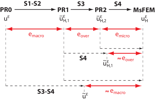
Refer to caption
Figure 6: Illustration of the strategy used to define indicators on each error source.

5.3 Adaptive algorithm

From the error estimate ηQsuperscript𝜂𝑄\eta^{Q} defined by (27) and the error indicators (ηmacroQsubscriptsuperscript𝜂𝑄𝑚𝑎𝑐𝑟𝑜\eta^{Q}_{macro}, ηoverQsubscriptsuperscript𝜂𝑄𝑜𝑣𝑒𝑟\eta^{Q}_{over}, ηmicroQsubscriptsuperscript𝜂𝑄𝑚𝑖𝑐𝑟𝑜\eta^{Q}_{micro}) defined in Section 5.2, we design a goal-oriented greedy adaptive algorithm that yields an adaptive MsFEM approach. The overall algorithm is presented in Fig. 7 and is similar to the algorithm designed in [19, Section 5.3] for the control of the MsFEM error measured in the energy norm.

The algorithm is based on a splitting (32) of the goal-oriented error estimator ηQsuperscript𝜂𝑄\eta^{Q} into local contributions {ηmacro,KQ,ηover,KQ,ηmicro,KQ}subscriptsuperscript𝜂𝑄𝑚𝑎𝑐𝑟𝑜𝐾subscriptsuperscript𝜂𝑄𝑜𝑣𝑒𝑟𝐾subscriptsuperscript𝜂𝑄𝑚𝑖𝑐𝑟𝑜𝐾\{\eta^{Q}_{macro,K},\eta^{Q}_{over,K},\eta^{Q}_{micro,K}\} in each element K𝐾K of the mesh 𝒯Hsubscript𝒯𝐻\mathcal{T}_{H}. These are used to mark coarse elements of the mesh 𝒯Hsubscript𝒯𝐻\mathcal{T}_{H} for further enrichment, and thus to drive the adaptive process by selecting optimal MsFEM parameters (HK,dK,hK)subscript𝐻𝐾subscript𝑑𝐾subscript𝐾(H_{K},d_{K},h_{K}) in each coarse region K𝐾K to compute both primal and adjoint approximate solutions.

Each iteration in the algorithm is made of three groups of computations: (i) microscale (possibly costly) computations that can be performed in the offline phase of the iteration; (ii) macroscale computations that can be performed in this offline phase; (iii) macroscale computations that need to be performed in the online phase of the iteration, but which are inexpensive.

1. Initialization 1.1 Set the tolerance error ηtolQsubscriptsuperscript𝜂𝑄𝑡𝑜𝑙\eta^{Q}_{tol} and the refinement parameter γrsubscript𝛾𝑟\gamma_{r} 1.2 Define a regular mesh 𝒯H(0)subscriptsuperscript𝒯0𝐻\mathcal{T}^{(0)}_{H} with uniform mesh size HK=Hsubscript𝐻𝐾𝐻H_{K}=H 1.3 Set loc(0)=glob(0)={all elements K of𝒯H(0)}subscriptsuperscript0𝑙𝑜𝑐subscriptsuperscript0𝑔𝑙𝑜𝑏all elements K ofsubscriptsuperscript𝒯0𝐻\mathcal{R}^{(0)}_{loc}=\mathcal{R}^{(0)}_{glob}=\{\text{all elements $K$ of}\;\mathcal{T}^{(0)}_{H}\} 1.4 Set SK=Ksubscript𝑆𝐾𝐾S_{K}=K and hK=HKsubscript𝐾subscript𝐻𝐾h_{K}=H_{K} for all elements K𝐾K of 𝒯H(0)subscriptsuperscript𝒯0𝐻\mathcal{T}^{(0)}_{H} 1.5 Set k=0𝑘0k=0 2. Increment kk+1𝑘𝑘1k\rightarrow k+1 3. MICROSCALE OFFLINE COMPUTATIONS 3.1 For all Kloc(k1)𝐾subscriptsuperscript𝑘1𝑙𝑜𝑐K\in\mathcal{R}^{(k-1)}_{loc}, solve the local problems (8) over SKsubscript𝑆𝐾S_{K} using a P1 discretization with mesh size hKsubscript𝐾h_{K}, in order to get the harmonic coordinates 𝒘ε,K(k)superscript𝒘𝜀𝐾𝑘\boldsymbol{w}^{\varepsilon,K(k)} (see Section 2.2.4) 3.2 Store the associated local stiffness matrices 4. MACROSCALE OFFLINE COMPUTATIONS 4.1 Define the new mesh 𝒯H(k)superscriptsubscript𝒯𝐻𝑘\mathcal{T}_{H}^{(k)} by refining each element Kglob(k1)𝐾subscriptsuperscript𝑘1𝑔𝑙𝑜𝑏K\in\mathcal{R}^{(k-1)}_{glob} using the local mesh size HKsubscript𝐻𝐾H_{K} 4.2 For all Kglob(k1)𝐾subscriptsuperscript𝑘1𝑔𝑙𝑜𝑏K\in\mathcal{R}^{(k-1)}_{glob}, define the new MsFEM basis functions ϕiε(k)superscriptsubscriptitalic-ϕ𝑖𝜀𝑘\phi_{i}^{\varepsilon(k)} from 𝒘ε,K(k)superscript𝒘𝜀𝐾𝑘\boldsymbol{w}^{\varepsilon,K(k)} 4.3 Solve the local problems associated to the computation of equilibrated flux fields (see Section 3.2) 4.4 Solve the local problems associated to the computation of error indicators (see Section 5.2) 5. MACROSCALE ONLINE COMPUTATIONS 5.1 Solve the global MsFEM problems to get (uHε(k),u~res,Hε(k))subscriptsuperscript𝑢𝜀𝑘𝐻subscriptsuperscript~𝑢𝜀𝑘𝑟𝑒𝑠𝐻(u^{\varepsilon(k)}_{H},\widetilde{u}^{\varepsilon(k)}_{res,H}), and deduce (u^Hε(k),u~^res,Hε(k))subscriptsuperscript^𝑢𝜀𝑘𝐻subscriptsuperscript^~𝑢𝜀𝑘𝑟𝑒𝑠𝐻\left(\widehat{u}^{\varepsilon(k)}_{H},\widehat{\widetilde{u}}^{\varepsilon(k)}_{res,H}\right) 5.2 Recover the equilibrated tractions and the admissible flux fields (𝒒^Hε(k),𝒒~^res,Hε(k))subscriptsuperscript^𝒒𝜀𝑘𝐻subscriptsuperscript^~𝒒𝜀𝑘𝑟𝑒𝑠𝐻\left(\widehat{\boldsymbol{q}}^{\varepsilon(k)}_{H},\widehat{\widetilde{\boldsymbol{q}}}^{\varepsilon(k)}_{res,H}\right) 5.3 Compute the global error estimate ηQ(k)superscript𝜂𝑄𝑘\eta^{Q(k)}. If ηQ(k)ηtolQsuperscript𝜂𝑄𝑘subscriptsuperscript𝜂𝑄𝑡𝑜𝑙\eta^{Q(k)}\leq\eta^{Q}_{tol}, then STOP; otherwise go to Step 5.4 5.4 Compute the indicators ηmacroQ(k)subscriptsuperscript𝜂𝑄𝑘𝑚𝑎𝑐𝑟𝑜\eta^{Q(k)}_{macro}, ηoverQ(k)subscriptsuperscript𝜂𝑄𝑘𝑜𝑣𝑒𝑟\eta^{Q(k)}_{over}, ηmicroQ(k)subscriptsuperscript𝜂𝑄𝑘𝑚𝑖𝑐𝑟𝑜\eta^{Q(k)}_{micro} and M=max(ηmacroQ(k),ηoverQ(k),ηmicroQ(k))𝑀subscriptsuperscript𝜂𝑄𝑘𝑚𝑎𝑐𝑟𝑜subscriptsuperscript𝜂𝑄𝑘𝑜𝑣𝑒𝑟subscriptsuperscript𝜂𝑄𝑘𝑚𝑖𝑐𝑟𝑜M=\max\left(\eta^{Q(k)}_{macro},\eta^{Q(k)}_{over},\eta^{Q(k)}_{micro}\right) 5.5 If M=ηmicroQ(k)𝑀subscriptsuperscript𝜂𝑄𝑘𝑚𝑖𝑐𝑟𝑜M=\eta^{Q(k)}_{micro}, set loc(k)=glob(k)={K𝒯H(k),ηmicro,KQ(k)|K|γrmaxK¯ηmicro,K¯Q(k)|K¯|}subscriptsuperscript𝑘𝑙𝑜𝑐subscriptsuperscript𝑘𝑔𝑙𝑜𝑏formulae-sequence𝐾superscriptsubscript𝒯𝐻𝑘subscriptsuperscript𝜂𝑄𝑘𝑚𝑖𝑐𝑟𝑜𝐾𝐾subscript𝛾𝑟¯𝐾subscriptsuperscript𝜂𝑄𝑘𝑚𝑖𝑐𝑟𝑜¯𝐾¯𝐾\mathcal{R}^{(k)}_{loc}=\mathcal{R}^{(k)}_{glob}=\left\{K\in\mathcal{T}_{H}^{(k)},\ \frac{\eta^{Q(k)}_{micro,K}}{|K|}\geq\gamma_{r}\,\underset{\overline{K}}{\max}\,\frac{\eta^{Q(k)}_{micro,\overline{K}}}{|\overline{K}|}\right\}, modify hKsubscript𝐾h_{K} for all Kloc(k)𝐾subscriptsuperscript𝑘𝑙𝑜𝑐K\in\mathcal{R}^{(k)}_{loc} and go to Step 2 5.6 If M=ηoverQ(k)𝑀subscriptsuperscript𝜂𝑄𝑘𝑜𝑣𝑒𝑟M=\eta^{Q(k)}_{over}, set loc(k)=glob(k)={K𝒯H(k),ηover,KQ(k)|K|γrmaxK¯ηover,K¯Q(k)|K¯|}subscriptsuperscript𝑘𝑙𝑜𝑐subscriptsuperscript𝑘𝑔𝑙𝑜𝑏formulae-sequence𝐾superscriptsubscript𝒯𝐻𝑘subscriptsuperscript𝜂𝑄𝑘𝑜𝑣𝑒𝑟𝐾𝐾subscript𝛾𝑟¯𝐾subscriptsuperscript𝜂𝑄𝑘𝑜𝑣𝑒𝑟¯𝐾¯𝐾\mathcal{R}^{(k)}_{loc}=\mathcal{R}^{(k)}_{glob}=\left\{K\in\mathcal{T}_{H}^{(k)},\ \frac{\eta^{Q(k)}_{over,K}}{|K|}\geq\gamma_{r}\,\underset{\overline{K}}{\max}\,\frac{\eta^{Q(k)}_{over,\overline{K}}}{|\overline{K}|}\right\}, modify dKsubscript𝑑𝐾d_{K} for all Kloc(k)𝐾subscriptsuperscript𝑘𝑙𝑜𝑐K\in\mathcal{R}^{(k)}_{loc} and go to Step 2 5.7 If M=ηmacroQ(k)𝑀subscriptsuperscript𝜂𝑄𝑘𝑚𝑎𝑐𝑟𝑜M=\eta^{Q(k)}_{macro}, set loc(k)=subscriptsuperscript𝑘𝑙𝑜𝑐\mathcal{R}^{(k)}_{loc}=\emptyset and glob(k)={K𝒯H(k),ηmacro,KQ(k)|K|γrmaxK¯ηmacro,K¯Q(k)|K¯|}subscriptsuperscript𝑘𝑔𝑙𝑜𝑏formulae-sequence𝐾superscriptsubscript𝒯𝐻𝑘subscriptsuperscript𝜂𝑄𝑘𝑚𝑎𝑐𝑟𝑜𝐾𝐾subscript𝛾𝑟¯𝐾subscriptsuperscript𝜂𝑄𝑘𝑚𝑎𝑐𝑟𝑜¯𝐾¯𝐾\mathcal{R}^{(k)}_{glob}=\left\{K\in\mathcal{T}_{H}^{(k)},\ \frac{\eta^{Q(k)}_{macro,K}}{|K|}\geq\gamma_{r}\,\underset{\overline{K}}{\max}\,\frac{\eta^{Q(k)}_{macro,\overline{K}}}{|\overline{K}|}\right\}, modify HKsubscript𝐻𝐾H_{K} for all Kglob(k)𝐾subscriptsuperscript𝑘𝑔𝑙𝑜𝑏K\in\mathcal{R}^{(k)}_{glob} and go to Step 2

Figure 7: Goal-oriented adaptive algorithm to drive the MsFEM computations.

The adaptive procedure is associated with the following considerations:

  • \bullet

    the algorithm is initialized with the coarsest MsFEM configuration that can be employed (regular coarse mesh, no oversampling, fine-scale problems solved with a single macro element). In this configuration, the diffusion tensor that locally appears to compute the MsFEM shape functions is the average of 𝔸εsuperscript𝔸𝜀\mathbb{A}^{\varepsilon} on K𝐾K, as discussed in [19, Remark 20];

  • \bullet

    when modifying the parameters hKsubscript𝐾h_{K} from their initial value hK=HKsubscript𝐾subscript𝐻𝐾h_{K}=H_{K} (in Step 5.5), two values are considered in the adaptive process: hK=ε/5subscript𝐾𝜀5h_{K}=\varepsilon/5 or hK=ε/20subscript𝐾𝜀20h_{K}=\varepsilon/20 (finest mesh size at the microscale);

  • \bullet

    when modifying the parameters dKsubscript𝑑𝐾d_{K} from their initial value dK=HKsubscript𝑑𝐾subscript𝐻𝐾d_{K}=H_{K} i.e. SK=Ksubscript𝑆𝐾𝐾S_{K}=K (in Step 5.6), the oversampling size is determined by adding layers of progressive thickness ε𝜀\varepsilon, 2ε2𝜀2\varepsilon, 3ε3𝜀3\varepsilon, …, around the element K𝐾K. Such an adaptation is not performed when hK=HKsubscript𝐾subscript𝐻𝐾h_{K}=H_{K};

  • \bullet

    refining the mesh 𝒯Hsubscript𝒯𝐻\mathcal{T}_{H}, i.e. modifying the parameters HKsubscript𝐻𝐾H_{K} (in Step 5.7), is performed using a quadtree (or octree in 3D) method with nested elements. This requires to handle hanging nodes;

  • \bullet

    the adapted parameters hKsubscript𝐾h_{K}, dKsubscript𝑑𝐾d_{K} and HKsubscript𝐻𝐾H_{K} are defined from classical adaptive strategies (see [42]), based on the convergence rates given by the a priori estimates (6) or (7), and with an error target ηmacro/over/microQ=ηtolQ/3subscriptsuperscript𝜂𝑄𝑚𝑎𝑐𝑟𝑜𝑜𝑣𝑒𝑟𝑚𝑖𝑐𝑟𝑜subscriptsuperscript𝜂𝑄𝑡𝑜𝑙3\eta^{Q}_{macro/over/micro}=\eta^{Q}_{tol}/3;

  • \bullet

    the technique proposed in [5] and based on composition rules (see Section 2.2.4) is beneficially used throughout the adaptive process. It enables independent computations without coming back to the fine scale offline computations (no additional costly computations). The technique is used in its p𝑝p-refinement version in Steps 4.3 and 4.4, while it is used in its H𝐻H-refinement version in Step 4.2 (when the macro mesh has to be refined). In short, this technique allows us to refine the coarse mesh without the need to solve new fine-scale problems of the type (8).

The adaptive algorithm allows us to adjust automatically (and hopefully optimally) the calculation parameters during the simulation. We expect that it provides MsFEM parameters which ensure a correct balance between computational cost and accuracy on the output of interest. In particular, it should lead to fine-scale solutions only in the parts of ΩΩ\Omega which have an impact on the value of the quantity of interest. As will be shown below, and as expected, it also leads (for the same tolerance on the error) to less expensive computations than the adaptive algorithm introduced in [19] to drive the MsFEM computations according to the error measured in the energy norm.

6 Numerical results

We consider two test-cases. The first one corresponds to a structure with a local defect, for which we consider two possible loadings (see Section 6.1). The second one is a flow problem in fractured porous media (see Section 6.2), which has already been considered in [20]. For all these test-cases, the conclusions of our numerical investigations are the same:

  • 1.

    It is worth working with a goal-oriented adaptive strategy rather than an adaptive strategy based on the global error: for the same error tolerance, the computational cost is much lower, in the sense that the obtained mesh (satisfying the prescribed error tolerance) is much coarser.

  • 2.

    As the mesh is iteratively adapted, the error on the quantity of interest monotically decreases until reaching the prescribed tolerance.

  • 3.

    The error estimate ηQsuperscript𝜂𝑄\eta^{Q} is always an upper bound on the exact error, in view of (27). We see below that it only slightly overestimates the error (roughly by 10% on the considered numerical examples), showing thus its accuracy.

6.1 Structure with a local defect

To start with, we consider a highly oscillatory problem with defects, as introduced and analyzed in details in [10, 11, 12] (see also the recent works [13, 14]). We assume that the oscillating coefficient is a local perturbation (which models the defect) of a function with simple geometric properties, for instance a periodic function. We thus consider problem (1) with a (scalar, to simplify) coefficient Aε(𝒙)=a(𝒙/ε)superscript𝐴𝜀𝒙𝑎𝒙𝜀A^{\varepsilon}(\boldsymbol{x})=a(\boldsymbol{x}/\varepsilon) with a=aper+b𝑎subscript𝑎𝑝𝑒𝑟𝑏a=a_{per}+b where bLr(d)𝑏superscript𝐿𝑟superscript𝑑b\in L^{r}(\mathbb{R}^{d}) is the local perturbation. The homogenization of such a problem is addressed in [10] for the Hilbertian case r=2𝑟2r=2 and in [11, 12] for the cases 1<r<+1𝑟1<r<+\infty (see also [13, 14]). In general, the defect does not modify the macroscopic behavior (i.e. the homogenized solution) but it affects the solution locally, and at the small scale.

Inspired by these works, we consider here the following example. We set Ω=(1,1)2Ωsuperscript1.12\Omega=(-1,1)^{2}, choose ε=1/N𝜀1𝑁\varepsilon=1/N for some integer N𝑁N, and consider problem (1) with 𝔸ε(𝒙)=Aε(𝒙)𝕀superscript𝔸𝜀𝒙superscript𝐴𝜀𝒙𝕀\mathbb{A}^{\varepsilon}(\boldsymbol{x})=A^{\varepsilon}(\boldsymbol{x})\mathbb{I}, where Aε(𝒙)=aper(𝒙/ε)+b(𝒙/ε)superscript𝐴𝜀𝒙subscript𝑎𝑝𝑒𝑟𝒙𝜀𝑏𝒙𝜀A^{\varepsilon}(\boldsymbol{x})=a_{per}(\boldsymbol{x}/\varepsilon)+b(\boldsymbol{x}/\varepsilon) with

aper(x1,x2)=3+cos(2πx1)+cos(2πx2),b(x1,x2)=5exp((x12+x22)).formulae-sequencesubscript𝑎𝑝𝑒𝑟subscript𝑥1subscript𝑥232𝜋subscript𝑥12𝜋subscript𝑥2𝑏subscript𝑥1subscript𝑥25superscriptsubscript𝑥12superscriptsubscript𝑥22a_{per}(x_{1},x_{2})=3+\cos(2\pi x_{1})+\cos(2\pi x_{2}),\qquad b(x_{1},x_{2})=5\exp(-(x_{1}^{2}+x_{2}^{2})).

In the following, we choose ε=1/20𝜀120\varepsilon=1/20. The evolution of Aεsuperscript𝐴𝜀A^{\varepsilon} is shown on Fig. 8.

Refer to caption
Refer to caption
Figure 8: Defect problem: evolution of Aεsuperscript𝐴𝜀A^{\varepsilon}, modeling a defect, in the domain ΩΩ\Omega (we set ε=1/20𝜀120\varepsilon=1/20).

6.1.1 Sinusoidal loading

We first consider the loading f(x1,x2)=sin(πx1)cos(πx2)𝑓subscript𝑥1subscript𝑥2𝜋subscript𝑥1𝜋subscript𝑥2f(x_{1},x_{2})=\sin(\pi x_{1})\cos(\pi x_{2}). We take an initial mesh 𝒯Hsubscript𝒯𝐻\mathcal{T}_{H} made of 9×9999\times 9 macro elements, with hK=ε/3subscript𝐾𝜀3h_{K}=\varepsilon/3 for any K𝐾K and no oversampling. The approximate MsFEM solution uHεsubscriptsuperscript𝑢𝜀𝐻u^{\varepsilon}_{H} is represented below and compared to the exact solution uεsuperscript𝑢𝜀u^{\varepsilon}, which is obtained in practice through an expensive computation over a 500×500500500500\times 500 fine mesh. The solutions uεsuperscript𝑢𝜀u^{\varepsilon} and uHεsubscriptsuperscript𝑢𝜀𝐻u^{\varepsilon}_{H} are shown on Fig. 9, the gradients uεbold-∇superscript𝑢𝜀\boldsymbol{\nabla}u^{\varepsilon} and uHεbold-∇subscriptsuperscript𝑢𝜀𝐻\boldsymbol{\nabla}u^{\varepsilon}_{H} are shown on Fig. 10, and the fluxes 𝒒εsuperscript𝒒𝜀\boldsymbol{q}^{\varepsilon} and 𝒒Hεsubscriptsuperscript𝒒𝜀𝐻\boldsymbol{q}^{\varepsilon}_{H} are shown on Fig. 11. We also show the distribution of the energy of the exact solution and of the global error on Fig. 12.
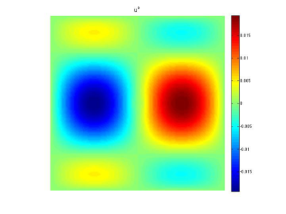
Refer to caption
Refer to caption
Figure 9: Defect problem, sinusoidal loading: exact solution uεsuperscript𝑢𝜀u^{\varepsilon} (left) and MsFEM solution uHεsubscriptsuperscript𝑢𝜀𝐻u^{\varepsilon}_{H} (right).
Refer to caption
Refer to caption
Refer to caption
Refer to caption
Figure 10: Defect problem, sinusoidal loading: exact gradient uεbold-∇superscript𝑢𝜀\boldsymbol{\nabla}u^{\varepsilon} (left) and MsFEM gradient uHεbold-∇subscriptsuperscript𝑢𝜀𝐻\boldsymbol{\nabla}u^{\varepsilon}_{H} (right) (top row: components uε𝒆1bold-∇superscript𝑢𝜀subscript𝒆1\boldsymbol{\nabla}u^{\varepsilon}\cdot\boldsymbol{e}_{1} and uHε𝒆1bold-∇superscriptsubscript𝑢𝐻𝜀subscript𝒆1\boldsymbol{\nabla}u_{H}^{\varepsilon}\cdot\boldsymbol{e}_{1}; bottom row: components uε𝒆2bold-∇superscript𝑢𝜀subscript𝒆2\boldsymbol{\nabla}u^{\varepsilon}\cdot\boldsymbol{e}_{2} and uHε𝒆2bold-∇superscriptsubscript𝑢𝐻𝜀subscript𝒆2\boldsymbol{\nabla}u_{H}^{\varepsilon}\cdot\boldsymbol{e}_{2}).
Refer to caption
Refer to caption
Refer to caption
Refer to caption
Figure 11: Defect problem, sinusoidal loading: exact flux 𝒒εsuperscript𝒒𝜀\boldsymbol{q}^{\varepsilon} (left) and MsFEM flux 𝒒Hεsubscriptsuperscript𝒒𝜀𝐻\boldsymbol{q}^{\varepsilon}_{H} (right) (top row: components 𝒒ε𝒆1superscript𝒒𝜀subscript𝒆1\boldsymbol{q}^{\varepsilon}\cdot\boldsymbol{e}_{1} and 𝒒Hε𝒆1superscriptsubscript𝒒𝐻𝜀subscript𝒆1\boldsymbol{q}_{H}^{\varepsilon}\cdot\boldsymbol{e}_{1}; bottom row: components 𝒒ε𝒆2superscript𝒒𝜀subscript𝒆2\boldsymbol{q}^{\varepsilon}\cdot\boldsymbol{e}_{2} and 𝒒Hε𝒆2superscriptsubscript𝒒𝐻𝜀subscript𝒆2\boldsymbol{q}_{H}^{\varepsilon}\cdot\boldsymbol{e}_{2}).
Refer to caption
Refer to caption
Figure 12: Defect problem, sinusoidal loading: distribution of the energy of the exact solution (left) and of the global error (right).

We also show on Fig. 13 the distribution of the error on uεsuperscript𝑢𝜀u^{\varepsilon}, uε𝒆1bold-∇superscript𝑢𝜀subscript𝒆1\boldsymbol{\nabla}u^{\varepsilon}\cdot\boldsymbol{e}_{1} and 𝒒ε𝒆1superscript𝒒𝜀subscript𝒆1\boldsymbol{q}^{\varepsilon}\cdot\boldsymbol{e}_{1}.

Refer to caption
Refer to caption
Refer to caption
Figure 13: Defect problem, sinusoidal loading: error between exact and MsFEM fields for uεsuperscript𝑢𝜀u^{\varepsilon} (left), uε𝒆1bold-∇superscript𝑢𝜀subscript𝒆1\boldsymbol{\nabla}u^{\varepsilon}\cdot\boldsymbol{e}_{1} (center) and 𝒒ε𝒆1superscript𝒒𝜀subscript𝒆1\boldsymbol{q}^{\varepsilon}\cdot\boldsymbol{e}_{1} (right).

We choose the quantity of interest Q(uε)=1|ω|ω𝒒ε𝒆1=1|ω|ω𝒆1𝔸εuε𝑄superscript𝑢𝜀1𝜔subscript𝜔superscript𝒒𝜀subscript𝒆11𝜔subscript𝜔subscript𝒆1superscript𝔸𝜀bold-∇superscript𝑢𝜀\displaystyle Q(u^{\varepsilon})=\frac{1}{|\omega|}\int_{\omega}\boldsymbol{q}^{\varepsilon}\cdot\boldsymbol{e}_{1}=\frac{1}{|\omega|}\int_{\omega}\boldsymbol{e}_{1}\cdot\mathbb{A}^{\varepsilon}\boldsymbol{\nabla}u^{\varepsilon} with |ω|=4ε×4ε𝜔4𝜀4𝜀|\omega|=4\varepsilon\times 4\varepsilon. We consider two cases:

  • 1.

    Case 1: the subregion ω𝜔\omega is centered on the defect (Q=Q1𝑄subscript𝑄1Q=Q_{1});

  • 2.

    Case 2: the subregion ω𝜔\omega is far from the defect (Q=Q2𝑄subscript𝑄2Q=Q_{2}).

Note that uεsuperscript𝑢𝜀u^{\varepsilon} is close to zero in the region around the defect (see Fig. 9), so considering as quantity of interest the average of uεsuperscript𝑢𝜀u^{\varepsilon} would not be interesting. In contrast, 𝒒ε𝒆1superscript𝒒𝜀subscript𝒆1\boldsymbol{q}^{\varepsilon}\cdot\boldsymbol{e}_{1} is not close to zero in that region (see Fig. 11). The adjoint solutions u~εsuperscript~𝑢𝜀\widetilde{u}^{\varepsilon} and fluxes 𝒒~εsuperscript~𝒒𝜀\widetilde{\boldsymbol{q}}^{\varepsilon} corresponding to the quantities of interest Q1subscript𝑄1Q_{1} and Q2subscript𝑄2Q_{2} are shown on Figs. 14 and 15. We observe, as expected, that the adjoint solutions are essentially supported in the domain of interest ω𝜔\omega.

Refer to caption
Refer to caption
Figure 14: Defect problem, sinusoidal loading: exact adjoint solution u~εsuperscript~𝑢𝜀\widetilde{u}^{\varepsilon} for Q1subscript𝑄1Q_{1} (left) and Q2subscript𝑄2Q_{2} (right).
Refer to caption
Refer to caption
Refer to caption
Refer to caption
Figure 15: Defect problem, sinusoidal loading: exact adjoint flux 𝒒~εsuperscript~𝒒𝜀\widetilde{\boldsymbol{q}}^{\varepsilon} for Q1subscript𝑄1Q_{1} (left) and Q2subscript𝑄2Q_{2} (right) (top row: component along 𝒆1subscript𝒆1\boldsymbol{e}_{1}; bottom row: component along 𝒆2subscript𝒆2\boldsymbol{e}_{2}).

The error threshold is fixed to 1%percent11\%. We show on Fig. 16 (resp. Fig. 17) the final MsFEM discretization obtained after using the adaptive algorithm presented in Section 5.3, in order to respect the error threshold for the quantity of interest Q1subscript𝑄1Q_{1} (resp. Q2subscript𝑄2Q_{2}). This discretization is to be compared with that obtained when controlling the global error (in energy norm) using the tools presented in [19], which is shown on Fig. 18. Obviously, the mesh on Figs. 16 and 17 is much coarser than the mesh on Fig. 18. This shows, as expected, that it is worth working with a goal-oriented adaptive strategy, rather than an adaptive strategy based on the global error: for the same error, the computational cost is much lower. Comparing Figs. 16 and 17, we also observe that the mesh is only refined close to the region of interest ω𝜔\omega. In the second example, when this region is far from the defect, it is not needed to adapt the mesh close to the defect.

As regards the accuracy of the error estimate (with respect to the actual error), we observe that ηQ/|Q(uε)Q(uHε)|=1.11superscript𝜂𝑄𝑄superscript𝑢𝜀𝑄subscriptsuperscript𝑢𝜀𝐻111\eta^{Q}/|Q(u^{\varepsilon})-Q(u^{\varepsilon}_{H})|=1.11 (resp. 1.13) at the first iteration of the adaptive algorithm, and ηQ/|Q(uε)Q(uHε)|=1.07superscript𝜂𝑄𝑄superscript𝑢𝜀𝑄subscriptsuperscript𝑢𝜀𝐻107\eta^{Q}/|Q(u^{\varepsilon})-Q(u^{\varepsilon}_{H})|=1.07 (resp. 1.06) at the final iteration of the adaptive algorithm, for the quantities of interest Q1subscript𝑄1Q_{1} and Q2subscript𝑄2Q_{2}, respectively. As pointed out above, the error estimate thus only very slightly overestimates the actual error.

Refer to caption
Figure 16: Defect problem, sinusoidal loading: final MsFEM discretization for Q1subscript𝑄1Q_{1} (left: coarse mesh; center: oversampling size; right: fine mesh size hKsubscript𝐾h_{K}).
Refer to caption
Figure 17: Defect problem, sinusoidal loading: final MsFEM discretization for Q2subscript𝑄2Q_{2}.
Refer to caption
Figure 18: Defect problem, sinusoidal loading: Final MsFEM discretization when controlling the global error.

We eventually show on Fig. 19 the convergence of the error estimate on Q𝑄Q with respect to the iterations of the adaptive process. As the iterations proceed, the error (which is initially close to 25%, due purposely to the coarse mesh that is used) monotically decreases until reaching the prescribed tolerance of 1% in about 10 iterations. We also show on Fig. 20 the evolution of the error indicators along the adaptive process. We observe that, for this case, the fine mesh is first refined before adapting the coarse mesh and finally extending the oversampling zone.
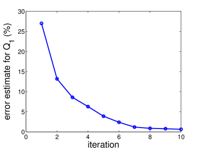
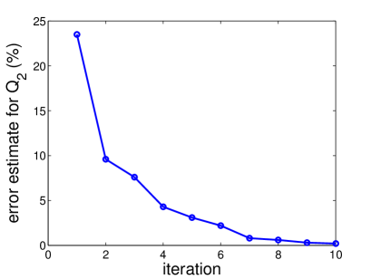
Refer to caption
Refer to caption
Figure 19: Defect problem, sinusoidal loading: convergence of the error estimate for Q1subscript𝑄1Q_{1} (left) and Q2subscript𝑄2Q_{2} (right).
Refer to caption
Refer to caption
Figure 20: Defect problem, sinusoidal loading: convergence of the error indicators for Q1subscript𝑄1Q_{1} (left) and Q2subscript𝑄2Q_{2} (right).

6.1.2 Exponential loading

With the aim to consider a quantity of interest that depends on uεsuperscript𝑢𝜀u^{\varepsilon} (and not on the flux 𝒒εsuperscript𝒒𝜀\boldsymbol{q}^{\varepsilon} as in the previous example), we consider here a different loading: f(x1,x2)=exp((x12+x22))𝑓subscript𝑥1subscript𝑥2superscriptsubscript𝑥12superscriptsubscript𝑥22f(x_{1},x_{2})=\exp(-(x_{1}^{2}+x_{2}^{2})). We again take an initial mesh 𝒯Hsubscript𝒯𝐻\mathcal{T}_{H} made of 9×9999\times 9 macro elements, with hK=ε/3subscript𝐾𝜀3h_{K}=\varepsilon/3 for any K𝐾K and without any oversampling. The reference solution is computed on a 500×500500500500\times 500 fine mesh. The MsFEM solution uHεsubscriptsuperscript𝑢𝜀𝐻u^{\varepsilon}_{H} is compared to the reference solution uεsuperscript𝑢𝜀u^{\varepsilon} on Fig. 21, their gradients uHεbold-∇subscriptsuperscript𝑢𝜀𝐻\boldsymbol{\nabla}u^{\varepsilon}_{H} and uεbold-∇superscript𝑢𝜀\boldsymbol{\nabla}u^{\varepsilon} on Fig. 22, and fluxes 𝒒Hεsubscriptsuperscript𝒒𝜀𝐻\boldsymbol{q}^{\varepsilon}_{H} and 𝒒εsuperscript𝒒𝜀\boldsymbol{q}^{\varepsilon} on Fig. 23. We also represent the distribution of the energy of the exact solution and of the global error on Fig. 24. In contrast to the previous test-case, uεsuperscript𝑢𝜀u^{\varepsilon} is not close to 0 in the zone where the defect is located (see Fig. 21). This is thus a relevant test-case for considering as quantity of interest the average of uεsuperscript𝑢𝜀u^{\varepsilon} in that zone.

Refer to caption
Refer to caption
Figure 21: Defect problem, exponential loading: exact solution uεsuperscript𝑢𝜀u^{\varepsilon} (left) and MsFEM solution uHεsubscriptsuperscript𝑢𝜀𝐻u^{\varepsilon}_{H} (right).
Refer to caption
Refer to caption
Refer to caption
Refer to caption
Figure 22: Defect problem, exponential loading: exact gradient uεbold-∇superscript𝑢𝜀\boldsymbol{\nabla}u^{\varepsilon} (left) and MsFEM gradient uHεbold-∇subscriptsuperscript𝑢𝜀𝐻\boldsymbol{\nabla}u^{\varepsilon}_{H} (right) (top row: components uε𝒆1bold-∇superscript𝑢𝜀subscript𝒆1\boldsymbol{\nabla}u^{\varepsilon}\cdot\boldsymbol{e}_{1} and uHε𝒆1bold-∇superscriptsubscript𝑢𝐻𝜀subscript𝒆1\boldsymbol{\nabla}u_{H}^{\varepsilon}\cdot\boldsymbol{e}_{1}; bottom row: components uε𝒆2bold-∇superscript𝑢𝜀subscript𝒆2\boldsymbol{\nabla}u^{\varepsilon}\cdot\boldsymbol{e}_{2} and uHε𝒆2bold-∇superscriptsubscript𝑢𝐻𝜀subscript𝒆2\boldsymbol{\nabla}u_{H}^{\varepsilon}\cdot\boldsymbol{e}_{2}).
Refer to caption
Refer to caption
Refer to caption
Refer to caption
Figure 23: Defect problem, exponential loading: exact flux 𝒒εsuperscript𝒒𝜀\boldsymbol{q}^{\varepsilon} (left) and MsFEM flux 𝒒Hεsubscriptsuperscript𝒒𝜀𝐻\boldsymbol{q}^{\varepsilon}_{H} (right) (top row: components 𝒒ε𝒆1superscript𝒒𝜀subscript𝒆1\boldsymbol{q}^{\varepsilon}\cdot\boldsymbol{e}_{1} and 𝒒Hε𝒆1superscriptsubscript𝒒𝐻𝜀subscript𝒆1\boldsymbol{q}_{H}^{\varepsilon}\cdot\boldsymbol{e}_{1}; bottom row: components 𝒒ε𝒆2superscript𝒒𝜀subscript𝒆2\boldsymbol{q}^{\varepsilon}\cdot\boldsymbol{e}_{2} and 𝒒Hε𝒆2superscriptsubscript𝒒𝐻𝜀subscript𝒆2\boldsymbol{q}_{H}^{\varepsilon}\cdot\boldsymbol{e}_{2}).
Refer to caption
Refer to caption
Figure 24: Defect problem, exponential loading: distribution of the energy of the exact solution (left) and of the global error (right).

We also plot on Fig. 25 the distribution of the error on uεsuperscript𝑢𝜀u^{\varepsilon}, uε𝒆1bold-∇superscript𝑢𝜀subscript𝒆1\boldsymbol{\nabla}u^{\varepsilon}\cdot\boldsymbol{e}_{1} and 𝒒ε𝒆1superscript𝒒𝜀subscript𝒆1\boldsymbol{q}^{\varepsilon}\cdot\boldsymbol{e}_{1}.

Refer to caption
Refer to caption
Refer to caption
Figure 25: Defect problem, exponential loading: error between exact and MsFEM fields for uεsuperscript𝑢𝜀u^{\varepsilon} (left), uε𝒆1bold-∇superscript𝑢𝜀subscript𝒆1\boldsymbol{\nabla}u^{\varepsilon}\cdot\boldsymbol{e}_{1} (center) and 𝒒ε𝒆1superscript𝒒𝜀subscript𝒆1\boldsymbol{q}^{\varepsilon}\cdot\boldsymbol{e}_{1} (right).

As pointed out above, we choose the quantity of interest Q(uε)=1|ω|ωuε𝑄superscript𝑢𝜀1𝜔subscript𝜔superscript𝑢𝜀\displaystyle Q(u^{\varepsilon})=\frac{1}{|\omega|}\int_{\omega}u^{\varepsilon} with |ω|=4ε×4ε𝜔4𝜀4𝜀|\omega|=4\varepsilon\times 4\varepsilon. We consider two cases:

  • 1.

    Case 1: the subregion ω𝜔\omega is centered on the defect (Q=Q1𝑄subscript𝑄1Q=Q_{1});

  • 2.

    Case 2: the subregion ω𝜔\omega is far from the defect (Q=Q2𝑄subscript𝑄2Q=Q_{2}).

The corresponding adjoint solutions u~εsuperscript~𝑢𝜀\widetilde{u}^{\varepsilon} and fluxes 𝒒~εsuperscript~𝒒𝜀\widetilde{\boldsymbol{q}}^{\varepsilon} are shown on Figs. 26 and 27. Again, as expected, the adjoint solutions are essentially supported in the domain of interest ω𝜔\omega.

Refer to caption
Refer to caption
Figure 26: Defect problem, exponential loading: exact adjoint solution u~εsuperscript~𝑢𝜀\widetilde{u}^{\varepsilon} for Q1subscript𝑄1Q_{1} (left) and Q2subscript𝑄2Q_{2} (right).
Refer to caption
Refer to caption
Refer to caption
Refer to caption
Figure 27: Defect problem, exponential loading: exact adjoint flux 𝒒~εsuperscript~𝒒𝜀\widetilde{\boldsymbol{q}}^{\varepsilon} for Q1subscript𝑄1Q_{1} (left) and Q2subscript𝑄2Q_{2} (right) (top row: component along 𝒆1subscript𝒆1\boldsymbol{e}_{1}; bottom row: component along 𝒆2subscript𝒆2\boldsymbol{e}_{2}).

The error threshold is fixed to 1%percent11\%. We show on Fig. 28 (resp. Fig. 29) the final MsFEM discretization obtained after using the adaptive algorithm presented in Section 5.3, in order to respect the error threshold for the quantity of interest Q1subscript𝑄1Q_{1} (resp. Q2subscript𝑄2Q_{2}). This discretization can be compared with that obtained when controlling the global error (in energy norm) using the tools presented in [19], which is shown on Fig. 30. The conclusions are the same as in the case of sinusoidal loading (see Section 6.1.1): (i) it is worth working with a goal-oriented adaptive strategy rather than with an adaptive strategy based on the global error and (ii) the mesh needs to be refined only in the region close to the region of interest ω𝜔\omega.

As regards the accuracy of the error estimate, we again observe that it is very good with only a slight overestimation of the error. Computations yield ηQ/|Q(uε)Q(uHε)|=1.14superscript𝜂𝑄𝑄superscript𝑢𝜀𝑄subscriptsuperscript𝑢𝜀𝐻114\eta^{Q}/|Q(u^{\varepsilon})-Q(u^{\varepsilon}_{H})|=1.14 (resp. 1.15) at the first iteration of the adaptive algorithm, and ηQ/|Q(uε)Q(uHε)|=1.07superscript𝜂𝑄𝑄superscript𝑢𝜀𝑄subscriptsuperscript𝑢𝜀𝐻107\eta^{Q}/|Q(u^{\varepsilon})-Q(u^{\varepsilon}_{H})|=1.07 (resp. 1.04) at the final iteration of the adaptive algorithm, for the quantities of interest Q1subscript𝑄1Q_{1} and Q2subscript𝑄2Q_{2}, respectively.

Refer to caption
Figure 28: Defect problem, exponential loading: final MsFEM discretization for Q1subscript𝑄1Q_{1}.
Refer to caption
Figure 29: Defect problem, exponential loading: final MsFEM discretization for Q2subscript𝑄2Q_{2}.
Refer to caption
Figure 30: Defect problem, exponential loading: final MsFEM discretization when controlling the global error.

We show on Fig. 31 how the error estimate on Q𝑄Q decreases as the adaptive iterations of the mesh proceed. For instance, after the first adaptation, the error has been divided by a factor 2, going from 80% to 50% for Q1subscript𝑄1Q_{1} (resp. 40% to 20% for Q2subscript𝑄2Q_{2}).

Refer to caption
Refer to caption
Figure 31: Defect problem, exponential loading: convergence of the error estimate for Q1subscript𝑄1Q_{1} (left) and Q2subscript𝑄2Q_{2} (right).

6.2 Flow problem

We now consider a flow problem in a fractured porous medium, with a source and a sink. This problem has already been considered in [20], with different multiscale techniques. The conductivity within the fractures can be several orders of magnitude higher than the conductivity within the matrix. In flow applications, one needs to obtain a good approximation of the pressure in a neighborhood of the wells.

We consider the domain Ω=(0,1)2Ωsuperscript0.12\Omega=(0,1)^{2} and the inflow-outflow source term f=χK1χK2𝑓subscript𝜒subscript𝐾1subscript𝜒subscript𝐾2f=\chi_{K_{1}}-\chi_{K_{2}} , where K1=[0.1,0.2]×[0.8,0.9]subscript𝐾1delimited-[]01.02delimited-[]08.09K_{1}=[0.1,0.2]\times[0.8,0.9] and K2=[0.8,0.9]×[0.1,0.2]subscript𝐾2delimited-[]08.09delimited-[]01.02K_{2}=[0.8,0.9]\times[0.1,0.2]. The pressure uεsuperscript𝑢𝜀u^{\varepsilon} is solution to

(Aεuε)=fin Ω,uε=0on Ω,formulae-sequencebold-∇superscript𝐴𝜀bold-∇superscript𝑢𝜀𝑓in Ωsuperscript𝑢𝜀0on Ω-\boldsymbol{\nabla}\cdot(A^{\varepsilon}\boldsymbol{\nabla}u^{\varepsilon})=f\ \ \text{in $\Omega$},\qquad u^{\varepsilon}=0\ \ \text{on $\partial\Omega$},

and we consider the quantity of interest Q(uε)=1|K2|K2uε𝑄superscript𝑢𝜀1subscript𝐾2subscriptsubscript𝐾2superscript𝑢𝜀\displaystyle Q(u^{\varepsilon})=\frac{1}{|K_{2}|}\int_{K_{2}}u^{\varepsilon}, that is the average value of the solution (i.e. the pressure) on the outflow region K2subscript𝐾2K_{2} (where the well is located).

The scalar-valued high-contrast function Aε(𝒙)superscript𝐴𝜀𝒙A^{\varepsilon}(\boldsymbol{x}) is shown on Fig. 32. We observe a high-conductivity channel crossing the domain ΩΩ\Omega, and separating the inflow and outflow regions. In the blue region, we have Aε=1superscript𝐴𝜀1A^{\varepsilon}=1, and in the red region we set Aε=104superscript𝐴𝜀superscript104A^{\varepsilon}=10^{4}. The contrast between the conductivities in the blue and red regions is thus very large.
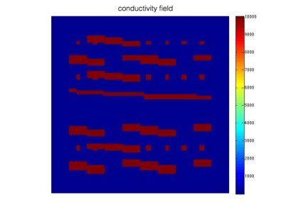
Refer to caption
Figure 32: Flow problem: evolution of Aεsuperscript𝐴𝜀A^{\varepsilon} in the domain ΩΩ\Omega.

We take an initial mesh 𝒯Hsubscript𝒯𝐻\mathcal{T}_{H} made of 10×10101010\times 10 macro elements, with hK=H/10subscript𝐾𝐻10h_{K}=H/10 for any K𝐾K and no oversampling. We show on Figs 33, 34 and 35 the exact solution uεsuperscript𝑢𝜀u^{\varepsilon} and its MsFEM approximation uHεsubscriptsuperscript𝑢𝜀𝐻u^{\varepsilon}_{H}, their gradients uεbold-∇superscript𝑢𝜀\boldsymbol{\nabla}u^{\varepsilon} and uHεbold-∇subscriptsuperscript𝑢𝜀𝐻\boldsymbol{\nabla}u^{\varepsilon}_{H}, and the fluxes 𝒒εsuperscript𝒒𝜀\boldsymbol{q}^{\varepsilon} and 𝒒Hεsubscriptsuperscript𝒒𝜀𝐻\boldsymbol{q}^{\varepsilon}_{H}. We can see that the solution uεsuperscript𝑢𝜀u^{\varepsilon} is essentially supported in the source region K1subscript𝐾1K_{1} and the sink region K2subscript𝐾2K_{2}. The initial approximation uHεsubscriptsuperscript𝑢𝜀𝐻u^{\varepsilon}_{H} is not very accurate, especially in the top half of ΩΩ\Omega. As can be seen on Fig. 40, the initial error on the quantity of interest is almost 60%. The discretization is purposely too coarse.
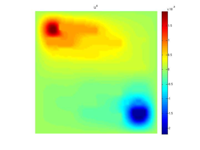
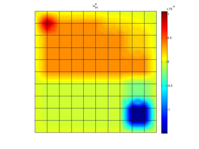
Refer to caption
Refer to caption
Figure 33: Flow problem: exact solution uεsuperscript𝑢𝜀u^{\varepsilon} (left) and MsFEM solution uHεsubscriptsuperscript𝑢𝜀𝐻u^{\varepsilon}_{H} (right).
Refer to caption
Refer to caption
Refer to caption
Refer to caption
Figure 34: Flow problem: exact gradient uεbold-∇superscript𝑢𝜀\boldsymbol{\nabla}u^{\varepsilon} (left) and MsFEM gradient uHεbold-∇subscriptsuperscript𝑢𝜀𝐻\boldsymbol{\nabla}u^{\varepsilon}_{H} (right) (top row: components uε𝒆1bold-∇superscript𝑢𝜀subscript𝒆1\boldsymbol{\nabla}u^{\varepsilon}\cdot\boldsymbol{e}_{1} and uHε𝒆1bold-∇superscriptsubscript𝑢𝐻𝜀subscript𝒆1\boldsymbol{\nabla}u_{H}^{\varepsilon}\cdot\boldsymbol{e}_{1}; bottom row: components uε𝒆2bold-∇superscript𝑢𝜀subscript𝒆2\boldsymbol{\nabla}u^{\varepsilon}\cdot\boldsymbol{e}_{2} and uHε𝒆2bold-∇superscriptsubscript𝑢𝐻𝜀subscript𝒆2\boldsymbol{\nabla}u_{H}^{\varepsilon}\cdot\boldsymbol{e}_{2}).
Refer to caption
Refer to caption
Refer to caption
Refer to caption
Figure 35: Flow problem: exact flux 𝒒εsuperscript𝒒𝜀\boldsymbol{q}^{\varepsilon} (left) and MsFEM flux 𝒒Hεsubscriptsuperscript𝒒𝜀𝐻\boldsymbol{q}^{\varepsilon}_{H} (right) (top row: components 𝒒ε𝒆1superscript𝒒𝜀subscript𝒆1\boldsymbol{q}^{\varepsilon}\cdot\boldsymbol{e}_{1} and 𝒒Hε𝒆1superscriptsubscript𝒒𝐻𝜀subscript𝒆1\boldsymbol{q}_{H}^{\varepsilon}\cdot\boldsymbol{e}_{1}; bottom row: components 𝒒ε𝒆2superscript𝒒𝜀subscript𝒆2\boldsymbol{q}^{\varepsilon}\cdot\boldsymbol{e}_{2} and 𝒒Hε𝒆2superscriptsubscript𝒒𝐻𝜀subscript𝒆2\boldsymbol{q}_{H}^{\varepsilon}\cdot\boldsymbol{e}_{2}).

The error between the exact solution and its MsFEM approximation is shown on Fig. 36.
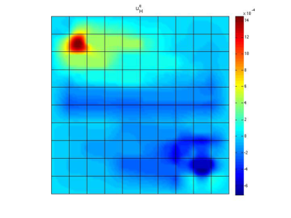
Refer to caption
Refer to caption
Figure 36: Flow problem: distribution of the error. Left: uεuHεsuperscript𝑢𝜀subscriptsuperscript𝑢𝜀𝐻u^{\varepsilon}-u^{\varepsilon}_{H}. Right: error in the energy norm.

The adjoint solution u~εsuperscript~𝑢𝜀\widetilde{u}^{\varepsilon} and flux 𝒒~εsuperscript~𝒒𝜀\widetilde{\boldsymbol{q}}^{\varepsilon} corresponding to the quantity of interest Q𝑄Q are shown on Fig. 37.

Refer to caption
Refer to caption
Refer to caption
Figure 37: Flow problem: exact adjoint solution u~εsuperscript~𝑢𝜀\widetilde{u}^{\varepsilon} (left), exact adjoint flux 𝒒~ε𝒆1superscript~𝒒𝜀subscript𝒆1\widetilde{\boldsymbol{q}}^{\varepsilon}\cdot\boldsymbol{e}_{1} (center) and 𝒒~ε𝒆2superscript~𝒒𝜀subscript𝒆2\widetilde{\boldsymbol{q}}^{\varepsilon}\cdot\boldsymbol{e}_{2} (right).

The error threshold is fixed to 1%percent11\%. We show on Fig. 38 the final MsFEM discretization that we obtain in order to respect the error threshold for the quantity of interest. As in the previous test cases, this discretization is much coarser than the discretization (shown on Fig. 39) that is obtained when controlling the global error (in energy norm) using tools presented in [19].

The accuracy of the error estimate is again very good in this example. We get ηQ/|Q(uε)Q(uHε)|=1.14superscript𝜂𝑄𝑄superscript𝑢𝜀𝑄subscriptsuperscript𝑢𝜀𝐻114\eta^{Q}/|Q(u^{\varepsilon})-Q(u^{\varepsilon}_{H})|=1.14 at the first iteration of the adaptive algorithm, and ηQ/|Q(uε)Q(uHε)|=1.08superscript𝜂𝑄𝑄superscript𝑢𝜀𝑄subscriptsuperscript𝑢𝜀𝐻108\eta^{Q}/|Q(u^{\varepsilon})-Q(u^{\varepsilon}_{H})|=1.08 at the final iteration of the adaptive algorithm.

Refer to caption
Figure 38: Flow problem: final MsFEM discretization for the quantity of interest Q𝑄Q.
Refer to caption
Figure 39: Flow problem: final MsFEM discretization when controlling the global error.

The error estimate on the quantity of interest is shown on Fig. 40, as the iterations of the adaptive process proceed. We again observe that this error monotically decreases.
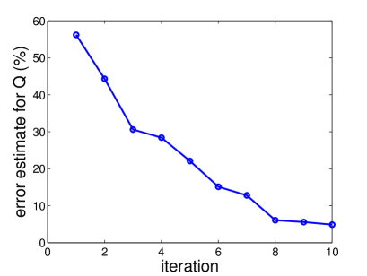
Refer to caption
Figure 40: Flow problem: convergence of the error estimate for Q(uε)𝑄superscript𝑢𝜀Q(u^{\varepsilon}).

7 Conclusions and perspectives

We have introduced efficient numerical tools for the a posteriori error estimation of specific quantities of interest in the context of MsFEM computations. These tools are based on the Constitutive Relation Error concept, that we have previously used in [19] to estimate the error in the energy norm, and that we have here successfully extended to the goal-oriented context.

Our approach leads to fully computable and guaranteed upper bounds on the error, and enables to perform adaptive multiscale computations by selecting the relevant MsFEM parameters to reach a prescribed error tolerance. Our procedure is consistent with the offline/online paradigm of MsFEM, hence yielding affordable additional computational costs.

The performances of the approach have been investigated on several multiscale problems. Fine scale features of the solution are adaptively recovered during the iterations, if and where needed. In particular, the fine-scale features of the solution in some parts of the physical domain may not affect the quantity of interest, and our procedure then prevents the discretization approach to capture them, thus achieving a significant computational gain at no loss in accuracy. Our method thus outperforms the standard a posteriori error estimation strategy (which assesses and controls the error in the energy norm): for an equal tolerance on the error, a coarser discretization is obtained, leading to a smaller computational cost.

Acknowledgements

We thank C. Le Bris for stimulating discussions on the topics addressed in this article. LC thanks Inria for enabling his two-year leave (2014–2016) in the MATHERIALS project team. The work of FL is partially supported by ONR under grant N00014-15-1-2777 and by EOARD under grant FA9550-17-1-0294.

Références

  • [1] Abdulle A., Nonnenmacher A. A posteriori error analysis of the heterogeneous multiscale method for homogenization problems. C.R. Acad. Sci. Paris, Série I 2009; 347:1081–1086.
  • [2] Abdulle A., Nonnenmacher A. A posteriori error estimates in quantities of interest for the finite element heterogeneous multiscale method. Numerical Methods for Partial Differential Equations 2013; 29(5):1629–1656.
  • [3] Ainsworth M., Oden J.T. A posteriori error estimation in finite element analysis. John Wiley & Sons 2000.
  • [4] Akbari Rahimabadi A., Kerfriden P., Bordas S. Scale selection in nonlinear fracture mechanics of heterogeneous materials. Philosophical Magazine 2015; 95(28-30):3328–3347.
  • [5] Allaire G., Brizzi R. A multiscale finite element method for numerical homogenization. SIAM Multiscale Modeling & Simulation 2006; 4(3):790–812.
  • [6] Becker R., Rannacher R. A feed-back approach to error control in finite element methods: Basic analysis and examples. East-West Journal of Numerical Mathematics 1996; 4:237–264.
  • [7] Becker R., Rannacher R. An optimal control approach to shape a posteriori error estimation in finite element methods. Acta Numerica, Cambridge University Press, 2001; 10:1–120.
  • [8] Ben Dhia H., Rateau G. Mathematical analysis of the mixed Arlequin method. C.R. Acad. Sci. Paris 2001; 332(7):649–654.
  • [9] Bensoussan A., Lions J.-L., Papanicolaou G. Asymptotic Analysis for Periodic Structures. Studies in Mathematics and its Applications, vol. 5, North-Holland, Amsterdam, New York 1978.
  • [10] Blanc X., Le Bris C., Lions P.-L. A possible homogenization approach for the numerical simulation of periodic microstructures with defects. Milan Journal of Mathematics 2012; 80(2):351–367.
  • [11] Blanc X., Le Bris C., Lions P.-L. Local profiles and elliptic problems at different scales with defects. C.R. Acad. Sci. Paris, Série I 2015; 353:203–208.
  • [12] Blanc X., Le Bris C., Lions P.-L. Local profiles for elliptic problems at different scales: defects in, and interfaces between periodic structures. Communications in Partial Differential Equations 2015; 40(12):2173–2236.
  • [13] Blanc X., Le Bris C., Lions P.-L., On correctors for linear elliptic homogenization in the presence of local defects. Communications in Partial Differential Equations 2018; 43(6):965–997.
  • [14] Blanc X., Le Bris C., Lions P.-L., On correctors for linear elliptic homogenization in the presence of local defects: the case of advection-diffusion. Journal de Mathématiques Pures et Appliquées 2019; 124:106–122.
  • [15] Brezzi F., Lions J.-L., Pironneau O. Analysis of a chimera method. C.R. Acad. Sci. Paris 2001; 332:655–660.
  • [16] Cao T., Kelly D.W. Pointwise and local error estimates for the quantities of interest in two-dimensional elasticity. Computers and Mathematics with Applications 2003; 46(1):69–79.
  • [17] Chamoin L., Ladevèze P. A non-intrusive method for the calculation of strict and efficient bounds of calculated outputs of interest in linear viscoelasticity problems. Computer Methods in Applied Mechanics and Engineering 2008; 197(9-12):994–1014.
  • [18] Chamoin L., Legoll F. A pedagogical view on a posteriori error estimation in finite element analysis. in preparation.
  • [19] Chamoin L., Legoll F. A posteriori error estimation and adaptive strategy for the control of MsFEM computations. Computer Methods in Applied Mechanics and Engineering 2018; 336:1–38.
  • [20] Chung E.T., Leung W.T., Pollock S. Goal-oriented adaptivity for GMsFEM. Journal of Computational and Applied Mathematics 2016; 296:625–637.
  • [21] Cirak F., Ramm E. A posteriori error estimation and adaptivity for linear elasticity using the reciprocal theorem. Computer Methods in Applied Mechanics and Engineering 1998; 156:351–362.
  • [22] E W., Engquist B., Huang Z. Heterogeneous multiscale method: a general methodology for multiscale modeling. Physical Review B 2003; 67(9):092101.
  • [23] Efendiev Y., Galvis J., Hou T. Generalized multiscale finite element methods. Journal of Computational Physics 2013; 251:116–135.
  • [24] Efendiev Y., Hou T. Multiscale Finite Element Methods: Theory and Applications. Springer, New York 2009.
  • [25] Efendiev Y., Hou T., Wu X.H. Convergence of a nonconforming multiscale finite element method. SIAM Journal of Numerical Analysis 2000; 37(3):888–910.
  • [26] Feyel F. A multilevel finite element method (FE2) to describe the response of highly non-linear structures using generalized continua. Computer Methods in Applied Mechanics and Engineering 2003; 192:3233–3244.
  • [27] Fraeijs de Veubeke B., Hugge M.A. Dual analysis for heat conduction problems by finite elements. International Journal for Numerical Methods in Engineering 1972; 5(1):65–82.
  • [28] Gendre L., Allix O., Gosselet P., Comte F. Non-intrusive and exact global/local techniques for structural problems with local plasticity. Computational Mechanics 2009; 44(2):233–245.
  • [29] Giles M.B., Suli E. Adjoint methods for PDEs: a posteriori error analysis and postprocessing by duality. Acta Numerica 2002:145–236.
  • [30] Grätsch T., Hartmann F. Finite element recovery techniques for local quantities of linear problems using fundamental solutions. Computational Mechanics 2003; 33:15–21.
  • [31] Henning P., Ohlberger M., Schweizer B. An adaptive multiscale finite element method. SIAM Multiscale Modeling & Simulation 2014; 12(3):1078–1107.
  • [32] Hesthaven J., Zhang S., Zhu X. High-order multiscale finite element method for elliptic problems. SIAM Multiscale Modeling & Simulation 2014; 12(2):650–666.
  • [33] Hou T., Wu X.H. A multiscale finite element method for elliptic problems in composite materials and porous media. Journal of Computational Physics 1997; 134:169–189.
  • [34] Hou T., Wu X.H., Cai Z. Convergence of a multiscale finite element method for elliptic problems with rapidly oscillating coefficients. Mathematics of Computation 1999; 68(227):913–943.
  • [35] Hou T., Wu X.H., Zhang Y. Removing the cell resonance error in the multiscale finite element method via a Petrov-Galerkin formulation. Communications in Mathematical Sciences 2004; 2:185–205.
  • [36] Hughes T.J.R., Feijoo G.R., Mazzei L., Quincy J.B. The variational multiscale method – A paradigm for computational mechanics. Computer Methods in Applied Mechanics and Engineering 1998; 166(1-2):3–24.
  • [37] Jhurani C., Demkowicz L. Multiscale modeling using goal-oriented adaptivity and numerical homogenization. Part 1: mathematical formulation and numerical results. Computer Methods in Applied Mechanics and Engineering 2012; 213-216:399–417.
  • [38] Ladevèze P. Strict upper error bounds for calculated outputs of interest in computational structural mechanics. Computational Mechanics 2008; 42(2):271–286.
  • [39] Ladevèze P., Chamoin L. Calculation of strict error bounds for finite element approximations of nonlinear pointwise quantities of interest. International Journal for Numerical Methods in Engineering 2010; 84:1638–1664.
  • [40] Ladevèze P., Leguillon D. Error estimate procedure in the finite element method and applications. SIAM Journal of Numerical Analysis 1983; 20(3):485–509.
  • [41] Ladevèze P., Maunder E.A.W. A general method for recovering equilibrating element tractions. Computer Methods in Applied Mechanics and Engineering 1996; 137:111–151.
  • [42] Ladevèze P., Pelle J.-P. Mastering Calculations in Linear and Nonlinear Mechanics. Springer, 2004.
  • [43] Ladevèze P., Pled F., Chamoin L. New bounding techniques for goal-oriented error estimation applied to linear problems. International Journal for Numerical Methods in Engineering 2013; 93(13):1345–1380.
  • [44] Larson M.G., Malqvist A. Adaptive variational multiscale methods based on a posteriori error estimation: duality techniques for elliptic problems. In B. Engquist, P. Lötstedt, and O. Runborg, editors, Multiscale Methods in Science and Engineering, volume 44 of Lecture Notes in Computational Science and Engineering, pages 181–193. Springer, 2005.
  • [45] Larson M.G., Malqvist A. Adaptive variational multiscale methods based on a posteriori error estimation: energy norm estimates for elliptic problems. Computer Methods in Applied Mechanics and Engineering 2007; 196(21-24):2313–2324.
  • [46] Le Bris C., Legoll F., Lozinski A. An MsFEM type approach for perforated domains. SIAM Multiscale Modeling & Simulation 2014; 12(3):1046–1077.
  • [47] Le Bris C., Legoll F., Thomines F. Multiscale finite element approach for “weakly” random problems and related issues. Mathematical Modelling and Numerical Analysis 2014; 48(3):815–858.
  • [48] Lions J.-L., Pironneau O. Domain decomposition methods for CAD. C.R. Acad. Sci. Paris, Série I 1999; 328(1):73–80.
  • [49] Lozinski A., Pironneau O. Numerical zoom for localized multiscales. Numerical Methods for Partial Differential Equations 2011; 27:197–207.
  • [50] Maier M., Rannacher R. Duality-based adaptivity in finite element discretization of heterogeneous multiscale problems. Journal of Numerical Mathematics 2016; 24(3):167–187.
  • [51] Malqvist A., Peterseim D. Localization of elliptic multiscale problems. Mathematics of Computation 2014; 83(290):2583–2603.
  • [52] Nolen J., Papanicolaou G., Pironneau O. A framework for adaptive multiscale methods for elliptic problems. SIAM Multiscale Modeling & Simulation 2008; 7(1):171–196.
  • [53] Oden J.T., Prudhomme S. Goal-oriented error estimation and adaptivity for the finite element method. Computers and Mathematics with Applications 2001; 41:735–756.
  • [54] Oden J.T., Prudhomme S. Estimation of modeling error in Computational Mechanics. Journal of Computational Physics 2002; 182:496–515.
  • [55] Oden J.T., Reddy J.N. On dual complementary variational principles in mathematical physics. International Journal of Engineering Science 1974; 12:1–29.
  • [56] Oden J.T., Vemaganti K. Estimation of local modeling error and goal-oriented modeling of heterogeneous materials; Part 1: Error estimates and adaptive algorithms. Journal of Computational Physics 2000; 164:22-47.
  • [57] Oden J.T., Vemaganti K., Moës N. Hierarchical modeling of heterogeneous solids. Computer Methods in Applied Mechanics and Engineering 1999; 172(1-4):3–25.
  • [58] Panetier J., Ladevèze P., Chamoin L. Strict and effective bounds in goal-oriented error estimation applied to fracture mechanics problems solved with XFEM. International Journal for Numerical Methods in Engineering 2010; 81:671–700.
  • [59] Paraschivoiu M., Peraire J., Patera A.T. A posteriori finite element bounds for linear functional outputs of elliptic partial differential equations. Computer Methods in Applied Mechanics and Engineering 1997; 150:289–312.
  • [60] Pled F., Chamoin L., Ladevèze P. On the techniques for constructing admissible stress fields in model verification: performances on engineering examples. International Journal for Numerical Methods in Engineering 2011; 88(5):409–441.
  • [61] Prudhomme S., Chamoin L., Ben Dhia H., Bauman P.T. An adaptive strategy for the control of modeling error in two-dimensional atomic-to-continuum coupling simulations. Computer Methods in Applied Mechanics and Engineering 2009; 198(21-26):1887–1901.
  • [62] Prudhomme S., Oden J.T. On goal-oriented error estimation for elliptic problems: application to the control of pointwise errors. Computer Methods in Applied Mechanics and Engineering 1999; 176:313–331.
  • [63] Rannacher R., Suttmeier F.T. A feedback approach to error control in finite element methods: application to linear elasticity. Computational Mechanics 1997; 19:434–446.
  • [64] Strouboulis T., Copps K., Babuska I. The generalized finite element method. Computer Methods in Applied Mechanics and Engineering 2001; 190:4081–4193.
  • [65] Strouboulis T., Zhang L., Wang D., Babuska I. A posteriori error estimation for generalized finite element methods. Computer Methods in Applied Mechanics and Engineering 2006; 195:852–879.
  • [66] Vemaganti K., Oden J.T. Estimation of local modeling error and goal-oriented modeling of heterogeneous materials; Part 2: A computational environment for adaptive modeling of heterogeneous elastic solids. Computer Methods in Applied Mechanics and Engineering 2001; 190:6089-6124.
  • [67] Verfürth R. A review of a posteriori error estimates and adaptive mesh-refinement techniques. Wiley-Teubner 1996.
  • [68] Waeytens J., Chamoin L., Ladevèze P. Guaranteed error bounds on pointwise quantities of interest for transient viscodynamics problems. Computational Mechanics 2012; 49:291–307.