Central Similarity Quantization for Efficient Image and Video Retrieval

Abstract

Existing data-dependent hashing methods usually learn hash functions from pairwise or triplet data relationships, which only capture the data similarity locally, and often suffer from low learning efficiency and low collision rate. In this work, we propose a new global similarity metric, termed as central similarity, with which the hash codes of similar data pairs are encouraged to approach a common center and those for dissimilar pairs to converge to different centers, to improve hash learning efficiency and retrieval accuracy. We principally formulate the computation of the proposed central similarity metric by introducing a new concept, i.e., hash center that refers to a set of data points scattered in the Hamming space with a sufficient mutual distance between each other. We then provide an efficient method to construct well separated hash centers by leveraging the Hadamard matrix and Bernoulli distributions. Finally, we propose the Central Similarity Quantization (CSQ) that optimizes the central similarity between data points w.r.t. their hash centers instead of optimizing the local similarity. CSQ is generic and applicable to both image and video hashing scenarios. Extensive experiments on large-scale image and video retrieval tasks demonstrate that CSQ can generate cohesive hash codes for similar data pairs and dispersed hash codes for dissimilar pairs, achieving a noticeable boost in retrieval performance, i.e. 3%-20% in mAP over the previous state-of-the-arts

.

1 Introduction

(a) Doublet(pairwise)

(b) Triplet

(c) Central similarity

Figure 1: The intuition behind pairwise/triplet similarity based hashing methods and the proposed center similarity quantization. Pairwise and triplet learnings only consider a pair/triplet of data at once, while our central similarity encourages all similar data points to collapse to the corresponding hash centers (red stars).

(a) Doublet (pairwise similarity)

(b) Triplet (triplet similarity)

(c) HashNet

(d) Central similarity (ours)

Figure 2: Visualization of hash codes generated by four deep hash learning methods using different data similarity metrics, trained on MNIST with ten groups of data points (one class for a group). The first two methods use pairwise and triplet similarity respectively. HashNet [2] adopts weighted pairwise similarity.

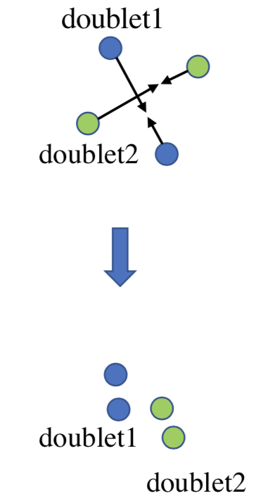
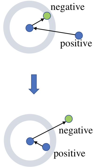
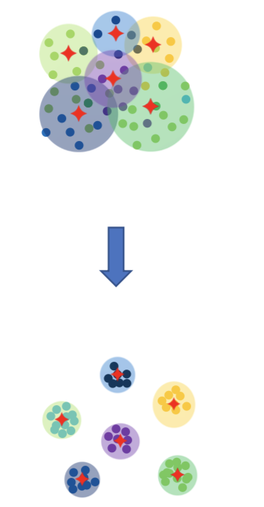
By transforming high-dimensional data to compact binary hash codes in the Hamming space via a proper hash function [37], hashing offers remarkable efficiency for data storage and retrieval. Recently, “deep learning to hash” methods [14, 32, 21, 18, 22, 44] have been successfully applied to large-scale image retrieval [44, 48] and video retrieval [8, 28, 21], which can naturally represent a nonlinear hash function for producing hash codes of input data.

Most deep hashing methods [2, 48, 27, 18] learn hash functions by utilizing pairwise or triplet data similarity, where the data relationships are captured from a local perspective. Such pairwise/triplet based hash learning intrinsically leads to the following issues. 1) Low-efficiency in profiling similarity among the whole training dataset. The commonly used pairwise similarity [2, 48, 18] or triplet similarity metrics [27, 14] have a time complexity at an order of $\mathcal{O}(n!)$ for $n$ data points. Thus, it is impractical to exhaustively learn from all the possible data pairs/triplets for large-scale image or video data. 2) Insufficient coverage of data distribution. Pairwise/triplet similarity based methods utilize only partial relationships between data pairs, which may harm the discriminability of the generated hash codes. 3) Low effectiveness on imbalanced data. In real-world scenarios, the number of dissimilar pairs is much larger than that of similar pairs. Hence, pairwise/triplet similarity based hashing methods cannot learn similarity relationships adequately to generate sufficiently good hash codes, leading to restricted performance.

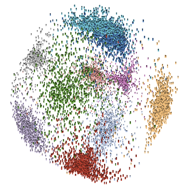
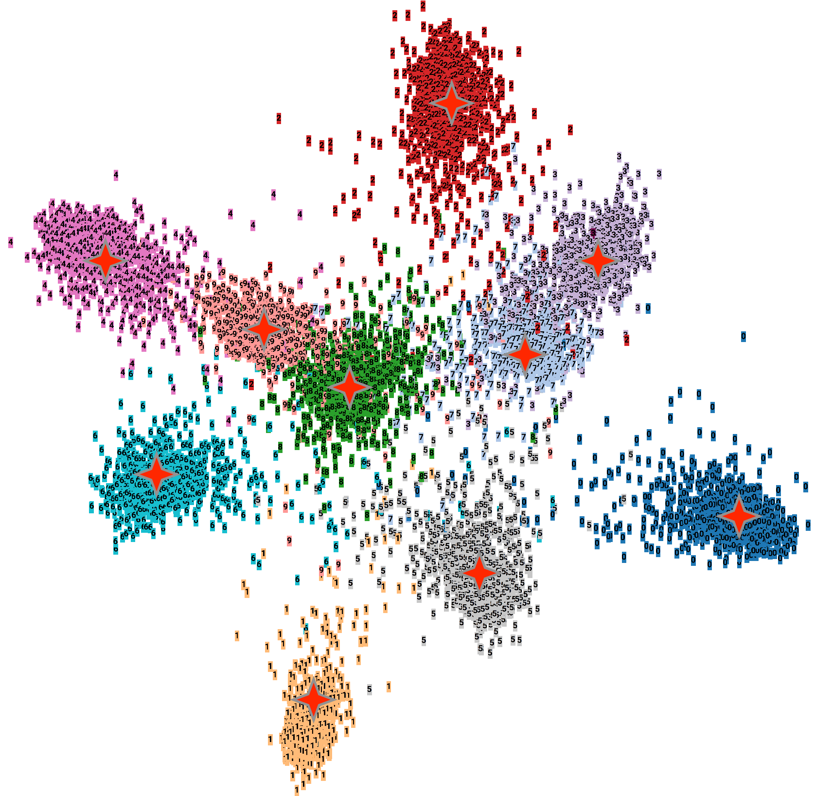
To address the above issues, we propose a new global similarity metric, termed as central similarity, which we optimize constantly for obtaining better hash functions. Specifically, the central similarity measures Hamming distances between hash codes and the hash center which is defined as a set of points in the Hamming space with a sufficient mutual distance. Central similarity learning aims at encouraging the generated hash codes to approach the corresponding hash center. With a time complexity of only $\mathcal{O}(nm)$ for $n$ data points and $m$ centers, central similarity based hashing is highly efficient and can generate discriminative enough hash codes from the global data distribution (Fig. 1), which overcomes the limitations of hashing methods based on the pairwise/triplet similarity. Even in the presence of severe data imbalance, the hash functions can still be well learned from global relationships.

To obtain suitable hash centers, we propose two systematic approaches. One is to directly construct hash centers with maximal mutual Hamming distance by leveraging the Hadamard matrix; the other is to generate hash centers by randomly sampling from Bernoulli distributions. We prove that both approaches can generate proper hash centers that are separated from each other with a sufficient Hamming distance. We also consider jointly learning hash centers from data with hash functions. However, we empirically find that learned centers by some common methods [11, 43, 29] cannot provide better hash functions than the analytically constructed ones. We present comparisons on the hash centers from different methods in Sec. 4.5.

With the generated hash centers, we develop the central similarity with Convolutional Neural Networks (CNNs), to learn a deep hash function in the Hamming space. We name the proposed hashes learning approach as Central Similarity Quantization (CSQ). In particular, we adopt convolutional layers for learning data features and a hash layer for yielding hash codes. After identifying the hash centers, we train the deep CNN and the hash layer end-to-end to generate hash codes with the goal of optimizing central similarity. CSQ is generic and applicable to learning hash codes for both images and videos.

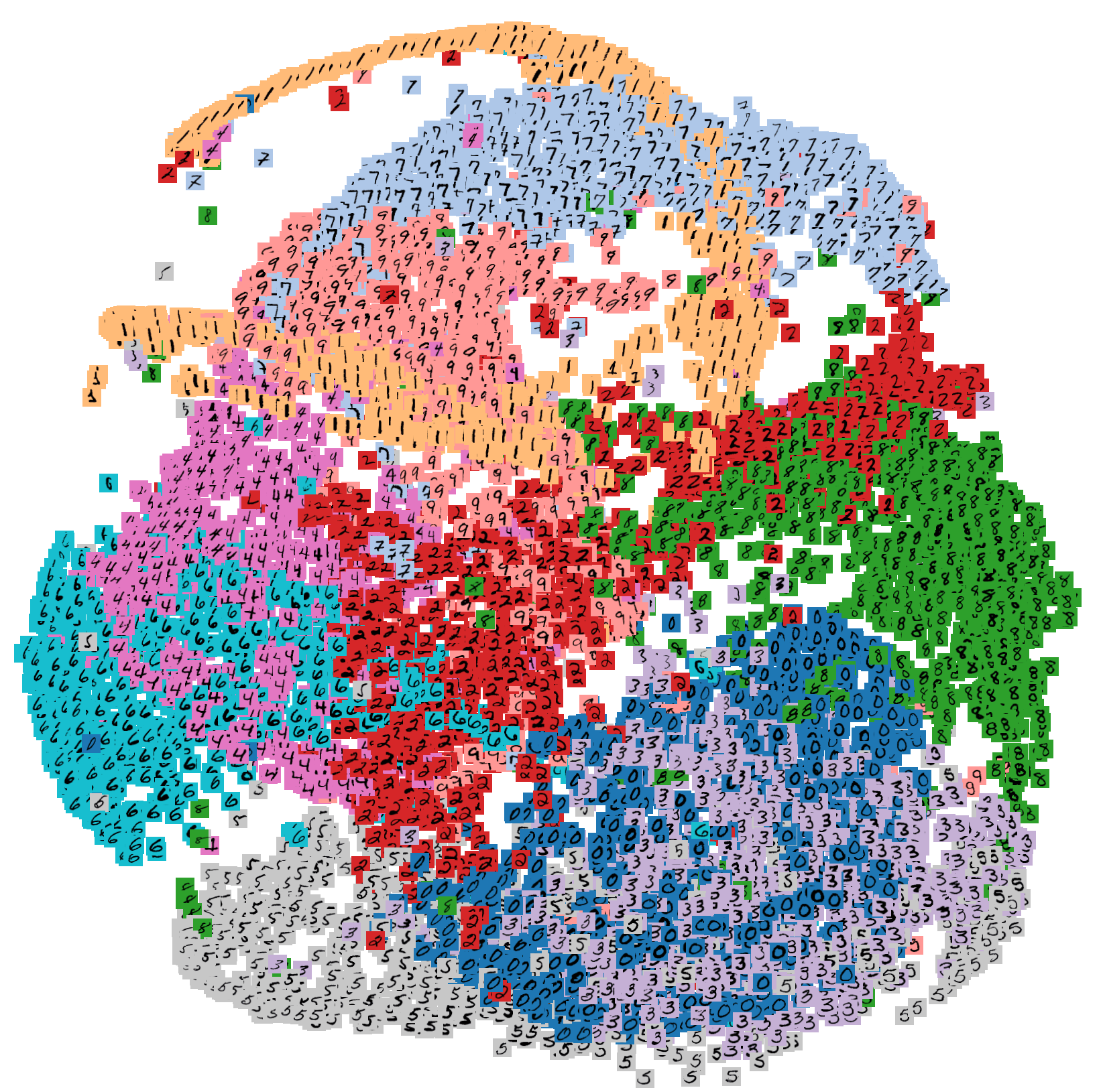
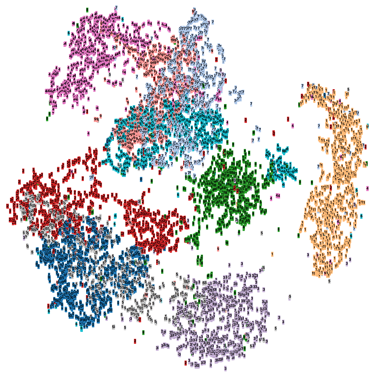
We conduct illustrative experiments on MNIST [15] at first to validate the effectiveness of our CSQ. We find that the hash codes learned by CSQ show favorable intra-class compactness and inter-class separability compared with other state-of-the-art hashing methods, as shown in Fig. 2. Then we perform extensive comparative experiments on three benchmark datasets for image hashing and two video datasets for video hashing respectively. With CSQ, noticeable improvements in retrieval performance are achieved, i.e., 3%-20% in mAP, also with a 3 to 5.5 $\times$ faster training speed over the latest methods.

Our contributions are three-fold. 1) We rethink data similarity modeling and propose a novel concept of hash center for capturing data relationships more effectively. We present two systematic methods to generate proper hash centers rapidly. 2) We introduce a novel central similarity based hashing method. It can capture the global data distribution and generate high-quality hash functions efficiently. To our best knowledge, this is the first work to utilize global similarity and hash centers for deep hash function learning. 3) We present a deep learning model to implement our method for both image and video retrieval and establish new state-of-the-arts.

2 Related Work

The “deep learning to hash” methods such as CNNH [44], DNNH [14], DHN [48], DCH [1] and HashNet [2] have been successfully applied to image hashing. They adopt 2D CNNs to learn image features and then use hash layers to learn hash codes. Recent hashing methods for images focus on how to design a more efficient pairwise-similarity loss function. DNNH [14] proposes to use a triplet ranking loss for similarity learning. DHN [48] uses Maximum a Posterior (mAP) estimation to obtain the pairwise similarity loss function. HashNet [2] adopts the Weighted Maximum Likelihood (WML) estimation to alleviate the severe the data imbalance by adding weights in pairwise loss functions. Different from previous works [41, 25, 23, 26, 38, 31, 32, 19, 34, 16, 17, 45], this work proposes a new central similarity metric and use it to model the relationships between similar and dissimilar pairs for improving the discriminability of generated hash codes.

Compared with image analysis, video analysis aims to utilize the temporal information [33, 6, 39, 36, 3, 47, 46]. Video hashing methods such as DH [28], SRH [8], DVH [21] exploit the temporal information in videos compared with image hashing. For instance, [28] utilizes Disaggregation Hashing to exploit the correlations among different feature dimensions. [8] presents an LSTM-based method to capture the temporal information between video frames. Recently, [21] fuses the temporal information by using fully-connected layers and frame pooling. Different from these hashing methods, our proposed CSQ is a generic method for both image and video hashing. Through directly replacing 2D CNNs with 3D CNNs, the proposed CSQ can well capture the temporal information for video hashing.

Our CSQ is partially related to center loss in face recognition [43] which uses a center loss to learn more discriminative representation for face recognition (classification). The centers in [43] are derived from the feature representation of the corresponding categories, which are unstable with intra-class variations. Different from this center loss for recognition [43], our proposed hash center is defined over hash codes instead of feature representations, and can help generate high-quality hash codes in the Hamming space.

3 Method

We consider learning a hash function in a supervised manner from a training set of $N$ data points $\mathcal{X}=\left\{\{x_{i}\}_{i=1}^{N}\,,\,L\right\}$, where each $x_{i}\in\mathbb{R}^{D}$ is a data point to hash and $L$ denotes the semantic label set for data $\mathcal{X}$. Let $f:x\mapsto h\in\left\{0,1\right\}^{K}$ denote the nonlinear hash function from the input space $\mathbb{R}^{D}$ to $K$-bit Hamming space $\left\{0,1\right\}^{K}$. Similar to other supervised “deep learning to hash” methods [2, 48], we pursue a hash function that is able to generate hash codes $h$’s for the data points $x$’s which are close in the Hamming space and share similar semantic labels.

We define a set of points $\mathcal{C}=\{c_{1},c_{2},\ldots,c_{m}\}\subset\{0,1\}^{K}$ with a sufficient distance in the Hamming space as hash centers, and propose to learn hash functions supervised by the central similarity w.r.t. $\mathcal{C}$. The central similarity would encourage similar data pairs to be close to a common hash center and dissimilar data pairs to be distributed around different hash centers respectively. Through such central similarity learning, the global similarity information between data pairs can be preserved in $f$, yielding high-quality hash codes.

In below, we first give a formal definition of hash center and explain how to generate proper hash centers systematically. Then we elaborate on the details of the central similarity quantization.

3.1 Definition of Hash Center

The most intuitive motivation is to learn hash centers from image or video features, such that the learned centers preserve “distinctness” between different data points. However, we find that hash centers learned from data features with diverse mutual Hamming distance do not perform better than hash centers with pre-defined Hamming distance (in Experiments, Sec 4.5). We thus assume that each center should be more distant from the other centers than to the hash codes associated with it. As such, the dissimilar pairs can be better separated and similar pairs can be aggregated cohesively. Based on the observation and intuition, we formally define a set of points in the Hamming space as valid hash centers with the following properties.

Definition 1 (Hash Center).

We define hash centers as a set of points $\mathcal{C}=\left\{c_{i}\right\}_{i=1}^{m}\subset\left\{0,1\right\}^{K}$ in the $K$-dimensional Hamming space with an average pairwise distance satisfying

$$\frac{1}{T}\sum_{i\neq j}^{m}D_{H}\left(c_{i},c_{j}\right)\geqslant\frac{K}{2},$$ (1)

where $D_{H}$ is the Hamming distance, $m$ is the number of hash centers, and $T$ is the number of combinations of different $c_{i}$ and $c_{j}\in\mathcal{C}$.

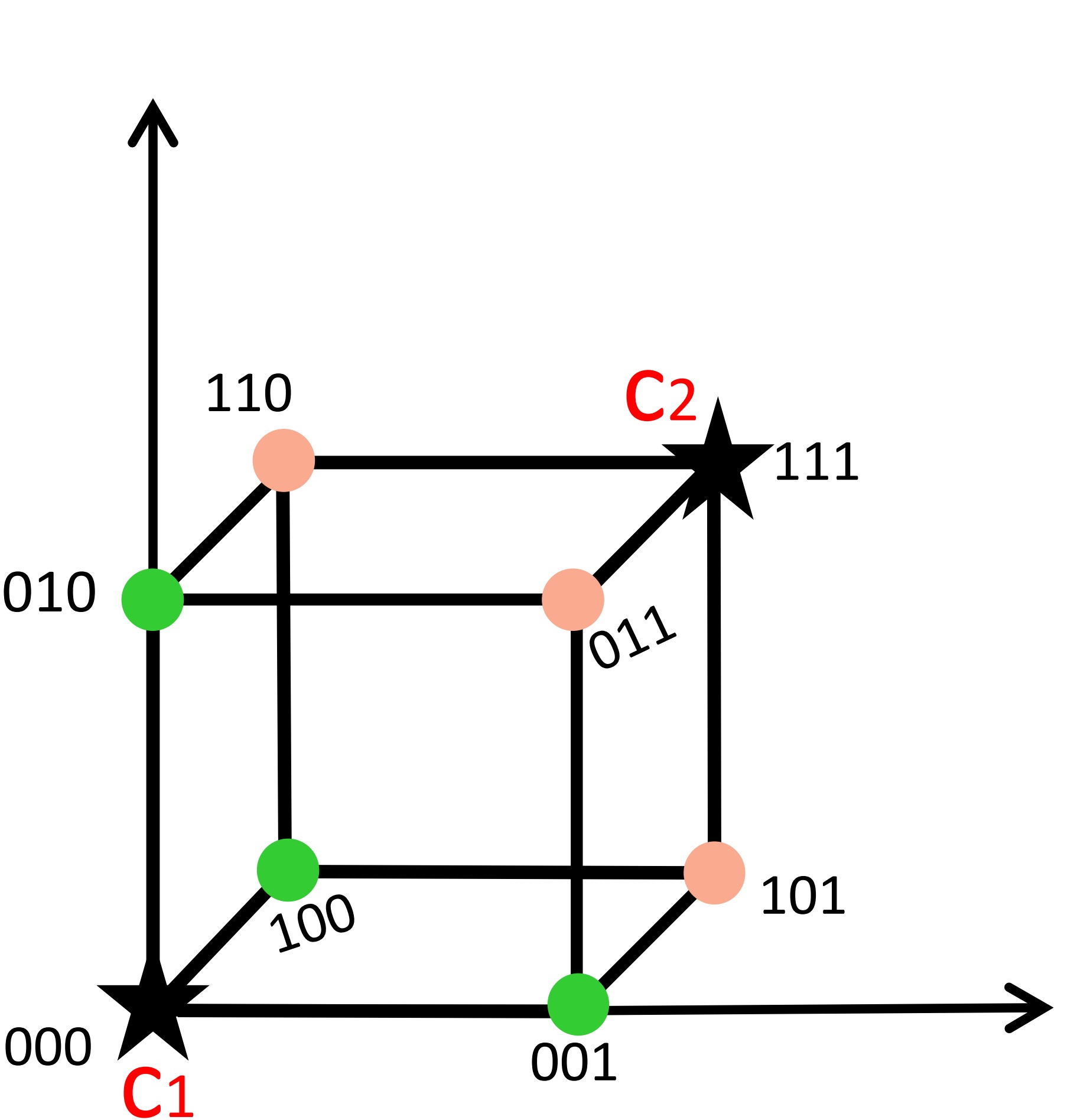
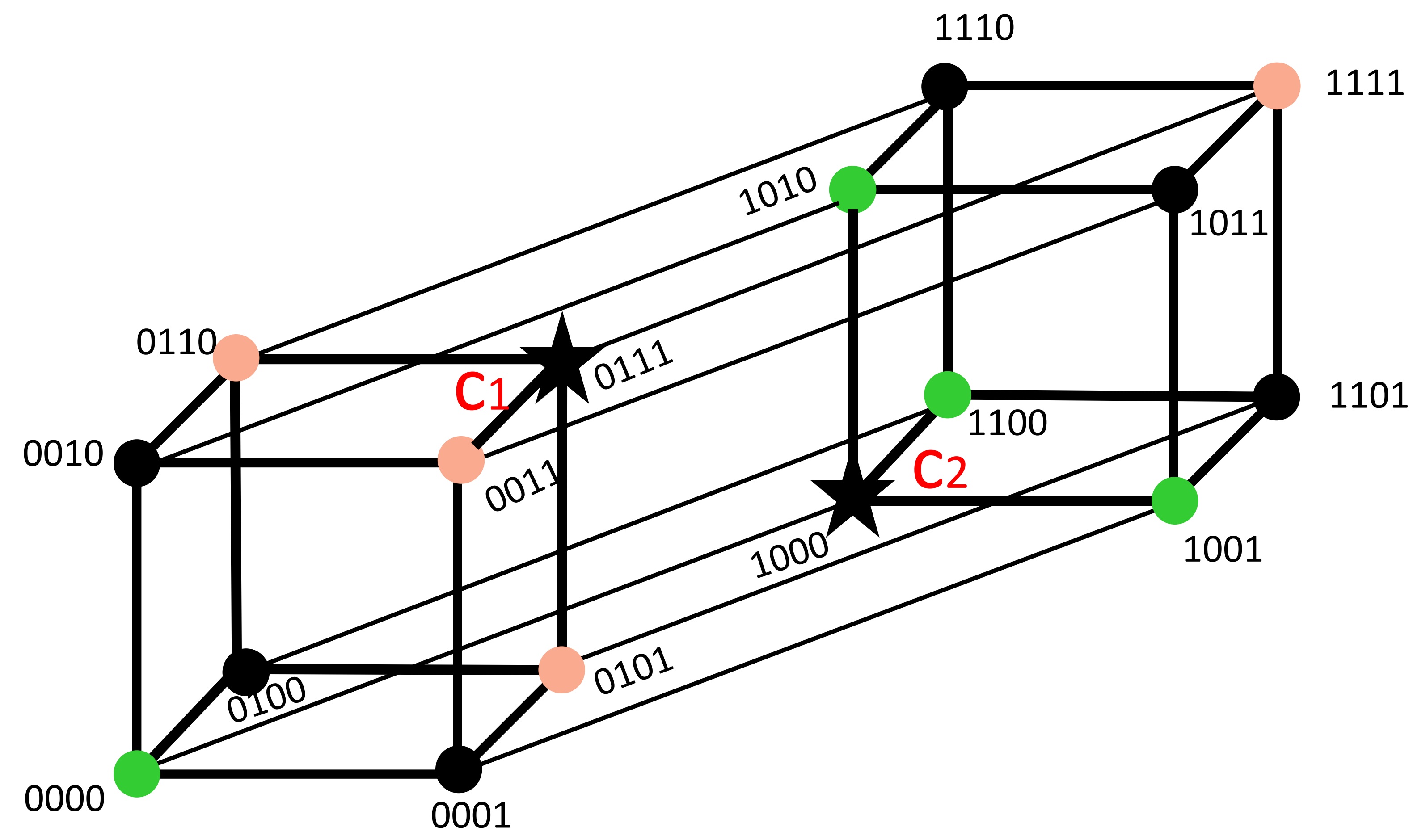
For better clarity, we show some examples of the desired hash centers in the 3d and 4d Hamming spaces in Fig. 3. In Fig. 3(a), the hash center of hash codes $[0,1,0]$, $[0,0,1]$ and $[1,0,0]$ is $c_{1}$, and the Hamming distance between $c_{1}$ and $c_{2}$ is 3. In Fig. 3(b), we use a 4d hypercube to represent the 4d Hamming spaces. The two stars $c_{1}$ and $c_{2}$ are the hash centers given in Definition 1. The distance between $c_{1}$ and $c_{2}$ is $D_{H}\left(c_{1},c_{2}\right)=4$, and the distance between the green dots and the center $c_{2}$ is the same ($D_{H}=1$). However, we do not strictly require all points to have the same distance from the corresponding center. Instead, we define the nearest center as the corresponding hash center for a hash code.

(a) 3d Hamming space

(b) 4d Hamming space

Figure 3: The illustration of hash centers in 3d and 4d Hamming spaces.

3.2 Generation of Hash Centers

We develop two approaches for generating valid hash centers based on the following observation. In the $K$-dimensional Hamming space (throughout this paper, $K$ is set to an even number), if a set of points are mutually orthogonal, they will have an equal distance of $K/2$ to each other. Namely, they are valid hash centers satisfying Definition 1.

Our first approach is to generate hash centers by leveraging the following nice properties of a Hadamard matrix. It is known that a $K\times K$ Hadamard matrix $H_{K}=[h_{a}^{1};\ldots;h_{a}^{K}]$ satisfies: 1) It is a squared matrix with rows $h_{a}^{i}$ being mutually orthogonal, i.e., the inner products of any two row vectors $\langle h_{a}^{i},h_{a}^{j}\rangle=0$. The Hamming distance between any two row vectors is $D_{H}(h_{a}^{i},h_{a}^{j})=\frac{1}{2}(K-\langle h_{a}^{i},h_{a}^{j}\rangle)={K}/{2}$. Therefore, we can choose hash centers from these row vectors. 2) Its size $K$ is a power of $2$ (i.e., $K=2^{n}$), which is consistent with the customary number of bits of hash codes. 3) It is a binary matrix whose entries are either -1 or +1. We can simply replace all -1 with 0 to obtain hash centers in $\left\{0,1\right\}^{K}$.

To sample the hash centers from the Hadamard matrix, we first build a $K\times K$ Hadamard matrix by Sylvester’s construction [42] as follows:

$$\centering H_{K}=\begin{bmatrix}H_{2^{n-1}}&H_{2^{n-1}}\\ H_{2^{n-1}}&-H_{2^{n-1}}\end{bmatrix}=H_{2}\otimes H_{2^{n-1}},\@add@centering$$ (2)

where $\otimes$ represents the Hadamard product, and $K=2^{n}$. The two factors within the initial Hadamard matrix are $H_{1}=\begin{bmatrix}1\end{bmatrix}$ and $H_{2}=\begin{bmatrix}1&1\\ 1&-1\end{bmatrix}$. When the number of centers $m\leqslant K$, we directly choose each row to be a hash center. When $K<m\leqslant 2K$, we use a combination of two Hadamard matrices $H_{2K}=[H_{K},-H_{K}]^{\top}$ to construct hash centers.

Input : The number of hash centers $m$, the dimension of the Hamming space (hash codes) $K$.

Initialization: construct a $K\times K$ Hadamard matrix $H_{K}=\left[h_{a}^{i}\right]$ and construct $H_{2K}=[H_{K},-H_{K}]^{\top}=\left[h_{2k}^{i}\right].$

for iteration $i$, $i{=}1$ to $m$ do

       if $m\leqslant K$ & $K=2^{n}$ then   //   $n$ is any $\mathbb{Z}^{+}$

            $c_{i}=h_{a}^{i}$;

       end if

      else if $K<m\leqslant 2K$ & $K=2^{n}$  then

            $c_{i}=h_{2k}^{i}$;

       else

             $c_{i}[\text{random half position}]=1$;

             $c_{i}[\text{other half position}]=0$;

       end if

      

end for

Replace all -1 with 0 in these centers;

Output : hash centers: $\mathcal{C}=\left\{c_{1},\ldots,c_{m}\right\}\subset\{0,1\}^{K}$.

Algorithm 1 Generation of Hash Centers

Though applicable in most cases, the number of valid centers generated by the above approach is constrained by the fact that the Hadamard matrix is a squared one. If $m$ is larger than $2K$ or $K$ is not the power of 2, the first approach is inapplicable. We thus propose the second generation approach by randomly sampling the bits of each center vector. In particular, each bit of a center $c_{i}$ is sampled from a Bernoulli distribution $\mathrm{Bern(0.5)}$ where $P(x=0)=0.5$ if $x\sim\mathrm{Bern(0.5)}$. We can easily prove that the distance between these centers is $K/2$ in expectation. Namely, $\mathbb{E}[D_{H}(c_{i},c_{j})]=K/2$ if $c_{i},c_{j}\sim\mathrm{Bern(0.5)}$. We summarize these two approaches in Alg. 1. The generation algorithm is very efficient and only needs a trivial computation/time cost to generate hash centers.

Once a set of hash centers is obtained, the next step is to associate the training data samples $\mathcal{X}$ with their individual corresponding centers to compute the central similarity. Recall $L$ is the semantic label for $\mathcal{X}$, and usually $L=\{l_{1},\ldots,l_{q}\}$. For single-label data, each data sample belongs to one category, while each multi-label data sample belongs to more than one category. We term the hash centers that are generated from Alg. 1 and associated with semantic labels as semantic hash centers. We now explain how to obtain the semantic hash centers for single- and multi-label data separately.

Semantic hash centers for single-label data

For single-label data, we assign one hash center for each category. That is, we generate $q$ hash centers $\{c_{1},\ldots,c_{q}\}$ by Alg. 1 corresponding to labels $\{l_{1},\ldots,l_{q}\}$. Thus, data pairs with the same label share a common center and are encouraged to be close to each other. Because each data sample is assigned to one hash center, we obtain the semantic hash centers $\mathcal{C^{\prime}}=\{c^{\prime}_{1},c^{\prime}_{2},\ldots,c^{\prime}_{N}\}$, where $c^{\prime}_{i}$ is the hash center of $x_{i}$.

Semantic hash centers for multi-label data

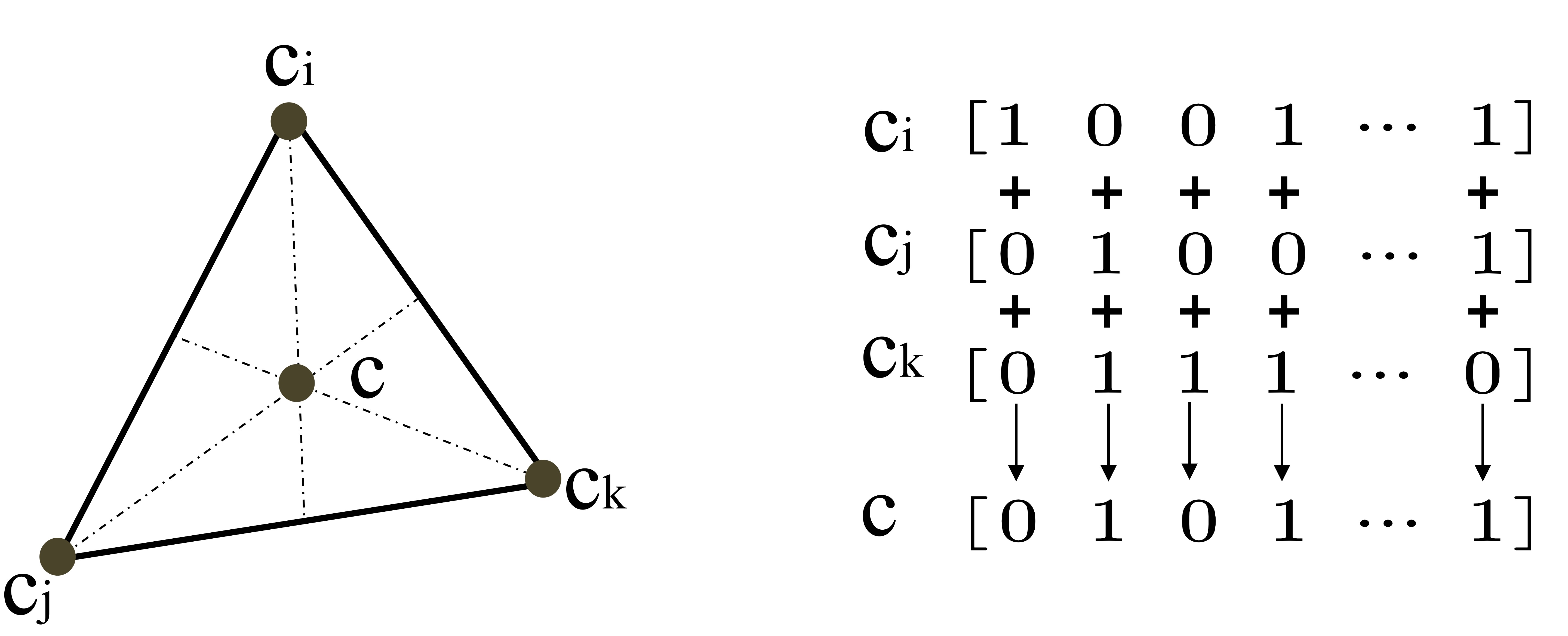
For multi-label data, DCH [1], HashNet [2] and DHN [48] directly make data pairs similar if they share at least one category. However, they ignore the transitive similarity when data pairs share more than one category. In this paper, we generate transitive centers for data pairs sharing multiple labels. First, we generate $q$ hash centers $\{c_{1},\ldots,c_{q}\}$ by Alg. 1 corresponding to semantic labels $\{l_{1},\ldots,l_{q}\}$. Then for data including two or more categories, we calculate the centroid of these centers, each of which corresponds to a single category. For example, suppose one data sample $x\in\mathcal{X}$ has three categories $l_{i}$, $l_{j}$ and $l_{k}$. The centers of the three categories are $c_{i}$, $c_{j}$ and $c_{k}$, as shown in Fig. 4. We calculate the centroid $c$ of the three centers as the hash center of $x$. To ensure the elements to be binary, we calculate each bit by voting at the same bit of the three centers and taking the value that dominates, as shown in the right panel of Fig. 4. If the number of 0 is equal to the number of 1 at some bits (i.e., the voting result is a draw), we sample from $\mathrm{Bern(0.5)}$ for these bits. Finally, for each $x_{i}\in\mathcal{X}$, we take the centroid as its semantic hash center, and then obtain semantic hash centers $\mathcal{C^{\prime}}=\{c^{\prime}_{1},c^{\prime}_{2},\ldots,c^{\prime}_{N}\}$, where $c^{\prime}_{i}$ is the hash center of $x_{i}$.

Figure 4: Semantic hash center for multi-label data.

3.3 Central Similarity Quantization

Given the generated centers $\mathcal{C}=\{c_{1},\ldots,c_{q}\}$ for training data $\mathcal{X}$ with $q$ categories, we obtain the semantic hash centers $\mathcal{C^{\prime}}=\{c^{\prime}_{1},c^{\prime}_{2},\ldots,c^{\prime}_{N}\}$ for single- or multi-label data, where $c^{\prime}_{i}$ denotes the hash center of the data sample $x_{i}$. We derive the central similarity learning objective by maximizing the logarithm posterior of the hash codes w.r.t. the semantic hash centers. Formally, the logarithm Maximum a Posterior (MAP) estimation of hash codes $\mathcal{H}=\left[h_{1},...,h_{N}\right]$ for all the training data can be obtained by maximizing the following likelihood probability:

$$\log P(\mathcal{H}|\mathcal{C^{\prime}})\propto\log P(\mathcal{C^{\prime}}|\mathcal{H})P(\mathcal{H})=\sum_{i}^{N}\log P(c^{\prime}_{i}|h_{i})P(h_{i}),\vspace{-10pt}$$

where $P(\mathcal{H})$ is the prior distribution over hash codes and $P(\mathcal{C^{\prime}}|\mathcal{H})$ is the likelihood function. $P(c^{\prime}_{i}|h_{i})$ is the conditional probability of center $c^{\prime}_{i}$ given hash code $h_{i}$. We model $P(\mathcal{C^{\prime}}|\mathcal{H})$ as a Gibbs distribution: $P(c^{\prime}_{i}|h_{i})=\frac{1}{\alpha}\exp(-\beta D_{H}(c^{\prime}_{i},h_{i}))$, where $\alpha$ and $\beta$ are constants, and $D_{H}$ measures the Hamming distance between a hash code and its hash center. Since hash centers are binary vectors, we use Binary Cross Entropy (BCE) to measure the Hamming distance between the hash code and its center, $D_{H}(c^{\prime}_{i},h_{i})=\text{BCE}(c^{\prime}_{i},h_{i})$. So the conditional probability is calculated as $\log P(c^{\prime}_{i}|h_{i})\propto-\frac{1}{K}\sum_{k\in K}(c^{\prime}_{i,k}\log h_{i,k}+(1-c^{\prime}_{i,k})\log(1-h_{i,k}))$. We can see that the larger the conditional probability $P(c^{\prime}_{i}|h_{i})$ is, the smaller the Hamming distance will be between hash code $h$ and its hash center $c$, implying that the hash code is close to its corresponding center; otherwise the hash code is far away from its corresponding center. By substituting $\log P(c^{\prime}_{i}|h_{i})$ into the MAP estimation, we obtain the optimization objective of the central similarity loss $L_{C}$:

$$L_{C}= \frac{1}{K}\sum_{i}^{N}\sum_{k\in K}\left[c^{\prime}_{i,k}\log h_{i,k}+(1-c^{\prime}_{i,k})\log(1-h_{i,k})\right].$$ (3)

Since each hash center is binary, existing optimization cannot guarantee that the generated hash codes completely converge to hash centers [40] due to the inherent optimization difficulty. So we introduce a quantization loss $L_{Q}$ to refine the generated hash codes $h_{i}$. Similar to DHN [48], we use the bi-modal Laplacian prior for quantization, which is defined as $L_{Q}=\sum_{i\neq j}^{N}(|||2h_{i}-\textbf{1}|-\textbf{1}||_{1})$, where $\textbf{1}\in\mathbb{R}^{K}$ is an all-one vector. As $L_{Q}$ is a non-smooth function which makes it difficult to calculate its derivative, we adopt the smooth function $\log\cosh$ [10] to replace it. So $|x|\approx\log\cosh x$. Then the quantization loss $L_{Q}$ becomes

$$L_{Q}= \sum_{i}^{N}\sum_{k=1}^{K}(\log\cosh(|2h_{i,k}-1|-1).$$ (4)

Finally, we have central similarity optimization problem:

$$\min_{\Theta}L_{T}=L_{C}+\lambda_{1}L_{Q}\vspace{-5pt}$$ (5)

where $\Theta$ is the set of all parameters for deep hash function learning, and $\lambda_{1}$ is the hyper-parameter obtained through grid search in our work.

Based on the loss function $L_{T}$, we adopt the standard framework [9, 2] in deep-hashing methods to conduct CSQ. Specifically, multiple convolutional layers are adopted to learn data features and a hash layer with three $fc$ layers and ReLU as the activation function is used to generate hash codes. The detailed framework of CSQ is given in the supplementary material.

4 Experiments

We conduct experiments for both image and video retrieval to evaluate our CSQ against several state-of-the-arts. Five benchmark (image and video) datasets are used in our experiments and their statistics are summarized in Tab. 1.

Table 1: Experimental settings for all datasets. DI (Data Imbalance) is ratio between the number of dissimilar and similar pairs.

Dataset	Data Type	#Train	#Test	#Retrieval	DI
ImageNet	image	10,000	5,000	128,495	100:1
MS COCO	image	10,000	5,000	112,217	1:1
NUS_WIDE	image	10,000	2,040	149,685	5:1
UCF101	video	9.5k	3.8k	9.5k	101:1
HMDB51	video	3.5k	1.5k	3.5k	51:1

Table 2: Comparison in mAP of Hamming Ranking for different bits on image retrieval.

Method	ImageNet (mAP@1000)			MS COCO (mAP@5000)			NUS-WIDE (mAP@5000)
	16 bits	32 bits	64 bits	16 bits	32 bits	64 bits	16 bits	32 bits	64 bits
ITQ-CCA [7]	0.266	0.436	0.576	0.566	0.562	0.502	0.435	0.435	0.435
BRE [13]	0.063	0.253	0.358	0.592	0.622	0.634	0.485	0.525	0.544
KSH [24]	0.160	0.298	0.394	0.521	0.534	0.536	0.394	0.407	0.399
SDH [32]	0.299	0.455	0.585	0.554	0.564	0.580	0.575	0.590	0.613
CNNH [44]	0.315	0.473	0.596	0.599	0.617	0.620	0.655	0.659	0.647
DNNH [14]	0.353	0.522	0.610	0.644	0.651	0.647	0.703	0.738	0.754
DHN [48]	0.367	0.522	0.627	0.719	0.731	0.745	0.712	0.759	0.771
HashNet [2]	0.622	0.701	0.739	0.745	0.773	0.788	0.757	0.775	0.790
DCH [1]	0.652	0.737	0.758	0.759	0.801	0.825	0.773	0.795	0.818
CSQ (Ours)	0.851	0.865	0.873	0.796	0.838	0.861	0.810	0.825	0.839

Table 3: Comparison in mAP of Hamming Ranking by adopting different backbones (AlexNet or ResNet50) to learn features.

Method	ImageNet (AlexNet)			ImageNet (ResNet50)
	16 bits	32 bits	64 bits	16 bits	32 bits	64 bits
CNNH [44]	0.282	0.453	0.548	0.315	0.473	0.596
DNNH [14]	0.303	0.457	0.572	0.353	0.522	0.610
DHN [48]	0.318	0.473	0.569	0.367	0.522	0.627
HashNet [2]	0.506	0.631	0.684	0.622	0.701	0.739
DCH [1]	0.529	0.637	0.664	0.652	0.737	0.758
CSQ (Ours)	0.601	0.653	0.695	0.851	0.865	0.873

Table 4: Training time (in mins) comparison on three datasets with different hash bits.(One GPU: TITAN X; Backbone: AlexNet).

Method	ImageNet		COCO		NUS_WIDE
	32 bits	64 bits	32 bits	64 bits	32 bits	64 bits
DHN [48]	3.87e2	4.13e2	3.92e2	4.05e2	3.56e2	3.63e2
HashNet [2]	6.51e2	6.84e2	6.42e2	6.88e2	7.29e2	7.34e2
CSQ (Ours)	0.92e2	1.01e2	1.13e2	1.15e2	1.30e2	1.39e2

4.1 Experiments on Image Hashing

Datasets

We use three image benchmark datasets, including ImageNet [30], NUS_WIDE [5] and MS COCO [20]. On ImageNet, we use the same data and settings as [2, 48]. As ImageNet is a single-label dataset, we directly generate one hash center for each category. MS COCO is a multi-label image dataset with 80 categories. NUS_WIDE is also a multi-label image dataset, and we choose images from the 21 most frequent categories for evaluation [48, 14]. For MS COCO and NUS_WIDE datasets, we first generate 80 and 21 hash centers for all categories respectively, and then calculate the centroid of the multi-centers as the semantic hash centers for each image with multiple labels, following the approach in Sec. 3.2. The visualization of generated hash centers is given in the supplementary material.

Baselines and evaluation metrics

We compare retrieval performance of our proposed CSQ with nine classical or state-of-the-art hashing/quantization methods, including four supervised shallow methods ITQ-CCA [7], BRE [13], KSH [24], SDH [32] and five supervised deep methods CNNH [44], DNNH [14], DHN [48], HashNet [2] and DCH [1]. For the four shallow hashing methods, we adopt the results from the latest works [48, 2, 1] to make them directly comparable. We evaluate image retrieval performance based on four standard evaluation metrics: Mean Average Precision (mAP), Precision-Recall curves (PR), and Precision curves w.r.t. different numbers of returned samples (P@N), Precision curves within Hamming distance 2 (P@H=2). We adopt mAP@1000 for ImageNet as each category has 1,300 images, and adopt mAP@5000 for MS COCO and NUS_WIDE.

(a) P-R curve @64bits

(b) P@N @64bits

(c) P@H=2

Figure 5: Experimental results of CSQ and compared methods on ImageNet w.r.t. three evaluation metrics.

(a) P-R curve @64bits

(b) P@N @64bits

(c) P@H=2

Figure 6: Experimental results of CSQ and compared methods on UCF101 w.r.t. three evaluation metrics.

Results

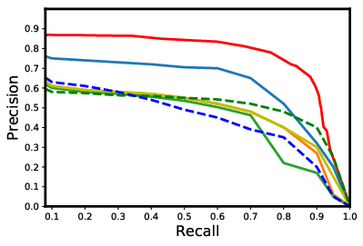
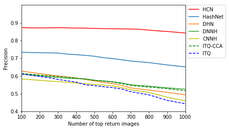
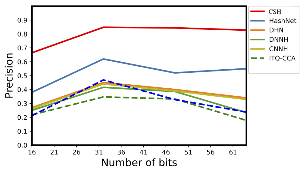
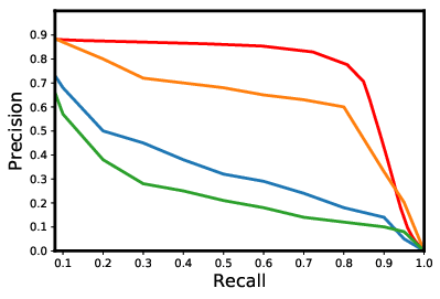
Results in terms of Mean Average Precision (mAP) for image retrieval are given in Tab. 2 and 3. In Tab. 2, we take ResNet50 as the backbone for CNNH, DNNH, DHN, HashNet, DCH and our CSQ. In Tab. 3, we take AlexNet and ResNet50 as backbone respectively for five deep methods and our CSQ. From Tab. 2, we can observe that our CSQ achieves the best performance on the image retrieval task. Compared with the state-of-the-art deep hashing methods HashNet and DCH, our CSQ brings an increase of at least 11.5%, 3.6%, 3.1% in mAP for different bits on ImageNet, MS COCO and NUS_WIDE, respectively. And some retrieval performance boost up to 20%. Specifically, the mAP boost on ImageNet is much larger than that on the other two datasets, i.e., about 7%-9%. Note that ImageNet has the most severe data imbalance among the three image retrieval datasets (Tab. 1). From Tab. 3, we can observe that our method achieves superior performance by adopting both AlexNet and ResNet50 as backbone architectures. Fig. 5 shows the retrieval performance in Precision-Recall curves (P-R curve), Precision curves w.r.t. different numbers of returned samples (P@N) and Precision curves with Hamming distance 2(P@H=2) respectively on ImageNet. We can find CSQ outperforms all compared methods by large margins on ImageNet w.r.t. the three performance metrics. Additionally, we compare the training time in Tab. 4 and the proposed CSQ achieves a 3 to 5.5 $\times$ faster training speed over DHN and HashNet.

4.2 Experiments on Video Hashing

Datasets

Two video retrieval datasets, UCF101 [35] and HMDB51 [12], are used with their default settings. On UCF101, we use 9.5k videos for training and retrieval, and 3.8k queries in every split. For HMDB51, we have 3.5k videos for training and retrieval, and 1.5k videos for testing (queries) in each split.

Baselines

We compare the retrieval performance of the proposed CSQ against three supervised deep video hashing methods: DH [28], DLSTM [49] and SRH [8] based on the same evaluation metrics as image retrieval experiments.

Results

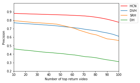
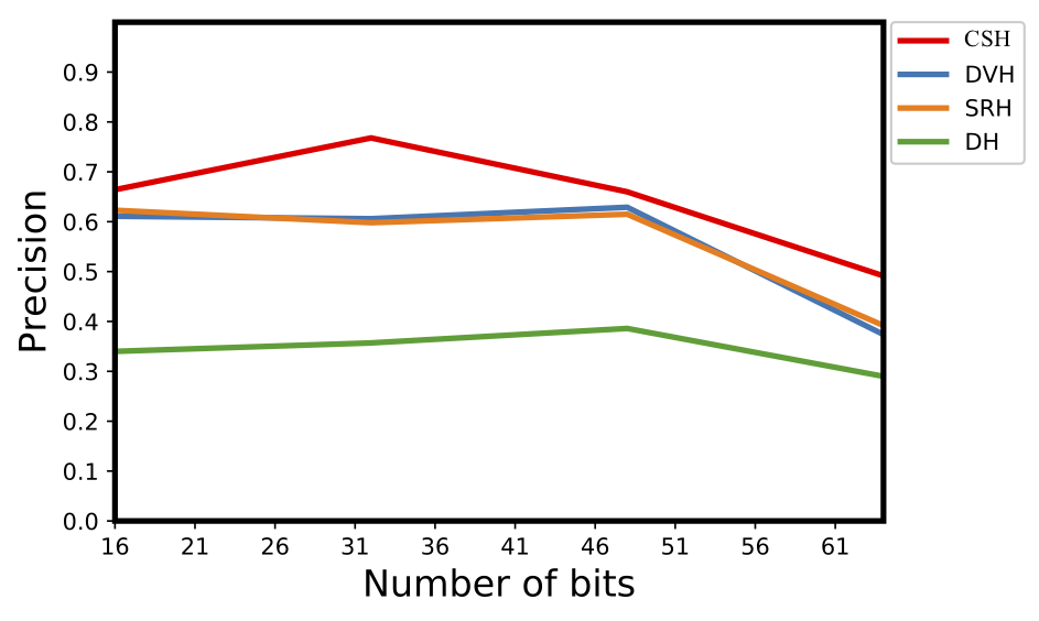
In Tab. 5, our CSQ also achieves significant performance boost on video retrieval. It achieves impressive mAP increases of over 12.0% and 4.8% for different bits on UCF101 and HMDB51, respectively. The larger improvements by our method on UCF101 are mainly due to its severe data imbalance. Fig. 6 shows the retrieval performance in Precision-Recall curves (P-R curve), Precision curves w.r.t. different numbers of returned samples (P@N) and Precision curves with Hamming distance 2(P@H=2) respectively on UCF101. From the figure, we can observe that CSQ also outperforms all compared methods by large margins on UCF101 w.r.t. the three performance metrics. In a nutshell, the proposed CSQ performs consistently well under different evaluation metrics.

Table 5: Comparison in mAP of Hamming Ranking for different bits on video retrieval.

Method	UCF-101 (mAP@100)			HMDB51 (mAP@70)
	16 bits	32 bits	64 bits	16 bits	32 bits	64 bits
DH [28]	0.300	0.290	0.470	0.360	0.360	0.310
SRH [8]	0.716	0.692	0.754	0.491	0.503	0.509
DVH [21]	0.701	0.705	0.712	0.441	0.456	0.518
CSQ (Ours)	0.838	0.875	0.874	0.527	0.565	0.579

Differences from image hashing

For video hashing, we need to obtain temporal information by replacing 2D CNN with 3D CNN. In our experiments, CSQ adopts a lightweight 3D CNN, Multi-Fiber 3D CNN [4], as the convolutional layers to learn the features of videos. And the hash layers keep unchanged.

4.3 Visualization

Visualization of retrieved results

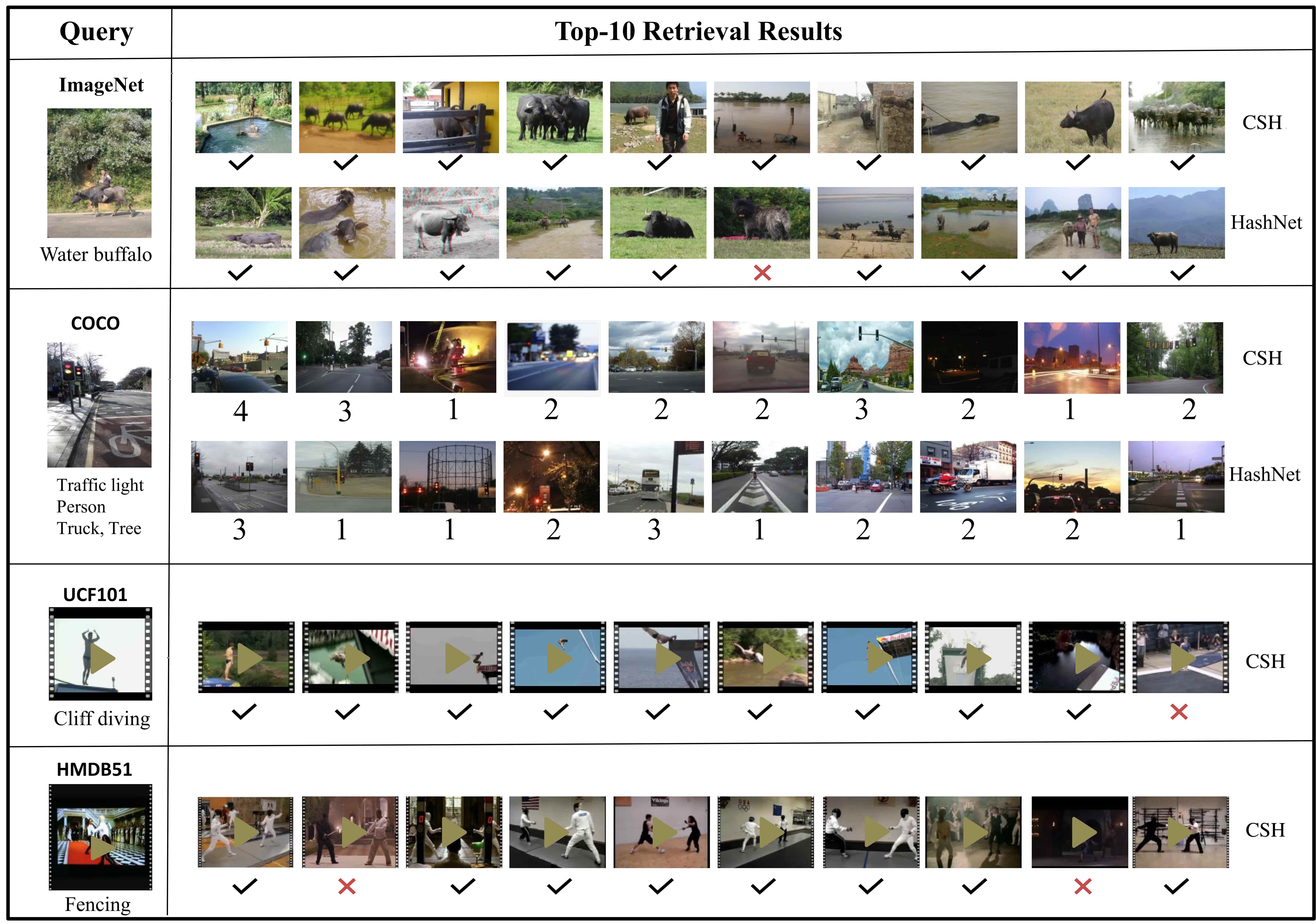
We show the retrieval results on ImageNet, MS COCO, UCF101 and HMDB51 in Fig. 7. It can be seen that CSQ can return much more relevant results. On MS COCO, CSQ uses the centroid of multiple centers as the hashing target for multi-label data, so the returned images of CSQ share more common labels with the query compared with HashNet.

Figure 7: Examples of top 10 retrieved images and videos for two image datasets and two video datasets. For COCO images, below each image the number of common labels with the query is given.

Visualization of hash code distance

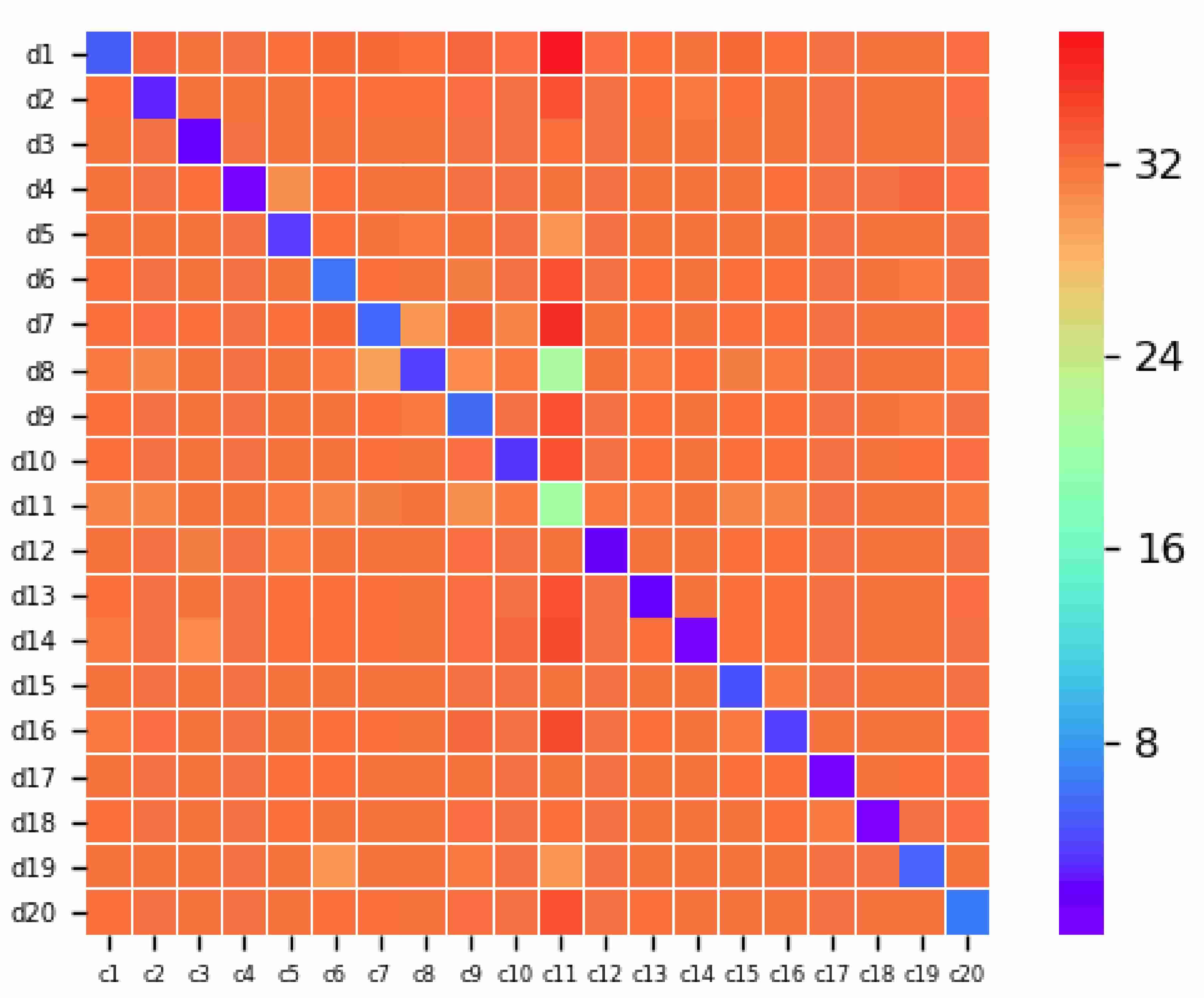
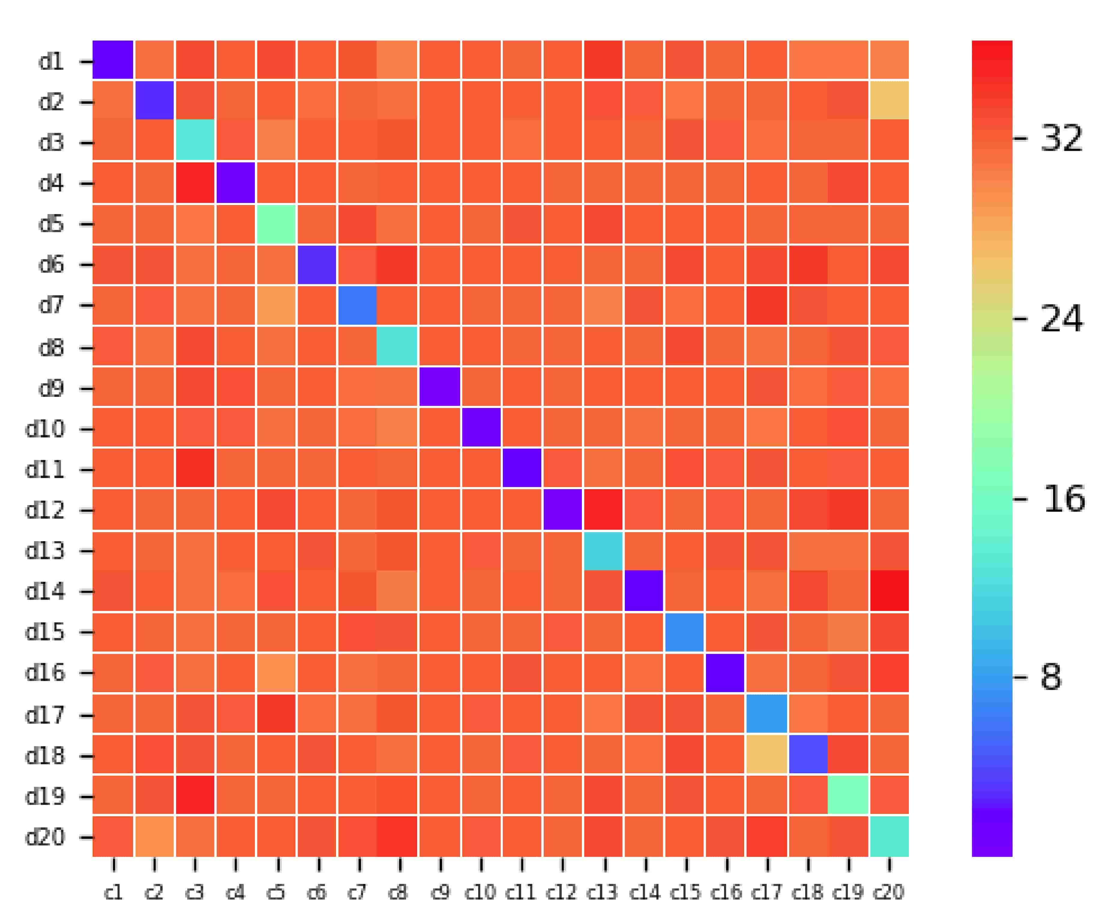
We visualize the Hamming distance between 20 hash centers and generated hash codes of ImageNet and UCF101 by heat maps in Fig. 8. The columns represent the 20 hash centers of test data in ImageNet (with 1k test images sampled) or UCF101 (with 0.6k test videos sampled). The rows are the generated hash codes assigned to these 20 centers. We calculate the average Hamming distance between hash centers and hash codes assigned to different centers. The diagonal values in the heat maps are the average Hamming distances of the hash codes with the corresponding hash center. We find that the diagonal values are small, meaning the generated hash codes “collapse” to the corresponding hash centers in the Hamming space. Most off-diagonal values are very large, meaning that dissimilar data pairs spread sufficiently.

(a) ImageNet	(b) UCF101

Figure 8: The heat maps of average Hamming distance between 20 hash centers (the columns) with hash codes (64bit, rows) generated by the proposed CSQ from test data in ImageNet and UCF101.

4.4 Ablation Study

We investigate the effects of the proposed central similarity, traditional pairwise similarity, and quantization process for hash function learning, by evaluating different combinations of central similarity loss $L_{C}$, pairwise similarity loss $L_{P}$, and quantization loss $L_{Q}$. The results are summarized in Tab. 6. Our CSQ includes $L_{C}$ and $L_{Q}$, corresponding to the 1st row in Tab. 6. When we add $L_{P}$ to CSQ (2nd row), mAP only increases for some bits. This shows that pairwise similarity has limited effects on further improving over central similarity learning. We add $L_{P}$ while removing $L_{C}$ (3rd row), and find that the mAP decreases significantly for various bits. When only using $L_{C}$, the mAP just decreases slightly. These results show the positive effects of central similarity learning.

Table 6: The mAP results of CSQ and its three variants on one image dataset and one video dataset.

			ImageNet (mAP@1000)			UCF101 (mAP@100)
$L_{C}$	$L_{P}$	$L_{Q}$	16 bits	32 bits	64 bits	16 bits	32 bits	64 bits
✓		✓	0.851	0.865	0.873	0.838	0.875	0.874
✓	✓	✓	0.847	0.870	0.871	0.840	0.868	0.881
	✓	✓	0.551	0.629	0.655	0.716	0.739	0.784
✓			0.841	0.864	0.870	0.824	0.854	0.867

4.5 Hash Center Learning

In our work, we pre-compute hash centers by using the Hadamard matrix or sampling from a Bernoulli distribution, which is independent of image or video data. We ignore the “distinctness” between any two dissimilar data points. For example, the “distinctness” between dog and cat should be smaller than that between dog and car. A more intuitive method should be to learn centers from image or video features rather than pre-defined hash centers, which can preserve the similarity information between data points in hash centers. Here we adopt three existing methods to learn centers from features and then compare the learned centers with our pre-computed hash centers, to prove the validity of our proposed hash center generation methods. The three methods to be compared are 1) center learning in face recognition (Face Center) [43], 2) center learning in fine-grained classification (Magnet Center) [29], and 3) center learning in Representative-based Metric Learning (RepMet Center) [11]. We give the details of the three types of learned centers in supplementary material, including loss functions, hyper-parameters and quantization loss to binarize centers for hashing. We apply these learned centers to hashing as the method in Sec 3.3 and the retrieval results are given in Tab. 7. We observe the learned centers obtain worse performance than that with our methods. Also, compared with these center learning methods, our pre-computing methods only needs trivial computation/time cost but achieves superior performance. One potential reason is that the fixed hash centers are binary codes while the learned centers are not binary, so we need to do an extra quantization operation on the learned centers, which hurts the similarity information between learned centers and causes worse performances. .

Table 7: Comparison between three learned centers with our hash centers on image and video retrieval.

Method	ImageNet (mAP@1000)			UCF-101 (mAP@100)
	16bits	32bits	64bits	16bits	32bits	64bits
Face Center	0.718	0.723	0.744	0.693	0.745	0.817
Magnet Center	0.758	0.801	0.818	0.715	0.793	0.821
RepMet Center	0.804	0.815	0.827	0.781	0.829	0.835
Our Center	0.851	0.865	0.873	0.838	0.875	0.874

5 Conclusion and Future Work

In this paper, we propose a novel concept “Hash Center” to formulate the central similarity for deep hash learning. The proposed Central Similarity Quantization (CSQ) can learn hash codes by optimizing the Hamming distance between hash codes with corresponding hash centers. It is experimentally validated that CSQ can generate high-quality hash codes and yield state-of-the-art performance for both image and video retrieval. In this work, we generate hash centers independently of data rather than learning from data features, which has been proven effective. In the future, we will continue to explore how to learn better hash centers.

Acknowledgement

This work was supported by AI.SG R-263-000-D97-490, NUS ECRA R-263-000-C87-133 and MOE Tier-II R-263-000-D17-112.

References

- [1] Y. Cao, M. Long, B. Liu, and J. Wang. Deep cauchy hashing for hamming space retrieval. In Proceedings of the IEEE Conference on Computer Vision and Pattern Recognition, pages 1229–1237, 2018.
- [2] Z. Cao, M. Long, J. Wang, and S. Y. Philip. Hashnet: Deep learning to hash by continuation. In ICCV, pages 5609–5618, 2017.
- [3] Y.-W. Chao, S. Vijayanarasimhan, B. Seybold, D. A. Ross, J. Deng, and R. Sukthankar. Rethinking the faster r-cnn architecture for temporal action localization. In Proceedings of the IEEE Conference on Computer Vision and Pattern Recognition, pages 1130–1139, 2018.
- [4] Y. Chen, Y. Kalantidis, J. Li, S. Yan, and J. Feng. Multi-fiber networks for video recognition. arXiv preprint arXiv:1807.11195, 2018.
- [5] T.-S. Chua, J. Tang, R. Hong, H. Li, Z. Luo, and Y. Zheng. Nus-wide: a real-world web image database from national university of singapore. In Proceedings of the ACM international conference on image and video retrieval, page 48. ACM, 2009.
- [6] J. Donahue, L. Anne Hendricks, S. Guadarrama, M. Rohrbach, S. Venugopalan, K. Saenko, and T. Darrell. Long-term recurrent convolutional networks for visual recognition and description. In Proceedings of the IEEE conference on computer vision and pattern recognition, pages 2625–2634, 2015.
- [7] Y. Gong, S. Lazebnik, A. Gordo, and F. Perronnin. Iterative quantization: A procrustean approach to learning binary codes for large-scale image retrieval. IEEE Transactions on Pattern Analysis and Machine Intelligence, 35(12):2916–2929, 2013.
- [8] Y. Gu, C. Ma, and J. Yang. Supervised recurrent hashing for large scale video retrieval. In Proceedings of the 2016 ACM on Multimedia Conference, pages 272–276. ACM, 2016.
- [9] K. He, X. Zhang, S. Ren, and J. Sun. Deep residual learning for image recognition. In Proceedings of the IEEE conference on computer vision and pattern recognition, pages 770–778, 2016.
- [10] A. Hyvärinen, J. Hurri, and P. O. Hoyer. Natural image statistics: a probabilistic approach to early computational vision. Springer.
- [11] L. Karlinsky, J. Shtok, S. Harary, E. Schwartz, A. Aides, R. Feris, R. Giryes, and A. M. Bronstein. Repmet: Representative-based metric learning for classification and few-shot object detection. In Proceedings of the IEEE Conference on Computer Vision and Pattern Recognition, pages 5197–5206, 2019.
- [12] H. Kuehne, H. Jhuang, R. Stiefelhagen, and T. Serre. Hmdb51: A large video database for human motion recognition. In High Performance Computing in Science and Engineering ‘12, pages 571–582. Springer, 2013.
- [13] B. Kulis and T. Darrell. Learning to hash with binary reconstructive embeddings. In Advances in neural information processing systems, pages 1042–1050, 2009.
- [14] H. Lai, Y. Pan, Y. Liu, and S. Yan. Simultaneous feature learning and hash coding with deep neural networks. In Proceedings of the IEEE conference on computer vision and pattern recognition, pages 3270–3278, 2015.
- [15] Y. LeCun. The mnist database of handwritten digits. http://yann. lecun. com/exdb/mnist/, 1998.
- [16] C. Li, C. Deng, N. Li, W. Liu, X. Gao, and D. Tao. Self-supervised adversarial hashing networks for cross-modal retrieval. In Proceedings of the IEEE conference on computer vision and pattern recognition, pages 4242–4251, 2018.
- [17] C. Li, S. Gao, C. Deng, D. Xie, and W. Liu. Cross-modal learning with adversarial samples. In Advances in Neural Information Processing Systems, pages 10791–10801, 2019.
- [18] W.-J. Li, S. Wang, and W.-C. Kang. Feature learning based deep supervised hashing with pairwise labels. arXiv preprint arXiv:1511.03855, 2015.
- [19] Y. Li, W. Liu, and J. Huang. Sub-selective quantization for learning binary codes in large-scale image search. IEEE transactions on pattern analysis and machine intelligence, 40(6):1526–1532, 2017.
- [20] T.-Y. Lin, M. Maire, S. Belongie, J. Hays, P. Perona, D. Ramanan, P. Dollár, and C. L. Zitnick. Microsoft coco: Common objects in context. In European conference on computer vision, pages 740–755. Springer, 2014.
- [21] V. E. Liong, J. Lu, Y.-P. Tan, and J. Zhou. Deep video hashing. IEEE Transactions on Multimedia, 19(6):1209–1219, 2017.
- [22] H. Liu, R. Wang, S. Shan, and X. Chen. Deep supervised hashing for fast image retrieval. In Proceedings of the IEEE conference on computer vision and pattern recognition, pages 2064–2072, 2016.
- [23] W. Liu, C. Mu, S. Kumar, and S.-F. Chang. Discrete graph hashing. In Advances in neural information processing systems, pages 3419–3427, 2014.
- [24] W. Liu, J. Wang, R. Ji, Y.-G. Jiang, and S.-F. Chang. Supervised hashing with kernels. In 2012 IEEE Conference on Computer Vision and Pattern Recognition, pages 2074–2081. IEEE, 2012.
- [25] W. Liu, J. Wang, S. Kumar, and S.-F. Chang. Hashing with graphs. 2011.
- [26] W. Liu and T. Zhang. Multimedia hashing and networking. IEEE MultiMedia, 23(3):75–79, 2016.
- [27] M. Norouzi, D. J. Fleet, and R. R. Salakhutdinov. Hamming distance metric learning. In Advances in neural information processing systems, pages 1061–1069, 2012.
- [28] J. Qin, L. Liu, M. Yu, Y. Wang, and L. Shao. Fast action retrieval from videos via feature disaggregation. Computer Vision and Image Understanding, 156:104–116, 2017.
- [29] O. Rippel, M. Paluri, P. Dollar, and L. Bourdev. Metric learning with adaptive density discrimination. arXiv preprint arXiv:1511.05939, 2015.
- [30] O. Russakovsky, J. Deng, H. Su, J. Krause, S. Satheesh, S. Ma, Z. Huang, A. Karpathy, A. Khosla, M. Bernstein, et al. Imagenet large scale visual recognition challenge. International Journal of Computer Vision, 115(3):211–252, 2015.
- [31] F. Shen, W. Liu, S. Zhang, Y. Yang, and H. Tao Shen. Learning binary codes for maximum inner product search. In Proceedings of the IEEE International Conference on Computer Vision, pages 4148–4156, 2015.
- [32] F. Shen, C. Shen, W. Liu, and H. Tao Shen. Supervised discrete hashing. In Proceedings of the IEEE conference on computer vision and pattern recognition, pages 37–45, 2015.
- [33] K. Simonyan and A. Zisserman. Two-stream convolutional networks for action recognition in videos. In Advances in neural information processing systems, pages 568–576, 2014.
- [34] D. Song, W. Liu, R. Ji, D. A. Meyer, and J. R. Smith. Top rank supervised binary coding for visual search. In Proceedings of the IEEE International Conference on Computer Vision, pages 1922–1930, 2015.
- [35] K. Soomro, A. R. Zamir, and M. Shah. Ucf101: A dataset of 101 human actions classes from videos in the wild. arXiv preprint arXiv:1212.0402, 2012.
- [36] G. Varol, I. Laptev, and C. Schmid. Long-term temporal convolutions for action recognition. IEEE transactions on pattern analysis and machine intelligence, 40(6):1510–1517, 2017.
- [37] J. Wang, W. Liu, S. Kumar, and S.-F. Chang. Learning to hash for indexing big data—a survey. Proceedings of the IEEE, 104(1):34–57, 2016.
- [38] J. Wang, W. Liu, A. X. Sun, and Y.-G. Jiang. Learning hash codes with listwise supervision. In Proceedings of the IEEE International Conference on Computer Vision, pages 3032–3039, 2013.
- [39] L. Wang, Y. Xiong, Z. Wang, Y. Qiao, D. Lin, X. Tang, and L. Van Gool. Temporal segment networks: Towards good practices for deep action recognition. In European conference on computer vision, pages 20–36. Springer, 2016.
- [40] T. Weise, M. Zapf, R. Chiong, and A. J. Nebro. Why is optimization difficult? In Nature-Inspired Algorithms for Optimisation, pages 1–50. Springer, 2009.
- [41] Y. Weiss, A. Torralba, and R. Fergus. Spectral hashing. In Advances in neural information processing systems, pages 1753–1760, 2009.
- [42] E. W. Weisstein. Hadamard matrix. 2002.
- [43] Y. Wen, K. Zhang, Z. Li, and Y. Qiao. A discriminative feature learning approach for deep face recognition. In European Conference on Computer Vision, pages 499–515. Springer, 2016.
- [44] R. Xia, Y. Pan, H. Lai, C. Liu, and S. Yan. Supervised hashing for image retrieval via image representation learning. In AAAI, volume 1, page 2, 2014.
- [45] E. Yang, T. Liu, C. Deng, W. Liu, and D. Tao. Distillhash: Unsupervised deep hashing by distilling data pairs. In Proceedings of the IEEE Conference on Computer Vision and Pattern Recognition, pages 2946–2955, 2019.
- [46] L. Yuan, E. H. F. Tay, P. Li, and J. Feng. Unsupervised video summarization with cycle-consistent adversarial lstm networks. IEEE Transactions on Multimedia, 2019.
- [47] L. Yuan, F. E. Tay, P. Li, L. Zhou, and J. Feng. Cycle-sum: cycle-consistent adversarial lstm networks for unsupervised video summarization. In Proceedings of the AAAI Conference on Artificial Intelligence, volume 33, pages 9143–9150, 2019.
- [48] H. Zhu, M. Long, J. Wang, and Y. Cao. Deep hashing network for efficient similarity retrieval. In AAAI, pages 2415–2421, 2016.
- [49] N. Zhuang, J. Ye, and K. A. Hua. Dlstm approach to video modeling with hashing for large-scale video retrieval. In Pattern Recognition (ICPR), 2016 23rd International Conference on, pages 3222–3227. IEEE, 2016.