A Shallow Water Model for Water Flow on Vegetated Hillslope

Abstract

The hillslope hydrological processes are very important in watershed hydrology research. In this paper we focus on the water flow over the soil surface with vegetation in a hydrographic basin. We introduce a PDE model based on general principles of fluid mechanics where the unknowns are water depth and water velocity. The influence of the plant cover to the water dynamics is given by porosity (a quantity related to the density of the vegetation), which is a function defined over the hydrological basin. Using finite volume method for approximating the spatial derivatives, we build an ODE system which constitutes the base of the discrete model we will work with. We discuss and investigate several physical relevant properties of this model. Finally, we perform different quantitative validation tests by comparing numerical results with exact solutions or with laboratory measured data. We also consider some qualitative validation tests by numerically simulating the flow on a theoretical vegetated soil and on a real hydrographic basin.
Keywords: hydrological process, non-homogeneous hyperbolic system, shallow water equations, finite volume method, well-balanced scheme, porosity
2010 MSC: 35L03, 35L60, 35Q35, 65M08, 74F10.

1 Introduction

The mathematical modeling of hydrodynamic processes in hydrographic basins is a challenging subject. There are two main difficulties: the complexity of the phenomena and the multitude of the factors involved in the process. However, there are plenty of performant models dedicated to some specific aspects of the hydrodynamic processes only. To review the existent mathematical models is beyond the purposes of this paper, but we can group them into two large classes: physical base models and regression models. The most known regression models are the unit hydrograph [12] and universal soil loss [43, 50]. From the first class, we mention here a few well known models: SWAT [47], SWAP [46] and KINEROS [51]. Due to the complexity and heterogeneity of the processes (see [38]), models in this class are not purely physical because they need additional empirical relations. The main difference between models here is given by the nature of the empirical relations. For example, in order to model the surface of the water flow, SWAP and KINEROS use a mass balance equation and a closure relation, while SWAT combines the mass balance equation with the momentum balance equation. A very special class of models are cellular automata which combine microscale physical laws with empirical closure relations in a specific way to build up a macroscale model, e.g. CAESAR [8, 24]. In this paper, we introduce a model that extends the shallow water equations and takes into account the presence of vegetation on the soil surface. Such kind of extension is not new; we remind here some applications that use similar models: flow through rigid vegetation [32], flash food propagation in the urban area [18, 19] and tsunami advance in the coastal region [48]. Our model results as an asymptotic limit of a space averaged version of the mass conservation equation and linear momentum balance equations [27, 28]. It takes into account the plant vegetation density, water-plant interaction, soil topography and water-soil interaction. One note that if the cover plant is uniform distributed on the soil, there are not variations in the plant type and plant density, the model reduces to the classical shallow water equation. For numerical applications, we introduce a discrete version of the model. First, we use a finite volume method to discretize the space variable and space derivatives. The resulting ordinary differential system of equations sets up the base of the full discrete model. Then, we introduce a fractional time step scheme to discretize the time variable and time derivatives appearing in the ODE model. Since water flow is the main driving force in more complex phenomena like soil erosion or pollutant spreading, one needs a water flow modulus to be easily incorporated in a large computational package. For this reason, we develop a simple discrete model with low algebraic calculations and reduced memory requirements. For a coupled model water flow - soil erosion and for the influence of the emergent vegetation on soil erosion, the reader is referred to [22] and [2], respectively.

Acknowledging that there must be a balance between the accuracy of the model and the computational cost of it, we underline that we will focus on a first order numerical method dedicated especially to practical applications on the field. This option is a compromise between the precision of the measured data on the field and the accuracy of the method. High order schemes require higher computing resources and can become prohibitive (due to the enormous increase of the volume of processed data) when they are applied at the natural scale of hydrographic basins.

In Section 2 we introduce the PDE model; the reader is referred to [27, 28] for more details concerning this model. Section 3 is dedicated to the numerical approximation of the solution for this model. Section 3.1 deals with the FVM space discretization of the continuum PDE model. The method is described in some details to facilitate a less familiar reader with the FVM method to understand the discrete version of the continuum model and to allow him to develop a proper approximation scheme. In Section 3.2 we investigate some physical relevant qualitative properties of this ODE system: monotonicity of the energy, positivity of the water depth function $h$ and well-balanced properties of the scheme. In Section 3.3 we obtain the full discrete version of our continuous model. In fact, this last version provides the numerical result of the model.

Section 4 is devoted to the validation of the numerical method and the continuum PDE model. Section 4.1 deals with the internal validation. To analyze the performance of the numerical scheme, we compare the numerical results with the exact solutions of PDE in three cases: flow over a bump, the Tacker solution and the solution of the Riemann problem of the shallow water equations. The solutions of Riemann problem of the shallow water equation with topography and vegetation require a deep discussion. If in the case of the shallow water equation without topography and vegetation there is no doubt concerning the solution of the problem, in the case of shallow water equations with topography and vegetation the definition of solution of the problem require new concepts, measure solution and path connection, [10, 25]. When we compare a numerical solution with a theoretical one, there are two relevant aspects for us: the dependence of the theoretical solution on the definition of the path connection and the non-uniqueness of the theoretical solution.

Four more tests are considered in Section 4.2 for external validation. The first two tests are performed in order to compare the numerical results with measured data in laboratory. The third one is a qualitative test and emphasizes the influence of the plant cover on the asymptotic behavior of the dynamical system defined by the numerical scheme. The last test is a numerical simulation that mimics a real phenomenon, the dumping effect of the vegetation on the downhill water flow.

Last section is dedicated to final remarks and conclusions.

2 Mathematical Model

The model we discuss here is a simplified version a more general model of water flow on a hillslope introduced in [28]. Let $\Omega\in\mathbb{R}^{2}$ be a connected bounded open set. Assume that the soil surface is represented by

$$x^{3}=z(x^{1},x^{2}),\quad(x^{1},x^{2})\in\Omega$$

and the first derivatives of the function $z(\cdot,\cdot)$ are small quantities. The unknown variables of the model are the water depth $h(t,x)$ and the two components $v_{a}(t,x)$ of the water velocity $\boldsymbol{v}$. The density of the plant cover is quantified by the porosity function $\theta:\Omega\rightarrow[0,1]$ which equals to $1$ for bare soil and $0$ for a complete sealant cover plant. The model reads as

$$\begin{split}\partial_{t}(\theta h)+\partial_{b}(\theta hv^{b})&=\mathfrak{M},\\ \partial_{t}(\theta hv_{a})+\partial_{b}(\theta hv_{a}v^{b})+\theta h\partial_{a}w&=\mathfrak{t}^{p}_{a}+\mathfrak{t}^{s}_{a},\quad a=1,2,\end{split}$$ (1)

where

$$w=g\left[z(x^{1},x^{2})+h\right]$$

stands for the free water surface level, and $g$ for the gravitational acceleration. The contribution of rain and infiltration to the water mass balance is taken into account by $\mathfrak{M}$.

The term $\mathfrak{t}^{p}_{a}$ quantifies the resistance opposed by plants to the water flow. We use an experimental relation as in [3, 41]

$$\mathfrak{t}^{p}_{a}=\alpha_{p}h\left(1-\theta\right)|\boldsymbol{v}|v_{a},$$ (2)

where $\alpha_{p}$ is a non-negative constant depending on the type of vegetation.

The term $\mathfrak{t}^{s}_{a}$ quantifies the frictional force exerted by the interaction water-soil. In this case, one can use experimental relations as Manning, Chézy or Darcy-Weisbach formula. The Darcy-Weisbach expression has the advantage to be non-singular if the water depth becomes zero. We analyze the model for

$$\mathfrak{t}^{s}_{a}=\theta\alpha_{s}(h)|\boldsymbol{v}|v_{a},$$ (3)

where $\alpha_{s}(h)$ is a non-negative function characteristic to a given soil surface.

Combining the two relations, one can write

$$\mathfrak{t}^{p}_{a}+\mathfrak{t}^{s}_{a}:=-{\cal K}(h,\theta)|\boldsymbol{v}|v_{a},$$ (4)

with the function ${\cal K}(h,\theta)$ given by

$${\cal K}(h,\theta)=\alpha_{p}h\left(1-\theta\right)+\theta\alpha_{s}(h).$$ (5)

Note that there is an energy function ${\cal E}$ given by

$${\cal E}:=\frac{1}{2}|\boldsymbol{v}|^{2}+g\left(x^{3}+\frac{h}{2}\right),$$ (6)

satisfying the conservative equation

$$\partial_{t}(\theta h{\cal E})+\partial_{b}\left(\theta hv^{b}\left({\cal E}+g\frac{h}{2}\right)\right)=\mathfrak{M}\left(-\frac{1}{2}|\boldsymbol{v}|^{2}+w\right)-{\cal K}|\boldsymbol{v}|^{3}.$$ (7)

In the absence of mass source, a steady state of the system is given by

$$\partial_{a}(x^{3}+h)=0,\quad v_{a}=0,\quad a=1,2,$$ (8)

whose physical meaning is a lake.

When dealing with constant porosity function $\theta<1$, the system (1) is similar to the classical shallow water equations, while for $\theta=1$, we recover the classical shallow water equations.

The model (1) is a hyperbolic system of equations with source term, see [27]. Among different features, we require from our approximation scheme to have two properties with physical significance: $h$-positivity and well-balanced (the numerical solution preserves the lake). We speculate that the lake is an attractive steady state of the numerical scheme if one has a conservative equation for the energy as in the continuous case. Schemes with similar properties but in the absence of vegetation were investigated in [7, 42, 16].

3 Numerical Approximation

3.1 Finite Volume Method Approximation of 2D Model

Let $\Omega$ be the domain of the space variables $x^{1}$, $x^{2}$ and $\Omega=\cup_{i}\omega_{i},i=\overline{1,N}$ an admissible polygonal partition, [36]. To build a spatial discrete approximation of the model (1), one integrates the continuous equations on each finite volume $\omega_{i}$ and then defines an approximation of the integrals.

Let $\omega_{i}$ be an arbitrary element of the partition. Relatively to it, the integral form of (1) reads as

$$\begin{split}\displaystyle\partial_{t}\int\limits_{\omega_{i}}\theta h{\rm d}x+\int\limits_{\partial\omega_{i}}\theta h\boldsymbol{v}\cdot\boldsymbol{n}{\rm d}s=&\displaystyle\int\limits_{\omega_{i}}\mathfrak{M}{\rm d}x,\\ \displaystyle\partial_{t}\int\limits_{\omega_{i}}\theta hv_{a}{\rm d}x+\int\limits_{\partial\omega_{i}}\theta hv_{a}\boldsymbol{v}\cdot\boldsymbol{n}{\rm d}s+\int\limits_{\omega_{i}}\theta h\partial_{a}w{\rm d}x=&\displaystyle-\int\limits_{\omega_{i}}{\cal K}|\boldsymbol{v}|v_{a}{\rm d}x,\quad a=1,2.\end{split}$$ (9)

Now, we build a discrete version of the integral form by introducing some quadrature formulas. With $\psi_{i}$ standing for some approximation of $\psi$ on $\omega_{i}$, we introduce the approximations

$$\int\limits_{\omega_{i}}\theta h{\rm d}x\approx\sigma_{i}\theta_{i}h_{i},\quad\int\limits_{\omega_{i}}\theta hv_{a}{\rm d}x\approx\sigma_{i}\theta_{i}h_{i}v_{a\,i},\quad\int\limits_{\omega_{i}}{\cal K}|\boldsymbol{v}|v_{a}{\rm d}x\approx\sigma_{i}{\cal K}_{i}|\boldsymbol{v}|_{i}v_{a\,i},$$ (10)

where $\sigma_{i}$ denotes the area of the polygon $\omega_{i}$.

The integrals of the gradient of the free surface are approximated by

$$\int\limits_{\omega_{i}}\theta h\partial_{a}w{\rm d}x=\int\limits_{\partial\omega_{i}}(w-w_{i})\theta hn_{a}{\rm d}s+\mathcal{O}(|\omega_{i}|h^{2})\approx\int\limits_{\partial\omega_{i}}(w-w_{i})\theta hn_{a}{\rm d}s,$$ (11)

where $w_{i}$ is an approximation of $w$ on $\omega_{i}$.

Note that if $\omega_{i}$ is a regular polygon and $w_{i}$ is the cell-centered value of $w$, then the approximation is of second order accuracy for smooth fields and it preserves the null value in the case of constant fields $w$.

Let $\partial\omega(i,j)$ be the common interface between the cells $\omega_{i}$ and $\omega_{j}$. We introduce the notation

$$\widetilde{\psi}|_{\partial\omega(i,j)}:=\int\limits_{\partial\omega(i,j)}\psi{\rm d}s.$$ (12)

Using the approximations (10) and (11) and keeping the boundary integrals, one can write

$$\begin{split}\sigma_{i}\partial_{t}(\theta_{i}h_{i})+\sum\limits_{j\in{\cal N}(i)}\widetilde{\theta hv_{n}}|_{\partial\omega(i,j)}&=\sigma_{i}\mathfrak{M}_{i},\\ \sigma_{i}\partial_{t}(\theta_{i}h_{i}v_{a\,i})+\sum\limits_{j\in{\cal N}(i)}\widetilde{\theta hv_{a}v_{n}}|_{\partial\omega(i,j)}+\sum\limits_{j\in{\cal N}(i)}\widetilde{(w-w_{i})\theta h}n_{a}|_{\partial\omega(i,j)}&=-\sigma_{i}{\cal K}_{i}|\boldsymbol{v}|_{i}v_{a\,i},\end{split}$$ (13)

where ${\cal N}(i)$ denotes the set of indexes of all the neighbors of $\omega_{i}$.

The next step is to define the approximations of the boundary integrals in (13). We approximate an integral $\widetilde{\psi}|_{\partial\omega(i,j)}$ of the form (12) by considering the integrand $\psi$ to be a constant function $\psi_{(i,j)}(\psi_{i},\psi_{j})$, where $\psi_{i}$ and $\psi_{j}$ are some fixed values of $\psi$ on the adjacent cells $\omega_{i}$ and $\omega_{j}$, respectively. Thus,

$$\begin{array}[]{l}\widetilde{\theta hv_{n}}|_{\partial\omega(i,j)}\approx l_{(i,j)}\theta h_{(i,j)}(v_{n})_{(i,j)},\\ \widetilde{\theta hv_{a}v_{n}}|_{\partial\omega(i,j)}\approx l_{(i,j)}\theta h_{(i,j)}(v_{a})_{(i,j)}(v_{n})_{(i,j)},\\ \widetilde{(w-w_{i})\theta h}n_{a}|_{\partial\omega(i,j)}\approx l_{(i,j)}(w_{(i,j)}-w_{i})\theta h^{s}_{(i,j)}(n_{a})_{(i,j)},\end{array}$$ (14)

where $\boldsymbol{n}_{(i,j)}$ denotes the unitary normal to the common side of $\omega_{i}$ and $\omega_{j}$ pointing towards $\omega_{j}$, and $l_{(i,j)}$ is the length of this common side.

The issue is to define the interface value functions $\psi_{(i,j)}(\psi_{i},\psi_{j})$ such that the resulting scheme has certain desired properties. Among them, we impose the scheme to be well-balanced and to preserve the positivity of the water depth function $h$.

Well-balanced and h-positive scheme. For any internal interface $(i,j)$, we define the following quantities:

$$\begin{array}[]{l}(v_{a})_{(i,j)}=\displaystyle\frac{v_{a\,i}+v_{a\,j}}{2},\quad a=1,2,\\ (v_{n})_{(i,j)}=\boldsymbol{v}_{(i,j)}\cdot\boldsymbol{n}_{(i,j)},\\ w_{(i,j)}=\displaystyle\frac{w_{i}+w_{j}}{2},\end{array}$$ (15)

and

$$\theta h_{(i,j)}=\left\{\begin{array}[]{ll}\theta_{i}h_{i},&{\rm if}\;(v_{n})_{(i,j)}>0,\\ \theta_{j}h_{j},&{\rm if}\;(v_{n})_{(i,j)}<0.\end{array}\right.$$ (16)

For the term $(\theta h)^{s}_{(i,j)}$, we analyze the alternatives

$$(\theta h)^{s}_{(i,j)}=\left\{\begin{array}[]{ll}\theta h_{(i,j)},&{\rm if}\;(v_{n})_{(i,j)}\neq 0\\ \theta_{i}h_{i},&{\rm if}\;(v_{n})_{(i,j)}=0\;{\rm and}\;w_{i}>w_{j}\\ \theta_{j}h_{j},&{\rm if}\;(v_{n})_{(i,j)}=0\;{\rm and}\;w_{i}\leq w_{j}\end{array},\right.$$ (17)

$$(\theta h)^{s}_{(i,j)}=\left\{\begin{array}[]{ll}\theta_{i}h_{i},&{\rm if}\;w_{i}>w_{j}\\ \theta_{j}h_{j},&{\rm if}\;w_{i}\leq w_{j}\end{array}\right.$$ (18)

or

$$(\theta h)^{s}_{(i,j)}=\frac{\theta_{i}h_{i}+\theta_{j}h_{j}}{2}.$$ (19)

The semidiscrete scheme takes now the form of the following system of ODEs

$$\begin{split}\sigma_{i}\displaystyle\frac{\rm d}{{\rm d}t}(\theta_{i}h_{i})+\sum\limits_{j\in{\cal N}(i)}l_{(i,j)}\theta h_{(i,j)}(v_{n})_{(i,j)}&=\sigma_{i}\mathfrak{M}_{i},\\ \sigma_{i}\displaystyle\frac{\rm d}{{\rm d}t}(\theta_{i}h_{i}v_{a\,i})+\sum\limits_{j\in{\cal N}(i)}l_{(i,j)}\theta h_{(i,j)}(v_{a})_{(i,j)}(v_{n})_{(i,j)}+&\\ +\displaystyle\frac{1}{2}\sum\limits_{j\in{\cal N}(i)}l_{(i,j)}(w_{j}-w_{i})(\theta h)^{s}_{(i,j)}n_{a}|_{(i,j)}&=-\sigma_{i}{\cal K}_{i}|\boldsymbol{v}|_{i}v_{a\,i}.\end{split}$$ (20)

Boundary conditions. Free discharge. We need to define the values of $h$ and $\boldsymbol{v}$ on the external sides of $\Omega$. For each side in $\Gamma=\partial\Omega$, we introduce a new cell (“ghost” element) adjacent to the polygon $\omega_{i}$ corresponding to that side. For each “ghost” element, one must somehow define its altitude and then we set zero values to its water depth. We can now define $h$ and $\boldsymbol{v}$ on the external sides of $\Omega$ by

$$\begin{array}[]{l}\boldsymbol{v}_{\partial\omega_{i}\cap\Gamma}=\boldsymbol{v}_{i},\\ h_{\partial\omega_{i}\cap\Gamma}=\left\{\begin{array}[]{ll}h_{i},&{\rm if}\;\boldsymbol{v}_{i}\cdot\boldsymbol{n}|_{\partial\omega_{i}\cap\Gamma}>0,\\ 0,&{\rm if}\;\boldsymbol{v}_{i}\cdot\boldsymbol{n}|_{\partial\omega_{i}\cap\Gamma}<0.\end{array}\right.\end{array}$$ (21)

Now, the solution is sought inside the positive cone $h_{i}>0,\;i=\overline{1,N}$.

3.2 Properties of the Semidiscrete Scheme

The ODE model (20) is the basis of the numerical scheme for obtaining a numerical solution of the PDE model. Therefore, it is worthwhile to analyze the properties of (20). Unfortunately, not all the properties of the solution of the ODE model can be preserved by its numerical approximation. Numerical schemes preserving properties of some particular solutions of the continuum model were and are intensively investigated in the literature [7, 16, 5, 39]. We analyze such properties for the semi-discrete scheme in the present section and dedicate the next section to the properties of the complete discretized scheme. Depending on the scheme used to approximate the terms $(\theta h)^{s}_{(i,j)}$, the ODE model (20) has different properties. If one uses the formula (17), then the ODE model can have discontinuities in r.h.s. and therefore it is possible that the solution in the classical sense of this system might not exist for some initial data. However, the solution in Filipov sense [20] exists for any initial data. There are initial data for which the solution in the classical sense exists only locally in time. As a reward, there is an energy balance equation and the energy is a monotone function with respect to time. On the other hand, if the alternative formula (18) or (19) is used, then the r.h.s. of the ODE model is defined by continuum functions, but we can not anymore find an energetic function.

3.2.1 Energy Balance

Definitions (15) and (17) yields a dissipative equation in conservative form for the cell energy ${\cal E}_{i}$,

$${\cal E}_{i}(h_{i},\boldsymbol{v}_{i})=\theta_{i}\left(\frac{1}{2}{|\boldsymbol{v}|^{2}_{i}}{h_{i}}+\frac{1}{2}gh^{2}_{i}+gx^{3}_{i}h_{i}\right).$$ (22)

The time derivative of ${\cal E}_{i}$ can be written as

$$\sigma_{i}\displaystyle\frac{{\rm d}{{\cal E}_{i}}}{{\rm d}t}=\sigma_{i}\left(\left(w_{i}-\frac{1}{2}|\boldsymbol{v}|^{2}_{i}\right)\displaystyle\frac{{\rm d}{(\theta_{i}h_{i})}}{{\rm d}t}+\left<\boldsymbol{v}_{i},\displaystyle\frac{{\rm d}{(\theta_{i}h_{i}\boldsymbol{v}_{i})}}{{\rm d}t}\right>\right),$$ (23)

where $\left<\cdot,\cdot\right>$ denotes the euclidean scalar product in $\mathbb{R}^{2}$.

Proposition 3.1 (Cell energy equation).

In the absence of mass source, one has

$$\sigma_{i}\displaystyle\frac{\rm d}{{\rm d}t}{\cal E}_{i}+\sum\limits_{j\in{\cal N}(i)}l_{(i,j)}\left<{\cal H}_{(i,j)},\boldsymbol{n}_{(i,j)}\right>=-\sigma_{i}{\cal K}_{i}|\boldsymbol{v}|^{3}_{i},$$ (24)

where

$${\cal H}_{(i,j)}=\frac{1}{2}\theta h_{(i,j)}\left(w_{i}\boldsymbol{v}_{i}+w_{j}\boldsymbol{v}_{j}+\left<\boldsymbol{v}_{i},\boldsymbol{v}_{j}\right>\boldsymbol{v}_{(i,j)}\right).$$

Remark 3.1.

If $(\theta h,v,w)_{j}=(\theta h,v,w)_{i}$ for any $j\in{\cal N}(i)$, then

$${\cal H}=\theta h\boldsymbol{v}\left(\frac{1}{2}|\boldsymbol{v}|^{2}+w\right)$$

is the continuous energy flux in (7).

Proof.

Using the equality (23), we can write

$$\begin{array}[]{rcl}\sigma_{i}\displaystyle\frac{\rm d}{{\rm d}t}{\cal E}_{i}&=&-(w_{i}-\displaystyle\frac{1}{2}|\boldsymbol{v}|_{i}^{2})\sum\limits_{j\in{\cal N}(i)}l_{(i,j)}\theta h_{(i,j)}(v_{n})_{(i,j)}-\\ &&-\left<\boldsymbol{v}_{i},\sum\limits_{j\in{\cal N}(i)}l_{(i,j)}\theta h_{(i,j)}\boldsymbol{v}_{(i,j)}(v_{n})_{(i,j)}\right>-\\ &&-\displaystyle\frac{1}{2}\left<\boldsymbol{v}_{i},\sum\limits_{j\in{\cal N}(i)}l_{(i,j)}(w_{j}-w_{i})(\theta h)^{s}_{(i,j)}\boldsymbol{n}_{(i,j)}\right>-\\ &&-\sigma_{i}{\cal K}_{i}|\boldsymbol{v}|_{i}^{3}.\end{array}$$

Now, one has the identities

$$\begin{array}[]{rcl}w_{i}\displaystyle\sum\limits_{j\in{\cal N}(i)}l_{(i,j)}\theta h_{(i,j)}(v_{n})_{(i,j)}&=&\displaystyle\sum\limits_{j\in{\cal N}(i)}l_{(i,j)}\theta h_{(i,j)}(v_{n})_{(i,j)}\displaystyle\frac{w_{i}+w_{j}}{2}+\\ &&+\displaystyle\sum\limits_{j\in{\cal N}(i)}l_{(i,j)}\theta h_{(i,j)}(v_{n})_{(i,j)}\displaystyle\frac{w_{i}-w_{j}}{2}\end{array}$$

and

$$\begin{array}[]{l}\left<\boldsymbol{v}_{i},\displaystyle\sum\limits_{j\in{\cal N}(i)}l_{(i,j)}(w_{j}-w_{i})(\theta h)^{s}_{(i,j)}\boldsymbol{n}_{(i,j)}\right>=\\ =\displaystyle\sum\limits_{j\in{\cal N}(i)}l_{(i,j)}(w_{j}-w_{i})(\theta h)^{s}_{(i,j)}\left<\displaystyle\frac{\boldsymbol{v}_{i}+\boldsymbol{v}_{j}}{2}+\displaystyle\frac{\boldsymbol{v}_{i}-\boldsymbol{v}_{j}}{2},\boldsymbol{n}_{(i,j)}\right>.\end{array}$$

Therefore,

$$\begin{array}[]{r}w_{i}\displaystyle\sum\limits_{j\in{\cal N}(i)}l_{(i,j)}\theta h_{(i,j)}(v_{n})_{(i,j)}+\displaystyle\frac{1}{2}\left<\boldsymbol{v}_{i},\displaystyle\sum\limits_{j\in{\cal N}(i)}l_{(i,j)}(w_{j}-w_{i})(\theta h)^{s}_{(i,j)}\boldsymbol{n}_{(i,j)}\right>=\\ =\displaystyle\sum\limits_{j\in{\cal N}(i)}l_{(i,j)}\theta h_{(i,j)}\left<w_{i}\boldsymbol{v}_{i}+w_{j}\boldsymbol{v}_{j},\boldsymbol{n}_{(i,j)}\right>.\end{array}$$

Similarly, one obtains the identity

$$\begin{array}[]{r}-\displaystyle\frac{1}{2}|\boldsymbol{v}|_{i}^{2}\sum\limits_{j\in{\cal N}(i)}l_{(i,j)}\theta h_{(i,j)}(v_{n})_{(i,j)}+\left<\boldsymbol{v}_{i},\sum\limits_{j\in{\cal N}(i)}l_{(i,j)}\theta h_{(i,j)}\boldsymbol{v}_{(i,j)}(v_{n})_{(i,j)}\right>=\\ =\displaystyle\frac{1}{2}\sum\limits_{j\in{\cal N}(i)}l_{(i,j)}\theta h_{(i,j)}\left<\boldsymbol{v}_{i},\boldsymbol{v}_{j}\right>\left<\displaystyle\frac{\boldsymbol{v}_{i}+\boldsymbol{v}_{j}}{2},\boldsymbol{n}_{(i,j)}\right>.\end{array}$$

∎

Taking out the mass exchange through the boundary, the definitions of the interface values ensure the monotonicity of the energy with respect to time.

3.2.2 h-positivity and Critical Points

Proposition 3.2 (h-positivity).

If $\mathfrak{M}\geq 0$ when $h=0$, then the ODE system (20) with (15), (17), (16) and (21) preserves the positivity of the water depth function $h$.

Proof.

One can rewrite the mass balance equations as

$$\sigma_{i}\displaystyle\frac{\rm d}{{\rm d}t}(\theta_{i}h_{i})=-\theta_{i}h_{i}\sum\limits_{j\in{\cal N}(i)}l_{(i,j)}(v_{n})^{+}_{(i,j)}+\sum\limits_{j\in{\cal N}(i)}l_{(i,j)}\theta_{j}h_{j}(v_{n})^{-}_{(i,j)}+\sigma_{i}\mathfrak{M}_{i}.$$

Observe that if $h_{i}=0$ for some $i$, then $\sigma_{i}\displaystyle\frac{\rm d}{{\rm d}t}(\theta_{i}h_{i})\geq 0$. ∎

There are two kinds of stationary points for the ODE model: the lake and uniform flow on an infinitely extended plan with constant vegetation density.

Proposition 3.3 (Stationary point. Uniform flow.).

Consider $\{\omega_{i}\}_{i=\overline{1,N}}$ to be a regular partition of $\Omega$ with $\omega_{i}$ regular polygons. Let $z-z_{0}=\xi_{b}x^{b}$ be a representation of the soil plane surface. Assume that the discretization of the soil surface is given by

$$z_{i}-z_{0}=\xi_{b}\overline{x}^{b}_{i},$$ (25)

where $\overline{x}^{b}_{i}$ is the mass center of the $\omega_{i}$ and $\theta_{i}=\theta$. Then, given a value $h$, there is $\boldsymbol{v}$ so that the state $(h_{i},\boldsymbol{v}_{i})=(h,\boldsymbol{v})$, $i=\overline{1,N}$ is a stationary point of the ODE (20).

Proof.

For any constant state $h_{i}=h$ and $(v_{a})_{i}=v_{a}$, the ODE (20) reduces to

$$\frac{1}{2}\theta hg\sum\limits_{j\in{\cal N}(i)}l_{(i,j)}(z_{j}-z_{i})n_{a}|_{(i,j)}=-\sigma{\cal K}|\boldsymbol{v}|v_{a}.$$

Introducing the representation (25), one writes

$$\frac{1}{2}\theta hg\sum\limits_{j\in{\cal N}(i)}l_{(i,j)}\xi_{b}(\overline{x}^{b}_{j}-\overline{x}^{b}_{i})n_{a}|_{(i,j)}=-\sigma{\cal K}|\boldsymbol{v}|v_{a}.$$

Note that for a regular partition, one has the identity

$$\overline{x}^{b}_{j}-\overline{x}^{b}_{i}=2(y_{(i,j)}-\overline{x}^{b}_{i}),$$

where $y_{(i,j)}$ is the midpoint of the common side $\overline{\omega}_{i}\cap\overline{\omega}_{j}$. Taking into account

$$\begin{split}\displaystyle\frac{1}{2}\theta hg\sum\limits_{j\in{\cal N}(i)}l_{(i,j)}(z_{j}-z_{i})n_{a}|_{(i,j)}&=\displaystyle\theta hg\sum\limits_{j\in{\cal N}(i)}l_{(i,j)}\xi_{b}y^{b}_{(i,j)}n_{a}|_{(i,j)}\\ &=\displaystyle\theta hg\int\limits_{\partial\omega_{i}}\xi_{b}x^{b}(s)n_{a}(s){\rm d}s\\ &=\displaystyle\theta hg\int\limits_{\omega_{i}}\xi_{b}\partial_{a}x^{b}{\rm d}x\\ &=\sigma\theta hg\xi_{a},\end{split}$$

we obtain that the velocity is a constant field

$$v_{a}=\xi_{a}\left(\frac{\theta hg}{{\cal K}|\xi|}\right)^{1/2}.$$ (26)

∎

A lake is a stationary point characterized by a constant value of the free surface and a null velocity field over connected regions. A lake for which $h_{i}>0$ for any $i\in\{1,2,\ldots,N\}$ will be named regular stationary point and a lake that occupies only a part of a domain flow will be named singular stationary point.

Proposition 3.4 (Stationary point. Lake.).

Denote by $\bar{w}$ some real number value. In the absence of mass source, the following properties hold:

(a) Regular stationary point: the state

$$w_{i}=\bar{w}\;\;\&\;\;\boldsymbol{v}_{i}=0,\;\forall i=\overline{1,N}$$

is a stationary point of ODE (20).

(b) Singular stationary point: if $(\theta h)^{s}_{(i,j)}$ is calculated through (17) or (18), then the state

$$\boldsymbol{v}_{i}=0,\;\forall i=\overline{1,N}\;\;\&\;\;w_{i}=\bar{w},\;\forall i\in{\cal I}\;\;\&\;\;h_{i}=0,\;z_{i}>w,\;\forall i\in\complement{\cal I},$$

for some ${\cal I}\subset\{1,2,\ldots,N\}$ is a stationary point. ($\complement{\cal I}$ is the complement of ${\cal I}$.)

Proof.

For the sake of simplicity, in the case of the singular stationary point, we consider that $\displaystyle\Omega_{\cal I}=\cup_{i\in{\cal I}}\omega_{i}$ is a connected domain. Since the velocity field is zero, it only remains to verify that

$$\sum\limits_{j\in{\cal N}(i)}l_{(i,j)}(w_{j}-w_{i})(\theta h)^{s}_{(i,j)}n_{a}|_{(i,j)}=0,$$

for any cell $\omega_{i}$. If $i\in\complement{\cal I}$, then the above sum equals zero since $h^{s}_{(i,j)}=0$, for all $j\in{\cal N}(i)$. If $i\in{\cal I}$, then the sum is again zero because either $h^{s}_{(i,j)}=0$, for $j\in\complement{\cal I}$ or $w_{j}=w_{i}$, for $j\in{\cal I}$. ∎

3.3 Time Integration Scheme

In what follows, we introduce a (first order) fractional time integration scheme in order to integrate the ODE (20).

We introduce some notations

$$\begin{split}{\cal J}_{a\,i}(h,\boldsymbol{v}):=&-\displaystyle\sum\limits_{j\in{\cal N}(i)}l_{(i,j)}\theta h_{(i,j)}(v_{a})_{(i,j)}(v_{n})_{(i,j)},\\ {\cal S}_{a\,i}(h,w):=&-\displaystyle\frac{1}{2}\sum\limits_{j\in{\cal N}(i)}l_{(i,j)}(w_{j}-w_{i})(\theta h)^{s}_{(i,j)}n_{a}|_{(i,j)},\\ {\cal L}_{i}((h,\boldsymbol{v})):=&-\displaystyle\sum\limits_{j\in{\cal N}(i)}l_{(i,j)}\theta h_{(i,j)}(v_{n})_{(i,j)}.\end{split}$$ (27)

Now, (20) becomes

$$\begin{split}\sigma_{i}\displaystyle\frac{\rm d}{{\rm d}t}(\theta_{i}h_{i})&={\cal L}_{i}(h,\boldsymbol{v})+\sigma_{i}\mathfrak{M}(t,h),\\ \sigma_{i}\displaystyle\frac{\rm d}{{\rm d}t}(\theta_{i}h_{i}v_{a\,i})&={\cal J}_{a\,i}(h,\boldsymbol{v})+{\cal S}_{a\,i}(h,w)-{\cal K}(h)|\boldsymbol{v}_{i}|v_{a\,i}.\end{split}$$ (28)

Mass source. We assume that the mass source $\mathfrak{M}$ is of the form

$$\mathfrak{M}(x,t,h)=r(t)-\theta(x)\iota(t,h),$$ (29)

where $r(t)$ quantifies the rate of the rain and $\iota(t,h)$ quantifies the infiltration rate. The infiltration rate is a continuous function and satisfies the following condition

$$\iota(t,h)<\iota_{m},\quad{\rm if}\;h\geq 0.$$ (30)

The basic idea of a fractional time method is to split the initial ODE into two sub-models, integrate them separately, and then combine the two solutions [35, 45].

We split the ODE (20) into

$$\begin{split}\sigma_{i}\displaystyle\frac{\rm d}{{\rm d}t}(\theta_{i}h_{i})&={\cal L}_{i}(h,\boldsymbol{v}),\\ \sigma_{i}\displaystyle\frac{\rm d}{{\rm d}t}(\theta_{i}h_{i}v_{a\,i})&={\cal J}_{a\,i}(h,\boldsymbol{v})+{\cal S}_{a\,i}(h,w),\end{split}$$ (31)

and

$$\begin{split}\sigma_{i}\displaystyle\frac{\rm d}{{\rm d}t}(\theta_{i}h_{i})&=\sigma_{i}\mathfrak{M}_{i}(t,h),\\ \sigma_{i}\displaystyle\frac{\rm d}{{\rm d}t}(\theta_{i}h_{i}v_{a\,i})&=-{\cal K}(h)|\boldsymbol{v}_{i}|v_{a\,i}.\end{split}$$ (32)

A first order fractional step time accuracy reads as

$$\begin{split}\sigma(\theta h)^{*}&=\sigma(\theta h)^{n}+\triangle t_{n}{\cal L}((h,\boldsymbol{v})^{n}),\\ \sigma(\theta hv_{a})^{*}&=\sigma(\theta hv_{a})^{n}+\triangle t_{n}\left({\cal J}_{a}((h,\boldsymbol{v})^{n})+{\cal S}_{a}((h,w)^{n})\right),\\ \end{split}$$ (33)

$$\begin{split}\sigma(\theta h)^{n+1}&=\sigma(\theta h)^{*}+\sigma\triangle t_{n}\mathfrak{M}(t^{n+1},h^{n+1}),\\ \sigma(\theta hv_{a})^{n+1}&=\sigma(\theta hv_{a})^{*}-\triangle t_{n}{\cal K}(h)|\boldsymbol{v}^{n+1}|v^{n+1}_{a}.\\ \end{split}$$ (34)

Steps (33) and (34) lead to

$$\begin{array}[]{rcl}\sigma(\theta h)^{n+1}&=&\sigma(\theta h)^{n}+\triangle t_{n}{\cal L}((h,\boldsymbol{v})^{n})+\sigma\triangle t_{n}\mathfrak{M}(t^{n+1},h^{n+1}),\\ \sigma(\theta hv_{a})^{n+1}&=&\sigma(\theta hv_{a})^{n}+\triangle t_{n}\left({\cal J}_{a}((h,\boldsymbol{v})^{n})+{\cal S}_{a}((h,w)^{n})\right)-\\ &&-\triangle t_{n}\sigma{\cal K}(h)|\boldsymbol{v}^{n+1}|v^{n+1}_{a}.\end{array}$$ (35)

To advance a time step, one needs to solve a scalar nonlinear equation for $h$ and a 2D nonlinear system of equations for velocity $\boldsymbol{v}$.

In what follows, we investigate some important physical properties of the numerical solution given by (35): $h$-positivity, well-balanced property and monotonicity of the energy.

3.3.1 h-positivity. Stationary Points

Proposition 3.5 ($h$-positivity).

There is an upper bound $\tau_{n}$ for the time step $\triangle t_{n}$ such that if $\triangle t_{n}<\tau_{n}$ and $h^{n}>0$, then $h^{n+1}\geq 0$.

Proof.

For any cell $i$ one has

$$\begin{split}\sigma_{i}\theta_{i}h^{n+1}_{i}+\triangle t_{n}\iota(t^{n+1},h^{n+1}_{i})=&\sigma_{i}\theta_{i}h^{n}_{i}\left(1-\displaystyle\frac{\triangle t_{n}}{\sigma_{i}}\sum\limits_{j\in{\cal N}(i)}l_{(i,j)}(v_{n})^{n,+}_{(i,j)}\right)+\\ &\displaystyle+\triangle t_{n}\sum\limits_{j\in{\cal N}(i)}l_{(i,j)}(\theta h^{n})_{j}(v_{n})^{n,-}_{(i,j)}+\triangle t_{n}r(t^{n+1}).\end{split}$$

A choice for the upper bound $\tau_{n}$ is given by

$$\tau_{n}=\displaystyle\frac{1}{v^{n}_{\rm max}}\min_{i}\left\{\displaystyle\frac{\sigma_{i}}{\sum\limits_{j\in{\cal N}(i)}l_{(i,j)}}\right\}.$$ (36)

∎

Proposition 3.6 (Well-balanced).

The lake and the uniform flow are stationary points of scheme (35).

Proof.

One can prove this result similarly as in propositions 3.3 and 3.4. ∎

Unfortunately, the semi-implicit scheme (35) does not preserve the monotonicity of the energy.

3.3.2 Discrete Energy

The variation of the energy between two consecutive time steps can be written as

$$\begin{split}{\cal E}^{n+1}-{\cal E}^{n}=&\displaystyle\sum\limits_{i}\theta_{i}\sigma_{i}(h_{i}^{n+1}-h_{i}^{n})(w_{i}^{n}-\displaystyle\frac{|\boldsymbol{v}^{n}_{i}|^{2}}{2})+\\ &+\displaystyle\sum\limits_{i}\theta_{i}\sigma_{i}\left<(h\boldsymbol{v})^{n+1}_{i}-(h\boldsymbol{v})^{n}_{i},\boldsymbol{v}^{n}_{i}\right>+\\ &+g\displaystyle\sum\limits_{i}\theta_{i}\sigma_{i}\displaystyle\frac{(h_{i}^{n+1}-h_{i}^{n})^{2}}{2}+\sum\limits_{i}\theta_{i}\sigma_{i}\displaystyle\frac{h_{i}^{n+1}}{2}\left|\boldsymbol{v}^{n+1}_{i}-\boldsymbol{v}^{n}_{i}\right|^{2}.\end{split}$$ (37)

If the sequence $(h,\boldsymbol{v})^{n}$ is given by the scheme (35), we obtain

$$\begin{split}{\cal E}^{n+1}-{\cal E}^{n}=&-\displaystyle\triangle t_{n}\sum\limits_{i}\sigma_{i}{\cal K}(h^{n+1})|\boldsymbol{v}^{n+1}_{i}|^{2}\left<\boldsymbol{v}_{i}^{n+1},\boldsymbol{v}^{n}_{i}\right>+\\ &+\displaystyle g\sum\limits_{i}\theta_{i}\sigma_{i}\displaystyle\frac{(h_{i}^{n+1}-h_{i}^{n})^{2}}{2}+\sum\limits_{i}\theta_{i}\sigma_{i}\displaystyle\frac{h_{i}^{n+1}}{2}\left|\boldsymbol{v}^{n+1}_{i}-\boldsymbol{v}^{n}_{i}\right|^{2}+\\ &+TS+TB,\end{split}$$ (38)

where $TB$ and $TS$ stand for the contribution of boundary and mass source to the energy production.

3.3.3 Stability

The stability of any numerical scheme ensures that errors in data at a time step are not further amplified along the next steps. To acquire the stability of our scheme, we have investigated several time-bounds $\tau_{n}$ and we introduced an artificial viscosity in the scheme to force the monotony of the discrete energy.

The artificial viscosity is a known method for improving the performance of a numerical scheme, see for example [36, 30]. So, we add a “viscous” term to ${\cal J}$:

$${\cal J}^{\boldsymbol{v}}_{a\,i}={\cal J}_{a\,i}(h,\boldsymbol{v})+\displaystyle\sum\limits_{j\in{\cal N}(i)}l_{(i,j)}\nu_{a(i,j)}(h,\boldsymbol{v}).$$ (39)

In our numerical experiments for the case of continuum soil and porosity functions, we found out that the following version of $\nu_{a(i,j)}(h,\boldsymbol{v})$ works very well:

$$\nu_{a(i,j)}(h,\boldsymbol{v})=c_{(i,j)}\mu_{(i,j)}\left((v_{a})_{j}-(v_{a})_{i}\right),$$ (40)

where

$$c_{i}=|\boldsymbol{v}|_{i}+\sqrt{gh_{i}},\quad c_{(i,j)}=\max\{c_{i},c_{j}\}$$ (41)

and

$$\mu_{(i,j)}=\displaystyle\frac{2\theta_{i}h_{i}\theta_{j}h_{j}}{\theta_{i}h_{i}+\theta_{j}h_{j}}.$$ (42)

The case with discontinuous data will be discussed later.

The variation of energy is now given by

$${\cal E}^{n+1}_{\boldsymbol{v}}-{\cal E}_{\boldsymbol{v}}^{n}={\cal E}^{n+1}-{\cal E}^{n}-\triangle t_{n}\displaystyle\sum\limits_{s(i,j)}l_{(i,j)}\mu_{(i,j)}c_{(i,j)}\left|\boldsymbol{v}_{i}-\boldsymbol{v}_{j}\right|^{2}.$$ (43)

The hyperbolic character of the shallow water equations and the necessity to preserve the positivity of the water depth impose an upper bound for the time step. Both requirements are satisfied if this upper bound is chosen to be

$$\tau_{n}=CFL\displaystyle\frac{\phi_{\rm min}}{c^{n}_{\rm max}},$$ (44)

where

$$c_{\rm max}=\max\limits_{i}\{c_{i}\},\quad\phi_{\rm min}=\min\limits_{i}\left\{\displaystyle\frac{\sigma_{i}}{\sum\limits_{j\in{\cal N}(i)}l_{(i,j)}}\right\}$$ (45)

and $CFL$ is a number between $0$ and $1$.

Remark 3.2.

An upper bound of type (44) for the time-step is well known in the theory of hyperbolic systems as the Courant–Friedrichs–Lewy condition [36, 5].

4 Model Validation

A rough classification of validation methods splits them into two classes: internal and external. For the internal validation, one analyses the numerical results into a theoretical frame: comparison to analytic results, sensibility to the variation of the parameters, robustness, stability with respect to the errors in the input data etc. These methods validate the numerical results with respect to the mathematical model and not with the physical processes; this type of validation is absolutely necessary to ensure the mathematical consistency of the method.

The external validation methods assume a comparison of the numerical data with measured real data. The main advantage of these methods is that a good consistency of data validates both the numerical data and the mathematical model. In the absence of measured data, one can do a qualitative analysis: the evolution given by the numerical model is similar to the observed one, without pretending quantitative estimations.

4.1 Internal Validation

We analyze the performance of the 1D version of our numerical scheme by considering the following test problems:

1. flow over a bump,

2. Thacker problem,

3. Riemann problems.

4.1.1 Flow Over a Bump

We consider two classical tests related to the steady solution and the propagation of a wave over a bump.

Steady solution

The steady solution was analyzed in [15, 11, 52]. In the absence of all frictional terms and mass sources, a steady solution of the shallow water equations is given by the solution of the algebraic equations

$$\left\{\begin{array}[]{l}hu=q_{0}\\ \displaystyle\frac{u^{2}}{2}+gh(z+h)=\xi_{0}\end{array}\right..$$ (46)

We consider the case of a soil surface that is flat with a bump

$$z(x)=\left\{\begin{array}[]{ll}0.2-0.05(x-12.5)^{2},&{\rm if}\;|x-12.5|<2\\ 0,&{\rm otherwise}\end{array}\right.,$$ (47)

defined over the domain $\Omega=[0,L]$ of the flow with $L=25$m. The only boundary condition we use is

$$\left.hu\right|_{x=0}=q_{0}.$$ (48)

The initial state is given by

$$\left\{\begin{array}[]{l}(z+h)|_{t=0}=\eta\\ u|_{t=0}=0\end{array}\right..$$ (49)

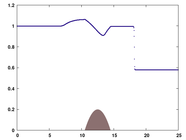
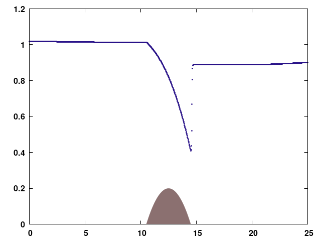
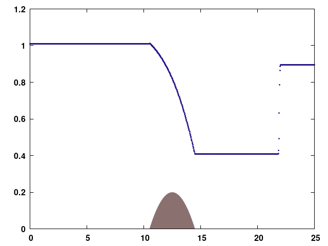
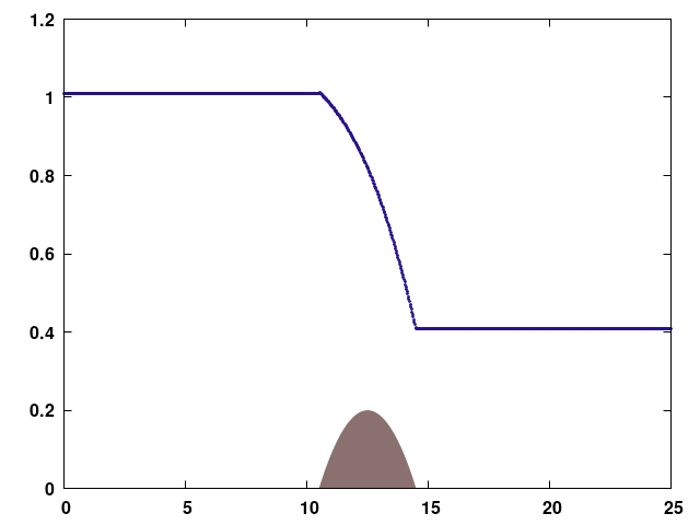
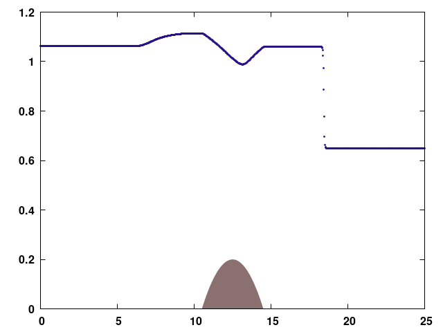
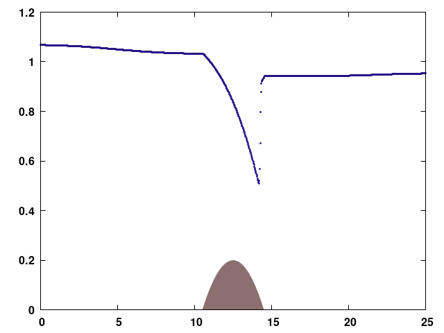
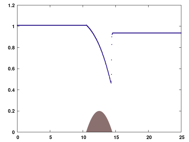
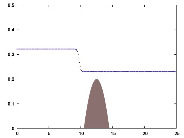
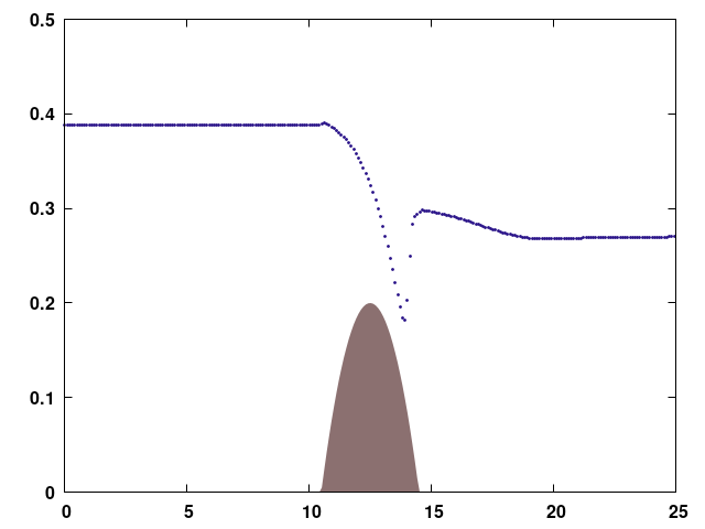
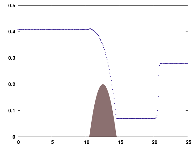
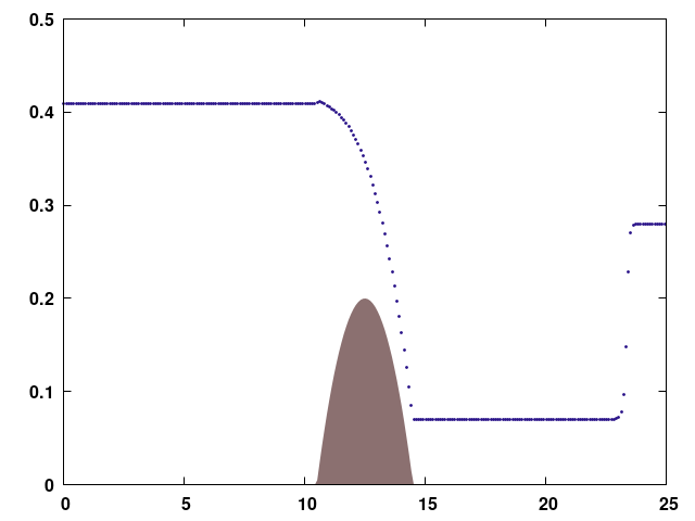
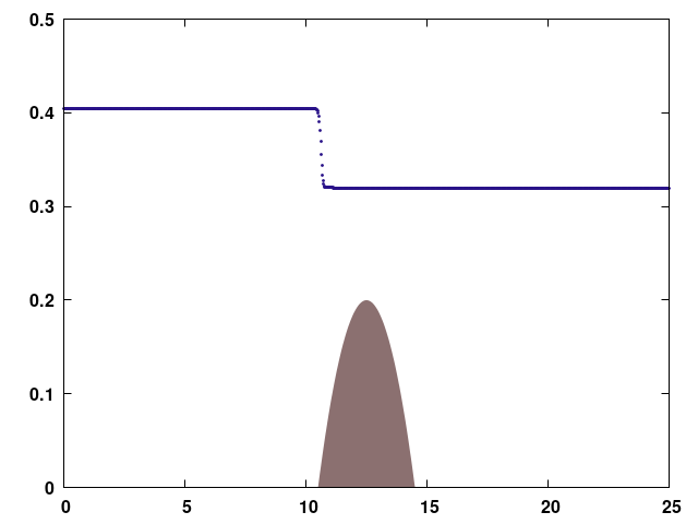
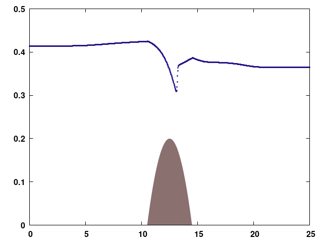
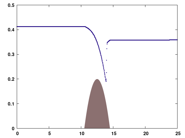
The goal is to find out whether or not the discrete dynamical system (35) with (17) and (40) reaches a steady state. If a steady state is reached, then we are interested to see the way this state is determined by the initial water level $\eta$. As in the aforementioned papers, we consider the cases corresponding to values of the left boundary flux $q_{0}=1.53$m²/s and $q_{0}=0.18$m²/s.

Figures 1 and 2 illustrate the behavior of the numerical solution when it develops a moving or a steady shock.

	$t=5$s	$t=20$s	$t=150$s	$t=200$s
Water level [m]					$\eta=0.58$m
Water level [m]					$\eta=0.65$m
	$x$ [m]	$x$ [m]	$x$ [m]	$x$ [m]

Figure 1: Snapshots from the steady solution of a flow over a bump. Moving (first row) and steady (second row) shocks for $q_{0}=1.53$m²/s.

	$t=5$s	$t=20$s	$t=150$s	$t=200$s
Water level [m]					$\eta=0.23$m
Water level [m]					$\eta=0.32$m
	$x$ [m]	$x$ [m]	$x$ [m]	$x$ [m]

Figure 2: Snapshots from the steady solution of a flow over a bump. Moving (first row) and steady (second row) shocks for $q_{0}=0.18$m²/s.

Propagation of a wave
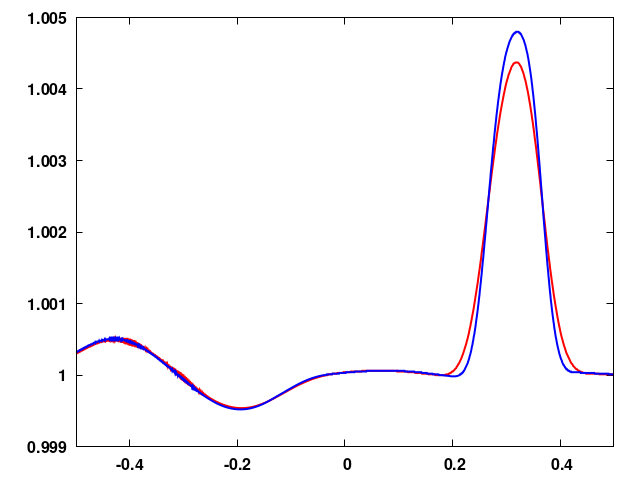
The second test problem concerns the propagation of a wave over a bump. This kind of the test was firstly considered by LeVeque [37]. The soil topography is defined by

$$z(x)=\left\{\begin{array}[]{ll}0.25(\cos{(\pi x/0.1)}+1),&{\rm if}\;|x|<0.1\\ 0,&{\rm otherwise}\end{array}\right.$$ (50)

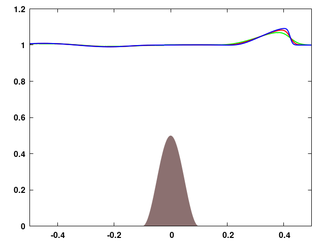
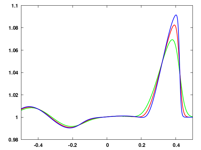
over the domain of flow $\Omega=[-1.25,1.25]$. The initial datum is a flat surface perturbed by a small crest

$$(z+h)|_{t=0}=\left\{\begin{array}[]{ll}1+\epsilon&{\rm if}\;-0.4<x<-0.3\\ 1,&{\rm otherwise}\end{array}\right..$$ (51)

There are no boundary conditions. The water level on $\Omega$ at a given moment of time calculated with our numerical scheme is pictured in Figure 3 for $x\in[-0.5,0.5]$.

	$\epsilon=0.2$	$\epsilon=0.2$	$\epsilon=0.01$
Water level [m]
	$x$ [m]	$x$ [m]	$x$ [m]

Figure 3: Snapshot at $t=0.7$s from the propagation of a wave over a bump. This test problem was accomplished for the gravitational acceleration $g=1$. Left picture presents the soil topography and the water level given by the numerical solution with $N$ interior points: $1000$ - green, $2000$ - red, $4000$ - blue. The picture in the middle represents a zoom of the left image. A similar zoom for the numerical solution (with $2000$ and $4000$ interior points) for a smaller height of the crest is drawn in the right picture.

4.1.2 Thacker Problem

The oscillation of the water level in a convex soil surface or the oscillatory motion of the sea water in the shoreline are very natural phenomena. A very difficult problem here is that a singularity appears at the wet/dry contact between water and soil surfaces. Different numerical schemes were proposed to solve this kind of problem and among them we mention [6].

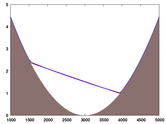
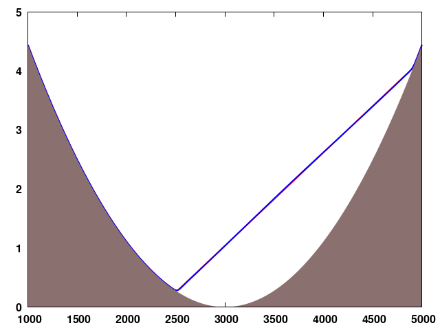
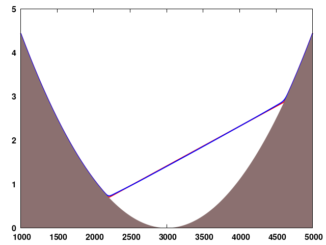
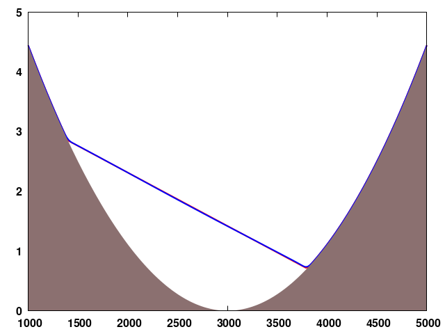
Thacker problem is a useful test to check the ability of a numerical scheme to catch and highlight the propagation of a wet/dry front. Moreover, this problem can be exactly solved [49, 44]. Thus, once can take advantage of its analytic solution to verify the accuracy of the numerical scheme. Thacker solution for 1-D shallow water equations was obtained in the absence of vegetation ($\theta=1$), for $\mathfrak{t}^{p}=\boldsymbol{0}$ and $\mathfrak{t}^{s}=h\tau\boldsymbol{v}$ in (1), where $\tau$ is a proportionality coefficient, for a soil surface $z(x)$ of parabolic shape, and for a water velocity which does not depend on space variable, i.e. $\boldsymbol{v}(t,x)=\boldsymbol{f}(t)$.

For the case of a 1D flow, the general solution is given by

$$\begin{split}h(t,x)+z(x)=&\left(\displaystyle\frac{x}{g}-\displaystyle\frac{\psi(t)}{2g\lambda_{1}\lambda_{2}}+\displaystyle\frac{\alpha}{\lambda_{1}\lambda_{2}}\right)\psi(t)+\eta_{0},\\ u(t)=&A\exp{\lambda_{1}t}+B\exp{\lambda_{2}t},\end{split}$$ (52)

where

$$\psi(t)=A\lambda_{2}\exp{\lambda_{1}t}+B\lambda_{1}\exp{\lambda_{2}t},$$

$\lambda_{1}$ and $\lambda_{2}$ solve

$$\left\{\begin{split}\lambda_{1}+\lambda_{2}=&-\tau\\ \lambda_{1}\lambda_{2}=&g\partial^{2}_{x}z(x)\end{split}\right.$$

and

$$\alpha=\partial_{x}z(x)-x\partial^{2}_{x}z(x).$$

In (52), $A$ and $B$ are integration constants. Depending on $z(x)$ and $\tau$, the solutions $\lambda_{1}$ and $\lambda_{2}$ can be real or complex numbers. An oscillating solution is obtained if

$$\tau^{2}-4g\partial^{2}_{x}z(x)<0.$$

In our numerical experiment, we chose

$$\begin{array}[]{l}z(x)=z_{m}\left(\displaystyle\frac{2x}{L}-1\right)^{2},\quad x\in[0,L],\\ A+B=0;\quad A-B={\rm i}u_{0},\end{array}$$

where the constants $z_{m}$, $L$ and $u_{0}$ are free parameters.

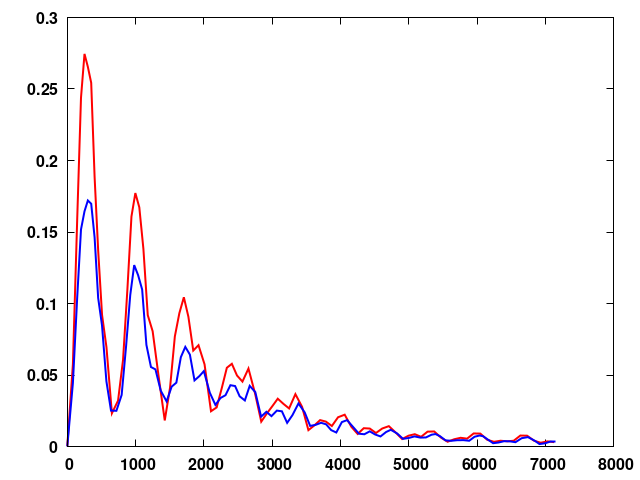
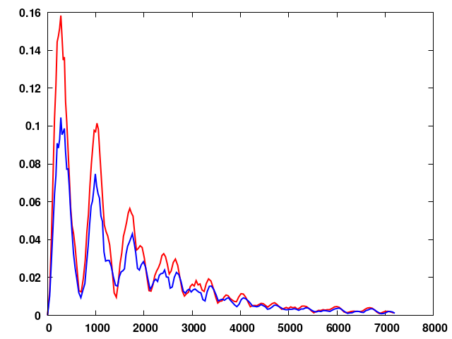
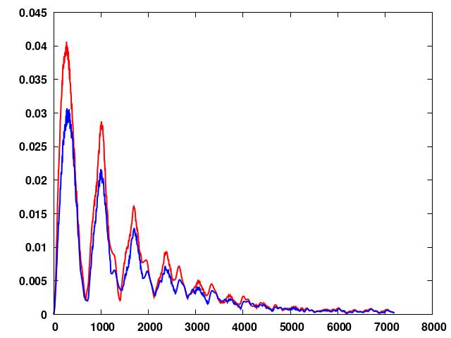
We compare the results from our numerical scheme (using different formulas (17) or (19) for the interface values of $(\theta h)^{s}$) with the analytic Thacker solution: the evolution of the errors between exact and numerical solutions in Figure 4 and the dynamics of the water surface in Figure 5. In all simulations, we use $z_{m}=10{\rm m}$, $L=6000{\rm m}$, $u_{0}=5{\rm m}\cdot{\rm s}^{-1}$ and $\tau=0.001{\rm s}^{-1}$. The artificial viscosity is defined by (40).

	$\delta x=10$m	$\delta x=5$m	$\delta x=1$m
Error
	time [s]	time [s]	time [s]

Figure 4: Thacker Problem: time evolution of the error $err=||(hu)^{app}-(hu)^{ex}||_{\infty}$ of discharge between the analytic and numerical solutions, when the numerical one was calculated with the arithmetic mean formula (19), blue line, and the upwind formula (17), red line, for $(\theta h)^{s}$, respectively. This evolution of the error is represented for three space step-sizes $\delta x$ and one can observe that the error is decreasing with $\delta x$.

	$t=300$s, $err=0.0435$	$t=600$s, $err=0.0513$	$t=900$s, $err=0.0460$	$t=1200$s, $err=0.0348$
Water level [m]
	$x$ [m]	$x$ [m]	$x$ [m]	$x$ [m]

Figure 5: Thacker Problem: dynamics of the water level. Numerical (blue) and analytic (red) solutions. The error between these two solutions is given by $err=||((h+z)^{app}-(h+z)^{ex})/(h+z)^{ex}||_{\infty}$.

4.1.3 Riemann Problem

We remind that Riemann problem for shallow water equations with topography and vegetation requires to solve the equations for piecewise constant initial data

$$\left.(h,u)\right|_{t=0}=\left\{\begin{array}[]{ll}(h_{L},u_{L}),&x<0\\ (h_{R},u_{R}),&x>0\end{array}\right.$$

and piecewise constant soil surface and porosity functions

$$(\theta,z)(x)=\left\{\begin{array}[]{ll}(\theta_{L},z_{L}),&x<0\\ (\theta_{R},z_{R}),&x>0\end{array}\right..$$

The problem was extensively analyzed [33, 34, 4, 21, 17, 1] for the case of constant vegetation, but there are only few results when the porosity is a variable function [19, 9]. Perhaps, this scarcity of results is due to the fact that the problem is less tractable for the case of jumps in both soil and porosity functions.

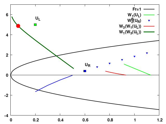
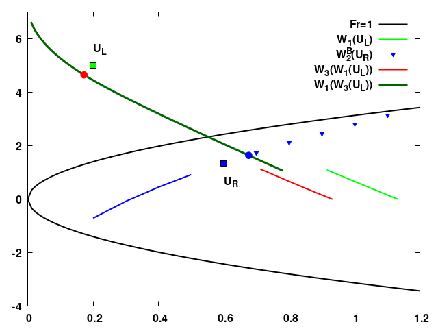
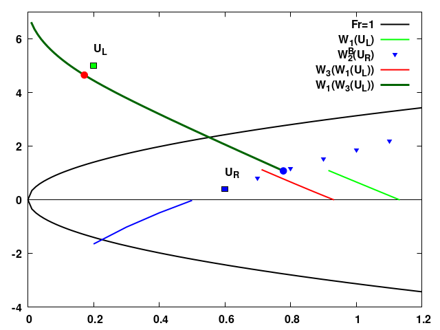
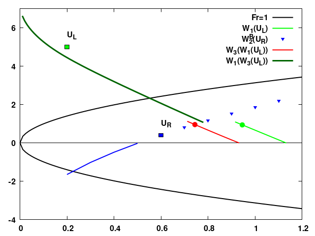
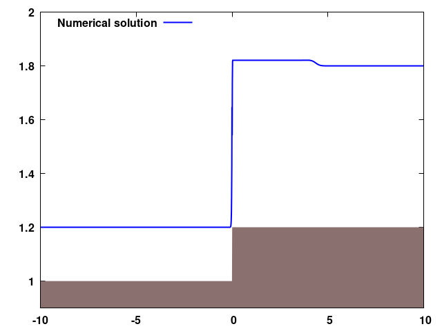
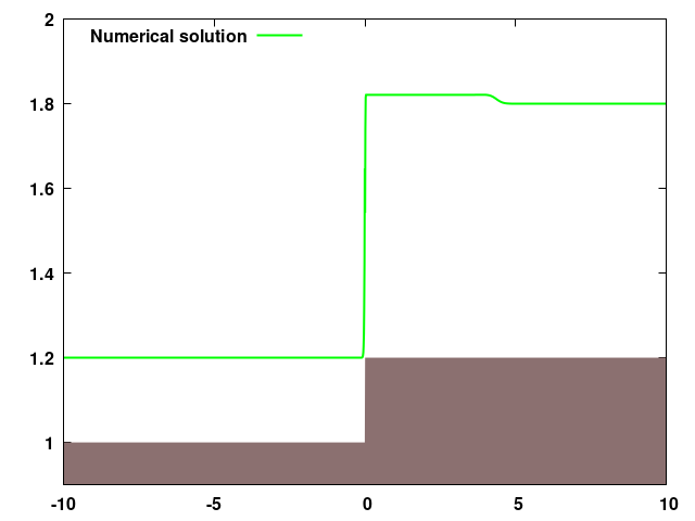
Usually, the solution of the problem is sought as a bunch of simple waves (shock waves, rarefaction waves and standing waves) ordered on the base of the entropy principle, [31]. We remark that such a solution may not exist or it can exist (being unique or non-unique). We perform a comparative study on these three cases. The data for each case are given in Table 1.

	Non-existence	Uniqueness	Two solutions
$(h,u)_{L}$	$(0.2,5.0)$
$(h,u)_{R}$	$(0.6,0.4)$	$(0.6,1.34)$	$(0.6,0.4)$
$(\theta,z)_{L}$	$(0.3,1.0)$	$(0.8,1.0)$
$(\theta,z)_{R}$	$(1.0,1.2)$

Table 1: Data for Riemann problem

The choice of these data was suggested by some cases analyzed in [34].

	Non-existence	Uniqueness	Two solutions
	$z_{R}-z_{L}=0.2,\,\frac{\theta_{L}}{\theta_{R}}=0.3$	$z_{R}-z_{L}=0.2,\,\frac{\theta_{L}}{\theta_{R}}=0.8$	$z_{R}-z_{L}=0.2,\,\frac{\theta_{L}}{\theta_{R}}=0.8$
u [m/s]
	h [m]	h [m]	h [m]	h [m]
Water level [m]			Solution not revealed
Water level [m]				Solution not revealed
	x [m]	x [m]	x [m]	x [m]

Figure 6: Riemann problem for three different initial data. The first row of pictures contains the simple wave curves in the phase space $(h,u)$. The last two rows of pictures include the graphics of the numerical and exact solutions (if they exist) of the free water surface at $t=1.5$s. The numerical solutions represented in the second and third rows are calculated using formulas (19) and (17), respectively.

The analytic solutions for the Riemann problem are calculated using the path connection introduced in [25] and the algorithms described in [29].

Figure 6 summarizes the results for the Riemann problem in the three cases (non-existence, uniqueness and two solutions) associated to the initial data given in Table 1.

4.2 External Validation

Numerical data incorporate two main errors: one given by the approximation of the physical phenomena by a mathematical model and the other one given by the approximation of the solution of the mathematical model. Consequently, a good fit of the numerical data with experimental data validates both the mathematical model and the numerical scheme. Thus, for real world applications, it is essential to confront the numerical data with the experimental data.

We test the mathematical model and the numerical solution considering the following problems:

1. dam break flow over a triangular bump,

2. downslope flow through rigid vegetation,

3. flow on a convex-concave vegetated soil surface,

4. simulation on Paul’s Valley (2D).

The first two tests simulate solutions for experiments with measured data, while the last two tests target the qualitative behavior of the solution.

4.2.1 Dam Break Flow Over a Triangular Bump

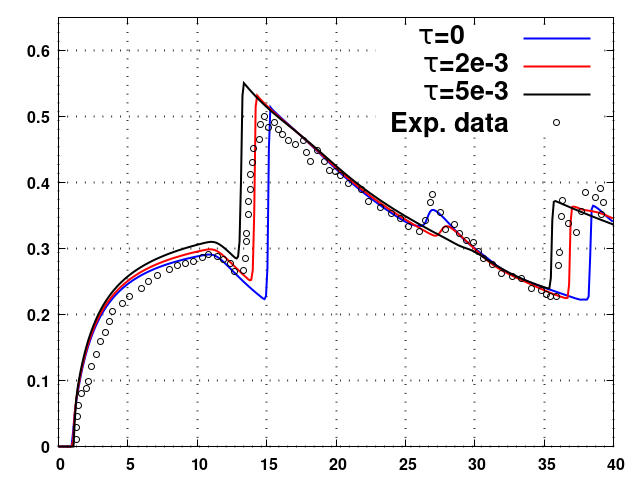
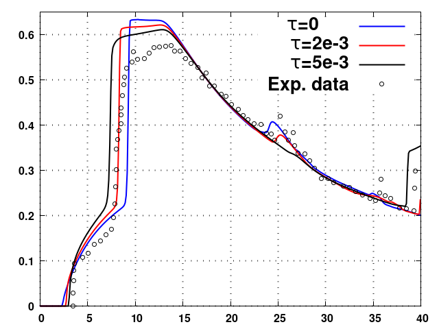
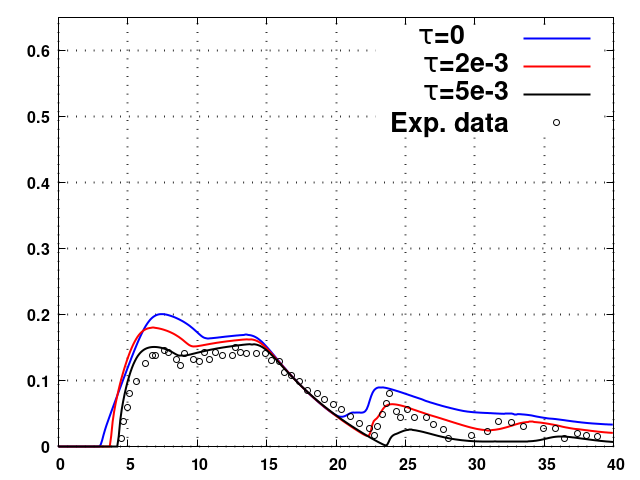
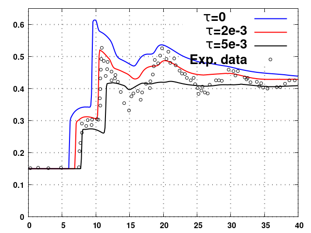
First, we consider the CADAM test case of the dam break flow propagation in an impermeable channel with a symmetric triangular bump [40, 14, 23]. The layout of this experiment and the initial state of the water at rest are presented in Figure 7.

Figure 7: Scheme of the experimental installation for the triangular bump test

Several gauges $G_{i}$ are placed in the channel to measure the water depth evolution once the gate retaining the water volume from the left side is suddenly removed.

In this experiment, the cover plant is absent: $\theta=1$. For the frictional term $\mathfrak{t}^{s}_{a}=\alpha_{s}(h)|\boldsymbol{v}|v_{a}$, we consider the Darcy-Weisbach formula

$$\alpha_{s}(h)=\tau,$$ (53)

where $\tau$ is constant. For this setup, we performed several numerical simulations with different values for $\tau$. The experimental data are extracted from the graphics reported in [23], Figure 5. The results are synthesized in Figure 8.

	G4	G10	G13	G20
Water depth [m]
	Time [s]	Time [s]	Time [s]	Time [s]

Figure 8: Flow over a triangular bump

Note that our solution is in agreement to the measured one (for all four gauges) for $\tau\approx 2e-3$.

We repeated the numerical simulations using Stickler-Manning formula

$$\alpha_{s}(h)=\frac{n^{2}}{h^{1/3}}$$ (54)

with $n^{2}\approx 0.003$m^1/3 and we have seen that there is no significant difference from the previous case.

4.2.2 Flow Over a Slope with Vegetation

The flow in the presence of vegetation is more complex than the one on bare soil and perhaps this explains a scarcity of the reported data.

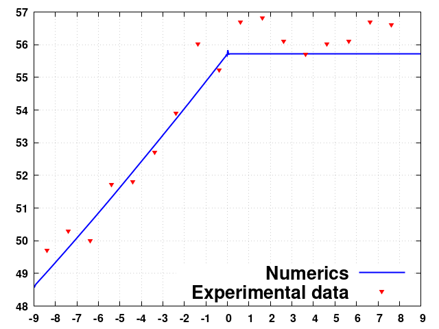
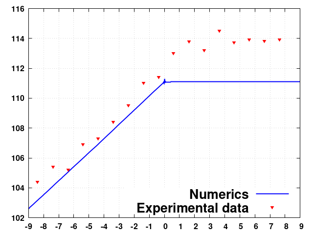
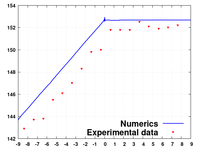
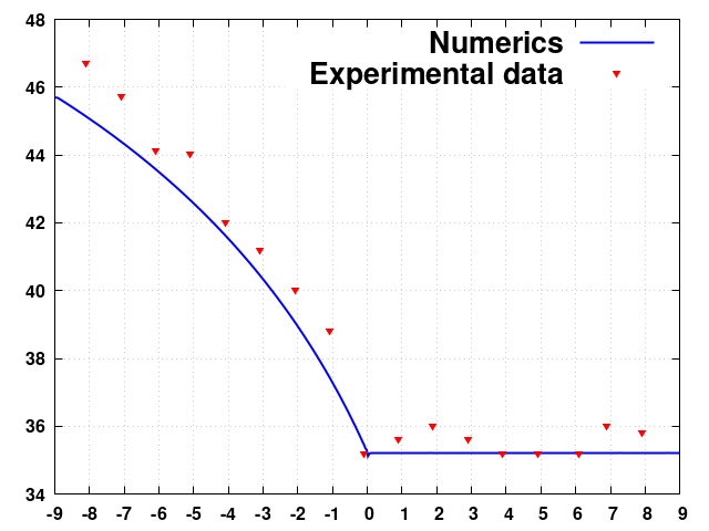
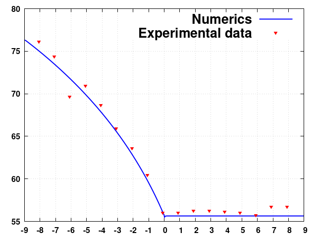
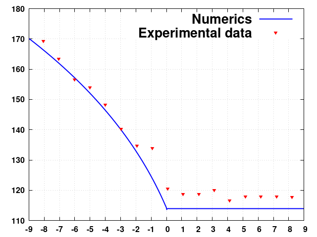
Here, we compare our results with the ones reported in [13]. Briefly, the experimental installation consists of an $18$m long and $1$m width laboratory flume with a longitudinal bottom slope $S=1.05{\rm mm}/{\rm m}$. The vegetation is modelled using uniformly distributed emergent circular cylinders of radius $R_{c}=5$mm. The density of vegetation is $N=81$ cylinder/m². This type of vegetation allows the estimation of the porosity by

$$\theta=1-N\pi R_{c}^{2}=0.99336.$$

To obtain the parameters $\alpha_{p}$ and $\alpha_{s}(h)$, we use the steady state values of $h$ and $u$ reported [13] for different values of the water discharge $q=hu$. These values can be theoretically estimated from relations

$$\begin{array}[]{l}\theta hu=q,\\ g\theta hS=(\alpha_{p}h(1-\theta)+\theta\alpha_{s}(h))u^{2}.\end{array}$$

One can estimate $\alpha_{s}(h)$ from the data for bare soil and then use it to calculate $\alpha_{p}$ using the data for uniformly distributed vegetation. Thus, if Darcy-Weisbach formula is used, one finds that $\tau$ runs in $[6.508084,9.00375]\cdot 10^{-3}$ and $\alpha_{p}$ takes values in $[73.20,80.20]$. For the case of Strickler-Manning formula, one finds $n^{2}\in[2.893622,3.178546]\cdot 10^{-3}$ and $\alpha_{p}\in[72.27832,77.97572]$.

These estimations indicate that Strickler-Manning formula is more appropriate than Darcy-Weisbach formula to be used for this kind of flow.

For testing numerical data, we choose the experiment of water flow on a partial vegetated bottom surface. We use Strickler-Manning formula with the parameters

$$n^{2}=3.005785\cdot 10^{-3}{\rm m}^{1/3},\quad\alpha_{p}=74.7643{\rm m}^{-1}.$$

These values correspond to the Strickler $K=57.099$ and drag coefficient $C_{D}=1.1738$.

Figure 9 includes the numerical and experimental data for six different steady configurations. The experimental data are extracted from the graphics reported in [13], Figure 8.

	$Q=7$ l/s	$Q=15$ l/s	$Q=21$ l/s
Water level [mm]
	x [m]	x [m]	x [m]
	$Q=7$ l/s	$Q=15$ l/s	$Q=50$ l/s
Water level [mm]
	x [m]	x [m]	x [m]

Figure 9: Flow over a slope with vegetation

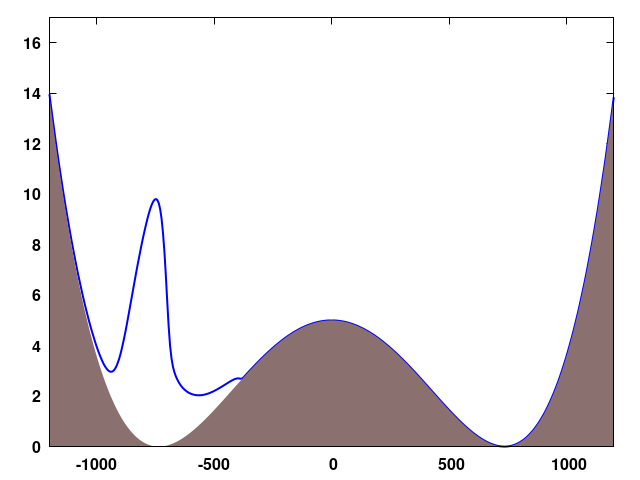
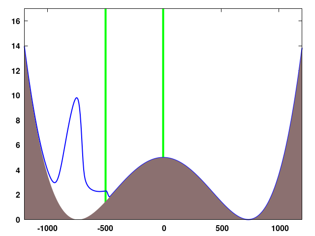
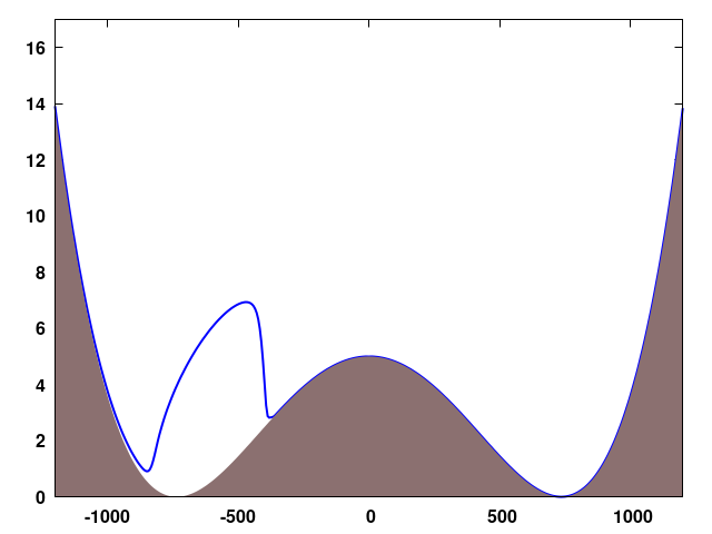
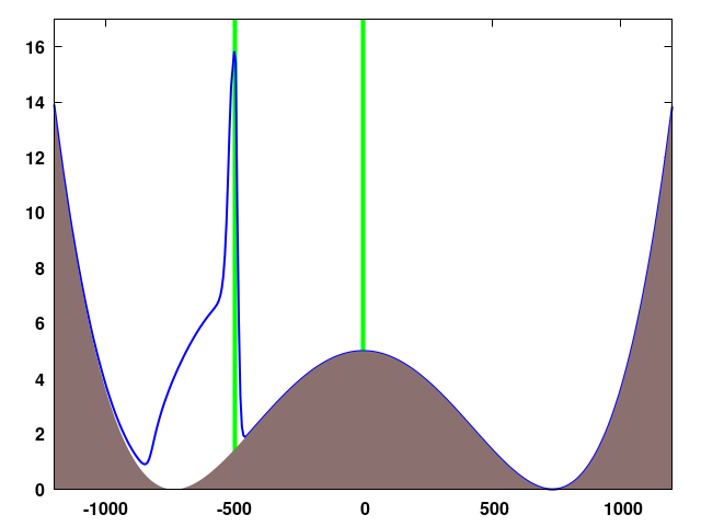
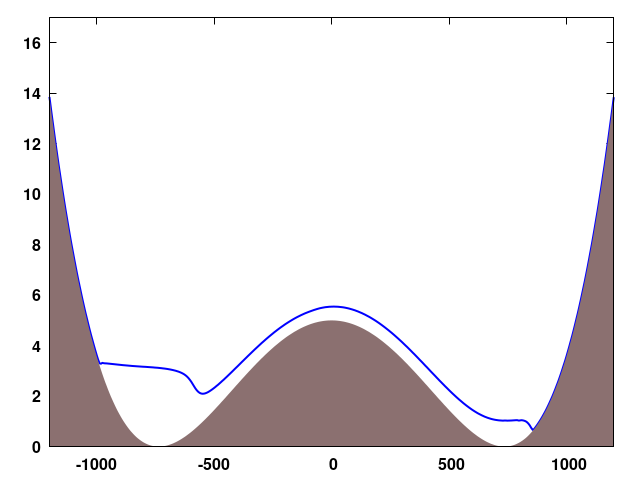
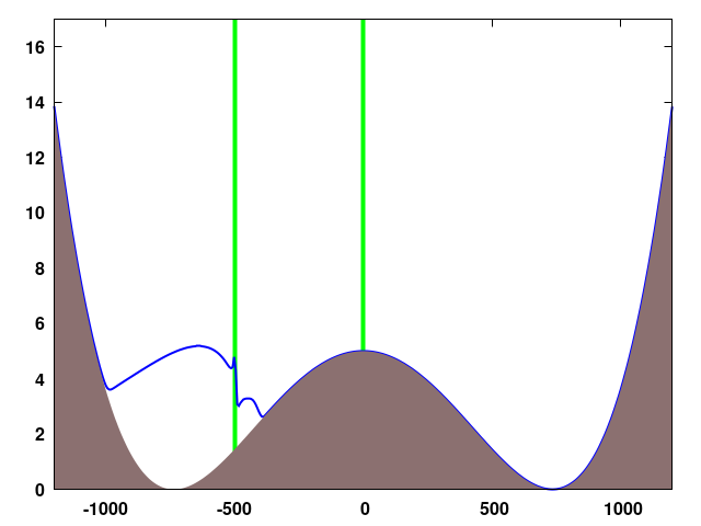
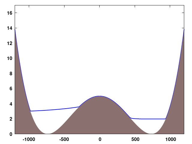
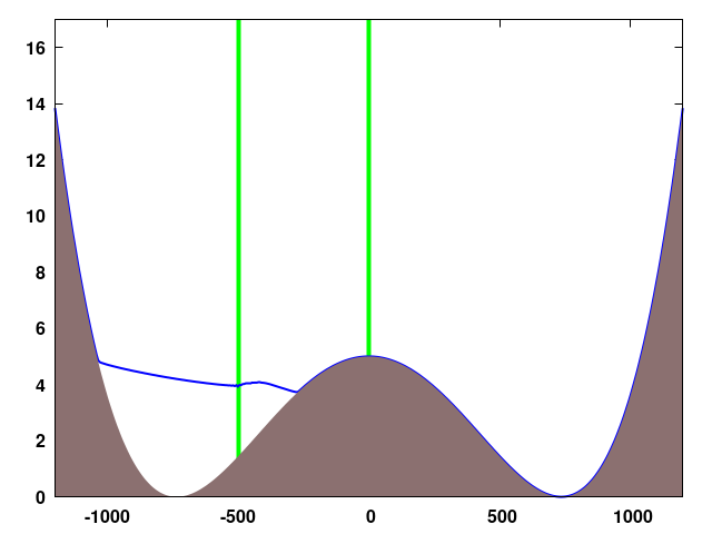
4.2.3 Flow Over a Convex-Concave Vegetated Soil Surface

There are two reasons for considering the flow over a convex-concave vegetated soil surface: to highlight the influence of the cover plant on the water flow dynamics and to emphasize the ability of our numerical scheme not only to preserve the lake as an equilibrium point, but to asymptotically reach it.

We consider a topography with the surface given by a fourth degree polynomial on $[-L,L]$

$$z(x)=h_{m}\left[\sqrt{\frac{h_{b}}{h_{m}}}-\frac{1}{L^{2}}\left(1+\sqrt{\frac{h_{b}}{h_{m}}}\right)x^{2}\right]^{2},$$

where $L=1500$m, $h_{m}=50$m and $h_{b}=5$m. For this configuration, the mathematical equilibrium point may consist of one or two lakes. Our model is run for two different configurations, without vegetation and with vegetation, respectively. We use Stickler-Manning formula (54) with $n^{2}=0.003{\rm m}^{1/3}$. The initial conditions

$$h_{0}=\left\{\begin{array}[]{ll}2,&{\rm if}\;x\leq-L/3\\ 0,&{\rm if}\;x>-L/3\end{array}\right.,\quad v_{0}=0$$

are identical for both configurations. For the configuration with vegetation, we add

$$\alpha_{p}=79.3,\quad\theta=\left\{\begin{array}[]{ll}0.9,&{\rm if}\;-L/3\leq x\leq 0\\ 1,&{\rm otherwise}\end{array}\right..$$

	Bare soil	Vegetated soil
Water level [m]
Water level [m]
Water level [m]
Water level [m]
	$x$ [m]	$x$ [m]

Figure 10: Dumping effect of water flow. The left column of images shows the states of the solution at four different moments of time ($t=40,\;60,\;200,\;400$ s) for the configuration without vegetation. The solution for the configuration with vegetation is represented in the right column at the same moments of time. Remark the tendency of the water to form two lakes in the first configuration and only one lake in the second configuration.

Figure 10 illustrates the numerical solution of the water surface for these two configurations.

4.2.4 Simulation on Paul’s Valley

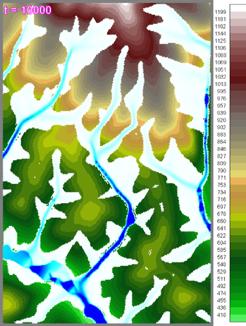
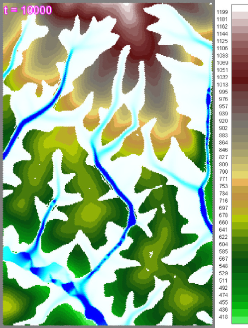
Unfortunately, we do not have data for the water distribution, plant cover density and measured velocity field in a hydrographic basin to compare our numerical results with. However, to be closer to reality, we have used GIS data for the soil surface of Paul’s Valley and accomplished a theoretical experiment: starting with a uniform water depth on the entire basin and using different cover plant densities, we run the 2D version of our scheme (a flow modulus of ASTERIX) on a hexagonal network. To generate an arbitrary hexagonal network from an arbitrary raster GIS data, we use the method introduced in [26]. Figure 11 shows that the numerical results are consistent with direct observations concerning the water time residence in the hydrographic basin.

Figure 11: Snapshot of water distribution in Paul’s Valley hydrographic basin. Direct observations indicate that the water time residence depends on the density of the cover plant. Our numerical data are consistent with terrain observations: the water drainage time is greater for the case of higher cover plant density. $\theta=0.97$ and $\theta=0.65$ for the left and right picture, respectively.

5 Discussion, Conclusions and Further Research

The effect of vegetation on the water circulation in a continuum soil-plant-atmosphere can relatively be easy described, but it is hardly quantifiable. The canopy of vegetation intercept and store a certain amount of rain, the stem of plant generate a resistance force to the water running on the soil surface and the plant roots modify the water infiltration rate into soil. To quantify these physical processes and put them in a mathematical model is a big challenge and it requires new mathematical concept, experimental results and numerical simulations.

The mathematical model (1) is simplified as possible as can be to retain essential interaction factors and to be mathematical tractable. The mathematical model (1) belongs to the class of hyperbolic systems and it has certain distinctive feature that raises special difficulties when one elaborates a numerical scheme to approximate its solution. Namely,

(a) the system becomes singular for $h=0$;

(b) the hyperbolic system has a non-conservative form and its coefficients depend on the space variable, non-homogeneous hyperbolic system;

(c) there can be a dependence of the system of the derivatives of discontinuous functions, soil surface and/or porosity functions;

(d) the unknown water depth function $h(t,x)$ must be a positive function.

We appreciate that the finite volume method for the space discretization of the system is the most fitted method. It allows one to treat the non-conservative product, see (11), and then perform the approximations (14-3), (17), (18) and (19). By introducing the flux terms (15-1), (15-2), (16), we were able to ensure the positivity of $h$.

To solve the problem of the singularities introduced by $h=0$, we perform a first order fractional time step method. In the presence of frictional force or drag resistance force, the second equation in the scheme (34) is nonsingular even if $h=0$.

When validating using Riemann problem, Section 4.1.3, we should observe that for defining the standing waves, one needs to augment the shallow water equations with an additional principle: either path connection or an energetic principle.

For us, testing the numerical scheme against the solution of Riemann problem, given by a composition of simple waves, is instructive in two ways. In one way, it is interesting to find out how the numerical scheme works in all the possible situations: non-existence, uniqueness and non-uniqueness of the solutions. On the other way, the numerical scheme does not “see” the second principle invoked in the construction of the standing waves since it is based on the approximation principles of the operators and functions appearing in the shallow water equations. Thus, when one compares the numerical solution to the analytic solution, the question of compatibility between the two kind of principles can be raised. However, the case of the Godunov type approximation schemes is different since these schemes are obtained on the basis of the (exact or approximate) solution of the Riemann problem. We observed that it does not matter whether the quantity $(\theta h)^{s}_{(i,j)}$ is calculated using (18) or (19) in the cases of non-existence or uniqueness of the solution. But in the case of multiple solutions, different approximation formulas of the gradient of the free surface lead to different solutions. Also, we draw attention that by non-existence case we mean ”the non-existence of a composite wave as a solution of the Riemann Problem”, which is different from ”the non-existence of a solution of the Riemann Problem”. Consequently, the numerical solution can be an approximation of the true solution or can be a fictitious mathematical object.

Note that the transition from the non-existence to the existence but not uniqueness of the solution for Riemann problem is controlled only by the size of the jump in $\theta$.

The numerical simulations for the steady solution case of a flow over a bump (Section 4.1.1) suggest the following conjecture.

Conjecture.

There is a value $q^{M}$ such that for any $q\in(0,q^{M})$ there are two threshold values $0.2\leq\eta_{1}(q)<\eta_{2}(q)$ such that:

1. the numerical solution asymptotically reaches a state $(h^{\star},u^{\star})$;

2. the state $(h^{\star},u^{\star})$ casts into one of the following three distinct categories:

   1. for any $\eta\in(0.2,\eta_{1})$, it develops a moving shock which goes out of the domain $\Omega$ after a while,

   2. for any $\eta\in(\eta_{1},\eta_{2})$, it has a steady shock located in the domain occupied by the bump,

   3. for any $\eta>\eta_{2}$, it is smooth (no shock).

Case (a) of the conjecture is illustrated on the first row of pictures in Figures 1 and 2; case (b) is also illustrated on the second row of pictures in the same figures.

A common problem in many countries, Romania being a typical example, is land deforestation with severe flood effects. The test proposed in Section 4.2.3 was considered to emphasize the protective role of vegetative barrier against such natural disasters. Remark that in the configuration with vegetation, the water does not anymore cross the knoll since it loses part of its energy due to the friction with plants, see Figure 10. Note that our numerical method is not only well-balanced, but it is capable to produce solutions that reach different equilibrium states (depending on the initial data and the values of the parameters). It should be also remarked that the porosity $\theta$ plays the role a control function to get different equilibrium points: one or two lakes.

Water flow in hydrographic basins is more complicated due to variations in soil topography and in vegetation diversity. In contrast to the 1D cases where we were able to easily simulate the soil data, we now need 2D land and vegetation data to be closer to reality. Data for soil surface can be obtained from topographic maps, GIS, LiDAR etc. For the purpose of modeling, one needs an interface to transfer data between different scales. In this sense, we used the tool built and described in [26]. Simulation on Paul’s Valley (with no rain and infiltration) was considered in Section 4.2.4 as a first step to get closer to the interesting cases from ecology, biology, hydrology and terrestrial sciences. An important variable for such a hydrographic basin is the amount of water leaving the basin. This variable can be measured using the relative amount $q$ of water in the basin at the moment of time $t$ given by

$$q(t)=\displaystyle\frac{\displaystyle\int_{\Omega}h(t,x){\rm d}x}{\displaystyle\int_{\Omega}h(0,x){\rm d}x}.$$

Figure 12: Time evolution of the water content in Paul’s Valley hydrographic basin with ASTERIX (left picture) and CAESAR (right picture).

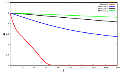
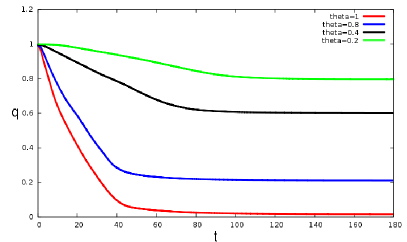
Figure 12 shows the results for the water content in Paul’s Valley basin obtained with our models ASTERIX and with CAESAR-Lisflood-OSE [24].

A general issue relates to whether higher cover plant densities can prevent soil erosion and flood or not. Both pictures show that if the cover plant density is increasing then the decreasing rate $\dot{q}$ of $q$ is smaller. We can think at a “characteristic velocity” of the water movement in the basin and this velocity is in a direct relation with $\dot{q}$. We can now speculate that smaller values of $\dot{q}$ imply softer erosion processes.

This valley belongs to Ampoi’s catchment basin. Flood generally appears when the discharge capacity of a river is overdue by the water coming from the river catchment area. Our pictures show that higher cover plant densities imply smaller values of $\dot{q}$ which in turn give Ampoi River the time to evacuate the water amount flowing from the valley.

As conclusions, we have presented a mathematical model able to take into account the effects introduced by plants on the water flow on soil surface and we have introduced a numerical scheme to approximate its solution. The numerical scheme is of first order in time and space accurate and is able to model a large class of physical phenomena, waves propagation, backward wave reflection induced by obstacles or filter band vegetation, oscillating flow, one or multiple lake formation. The scheme is relatively simple to be implemented in a more complex model like soil erosion.

As current research, we work on elaborating a methodology based on inverse method to estimate the hydrodynamics parameters $\alpha_{p}$ and $\alpha_{s}$ from in situ experimental measurements.

In the future, we intend to build up a coupled model – shallow water - soil erosion – to investigate the role of plants to mitigate the transport of the polluted soil particles from contaminated area to around area.

References

- [1] Nikolai Andrianov. Performance of numerical methods on the non-unique solution to the Riemann problem for the shallow water equations. Int. J. Numer. Meth. Fluids, 47:825–831, 2005.
- [2] Aronne Armanini and Valentina Cavedon. Bed-load through emergent vegetation. Advances in Water Resources, 129:250–259, 2019.
- [3] M J Baptist, V Babovic, J Rodriguez Uthurburu, M Keijzer, R E Uittenbogaard, A Mynett, and A Verwey. On inducing equations for vegetation resistance. Journal of Hydraulic Research, 45(4):435–450, 2007.
- [4] R Bernetti, V A Titarev, and E F Toro. Exact solution of the Riemann problem for the shallow water equations with discontinuous bottom geometry. Journal of Computational Physics, 227(6):3212–3243, March 2008.
- [5] F Bouchut. Nonlinear Stability of Finite Volume Methods for Hyperbolic Conservation Laws. Birkhäuser, Basel, 2004.
- [6] Scott F. Bradford and Brett Sanders. Finite-volume model for shallow-water flooding of arbitrary topography. Journal of Hydraulic Engineering, 128(3):289–298, 2002.
- [7] A Chinnayya, A Y LeRoux, and N Seguin. A well-balanced numerical scheme for the approximation of the shallow-water equations with topography: the resonance phenomenon. International Journal on Finite Volumes, 1:1–33, 2004.
- [8] TJ Coulthard, JC Neal, PD Bates, J Ramirez, GAM De Almeida, and GR Hancock. Integrating the LISFLOOD-FP 2D hydrodynamic model with the CAESAR model: implications for modelling landscape evolution. Earth Surface Processes and Landforms, 38:1897–1906, 2013.
- [9] Luca Cozzolino, Veronica Pepe, Luigi Cimorelli, Andrea D’Aniello, Renata Della Morte, and Domenico Pianese. The solution of the dam-break problem in the porous shallow water equations. Advances in Water Resources, 114:83 – 101, 2018.
- [10] Gianni Dal Maso, Philippe G. LeFloch, and François Murat. Definition and weak stability of nonconservative products. Journal de Mathématiques Pures et Appliquées. Neuvième Série, 74, 01 1995.
- [11] Olivier Delestre, Carine Lucas, Pierre-Antoine Ksinant, Frédéric Darboux, Christian Laguerre, and et al. SWASHES: a compilation of shallow water analyticsolutions for hydraulic and environmental studies. International Journal for Numerical Methods in Fluids, 72(3):269–300, 2013.
- [12] J C I Dooge. A general theory of the unit hydrograph. Journal of Geophysical Research, 64(2):241–256, 1959.
- [13] Victor Dupuis, Sébastien Proust, Céline Berni, and André Paquier. Combined effects of bed friction and emergent cylinder drag in open channel flow. Environmental Fluid Mechanics, 16(6):1173–1193, Dec 2016.
- [14] S. Erpicum, B.J. Dewals, P. Archambeau, and M. Pirotton. Dam break flow computation based on an efficient flux vector splitting. Journal of Computational and Applied Mathematics, 234(7):2143 – 2151, 2010.
- [15] Mohammed Seaid Fayssal Benkhaldoun. A simple finite volume method for shallow water equation. Journal of Computational and Applied Mathematics, 234:58–72, 2010.
- [16] U S Fjordholm, S Mishra, and E Tadmor. Well-balanced and energy stable schemes for the shallow water equations with discontinuous topography. Journal of Computational Physics, 230(14):5587–5609, 2011.
- [17] Fayssal Benkhaldoun Francisco Alcrudo. Exact solution of the Riemann problem for the shallow water equations with a bottom step. Computers & Fluids, 30:643 – 671, 2001.
- [18] Vincent Guinot. Multiple porosity shallow water models for macroscopic modelling of urban floods. Advances in Water Resources, 37:40 – 72, 2012.
- [19] Vincent Guinot. A critical assessment of flux and source term closures in shallow water models with porosity for urban flood simulations. Advances in Water Resources, 109:133 – 157, 2017.
- [20] O Hájek. Discontinuous differential equations. Journal of Differential Equations, 32(2):149–170, 1979.
- [21] Ee Han and Gerald Warnecke. Exact Riemann solutions to shallow water equations. Quart. Appl. Math., 72:407–453, 2014.
- [22] B.C. Peter Heng, Graham C Sander, and Cecil F Scott. Modeling overland flow and soil erosion on nonuniform hillslopes: A finite volume scheme. Water Resources Research, 45:W05423, 2009.
- [23] Tai-Wen Hsu, Shin-Jye Liang, and Nan-Jing Wu. Application of meshless swe model to moving wet/dry front problems. Engineering with Computers, 35(1):291–303, Jan 2019.
- [24] S Ion, D Marinescu, and S G Cruceanu. CAESAR-LISFLOOD-OSE. www.ima.ro/software/caesar\_lisflood\_OSE.htm, 2014.
- [25] S Ion, D Marinescu, and S G Cruceanu. Riemann problem for shallow water equation with vegetation. An. St. Univ. Ovidius, 26(2):145–173, 2018.
- [26] S Ion, D Marinescu, S G Cruceanu, and V Iordache. A data porting tool for coupling models with different discretization needs. Environmental Modelling & Software, 62:240–252, 2014.
- [27] S Ion, D Marinescu, A-V Ion, S G Cruceanu, and V Iordache. Water flow on vegetated hill. 1D shallow water equation type model. An. St. Univ. Ovidius, 23(3):83–96, 2015.
- [28] Stelian Ion, Dorin Marinescu, and Stefan Gicu Cruceanu. Overland flow in the presence of vegetation, 2013.
- [29] Stelian Ion, Dorin Marinescu, and Stefan Gicu Cruceanu. Constructive approach of the solution of the Riemann problem for shallow water equations with topography and vegetation. arXiv e-prints, 2019.
- [30] A Kurganov and G Petrova. A second-order well-balanced positivity preserving central-upwind scheme for the Saint-Venant system. Communications in Mathematical Sciences, 5(1):133–160, 2007.
- [31] Peter D. Lax. Hyperbolic systems of conservation laws II. Comm. Pure Appl. Math., 10:537–566, 1957.
- [32] Minh H. Le, Virgile Dubos, Marina Oukacine, and Nicole Goutal. A Well-balanced Finite Volume Scheme for Shallow Water Equations with Porosity: Application to Modelling Flow through Rigid Vegetation. In E3S Web of Conferences, volume 40, pages 1–8, 2018.
- [33] Philippe G. LeFloch and Mai Duc Thanh. The Riemann problem for the shallow water equations with discontinuous topography. Commun. Math. Sci., 5(4):865–885, 12 2007.
- [34] Philippe G. LeFloch and Mai Duc Thanh. A Godunov-type method for the shallow water equations with discontinuous topography in the resonant regime. Journal of Computational Physics, 230(20):7631 – 7660, 2011.
- [35] R L LeVeque. Time-Split Methods for Partial Differential Equations. PhD thesis, Stanford University, Stanford, California, USA, 1982.
- [36] R L LeVeque. Finite Volume Methods for Hyperbolic Problems. Cambridge University Press, Cambridge, UK, 2002.
- [37] Randal J. LeVeque. Balancing source terms and flux gradients in high-resolution Godunov methods: The quasi-steady wave-propagation algorithm. Journal of Computational Physics, 146:346–365, 1998.
- [38] J J McDonnell, M Sivapalan, K Vachéand S Dunn, G Grant, R Haggerty, C Hinz, R Hooper, J Kirchner, M L Roderick, J Selker, and M Weiler. Moving beyond heterogeneity and process complexity: A new vision for watershed hydrology. Water Resources Research, 43(7):W07301, 1–6, 2007.
- [39] V Michel-Dansaca, C Berthon, S Clain, and F Foucher. A well-balanced scheme for the shallow-water equations with topography. Computers & Mathematics with Applications, 72(3):568–593, 2016.
- [40] M W Morris. CADAM: Concerted action on dam break modeling — Final report, 2000. Report SR 571 HR Wallingford.
- [41] H M Nepf. Drag, turbulence, and diffusion in flow through emergent vegetation. Water Resources Research, 35(2):479–489, 1999.
- [42] S Noelle, N Pankratz, G Puppo, and J R Natvig. Well-balanced finite volume schemes of arbitrary order of accuracy for shallow water flows. Journal of Computational Physics, 213(2):474–499, 2006.
- [43] K G Renard, G R Foster, G A Weesies, and J P Porter. Rusle: Revised universal soil loss equation. Journal of Soil and Water Conservation, 46(1):30–33, 1991.
- [44] Joe John Sampson, Alan Easton, and Manmohan Singh. Moving boundary shallow water flow in a region with quadratic bathymetry. ANZIAM Journal, 49:C666–C680, 2007.
- [45] G Strang. On the construction and comparison of difference schemes. SIAM Journal on Numerical Analysis, 5(3):506–517, 1968.
- [46] SWAP: Soil water atmosphere plant. www.swap.alterra.nl, 2019.
- [47] SWAT+: Soil and water assessment tool. swat.tamu.edu/docs, 2019.
- [48] Jun Tang, Derek Causon, Clive Mingham, and Ling Qian. Numerical study of vegetation damping effects on solitary wave run-up using the nonlinear shallow water equations. Coastal Engineering, 75:21 – 28, 2013.
- [49] W.C. Thacker. Some exact solutions to the nonlinear shallow-water equations. Journal of Fluid Mechanics, 107:499–508, 1981.
- [50] W H Wischmeier. A rainfall erosion index for a universal soil-loss equation. Soil Science Society of America Journal, 23(3):246–249, 1959.
- [51] D A Woolhiser, R E Smith, and D C Goodrich. KINEROS: A kinematic runoff and erosion model: documentation and user manual. Technical report, ARS-77, U.S. Government, Washinton, D.C., USA, 1990.
- [52] J. G. Zhou, D. M. Causon, C. G. Mingham, and D. M. Ingram. The surface gradient method for the treatment of source terms in the shallow-water equations. Journal of Computational Physics, 168:1–25, 2001.