Nao Mishimanao.mishima@toshiba.co.jp1 \addauthorTatsuo Kozakayatatsuo.kozakaya@toshiba.co.jp1 \addauthorAkihisa Moriyaakihisa.moriya@toshiba.co.jp1 \addauthorRyuzo Okadaryuzo.okada@toshiba.co.jp1 \addauthorShinsaku Hiurahiura@eng.u-hyogo.ac.jp2 \addinstitutionCorporate Research and Development Center, Toshiba Corp. \addinstitutionUniversity of Hyogo Depth Sensing with Deaberration Network
Physical Cue based Depth-Sensing by Color Coding with Deaberration Network
Abstract
Color-coded aperture (CCA) methods can physically measure the depth of a scene given by physical cues from a single-shot image of a monocular camera. However, they are vulnerable to actual lens aberrations in real scenes because they assume an ideal lens for simplifying algorithms. In this paper, we propose physical cue-based deep learning for CCA photography. To address actual lens aberrations, we developed a deep deaberration network (DDN) that is additionally equipped with a self-attention mechanism of position and color channels to efficiently learn the lens aberration. Furthermore, a new Bayes L1 loss function based on Bayesian deep learning enables to handle the uncertainty of depth estimation more accurately. Quantitative and qualitative comparisons demonstrate that our method is superior to conventional methods including real outdoor scenes. Furthermore, compared to a long-baseline stereo camera, the proposed method provides an error-free depth map at close range, as there is no blind spot between the left and right cameras.
1 Introduction
Compared with multi-shot depth measurement methods such as structure from motion (SfM) [Agarwal et al.(2009)Agarwal, Snavely, Simon, Seitz, and Szeliski] and depth from defocus (DfD) [Subbarao and Surya(1994), Tang et al.(2017)Tang, Cohen, Price, Schiller, and Kutulakos, Guo et al.(2017)Guo, Alexander, and Zickler], a single-shot method is suitable for moving objects. One of the most successful single-shot methods is deep monocular depth estimation. Despite the remarkable progress of deep monocular depth estimation in recent years [Eigen et al.(2014)Eigen, Puhrsch, and Fergus, Godard et al.(2017)Godard, Mac Aodha, and Brostow, Fu et al.(2018)Fu, Gong, Wang, Batmanghelich, and Tao], it cannot estimate a correct depth map without sufficient contextual information due to the lack of a physical depth cue, for instance, in a scene without the ground.
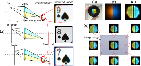
Instead of utilizing contextual information, color-coded aperture (CCA) methods can acquire a depth map based on a physical depth cue encoded in a single-shot image by inserting different types of color filters [Bando et al.(2008)Bando, Chen, and Nishita, Kim et al.(2012)Kim, Lee, Hayes, and Paik, Chakrabarti and Zickler(2012), Lee et al.(2013)Lee, Kim, Jung, Hayes, and Paik, Martinello et al.(2015)Martinello, Wajs, Quan, Lee, Lim, Woo, Lee, Kim, and Lee, Paramonov et al.(2016)Paramonov, Panchenko, Bucha, Drogolyub, and Zagoruyko, Moriuchi et al.(2017)Moriuchi, Sasaki, Mishima, and Mita] into the lens aperture as shown in Figure 2b. As shown in Figure 2a, color and blur radius vary according to the distance from the focus distance. Conventional CCA methods assume an ideal lens for simplifying analytical modeling of defocus blur. However, actual lenses have shift-variant point spread functions (PSFs) distorted according to the position of the image sensor by lens aberrations such as field curvature, coma or lateral chromatic aberration as shown in Figure 2e. Furthermore, the depth cues often disappear because of several uncertainties, such as saturation, soft shadow, dark color and large blur. These uncertainties are not treated distinctly in conventional methods [Bando et al.(2008)Bando, Chen, and Nishita, Kim et al.(2012)Kim, Lee, Hayes, and Paik, Chakrabarti and Zickler(2012), Lee et al.(2013)Lee, Kim, Jung, Hayes, and Paik, Martinello et al.(2015)Martinello, Wajs, Quan, Lee, Lim, Woo, Lee, Kim, and Lee, Paramonov et al.(2016)Paramonov, Panchenko, Bucha, Drogolyub, and Zagoruyko, Moriuchi et al.(2017)Moriuchi, Sasaki, Mishima, and Mita, Haim et al.(2018)Haim, Elmalem, Giryes, Bronstein, and Marom].
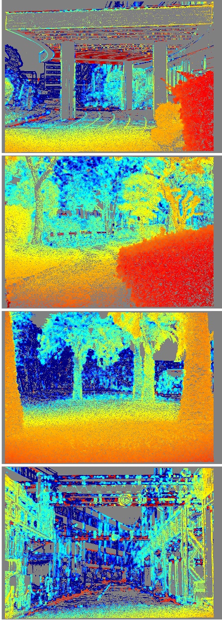
In this paper, we propose a physical cue-based deep learning to overcome the differences between the analytical model and the actual one. In order to estimate a correct depth map under shift-variant PSFs, we add positional information as an additional branch by a self-attention mechanism [Zhang et al.(2018)Zhang, Goodfellow, Metaxas, and Odena]. It also couples additional color channels to solve dependency on object colors for handling various complex color pattern correctly. To handle various uncertainties, we improve the loss function based on Bayesian deep learning [Kendall and Gal(2017)] for stabilizing the training. As shown in Figure 1, We demonstrate that our method is superior to a conventional method in quantitative and qualitative experiments including various outdoor scenes. Furthermore, compared to a long-baseline stereo camera, the proposed method provides an error-free depth map at close range, as there is no blind spot between the left and right cameras.
The contributions of this paper are as follows. (a) We propose a CNN-based depth estimation network that does not infer the depth from the contextual information but physically measures the depth given by an optical cue. (b) We add positional information as additional channels by a self-attention mechanism to handle shift-variant aberrations. (c) We train the network with additional color channels using many pictures taken by an actual lens to handle various complex color patterns correctly. (d) To handle various uncertainties, we propose Bayes L1 loss instead of the conventional heteroscedastic variance for stabilizing the training. There are two limitations to this paper. First, our method is not applicable to the regions with small gradients since there are no depth cues. Second, our method requires much computation time, for example, about 50 seconds (NVIDIA Geforce GTX 1080 ti), because of the patch-based architecture [Bailer et al.(2018)Bailer, Habtegebrial, Stricker, et al.]. The improvement is left for future work.
2 Background(Color-coded aperture photography)
CCA methods [Bando et al.(2008)Bando, Chen, and Nishita, Kim et al.(2012)Kim, Lee, Hayes, and Paik, Chakrabarti and Zickler(2012), Lee et al.(2013)Lee, Kim, Jung, Hayes, and Paik, Martinello et al.(2015)Martinello, Wajs, Quan, Lee, Lim, Woo, Lee, Kim, and Lee, Paramonov et al.(2016)Paramonov, Panchenko, Bucha, Drogolyub, and Zagoruyko, Moriuchi et al.(2017)Moriuchi, Sasaki, Mishima, and Mita] are categorized to a computational photography (CP) technique [Zhou and Nayar(2011)] developed in the last decade. The image quality of CCA is higher than coded-aperture [Levin et al.(2007)Levin, Fergus, Durand, and Freeman] having unnatural blur shape due to the special shape of the aperture. In order to acquire the depth map, CCAs use disparity [Bando et al.(2008)Bando, Chen, and Nishita, Kim et al.(2012)Kim, Lee, Hayes, and Paik, Lee et al.(2013)Lee, Kim, Jung, Hayes, and Paik, Paramonov et al.(2016)Paramonov, Panchenko, Bucha, Drogolyub, and Zagoruyko] or defocus blur [Chakrabarti and Zickler(2012), Martinello et al.(2015)Martinello, Wajs, Quan, Lee, Lim, Woo, Lee, Kim, and Lee, Moriuchi et al.(2017)Moriuchi, Sasaki, Mishima, and Mita].
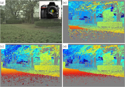
Figure 2a shows the change of the optical path through the lens with cyan and yellow color filters [Paramonov et al.(2016)Paramonov, Panchenko, Bucha, Drogolyub, and Zagoruyko, Moriuchi et al.(2017)Moriuchi, Sasaki, Mishima, and Mita]. The color direction of defocus blur with a near or far object is inverted at the focus distance. Such a change of the defocus blur allows retrieval of the distance in front of or behind the focal plane. Depth from defocus technique [Subbarao and Surya(1994)] is applied to estimate an accurate depth map for CCA [Martinello et al.(2015)Martinello, Wajs, Quan, Lee, Lim, Woo, Lee, Kim, and Lee, Moriuchi et al.(2017)Moriuchi, Sasaki, Mishima, and Mita], which is called depth from analytical defocus (DfAD). These methods assume the gaussian blur as shown in Figure 2c. The blur radius is estimated by , where and are deformed images by convolution kernels deforming the asymmetric gaussian blur of the R and B images to the gaussian blur of the G image and is zero-mean normalized cross correlation [Moriuchi et al.(2017)Moriuchi, Sasaki, Mishima, and Mita]. However, conventional CCA methods assume an ideal lens for simplifying analytical modeling of the defocus blur. By the difference between the analytical model and the actual one, as shown in Figure 3c, DfAD gives a distorted depth map due to a shift-variant PSF(Figure 2d). Figure 3f shows errors because of differences between the ideal analytical model and the actual one. Although recent work [Paramonov et al.(2016)Paramonov, Panchenko, Bucha, Drogolyub, and Zagoruyko] modeled the aberration effect by a double-Gauss lens model, the handcrafted model must be reconstructed when it is applied to other lenses.

3 Method
In this section, to overcome the differences between the analytical model and the actual one, we propose a physical cue-based deaberration network.
Baseline network We adopt patch-based architecture [Zagoruyko and Komodakis(2015), Simo-Serra et al.(2015)Simo-Serra, Trulls, Ferraz, Kokkinos, Fua, and Moreno-Noguer, Zbontar and LeCun(2016), Luo et al.(2016)Luo, Schwing, and Urtasun, Bailer et al.(2016)Bailer, Varanasi, and Stricker, Bailer et al.(2018)Bailer, Habtegebrial, Stricker, et al.] for our network to learn only the defocus blur instead of the contextual information and train the network easily. The architecture takes a patch extracted from a captured image as an input and outputs a single depth value corresponding to the patch. Since this network does not access to information of neighbor patches, it does not learn the contextual information. Therefore, the learned network has high generalization performance. This network can be trained by patchwise images with flat depth data only. Such data can be collected easily by our training system (see Section 4.1).
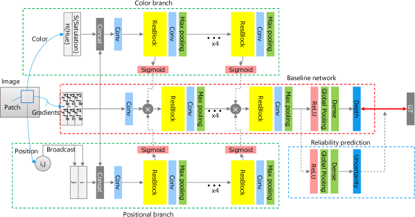
Our network structure is based on ResNet [He et al.(2016)He, Zhang, Ren, and Sun]. The baseline network structure is indicated by the red dotted rectangle in Figure 4. In a preprocessing stage, the gradient of an image patch is calculated with respect to the horizontal and vertical axis. All of the gradients are concatenated to . It is well known that gradients give better results than color images do [Bando et al.(2008)Bando, Chen, and Nishita, Chakrabarti and Zickler(2012), Martinello et al.(2015)Martinello, Wajs, Quan, Lee, Lim, Woo, Lee, Kim, and Lee, Paramonov et al.(2016)Paramonov, Panchenko, Bucha, Drogolyub, and Zagoruyko, Moriuchi et al.(2017)Moriuchi, Sasaki, Mishima, and Mita] and our experiment also has shown such result (see also Section 4.2). The gradients are processed by several ResBlocks, a convolution layer and max-pooling, followed by an activation function (ReLU) and global average pooling [Lin et al.(2013)Lin, Chen, and Yan] and a fully connected layer (dense layer). The network infers the defocus blur with learnable weight parameters as .
Deep deaberration network The aberration effect varies according to wavelength of color, horizontal and vertical axis in the lens. In order to handle the aberration effect, we add the positional and color information to the gradients as shown in Figure 4. The position is broadcasted into the same size as the patch. In order to add color information, the input image patch is converted to hue and saturation with the same shape of the patch.
In order to handle the lens aberration efficiently, we introduce the self-attention mechanism [Zhang et al.(2018)Zhang, Goodfellow, Metaxas, and Odena] to our deep deaberration network (DDN) indicated by the green dotted rectangle in Figure 4. Since the lens aberration causes the shape of the blur to change, important features vary according to the position of the image patch. The attention mechanism is trained so as to put large weights on such important features accordingly, and, thus, shift-invariant features are extracted as a result. The color branch can handle the dependency on object colors in the same way. After concatenating the positional and color information to the gradients, the attention maps are calculated by sigmoid functions from each feature map. The feature map of the main branch is multiplied by the above two attention maps before its ResBlock.
The proposed networks are trained as a regression problem with supervision similar to stereo matching [Kendall et al.(2017)Kendall, Martirosyan, Dasgupta, Henry, Kennedy, Bachrach, and Bry, Chang and Chen(2018)] and deep monocular depth estimation [Kuznietsov et al.(2017)Kuznietsov, Stückler, and Leibe, Atapour-Abarghouei and Breckon(2018)]. The ground truth distance recorded by the training system is converted to the blur radius by using the lens maker’s formula. A tuple of is the element of a training data-set, where is the index. L1 loss function is defined as where is the total number of the training patches.
Reliability prediction In actual CCA optics, the depth cues often disappear because of several uncertainties, such as saturation, soft shadow, dark color, and large blur. In the literature of Bayesian deep learning [Gal and Ghahramani(2016), Kendall and Gal(2017)], such uncertainties are categorized as heteroscedastic uncertainty [Kendall and Gal(2017)]. To handle the heteroscedastic uncertainty, the network should be changed to also output variance prediction as . The loss function is defined as heteroscedastic variance [Kendall and Gal(2017)]. However, this loss function shows significant instability in the training of our task as shown in Figure 8 (indicated by Bayes L2). This instability often causes training to fail. The progress of the training makes the variance prediction noticeably smaller and the error is also expected to be small. However, outlier errors make the loss very high because the denominator becomes very small simultaneously. Then, the loss function will diverge with the second order.
To stabilize the training, we propose a new loss function that has the heteroscedastic absolute standard deviation. In order to reduce the order, we convert the loss function by replacing the squared error and the variance with the absolute error and the absolute standard deviation as follows.
| (1) |
To output , an additional final layer is added to the end of the main branch in DDN indicated by the blue dotted rectangle in Figure 4. We use as the reliability. Figure 8 shows that our new loss function stabilizes the training significantly (indicated by Bayes L1).
4 Experiments

4.1 Training system, data and details
Training system We have developed a training system in order to automatically take many pictures with actual lenses as shown in Figure 5. This system consists of four 8K displays (LC-70X500) and a 12[m] slide stage arranged orthogonally to the displays. As these four displays are arranged 2 x 2, the screen size and resolution become 140 inches and 15360 x 8640, respectively. In order to learn only defocus blur information instead of contextual one, we introduce various randomization techniques to our training recipe to make the deep network focus on the blur information. We use many images sampled randomly from the MSCOCO data-set [Vinyals et al.(2017)Vinyals, Toshev, Bengio, and Erhan]. They are arranged in a matrix form as shown in Figure 5. Horizontal/vertical flipping and random scaling are applied to each image to remove its shape and scale information.
Training data We used a digital single-lens reflex (DSLR) camera: Nikon AI AF Nikkor 50mm f/1.8D (lens), Nikon D810 (body). The f-number was set to 4.0 throughout all experiments. The focus distance was set to 1500[mm] and the images were taken at 100 positions spaced at regular intervals on the blurred space from 1100[mm] to 2400[mm]. Four different images were taken at each position. Three images were for the training data and the last one was for the test data. This process took about only three hours. The captured images were resized to 1845x1232. We randomly collected image patches from only an edge and texture region without overlapping. The training and test data-sets include around 150,000 and 15,000 patches, respectively.
Implementation and training details Our DDN operates on an input patch size of 16x16 pixels with five Resblocks for each branch. The convolutional layers in all of our networks have 3x3 kernels and 1 stride. The number of channels is fixed to 32 from the beginning to the end. To train our networks, we use ADAM [Kingma and Ba(2014)] with the default parameters and 128 as the batch size. Although several data augmentation techniques [Krizhevsky et al.(2012)Krizhevsky, Sutskever, and Hinton] are usually applied in order to avoid overfitting, these techniques deform the shape of PSF which we should learn. We only select random crop [Buslaev et al.(2018)Buslaev, Parinov, Khvedchenya, Iglovikov, and Kalinin], brightness [Buslaev et al.(2018)Buslaev, Parinov, Khvedchenya, Iglovikov, and Kalinin] and random erasing [Zhong et al.(2017)Zhong, Zheng, Kang, Li, and Yang] that do not affect PSF. We trained DDN by 1500 epochs with the above training data and our training recipe. Finally, the test accuracy reached to 0.72 (=8.1[mm] at 1500[mm]).
4.2 Verifications
![[Uncaptioned image]](/html/1908.00329/assets/x5.png)
![[Uncaptioned image]](/html/1908.00329/assets/x6.png)
![[Uncaptioned image]](/html/1908.00329/assets/x7.png)
|
Ablation study We show the contributions of the proposed components by ablation study. Test accuracy curves during the training for the ablation study is shown in Figure 8. The result shows that the positional branch significantly affects accuracy. The Bayes L1 loss and the color branch have an effect on the accuracy. The gradient affects the accuracy slightly.
Effectiveness of positional branch We trained and tested the network with and without the positional branch using images having several sizes and shapes composed of several blocks as shown in Figure 10. In a large area, the training becomes hard because of the need to handle the shift-variant PSF. Figure 10 shows that the accuracy without the positional branch drops quickly as the area becomes large. As shown in Figure 11b, the distortion by the shift-variant PSF remains. In contrast, with the positional branch, the accuracy keeps high and the above distortion is disappeared in that depth map as shown in Figure 11d.
![[Uncaptioned image]](/html/1908.00329/assets/x8.png)
![[Uncaptioned image]](/html/1908.00329/assets/x9.png)
|

Effectiveness of color branch We evaluate the network with and without the color branch with respect to black-and-white and color subjects as shown in Figure 10. For the black-and-white subject, two networks have the same accuracy. The accuracy drops in the color subject because high saturated color confuses the network. Since the color branch helps the network to discriminate between the defocus blur and high saturated color, the color branch achieves higher accuracy. This is also shown in the depth maps as shown in Figure 11g and h.
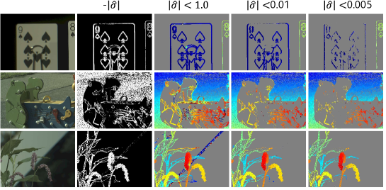
Effectiveness of reliability In actual scenes, we verify the effectiveness of the learned reliability. Figure 12 shows several samples of uncertainty. Several types of uncertainty caused depth errors. The reliability prediction can capture the depth errors correctly even though all of them are unseen for the learned network. Threshold shows good balance between the reliable and unreliable regions.
4.3 Quantitative and qualitative results
In the quantitative and qualitative experiments, the DDN is trained by only the indoor data-set. After the training, we changed the focus distance from 1500[mm] to 7000[mm] to apply it to outdoor scenes. We compared our DDN with DfAD [Moriuchi et al.(2017)Moriuchi, Sasaki, Mishima, and Mita] and a stereo camera composed of two prototype CCA cameras with 20cm baseline. Since DfAD utilizes DFD technique to the color channels, the comparison with DfAD includes the one with typical DFDs. Coded-aperture (CA) [Levin et al.(2007)Levin, Fergus, Durand, and Freeman] and focal track (FT) [Guo et al.(2017)Guo, Alexander, and Zickler] have some relations to our method but it is difficult to apply them to our CCA by the following reasons. The image of CCA has fewer zeros on the frequency domain than the requirement of CA. FT is based on the time derivative of defocus blur pairs by the small oscillation lens. It cannot be applicable to CCA due to large differences of blur between the inter-color channels.
Quantitative evaluation We quantitatively evaluated depth errors using our training system. To get stereo depth, we used semi-global matching (SGM) [Hirschmuller(2005)] implemented by [ope()]. Although SGM uses strong spatial regularization, DDN and DfAD don’t use it. This quantitative evaluation was set to the range from 2000 [mm] to 12000 [mm], which is different from the training. Figure 8 shows the error curves over the target distance. The error of DDN is much less than that of DfAD. The error of DDN falls short of the one of the stereo camera. However, the theoretical accuracy of our CCA camera is equivalent to the stereo camera with 1.25cm baseline according to the aperture size. Considering the aperture size, the accuracy of DDN is sufficiently high.
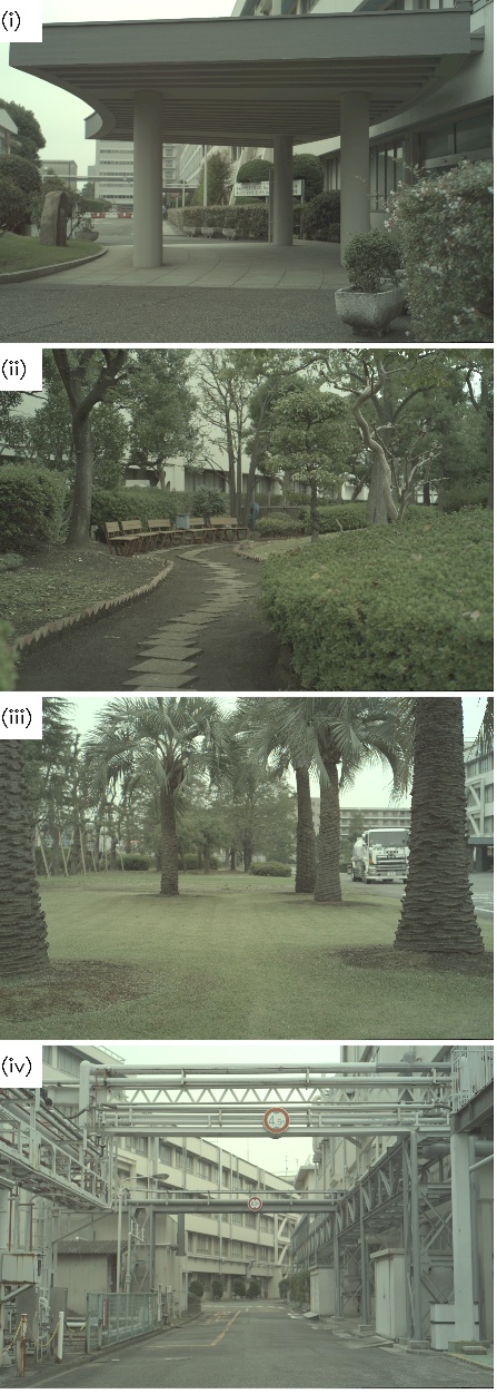
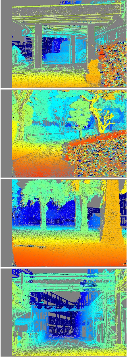
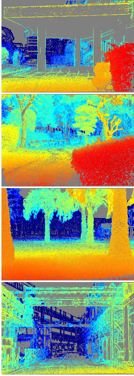
Qualitative evaluation We qualitatively evaluated the depth maps in actual outdoor scenes. Figure 13 shows the qualitative results. Gray color indicates that there is no depth cue. Depth maps by the stereo camera are high resolution at a great distance. However, depth errors often occur at a small distance (within 3[m]) as shown in (i) and (ii). They are caused by occlusion(iii). This is a problem specific to stereo matching. DfAD has insufficient resolution in the distant region((i), (ii), (iii) and (iv)). It also shows several errors caused by horizontal edges((i) and (iv)) and slant edges((iv)). In contrast, DDN gives improved depth maps for the failure cases both of the stereo camera and DfAD.
Robustness against to individual difference and other focal lengths For verification of the robustness against the individual difference, we also trained DDN by Lens B and C (Nikon AI AF Nikkor 50mm f/1.8D). We apply this trained DDNs to the captured image by Lens A (Nikon AI AF Nikkor 50mm f/1.8D) as shown in Figure 14. There is almost no difference in those depth maps. We also apply our method to f=14mm lens (AI AF Nikkor 14mm f/2.8D ED) and f=150mm lens (SP 150-600mm F/5-6.3 Di VC USD G2). As shown in Figure 15, DDN gives clear depth maps to not only f=50mm lens but also f=14mm lens and f=150mm lens.
5 Conclusion
With a view to realizing the single-shot depth measurement of a monocular camera, we have improved the depth measurement of CCA by using deep learning. We have proposed DDN with a self-attention mechanism to learn lens aberration efficiently. We have also proposed a Bayes L1 loss function to handle the uncertainty more accurately. We have confirmed that DDN showed a great advantage over the baseline in terms of accuracy and, in addition, the accuracy of Bayes L1 loss has been better than L1 loss. The learned reliability has been able to capture the errors caused by uncertainty correctly in spite of unseen outdoor scenes. In terms of quantitative results, the error of DDN was significantly better than DfAD. In terms of qualitative results, DDN was superior to DfAD for various outdoor scenes.


References
- [ope()] OpenCV. https://opencv.org/.
- [Agarwal et al.(2009)Agarwal, Snavely, Simon, Seitz, and Szeliski] Sameer Agarwal, Noah Snavely, Ian Simon, Steven M Seitz, and Richard Szeliski. Building rome in a day. In Computer Vision, 2009 IEEE 12th International Conference on, pages 72–79. IEEE, 2009.
- [Atapour-Abarghouei and Breckon(2018)] Amir Atapour-Abarghouei and Toby P. Breckon. Real-time monocular depth estimation using synthetic data with domain adaptation via image style transfer. In The IEEE Conference on Computer Vision and Pattern Recognition (CVPR), June 2018.
- [Bailer et al.(2016)Bailer, Varanasi, and Stricker] Christian Bailer, Kiran Varanasi, and Didier Stricker. Cnn based patch matching for optical flow with thresholded hinge loss. arXiv preprint arXiv:1607.08064, 2016.
- [Bailer et al.(2018)Bailer, Habtegebrial, Stricker, et al.] Christian Bailer, Tewodros Habtegebrial, Didier Stricker, et al. Fast feature extraction with cnns with pooling layers. arXiv preprint arXiv:1805.03096, 2018.
- [Bando et al.(2008)Bando, Chen, and Nishita] Yosuke Bando, Bing-Yu Chen, and Tomoyuki Nishita. Extracting depth and matte using a color-filtered aperture. ACM Transactions on Graphics (TOG), 27(5):134, 2008.
- [Buslaev et al.(2018)Buslaev, Parinov, Khvedchenya, Iglovikov, and Kalinin] Alexander Buslaev, Alex Parinov, Eugene Khvedchenya, Vladimir I Iglovikov, and Alexandr A Kalinin. Albumentations: fast and flexible image augmentations. arXiv preprint arXiv:1809.06839, 2018.
- [Chakrabarti and Zickler(2012)] Ayan Chakrabarti and Todd Zickler. Depth and deblurring from a spectrally-varying depth-of-field. In European Conference on Computer Vision, pages 648–661. Springer, 2012.
- [Chang and Chen(2018)] Jia-Ren Chang and Yong-Sheng Chen. Pyramid stereo matching network. In Proceedings of the IEEE Conference on Computer Vision and Pattern Recognition, pages 5410–5418, 2018.
- [Eigen et al.(2014)Eigen, Puhrsch, and Fergus] David Eigen, Christian Puhrsch, and Rob Fergus. Depth map prediction from a single image using a multi-scale deep network. In Advances in neural information processing systems, pages 2366–2374, 2014.
- [Fu et al.(2018)Fu, Gong, Wang, Batmanghelich, and Tao] Huan Fu, Mingming Gong, Chaohui Wang, Kayhan Batmanghelich, and Dacheng Tao. Deep ordinal regression network for monocular depth estimation. In Proceedings of the IEEE Conference on Computer Vision and Pattern Recognition, pages 2002–2011, 2018.
- [Gal and Ghahramani(2016)] Yarin Gal and Zoubin Ghahramani. Dropout as a bayesian approximation: Representing model uncertainty in deep learning. In international conference on machine learning, pages 1050–1059, 2016.
- [Godard et al.(2017)Godard, Mac Aodha, and Brostow] Clément Godard, Oisin Mac Aodha, and Gabriel J Brostow. Unsupervised monocular depth estimation with left-right consistency. In CVPR, volume 2, page 7, 2017.
- [Guo et al.(2017)Guo, Alexander, and Zickler] Qi Guo, Emma Alexander, and Todd Zickler. Focal track: Depth and accommodation with oscillating lens deformation. In Proceedings of the IEEE International Conference on Computer Vision, pages 966–974, 2017.
- [Haim et al.(2018)Haim, Elmalem, Giryes, Bronstein, and Marom] Harel Haim, Shay Elmalem, Raja Giryes, Alex M Bronstein, and Emanuel Marom. Depth estimation from a single image using deep learned phase coded mask. IEEE Transactions on Computational Imaging, 4(3):298–310, 2018.
- [He et al.(2016)He, Zhang, Ren, and Sun] Kaiming He, Xiangyu Zhang, Shaoqing Ren, and Jian Sun. Deep residual learning for image recognition. In Proceedings of the IEEE conference on computer vision and pattern recognition, pages 770–778, 2016.
- [Hirschmuller(2005)] Heiko Hirschmuller. Accurate and efficient stereo processing by semi-global matching and mutual information. In Computer Vision and Pattern Recognition, 2005. CVPR 2005. IEEE Computer Society Conference on, volume 2, pages 807–814. IEEE, 2005.
- [Kendall and Gal(2017)] Alex Kendall and Yarin Gal. What uncertainties do we need in bayesian deep learning for computer vision? In Advances in neural information processing systems, pages 5574–5584, 2017.
- [Kendall et al.(2017)Kendall, Martirosyan, Dasgupta, Henry, Kennedy, Bachrach, and Bry] Alex Kendall, Hayk Martirosyan, Saumitro Dasgupta, Peter Henry, Ryan Kennedy, Abraham Bachrach, and Adam Bry. End-to-end learning of geometry and context for deep stereo regression. CoRR, vol. abs/1703.04309, 2017.
- [Kim et al.(2012)Kim, Lee, Hayes, and Paik] Sangjin Kim, Eunsung Lee, Monson H Hayes, and Joonki Paik. Multifocusing and depth estimation using a color shift model-based computational camera. IEEE Transactions on Image Processing, 21(9):4152–4166, 2012.
- [Kingma and Ba(2014)] Diederik P Kingma and Jimmy Ba. Adam: A method for stochastic optimization. arXiv preprint arXiv:1412.6980, 2014.
- [Krizhevsky et al.(2012)Krizhevsky, Sutskever, and Hinton] Alex Krizhevsky, Ilya Sutskever, and Geoffrey E Hinton. Imagenet classification with deep convolutional neural networks. In Advances in neural information processing systems, pages 1097–1105, 2012.
- [Kuznietsov et al.(2017)Kuznietsov, Stückler, and Leibe] Yevhen Kuznietsov, Jörg Stückler, and Bastian Leibe. Semi-supervised deep learning for monocular depth map prediction. In Proc. of the IEEE Conference on Computer Vision and Pattern Recognition, pages 6647–6655, 2017.
- [Lee et al.(2013)Lee, Kim, Jung, Hayes, and Paik] Seungwon Lee, Nahyun Kim, Kyungwon Jung, Monson H Hayes, and Joonki Paik. Single image-based depth estimation using dual off-axis color filtered aperture camera. In Acoustics, Speech and Signal Processing (ICASSP), 2013 IEEE International Conference on, pages 2247–2251. IEEE, 2013.
- [Levin et al.(2007)Levin, Fergus, Durand, and Freeman] Anat Levin, Rob Fergus, Frédo Durand, and William T Freeman. Image and depth from a conventional camera with a coded aperture. ACM transactions on graphics (TOG), 26(3):70, 2007.
- [Lin et al.(2013)Lin, Chen, and Yan] Min Lin, Qiang Chen, and Shuicheng Yan. Network in network. arXiv preprint arXiv:1312.4400, 2013.
- [Luo et al.(2016)Luo, Schwing, and Urtasun] Wenjie Luo, Alexander G Schwing, and Raquel Urtasun. Efficient deep learning for stereo matching. In Proceedings of the IEEE Conference on Computer Vision and Pattern Recognition, pages 5695–5703, 2016.
- [Martinello et al.(2015)Martinello, Wajs, Quan, Lee, Lim, Woo, Lee, Kim, and Lee] Manuel Martinello, Andrew Wajs, Shuxue Quan, Hank Lee, Chien Lim, Taekun Woo, Wonho Lee, Sang-Sik Kim, and David Lee. Dual aperture photography: image and depth from a mobile camera. In Computational Photography (ICCP), 2015 IEEE International Conference on, pages 1–10. IEEE, 2015.
- [Moriuchi et al.(2017)Moriuchi, Sasaki, Mishima, and Mita] Yusuke Moriuchi, Takayuki Sasaki, Nao Mishima, and Takeshi Mita. 23-4: Invited paper: Depth from asymmetric defocus using color-filtered aperture. In SID Symposium Digest of Technical Papers, volume 48, pages 325–328. Wiley Online Library, 2017.
- [Paramonov et al.(2016)Paramonov, Panchenko, Bucha, Drogolyub, and Zagoruyko] Vladimir Paramonov, Ivan Panchenko, Victor Bucha, Andrey Drogolyub, and Sergey Zagoruyko. Depth camera based on color-coded aperture. In Proceedings of the IEEE Conference on Computer Vision and Pattern Recognition Workshops, pages 1–9, 2016.
- [Simo-Serra et al.(2015)Simo-Serra, Trulls, Ferraz, Kokkinos, Fua, and Moreno-Noguer] Edgar Simo-Serra, Eduard Trulls, Luis Ferraz, Iasonas Kokkinos, Pascal Fua, and Francesc Moreno-Noguer. Discriminative learning of deep convolutional feature point descriptors. In Proceedings of the IEEE International Conference on Computer Vision, pages 118–126, 2015.
- [Subbarao and Surya(1994)] Murali Subbarao and Gopal Surya. Depth from defocus: a spatial domain approach. International Journal of Computer Vision, 13(3):271–294, 1994.
- [Tang et al.(2017)Tang, Cohen, Price, Schiller, and Kutulakos] Huixuan Tang, Scott Cohen, Brian Price, Stephen Schiller, and Kiriakos N Kutulakos. Depth from defocus in the wild. In Proceedings of the IEEE Conference on Computer Vision and Pattern Recognition, pages 2740–2748, 2017.
- [Vinyals et al.(2017)Vinyals, Toshev, Bengio, and Erhan] Oriol Vinyals, Alexander Toshev, Samy Bengio, and Dumitru Erhan. Show and tell: Lessons learned from the 2015 mscoco image captioning challenge. IEEE transactions on pattern analysis and machine intelligence, 39(4):652–663, 2017.
- [Zagoruyko and Komodakis(2015)] Sergey Zagoruyko and Nikos Komodakis. Learning to compare image patches via convolutional neural networks. In Proceedings of the IEEE Conference on Computer Vision and Pattern Recognition, pages 4353–4361, 2015.
- [Zbontar and LeCun(2016)] Jure Zbontar and Yann LeCun. Stereo matching by training a convolutional neural network to compare image patches. Journal of Machine Learning Research, 17(1-32):2, 2016.
- [Zhang et al.(2018)Zhang, Goodfellow, Metaxas, and Odena] Han Zhang, Ian Goodfellow, Dimitris Metaxas, and Augustus Odena. Self-attention generative adversarial networks. arXiv preprint arXiv:1805.08318, 2018.
- [Zhong et al.(2017)Zhong, Zheng, Kang, Li, and Yang] Zhun Zhong, Liang Zheng, Guoliang Kang, Shaozi Li, and Yi Yang. Random erasing data augmentation. arXiv preprint arXiv:1708.04896, 2017.
- [Zhou and Nayar(2011)] Changyin Zhou and Shree K Nayar. Computational cameras: convergence of optics and processing. IEEE Transactions on Image Processing, 20(12):3322–3340, 2011.
