The ASAS-SN Catalog of Variable Stars V: Variables in the Southern Hemisphere

Abstract

The All-Sky Automated Survey for Supernovae (ASAS-SN) provides long baseline (${\sim}4$ yrs) light curves for sources brighter than V$\lesssim 17$ mag across the whole sky. As part of our effort to characterize the variability of all the stellar sources visible in ASAS-SN, we have produced ${\sim}30.1$ million V-band light curves for sources in the southern hemisphere using the APASS DR9 catalog as our input source list. We have systematically searched these sources for variability using a pipeline based on random forest classifiers. We have identified ${\sim}220,000$ variables, including ${\sim}88,300$ new discoveries. In particular, we have discovered ${\sim}48,000$ red pulsating variables, ${\sim}23,000$ eclipsing binaries, ${\sim}2,200$ $\delta$-Scuti variables and ${\sim}10,200$ rotational variables. The light curves and characteristics of the variables are all available through the ASAS-SN variable stars database (https://asas-sn.osu.edu/variables). The pre-computed ASAS-SN V-band light curves for all the ${\sim}30.1$ million sources are available through the ASAS-SN photometry database (https://asas-sn.osu.edu/photometry). This effort will be extended to provide ASAS-SN light curves for sources in the northern hemisphere and for V$\lesssim 17$ mag sources across the whole sky that are not included in APASS DR9.

1 Introduction

Recent large scale sky surveys such as the All-Sky Automated Survey (ASAS; Pojmanski 2002), the Optical Gravitational Lensing Experiment (OGLE; Udalski 2003),the Northern Sky Variability Survey (NSVS; Woźniak et al. 2004), MACHO (Alcock et al., 1997), EROS (Derue et al., 2002), the Catalina Real-Time Transient Survey (CRTS; Drake et al. 2014), the Asteroid Terrestrial-impact Last Alert System (ATLAS; Tonry et al. 2018a; Heinze et al. 2018), and Gaia (Gaia Collaboration et al., 2018a; Holl et al., 2018; Gaia Collaboration et al., 2018b) have revolutionized the study of stellar variability. Over time, these surveys have collectively discovered $\gtrsim 10^{6}$ variable stars across the whole sky.

Variable stars have been used to study astrophysics in multiple contexts. Pulsating variables, including Cepheids, RR Lyrae stars and Mira variables are used as distance indicators as they follow distinct period-luminosity relationships (e.g., Leavitt 1908; Matsunaga et al. 2006; Beaton et al. 2018; Whitelock et al. 2008, and references therein). Eclipsing binary stars are used to study stellar systems and with sufficient radial velocity followup, allow for the derivation of dynamical information and fundamental stellar parameters, including masses and radii of the stars in these systems (Torres et al., 2010). The precise measurements afforded by studying eclipsing binaries allow for the test of stellar theory across the Hertzsprung-Russell diagram. Variable stars are also used to study stellar populations and Galactic structure (Mateu, & Vivas, 2018; Matsunaga, 2018; Feast, & Whitelock, 2014).

The All-Sky Automated Survey for SuperNovae (ASAS-SN, Shappee et al. 2014; Kochanek et al. 2017) monitored the visible sky to a depth of $V\lesssim 17$ mag with a cadence of 2-3 days using two units in Chile and Hawaii each with 4 telescopes. ASAS-SN has recently expanded to 5 units with 20 telescopes. All the current ASAS-SN units are equipped with g-band filters and are currently monitoring the sky to a depth of $g\lesssim 18.5$ mag with a cadence of $\sim 1$ day. The ASAS-SN telescopes are hosted by the Las Cumbres Observatory (LCO; Brown et al. 2013) in Hawaii, Chile, Texas and South Africa. The primary focus of ASAS-SN is the detection of bright supernovae and other transients (e.g., tidal disruption events, cataclysmic variables, AGN flares, stellar flares, etc.) with minimal bias (e.g., Holoien et al. 2014, 2016, 2017, 2018a, 2018b), but its excellent baseline and all-sky coverage allows for the characterization of stellar variability across the whole sky.

In Paper I (Jayasinghe et al., 2018a), we discovered ${\sim}66,000$ new variables that were flagged during the search for supernovae, most of which are located in regions that were not well-sampled by previous surveys. In Paper II (Jayasinghe et al., 2019a), we homogeneously analyzed ${\sim}412,000$ known variables from the International Variable Stars Index (VSX,Watson et al. 2006), and developed a versatile random forest variability classifier utilizing the ASAS-SN V-band light curves and data from external catalogues. As data from The Transiting Exoplanet Survey Satellite (TESS; Ricker et al. 2015) became available, we have explored the synergy between the two surveys. The ASAS-SN light curves have long time baselines (${\gtrsim}4$ yr) and are sampled at a cadence of ${\sim}1-3$ days. Thus, these light curves complement the high cadence TESS light curves that have a shorter baseline. In Paper III (Jayasinghe et al., 2019b), we characterized the variability of ${\sim}1.3$ million sources within 18 deg of the Southern Ecliptic Pole towards the TESS continuous viewing zone and identified ${\sim}11,700$ variables, including ${\sim}7,000$ new discoveries. We also identified the most extreme heartbeat star system thus known, and characterized the system using both ASAS-SN and TESS light curves (Jayasinghe et al., 2018d). We have also explored the synergy between ASAS-SN and large scale spectroscopic surveys using data from APOGEE (Holtzman et al., 2015) with the discovery of the first likely non-interacting binary composed of a black hole with a field red giant (Thompson et al., 2018) and the identification of 1924 APOGEE stars as periodic variables in Paper IV (Pawlak et al., 2019). During our search for variables, we have also identified numerous unusual, rare variables, including 2 very long period detached eclipsing binaries (Jayasinghe et al., 2018b, c) and 19 R Coronae Borealis stars (Shields et al., 2018).

Here, we extracted the ASAS-SN light curves of ${\sim}30.1$ million sources from the AAVSO Photometric All-Sky Survey (APASS; Henden et al. 2015) DR9 catalog with $V<17$ mag in the southern hemisphere ($\delta<0$ deg). In this work, we systematically search this sample for variable sources. In Section $\S 2$, we discuss the input catalogue and the data reduction procedures used to obtain the ASAS-SN light curves. Section $\S 3$ discusses the random forest based variability identification and classification procedures. In Section $\S 4$, we discuss the ASAS-SN catalogue of variable stars in the southern hemisphere and present a summary of our work in Section $\S 5$.

2 Observations and Data reduction

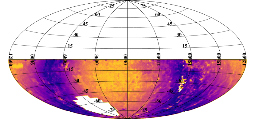
We started with the APASS DR9 catalog as our input source catalog. We chose the APASS catalog because the APASS survey had a faint completeness limit ($V\lesssim 16$) comparable to the ASAS-SN observations. We selected all the APASS sources with $V<17$ mag in the southern hemisphere ($\delta<0$ deg), excluding the ${\sim}1.3$M sources towards the Southern Ecliptic Pole which were analyzed in Paper III. This resulted in a list of ${\sim}30.1$M sources. Figure 1 illustrates the spatial distribution of these sources.

The ASAS-SN V-band observations used in this work were made by the “Brutus" (Haleakala, Hawaii) and “Cassius" (CTIO, Chile) quadruple telescopes between 2013 and 2018. Each ASAS-SN V-band field is observed to a depth of $V\lesssim 17$ mag. The field of view of an ASAS-SN camera is 4.5 deg², the pixel scale is 8$\aas@@fstack{\prime\prime}$0 and the FWHM is typically ${\sim}2$ pixels. ASAS-SN tends to saturate at ${\sim}10-11$ mag, but we attempt to correct the light curves of saturated sources for bleed trails (see Kochanek et al. 2017). The V-band light curves were extracted as described in Jayasinghe et al. (2018a) using image subtraction (Alard & Lupton, 1998; Alard, 2000) and aperture photometry on the subtracted images with a 2 pixel radius aperture. The APASS catalog was also used for calibration. We corrected the zero point offsets between the different cameras as described in Jayasinghe et al. (2018a). The photometric errors were recalculated as described in Jayasinghe et al. (2019b).

While we decided to use the APASS DR9 catalog as our input source list due to its all-sky coverage, this catalog has several shortcomings (Henden et al., 2015; Marrese et al., 2019). While the APASS DR9 sky coverage is nearly complete, there are regions towards the Galactic plane that are missing (see Figure 1). In addition, the DR9 catalog includes a number of duplicate entries, which appear to be caused by the merging process, where poor astrometry in a given field may cause two centroids to be included for a single source. Centroiding in crowded fields is also poor and blends cause both photometric and astrometric errors. The APASS DR9 catalog does not provide unique identifiers, thus we used the VizieR (Oelkers et al., 2018) recno field as unique identifiers. To address the issue of incomplete sky coverage we will use the ATLAS All-Sky Stellar Reference Catalog (Tonry et al., 2018b) in the next paper to produce light curves for the missing sources in APASS DR9.

Figure 1: Sky density plot of the ${\sim}30.1$M APASS DR9 sources analyzed in this work. Sources in the gap centered at the Southern Ecliptic Pole ($\alpha=6$ h, $\delta=-66.55$ deg) were analyzed in Jayasinghe et al. (2019b). The gaps near ($\alpha=18$ h, $\delta=-30$ deg) are in the input APASS DR9 catalog.

3 Variability Analysis

Here we describe the procedure we used to identify and characterize variables in the source list. We describe how we cross-matched the APASS sources to external catalogues in Section $\S 3.1$. In Section $\S 3.2$, we describe the procedure we took to identify candidate variable sources using a random forest classifier. In Section $\S 3.3$, we discuss the classification of the candidate variables into the various standard classes of variable stars using the V2 random forest classifier model from Jayasinghe et al. (2019a), in Section $\S 3.4$, we discuss our attempts to mitigate the effects of blending on the list of candidate variables and in Section $\S 3.5$, we discuss the quality checks that we used to improve the final variables catalog.

3.1 Cross-matches to external catalogs

We cross-match the APASS DR9 sources with Gaia DR2 (Gaia Collaboration et al., 2018a) using a matching radius of 5$\aas@@fstack{\prime\prime}$0. The sources were also cross-matched to the Gaia DR2 probabilistic distance estimates from Bailer-Jones et al. (2018). Even though we used a liberal matching radius, ${\sim}84\%$ (${\sim}94\%$) of the sources have a cross-match in Gaia DR2 within 2$\aas@@fstack{\prime\prime}$0 (3$\aas@@fstack{\prime\prime}$0). These sources were also cross-matched with the 2MASS (Skrutskie et al., 2006) and AllWISE (Cutri et al., 2013; Wright et al., 2010) catalogues using a matching radius of 10$\aas@@fstack{\prime\prime}$0. The cross-matches to these catalogues provide useful information that are later used in the identification and classification of variable stars. We used TOPCAT (Taylor, 2005) to cross-match the APASS sources with these external catalogues.

Sources in the Small Magellanic Cloud (SMC) are also included in our input source list. We used association information from Gaia DR2 (Gaia Collaboration et al., 2018c) to identify ${\sim}1,600$ sources from our source list that are SMC members. For sources in the SMC, we use a distance of $d=62.1$ kpc (Graczyk et al., 2014) in our variability classifier instead of the distance estimate from Bailer-Jones et al. (2018). The LMC was covered in Paper III.

3.2 Random Forest Variable Identification

In Paper III we used several methods, including linear cuts on Lomb-Scargle periodogram statistics, light curve features and external photometry to identify variable sources. Here, we take a different approach by training and apply a random forest classifier to distinguish candidate variables from constant sources. We built a variability classifier based on a random forest (RF) model using scikit-learn (Pedregosa et al., 2012; Breiman, 2001). A random forest classifier is an ensemble of decision trees whose output is the mean prediction of the individual decision trees (Breiman, 2001). The set of variable sources used to train this classifier consisted of ${\sim}302,000$ variables from Papers II and III with definite classifications. Variables with uncertain classifications, including ‘VAR’ and ‘ROT:’, were not included in this list as they reduced the accuracy of the final random forest classification model. The set of constant sources in the training list consisted of ${\sim}600,000$ sources randomly selected from the list of constant sources in Paper III.

The goal was to provide classifications into two broad groups: CONST (constant stars) and VAR (potential variables). The potential variables will be analyzed in further detail so it is more important not to lose real variables than to accidentally include non-variables. These broad classes were selected to reduce the complexity of the classifier, and to provide an accurate initial separation prior to reclassifying the variable sources with the random forest variable type classifier from Paper II. To generate periodicity statistics, we used the astropy implementation of the Generalized Lomb-Scargle (GLS, Zechmeister & Kürster 2009; Scargle 1982) periodogram to search for periodicity over the range $0.05\leq P\leq 1000$ days in all ${\sim}30.1$M light curves. The GLS periodogram is an extension of the standard Lomb-Scargle periodogram that uses a frequency dependent light curve mean,

$$y_{\rm model}(t;f)=y_{0}(f)+A_{f}\sin\big{(}2\pi f(t-\phi_{f})\big{)},$$

(eq. 41 from VanderPlas 2018). This floating-mean model is more robust if there are gaps in the phased data than the standard Lomb-Scargle periodogram (VanderPlas, 2018). We utilize the best GLS period, false alarm probability (FAP) and the power of the best GLS period as features. The best GLS period is defined to be the period with the largest power which is essentially a measure of the SNR of the periodogram peak. The false alarm probability is the probability that a light curve with no signal would lead to a GLS peak of a similar magnitude (VanderPlas, 2018).

We further characterize the periodicity of the light curves using the Lafler-Kinmann string length statistic (Lafler & Kinman, 1965; Clarke, 2002). We use the definition

$$T(\phi|P)=\frac{\sum_{i=1}^{\rm N}(m_{i+1}-m_{i})^{2}}{\sum_{i=1}^{\rm N}(m_{i}-\overline{m})^{2}}\times\frac{(N-1)}{2N}$$ (1)

from Clarke (2002), where the $m_{i}$ are the magnitudes sorted by phase and $\overline{m}$ is the mean magnitude. We also calculate the statistic $T(t)$ after sorting the light curve by time instead of phase. The complete list of 20 features and their importances to the trained random forest model is summarized in Table 1. Feature importances are calculated as Gini importances using the mean decrease impurity algorithm (Pedregosa et al., 2012).

The overall results of the random forest model are evaluated based on the

$$\rm precision=\frac{\alpha}{\alpha+\beta}\,,$$ (2)

$$\rm recall=\frac{\alpha}{\alpha+\gamma}\,,$$ (3)

and the harmonic mean of the two,

$$F_{1}=2\bigg{(}\frac{\rm precision\times\rm recall}{\rm precision+\rm recall}\,\bigg{)},$$ (4)

where $\alpha$, $\beta$ and $\gamma$ are the number of true positives, false positives and false negatives in a given class respectively. These quantities are evaluated for both the constant (CONST) and variable (VAR) sources (Table 2).

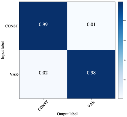
The parameters of the random forest model were optimized using cross-validation to maximize the overall $F_{1}$ score of the classifier. The number of decision trees in the forest was initialized to n_estimators=1000. We also limited the maximum depth of the decision trees to max_depth=16 in order to mitigate over-fitting, set the number of samples needed to split a node as min_samples_split=10 and set the number of samples at a leaf node as min_samples_leaf=5. To further minimize over-fitting, we also assigned weights to each class with class_weight=‘balanced_subsample’. For any given source, the RF classifier assigns classification probabilities $\rm Prob(Const)$ and $\rm Prob(Var)=1-Prob(Const)$. The output classification of the RF classifier is the class with the highest probability. We split the training sample for training ($80\%$) and testing ($20\%$) in order to evaluate the performance of the RF classifier. The confusion matrix for the trained RF model is shown in Figure 2. The greatest confusion (2%) arises from input variable sources that are subsequently classified as constant stars. The performance of the classifier is summarized in Table 2. The overall $F_{1}$ score for the classifier is 98.5%.

We further investigate the performance variation of the RF classifier with magnitude by binning the test sample by the median V-band magnitude (Table 3). The $F_{1}$ score for the classifier is lowest ($92.9\%$) for sources with $V\leq 11$ mag where 15% of the input constant sources are incorrectly classified as variable sources. This is likely due to saturation artifacts that arise at these bright magnitudes. The $F_{1}$ score varies by $<1\%$ between $11<V\leq 17$ mag and the confusion between constant and variables sources is also minimal. Most of the sources ($96.3\%$) in the test sample have median magnitudes that fall within this range. For sources at the ASAS-SN V-band faint limit of $V\geq 17$ mag, the $F_{1}$ score drops to $95.5\%$ and the confusion between classes again rises. This is not surprising as at these magnitudes the light curves are dominated by noise.

Figure 2: The normalized confusion matrix derived from the final version of the trained random forest classifier. The y-axis corresponds to the ‘input’ classification, while the x-axis is the ‘output’ prediction obtained from the trained random forest model.

Table 1: Variability features and their importances for variable star identification

Feature	Description	Importance	Reference
LS_Per	Best Lomb-Scargle period	1%	-
LS_Pow	Power corresponding to the best Lomb-Scargle period	24%	-
log(LS_FAP)	Base 10 logarithm of the False Alarm Probability corresponding to the best Lomb-Scargle period	11%	-
$\rm T(t)$	Lafler-Kinman String Length statistic of the light curve sorted by time	4%	Jayasinghe et al. (2019a)
$\rm T(\phi|P)$	Lafler-Kinman String Length statistic of the light curve sorted by phase	18%	Jayasinghe et al. (2019a)
$\delta$	Normalized difference between $\rm T(t)$ and $\rm T(\phi|P)$	5%	Jayasinghe et al. (2019b)
$\rm Skew$	Skewness of the magnitude distribution	2%	-
$\rm Kurt$	Kurtosis of the magnitude distribution	2%	-
$\rm Median$	Median of the magnitude distribution	1%	-
$\sigma$	Standard deviation of the light curve	2%	-
IQR	Difference between the 75th and 25th percentiles in magnitude	2%	-
$A_{\rm HL}$	Ratio of magnitudes brighter or fainter than the average	2%	Kim & Bailer-Jones (2016)
$\rm MAD$	Median absolute deviation of the light curve	2%	-
$1/\eta$	Inverse of the $\eta$ (Von Neumann index) value for the light curve	3%	Von Neumann et al. (1941)
$J-K_{s}$	2MASS $J-K_{s}$ color	12%	Skrutskie et al. (2006)
$H-K_{s}$	2MASS $H-K_{s}$ color	9%	Skrutskie et al. (2006)

Table 2: Overall performance of the ASAS-SN random forest source classifier

Class	Precision	Recall	$F_{1}$ score	Sources
CONST	99$\%$	99$\%$	99$\%$	600,000
VAR	98$\%$	98$\%$	98$\%$	302,021

Table 3: Performance of the ASAS-SN random forest source classifier with magnitude

Median magnitude	$F_{1}$ score	Constant Star False Positive Rate	Variable Star False Positive Rate	Sources (%)
$V\leq 11$ mag	92.9$\%$	15$\%$	2$\%$	3.1%
$11<V\leq 13$ mag	98.5$\%$	1$\%$	2$\%$	11.5%
$13<V\leq 15$ mag	98.9$\%$	1$\%$	1$\%$	37.5%
$15<V\leq 17$ mag	98.4$\%$	1$\%$	3$\%$	47.3%
$V\geq 17$ mag	95.5$\%$	5$\%$	4$\%$	0.8%

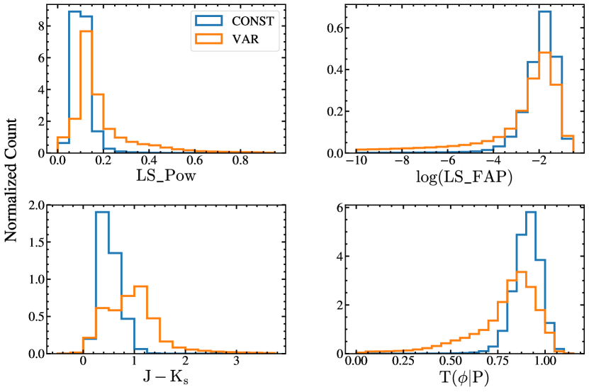
We applied the trained random forest classifier to the entire sample of ${\sim}30.1$M sources and identified 3,553,235 candidate variables. The distinction between the constant sources and the candidate variables is illustrated in Figure 3 through the distributions of the four features with the largest importance: LS_Pow, $\rm T(\phi|P)$, $J-K_{s}$ and log(LS_FAP). We find that many candidate variable sources are strongly periodic with high values of LS_Pow and smaller values of log(LS_FAP) and $\rm T(\phi|P)$. In addition, the distribution of the 2MASS color $J-K_{s}$ differs significantly between constant and variable sources. Variable sources are skewed towards redder near-infrared colors with $J-K_{s}>1$ mag while constant sources largely peak around $J-K_{s}\sim 0.5$ mag. Cooler, evolved stars are more likely to be variable, so this is not unexpected. Nevertheless, the distributions of constant and variable sources overlap significantly in the feature spaces illustrated in Figure 3. It is crucial to note that while we illustrated these distributions linearly, the RF classifier is inherently non-linear and relies on a complex ensemble of decision trees to predict the class of any given source. In this sense, even the features with the least importance do matter for the overall success of the classifications.

Figure 3: Distribution of the sources classified as CONST and VAR in the LS_Pow, $\rm T(\phi|P)$, $J-K_{s}$ and log(LS_FAP) features. Sources with log(LS_FAP)$<-10$ are not shown for clarity.

3.3 Variability Classification

Once candidate variables are identified, we aimed at classifying these sources into the various standard classes of variable stars. We use the variability classifier implemented in Jayasinghe et al. (2019a), which consists of a random forest classifier plus several refinement steps. Given the large number of candidates, we changed our variability classification strategy as follows.

• Initially, we classified all the candidate variables using just the GLS periods derived in $\S 3.2$.

• Following this, we derive periods for a limited set of sources (see below) using the astrobase implementation (Bhatti et al., 2018) of the Box Least Squares (BLS, Kovács et al. 2002) periodogram to improve the completeness for eclipsing binaries whose periodicity cannot be easily identified with GLS.

We also run the variability classifier twice, once using the best period (GLS or BLS) and once using twice the best period. The final classification is the one which yields the greatest classification probability. This step greatly improves the separation of EW type eclipsing binaries from RRC variables, and also improves upon the efficiency of the automated period doubling algorithm that was used for eclipsing binaries in Paper II.

To identify possible eclipsing binaries, we selected ${\sim}576,000$ candidate variables with $A_{\rm HL}>2$ (Table 1) from our original list. $A_{\rm HL}$ is the ratio of magnitudes brighter or fainter than the average magnitude (Kim & Bailer-Jones, 2016). Since eclipses usually only span limited phase ranges, $A_{\rm HL}$ tends to be higher for the light curves of eclipsing binaries compared to other variable types. We searched for periods over the range $0.05\leq P\leq 1000$ days and the BLS periodogram was initialized with 200 phase bins and a minimum (maximum) transit duration of $0.1$ $(0.3)$ in phase. BLS periods were only selected if the BLS power was $<0.3$. We identified ${\sim}3,500$ eclipsing binaries through this process.

3.4 Blending Corrections

Blending towards crowded regions (e.g., the Galactic disk) is problematic owing to the large pixel scale (8$\aas@@fstack{\prime\prime}$0) and the FWHM (${\sim}$16$\aas@@fstack{\prime\prime}$0) of the ASAS-SN images. The APASS data has a significantly smaller pixel scale (2$\aas@@fstack{\prime\prime}$6), so we can have multiple APASS sources inside a single ASAS-SN resolution element. To minimize the number of false positives in our catalogue of variables due to blending, we identify and correct blended variable groups in our catalog. However, we have not attempted to correct for the contaminating light in the photometry of the blended sources.

We find that ${\sim}1.1$M of the ${\sim}3.6$M candidate variables had at least one neighbor within 30$\aas@@fstack{\prime\prime}$0 from their positions. For these sources, we compute the flux variability amplitudes using a non-parametric random forest regression model (Jayasinghe et al., 2019a). We then identify groups of blended variables based on the cross-matching. For each blended variable group, we select the source with the largest flux variability as the ‘true’ variable, and discard the remaining overlapping sources in the blended group from the final list. After removing these overlapping, blended sources from the list of candidate variables, we were left with ${\sim}3$M sources.

3.5 Quality Checks

At this stage, visual review of a random set of light curves suggested that quality checks must be implemented to distinguish true variability signals from variability due to bad photometry, and other survey specific issues (e.g., shutter failures, etc.). In Paper III, given the significantly shorter list of candidate variables, this was accomplished through simple visual review of the light curves. In this work, given the shear number of sources, visual review is not a feasible option. Thus, we choose to implement various criteria in lieu of visual review, to distinguish the true variables from the ‘noise’.

We first restrict the list to sources with $\rm V_{mean}>10$ mag, $A>0.05$ mag and $\rm T(t)<0.9$. We implemented the cut in the ASAS-SN V-band magnitude to minimize noise due to saturation artifacts. We also calculate the ratio between the amplitude estimated by random forest regression ($A$) to the interquartile range IQR (Table 1) of the light curve,

$$\alpha=A/\rm IQR\,,$$ (5)

and the absolute, reddening-free Wesenheit magnitudes (Madore, 1982; Lebzelter et al., 2018)

$$W_{RP}=M_{\rm G_{RP}}-1.3(G_{BP}-G_{RP})\,,$$ (6)

and

$$W_{JK}=M_{\rm K_{s}}-0.686(J-K_{s})\,,$$ (7)

for each source, where the $G_{BP}$ and $G_{RP}$ magnitudes are from Gaia DR2 (Gaia Collaboration et al., 2018a) and the $J$ and $K_{s}$ magnitudes are from 2MASS (Skrutskie et al., 2006). The Wesenheit magnitudes are used in the pipeline from paper II to refine variable type classifications. The quantity $\alpha$ can be used to identify light curves with significant outliers as we expect $\alpha\approx 2$ for most sources.

The criteria used in lieu of visual review are summarized in Table 4. We note that these criteria are applied in addition to the refinement criteria in Paper II. These are not replacements but additional quality checks intended to improve the purity of our catalog. We derived these criteria through visual inspection in order to minimize false positives in the different variable groups. In addition to the criteria summarized in Table 4, we further scrutinize sources with periods that are close to aliases of a sidereal day (e.g., $P\approx 1$ d, $P\approx 2$ d, $P\approx 30$ d, etc.). This is accomplished by tightening the criteria on $\rm T(\phi|P)$, log(LS_FAP), LS_Pow and $\delta$. This process slightly reduces the completeness of our catalog at these periods, but greatly reduces the number of false positives. In addition, we removed QSO contaminants in this list by cross-matching our list of variables to the Liao et al. (2019) catalog of known QSOs using a matching radius of 5$\aas@@fstack{\prime\prime}$0. We identified 336 cross-matches, out of which 325 were classified as YSO variables in our pipeline. At this point we had ${\sim}247,200$ sources nominally classified as variable stars.

We inspected 5000 randomly selected sources classified as non-variable and the same number classified as variable. This was partly just a sanity check but also driven by the concern that the large size of our initial list (${\sim}10\%$ of the sources) suggested that our false positive rates had to be higher than suggested by Table 2. Among the non-variable sources, we identified only 3 ($\sim 0.06\%$) that might be low level variables, which suggests that we are missing few variables that can be detected in this data. For the variable stars, we found significant numbers of false positives in the following variable classes: GCAS (${\sim}50\%$), L (${\sim}25\%$), VAR (${\sim}45\%$) and YSO (${\sim}13\%$). The implied false positive rate for the variable sources was ${\sim}5.9\%$ at this point.

Light curves that are contaminated by systematics tend to be classified as irregular or generic variables as they are inherently aperiodic in nature. Thus, we decided to review all ${\sim}32,800$ sources that were classified as L, VAR, GCAS, or YSO to improve the purity of our catalog. Initial results suggested that L variables with $T(t)>0.65$ were dominated by noise, so we rejected ${\sim}14,300$ such sources without further visual review. We visually reviewed the remaining ${\sim}18,500$ sources, and rejected ${\sim}12,600$ sources (${\sim}68\%$) and only retained ${\sim}5,900$ of these sources in the final catalog. When we carried out a new inspection of 5000 randomly selected variables, the false positive rates were now EA (${\sim}1.4\%$), L (${\sim}0.6\%$), SR (${\sim}2.6\%$), and VAR (${\sim}0.9\%$). This implies an overall false positive rate for the final catalog of variable sources of $\sim 1.3\%$.

After these criteria are applied, we end up with a list of ${\sim}220,000$ variables. This means that our initial candidate list had a false positive rate of ${\sim}93\%$. The larger than expected false positive rate is partly due to a biased training set in the source classifier. The training set of constant sources was derived from a region of the sky away from the Galactic plane. The increased crowding and blending towards the Galactic plane will systematically affect constant stars at low latitudes and introduce spurious variability signals into their light curves. Our classifier will identify these constant sources as candidate variables. In addition to this, sources in the vicinity of bright, saturated stars in our data are likely to have spurious variability signals in their image subtraction light curves due to the corrections made for bleed trails (see Kochanek et al. 2017). This effect is again exacerbated towards the Galactic plane.

Table 4: Summary of the variability refinement criteria for each variable class.

Class	Summarized refinement Criteria
$\delta$ Scuti (HADS, DSCT)
	$\rm Skew<0.15$, LS_Pow>0.25, log(LS_FAP)$<-7$, $A<0.5$ mag, $\rm T(\phi|P)<0.5$, $-1<W_{JK}<3$ mag
RR Lyrae (RRAB, RRC, RRD)
	RRAB and log(LS_FAP)$<-10$, LS_Pow>0.2, $A>0.08$ mag, $\rm T(\phi|P)<0.6$, $\rm Skew<0.15$, $\delta<-0.25$
	RRC/RRD and log(LS_FAP)$<-10$, LS_Pow>0.2, $A>0.08$ mag, $\rm T(\phi|P)<0.6$, $\rm Skew<0$, $\delta<-0.25$
Cepheids (DCEP, DCEPS, CWA, CWB, RVA)
	$\rm Skew<1$, log(LS_FAP)$<-10$, LS_Pow>0.3, $A<2$ mag, $\rm T(\phi|P)<0.6$, $\delta<-0.25$
Rotational Variables (ROT)
	Period$>0.6$ d and log(LS_FAP)$<-5$, LS_Pow>0.2, $A>0.08$ mag, $\rm T(\phi|P)<0.6$, $\delta<0$
	Period$\leq 0.6$ d and $W_{JK}>2.5$ mag, $\rm Prob>0.9$
Eclipsing Binaries (EA, EB, EW)
	EA (GLS) and $\alpha<100$, $\rm T(\phi|P)<0.6$, $A>0.08$ mag
	EB (GLS) and log(LS_FAP)$<-7$, LS_Pow>0.2, $A>0.08$ mag, $\rm T(\phi|P)<0.6$
	EW (GLS) and log(LS_FAP)$<-7$, LS_Pow>0.2, $A>0.08$ mag, $\rm T(\phi|P)<0.6$, $\rm Skew>0$
	EA (BLS) and $\alpha<100$, $\rm T(\phi|P)<0.45$, $\rm Prob>0.8$
Semiregular and Irregular Variables (SR, L)
	$\alpha<5$, $\rm V_{mean}>11$ mag, $A>0.08$ mag
	Period$>100$ d and log(LS_FAP)$<-3$, $J-K_{s}>1.1$, $A>0.1$ mag, $\rm T(t)<0.7$
	$10\leq$Period$\leq 100$ d and log(LS_FAP)$<-8$, $A>0.08$ mag
Mira Variables (M, M:)
	log(LS_FAP)$<-3$, LS_Pow>0.5 , $\rm T(\phi|P)<0.5$
Young Stellar Objects (YSO)
	Period$<100$ d and $\alpha<5$, log(LS_FAP)$<-10$, LS_Pow>0.25, $\rm T(\phi|P)<0.6$
Outbursting Be stars (GCAS, GCAS:)
	$\alpha<5$, $\rm V_{mean}>11$ mag, $J-K_{s}<1.1$, $0.25<A<1$ mag, $\rm T(t)<0.5$
Generic Variables (VAR)
	$\alpha<5$, $0.1<A<2$ mag, $W_{JK}>-4$ mag, $\rm V_{mean}>11$ mag, $\rm T(\phi|P)<0.5$ OR $\rm T(t)<0.5$

4 Results

The complete catalog of ${\sim}220,000$ variables and their light curves are available at the ASAS-SN Variable Stars Database (https://asas-sn.osu.edu/variables) along with the V-band light curves for each source. Most of the known variables identified in this work were already added to the Variable Stars Database in Paper II. We have overhauled the web interface for the ASAS-SN Variable Stars Database to include interactive light curve plotting and photometry from Gaia DR2, APASS DR9, 2MASS and ALLWISE. Table 5 lists the number of sources of each variability type in the catalog.

In order to identify known variable stars, we matched our list of variables to the VSX (Watson et al., 2006) catalog, with a matching radius of 16$\aas@@fstack{\prime\prime}$0. The variables discovered by the All-Sky Automated Survey (ASAS; Pojmanski 2002) and the Catalina Real-Time Transient Survey (CRTS; Drake et al. 2014) have already been incorporated into the VSX database. Numerous other studies (e.g., Mateu et al. 2012; Fernández-Trincado et al. 2015 and references therein) have also searched for variable stars on a smaller scale (e.g., globular clusters). While some of these results have been included in the VSX catalog, we note that the inclusion of these studies in the VSX catalog is likely to be incomplete. We also match our variables to the catalog of variable stars discovered by ASAS-SN (Jayasinghe et al., 2018a), the catalogs of variable stars in the Magellanic clouds and the Galactic bulge from the Optical Gravitational Lensing Experiment (OGLE; Udalski 2003; Pawlak et al. 2016; Soszyński et al. 2016; Udalski et al. 2018, and references therein), the catalog of variables from the Asteroid Terrestrial-impact Last Alert System (ATLAS; Tonry et al. 2018a; Heinze et al. 2018), the Gaia DR2 catalog of variables (Gaia Collaboration et al., 2018a; Holl et al., 2018; Gaia Collaboration et al., 2018b), the catalog of variables identified by KELT (Oelkers et al., 2018), the catalog of WISE variables (Chen et al., 2018) and the variables from MACHO (Alcock et al., 1997). Of the ${\sim}220,000$ variables identified in this work, ${\sim}131,900$ were previously discovered by other surveys, and ${\sim}88,300$ are new discoveries, as also listed in Table 5.

It is evident that previous surveys, including our discoveries from paper I, successfully discovered sources that have large amplitudes or are strongly periodic. Most (${\sim}54\%$) of our new discoveries are red, pulsating variables. We also discover a large number of binaries and rotational variables, amounting to ${\sim}26\%$ and ${\sim}12\%$ of the newly discovered variable sources, respectively. It is also noteworthy that we discover many more $\delta$ Scuti sources than previously known. These variables are particularly interesting as they pulsate at high frequencies (P$<0.3$ d) and are located towards the lower end of the instability strip (Breger, 1979). $\delta$ Scuti variables are also known to follow a period-luminosity relationship (Lopez de Coca et al., 1990).

Table 5: Variables by type

VSX Type	Description	Known	New
CWA	W Virginis type variables with $P>8$ d	205	51
CWB	W Virginis type variables with $P<8$ d	225	45
DCEP	Fundamental mode Classical Cepheids	645	16
DCEPS	First overtone Cepheids	171	9
DSCT	$\delta$ Scuti variables	744	1354
EA	Detached Algol-type binaries	11413	9948
EB	$\beta$ Lyrae-type binaries	8574	4115
EW	W Ursae Majoris type binaries	27926	8887
HADS	High amplitude $\delta$ Scuti variables	1338	849
M	Mira Variables	3472	38
ROT	Rotational variables	7200	10236
RRAB	RR Lyrae variables (Type ab)	12936	294
RRC	First Overtone RR Lyrae variables	2655	1015
RRD	Double Mode RR Lyrae variables	233	12
RVA	RV Tauri variables (Subtype A)	32	0
SR	Semi-regular variables	44198	45556
L	Irregular variables	4979	2528
GCAS	$\gamma$ Cassiopeiae variables	20	8
YSO	Young stellar objects	1949	980
GCAS:	Uncertain $\gamma$ Cassiopeiae variables	20	6
VAR	Generic variables	2789	2343

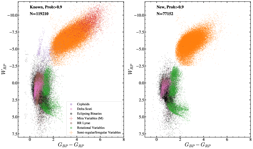
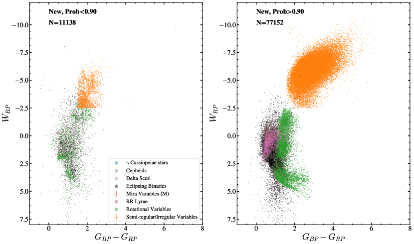
The Wesenheit $W_{RP}$ vs. $G_{BP}-G_{RP}$ color-magnitude diagram for all the variables with excellent variable type classification probabilities ($\rm Prob>0.9$) is shown in Figure 4. Generic and uncertain variable types are not shown. We have sorted the variables into groups to highlight the different classes of variable sources. A similar Wesenheit $W_{RP}$ vs. $G_{BP}-G_{RP}$ color-magnitude diagram for all the newly discovered variables, separated by probability, is shown in Figure 5. The sharp cutoffs seen in the sample of semi-regular variables with $\rm Prob<0.9$ are inherited from the variable type refinements from paper II. Most variables with $\rm Prob<0.9$ are located in similar areas of the CMD as the variables with $\rm Prob>0.9$. However, we note two interesting clusters of these low-probability variables at ($G_{BP}-G_{RP}$, $W_{RP}$) $\sim$ $(2.5,-4.5)$ and $(0.75,1.8)$ corresponding to semi-regular and rotational variables respectively. We plan to further investigate these clusters after the variable sources in the northern hemisphere have been incorporated into our catalog.

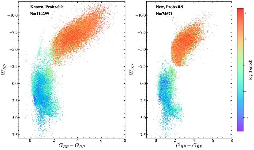
The Wesenheit $W_{RP}$ vs. $G_{BP}-G_{RP}$ color-magnitude diagram for all the variables with $\rm Prob>0.9$ and the points colored according to the period is shown in Figure 6. This essentially highlights the large dynamic range in period probed by the ASAS-SN light curves. Owing to the ASAS-SN survey cadence and our long time baseline, we are able to probe both short period variability ($P<0.1$ d) and long period variability ($P>1000$ d). The ASAS-SN survey continues to monitor the sky in the g-band, which lends itself well to the analysis of long term trends and unusual variability. As a testament to this, Jayasinghe et al. (2019c) noted a sudden dimming episode (flux reduction of ${\sim}70\%$ in the g-band) in an APASS source (ASASSN-V J213939.3$-$702817.4) that was non-variable for ${\sim}1800$ d. This source was classified as a constant source in this work.

Figure 4: The Wesenheit $W_{RP}$ vs. $G_{BP}-G_{RP}$ color-magnitude diagram for the variables with $\rm Prob>0.9$, that have already been discovered (left), and the new discoveries (right).

Figure 5: The Wesenheit $W_{RP}$ vs. $G_{BP}-G_{RP}$ color-magnitude diagram for the newly discovered variables with $\rm Prob<0.9$ (left), and $\rm Prob>0.9$ (right).

Figure 6: The Wesenheit $W_{RP}$ vs. $G_{BP}-G_{RP}$ color-magnitude diagram for the periodic variables with $\rm Prob>0.9$, that have already been discovered (left), and the new discoveries (right). The points are colored by the period.

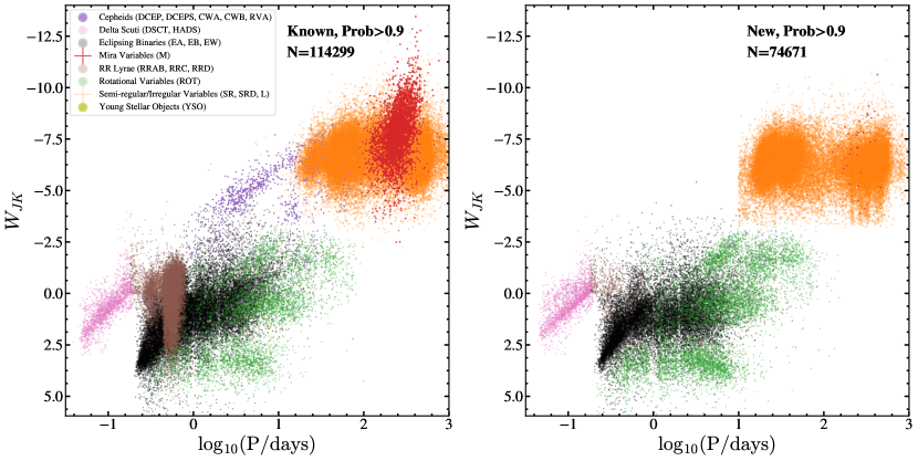
The combined Wesenheit $W_{JK}$ period-luminosity relationship (PLR) diagram for the periodic variables with $\rm Prob>0.9$ is shown in Figure 7. The PLR sequences for the Cepheids are well defined (Soszynski et al., 2005). Sharp PLR sequences can also be seen for Delta Scuti variables and contact binaries. The Mira variables also form a distinct PLR sequence beyond $P>100$ d. The slight deficits of variables at the aliases of a sidereal day (e.g., $P\approx 1$ d, $P\approx 2$ d, $P\approx 30$ d, etc.) are due to the quality checks implemented in $\S 3.5$.

Figure 7: The Wesenheit $W_{JK}$ PLR diagram for the periodic variables with $\rm Prob>0.9$, that have already been discovered (left), and the new discoveries (right).

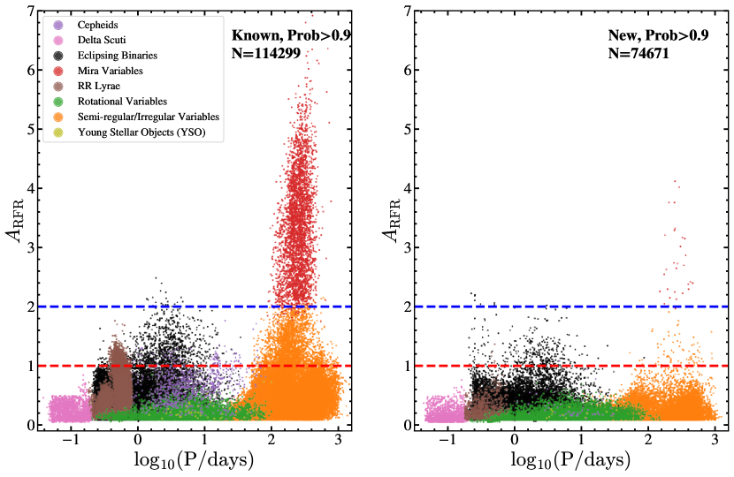
The period-amplitude plot for the periodic variables with $\rm Prob>0.9$ is shown in Figure 8. The high prior completeness of the Mira, RR Lyrae and Cepheid variables is evident. We do not discover many of these variables in this work. The large majority (${\sim}98.7\%$) of the new discoveries are of different variable types with smaller variability amplitudes and/or weak periodicity.

Figure 8: Period-amplitude plot for the for the periodic variables with $\rm Prob>0.9$, that have already been discovered (left), and the new discoveries (right). Reference amplitudes of 1 and 2 mag are shown in red and blue respectively.

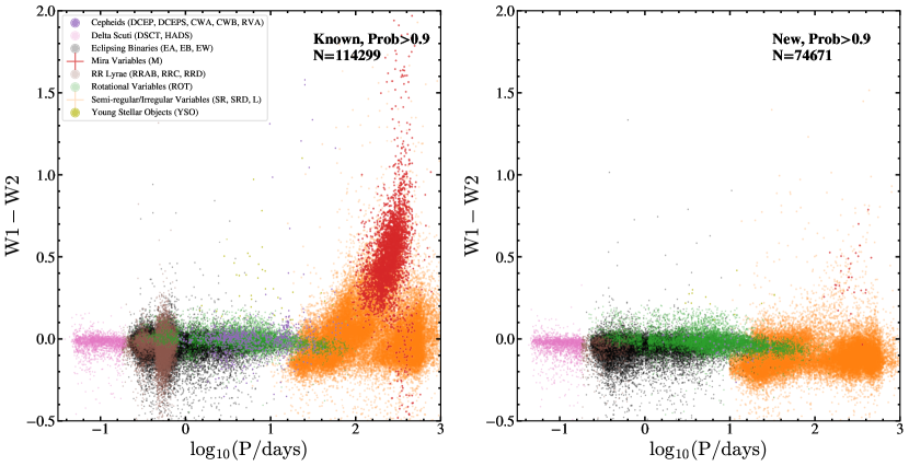
We also examine the period-color relationship of the variables in the AllWISE (Cutri et al., 2013; Wright et al., 2010) $\rm W_{1}-\rm W_{2}$ color space in Figure 9. Most variables have $\rm W_{1}-\rm W_{2}$ $\sim 0$, but the NIR infrared-excess increases with increasing period for the long period variables. This is even more dramatic for the Mira variables. Dust formation is commonly traced through infrared excesses. Our findings agree with McDonald et al. (2018), for example, that strong mass loss and increased dust formation first occurs for pulsation periods of $P{\gtrsim}60$ d for Galactic stars.

Figure 9: The period vs. $\rm W_{1}-\rm W_{2}$ color diagram for the variables with $\rm Prob>0.9$, that have already been discovered (left), and the new discoveries (right).

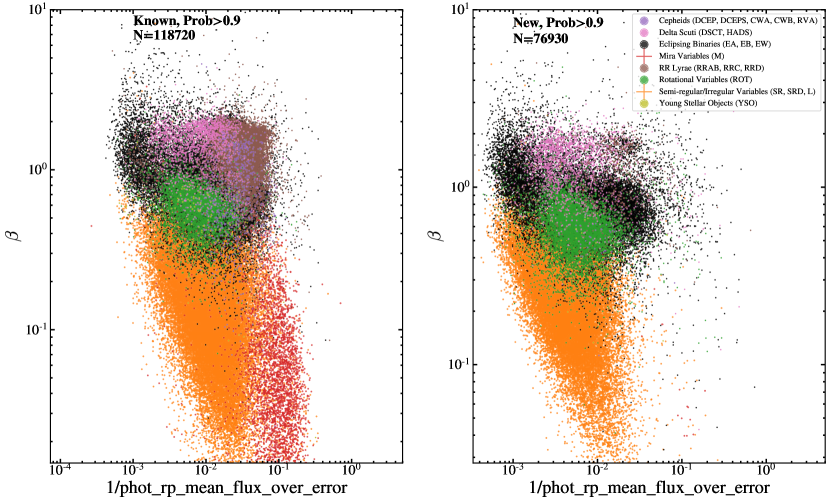
As an external check of our classifications, we used data from our cross-match to Gaia DR2 (Gaia Collaboration et al., 2018a) to produce Figure 10. We define a “variability” color $\beta$,

$$\beta=\rm phot\_bp\_mean\_flux\_error/phot\_rp\_mean\_flux\_error\,,$$ (8)

which is a measure of the difference in variability between the bluer and redder Gaia bands and compare it to the inverse of the quantity phot_rp_mean_flux_over_error which is a measure of the mean signal to noise ratio. The different groups of variables fall in distinct regions, with red pulsating variables having smaller values of $\beta$ compared to bluer variables. Comparing the known variables and the new discoveries, we find that the new discoveries mostly fall in the same regions as the known variables. This provides an independent confirmation of the purity of the newly discovered variables and validates our quality assurance methodology in $\S 3.5$.

Figure 10: The Gaia DR2 BP/RP variability ratio $\beta$ against 1/$\rm phot\_rp\_mean\_flux\_over\_error$

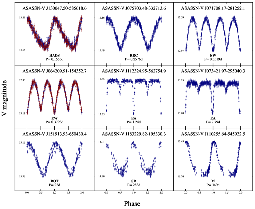
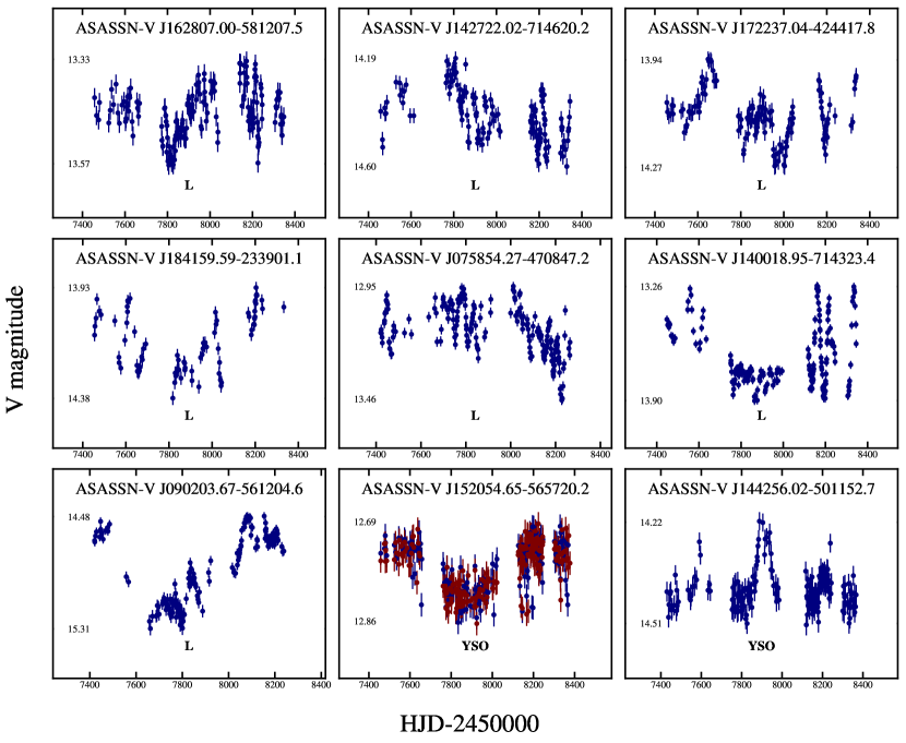
Examples of the newly identified periodic variables are shown in Figure 11 and examples of the newly discovered irregular variables are shown in Figure 12. The light curves for the red giant pulsators, including the irregular variables, are complex, and often multi-periodic, which requires further Fourier analysis. In order to better understand these pulsating red giants, Percy, & Fenaux (2019) recommended a more detailed analysis, combining visual inspection of the light curves and a more advanced period analysis, in lieu of the automated classification used by ASAS-SN.

Figure 11: Phased light curves for examples of the newly discovered periodic variables. The light curves are scaled by their minimum and maximum V-band magnitudes. Different colored points correspond to data from the different ASAS-SN cameras. The different variability types are defined in Table 5.

Figure 12: Light curves for examples of the newly discovered irregular variables. The format is the same as for Fig. 11

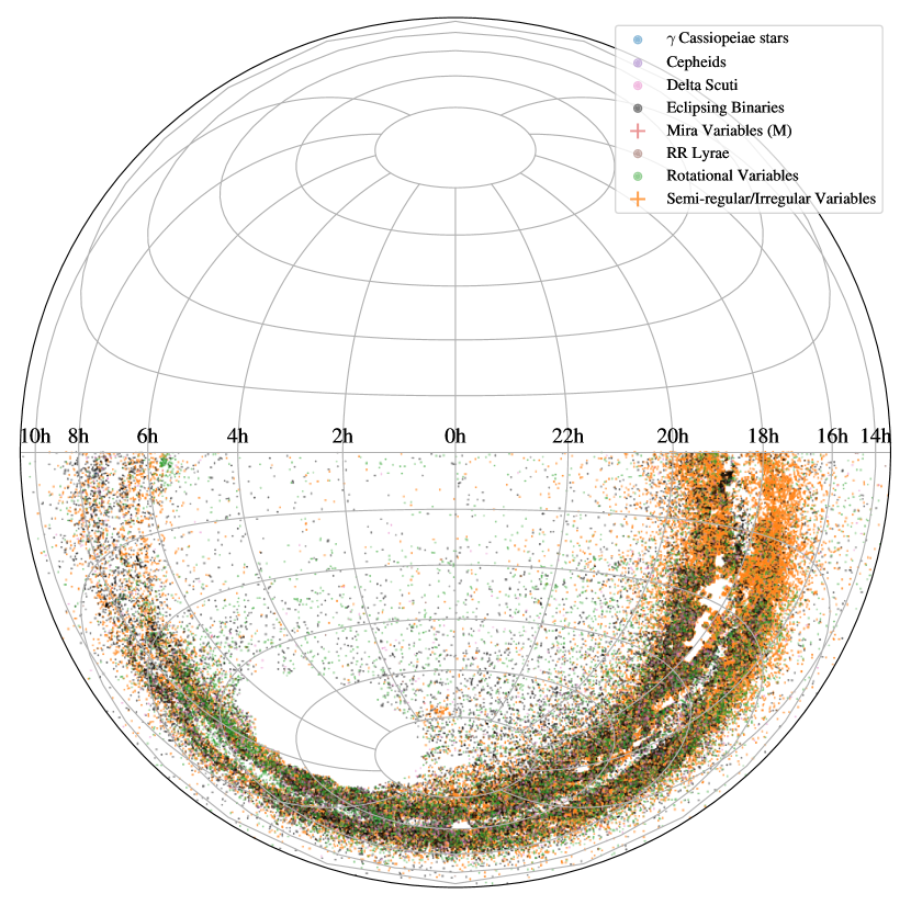
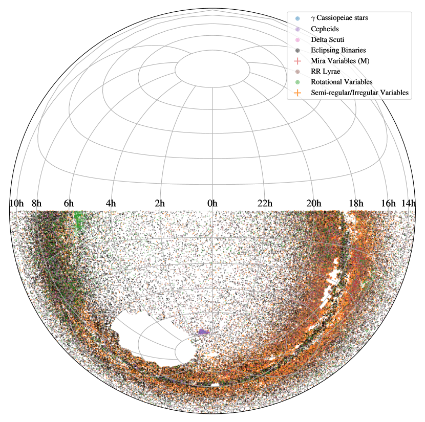
We illustrate the sky distribution of the newly discovered variables in Figure 13. Most of these discoveries are clustered towards the Galactic disk, as is expected. We note the scarcity of high amplitude Mira variables, RR Lyrae and Cepheid variables and the abundance of lower amplitude semi-regular/irregular variables among the newly discovered variables. Variables with large amplitudes and strong periodicity are relatively easily discovered and characterized by wide field photometric surveys, so the existing completeness of these variable types is very high. The gaps in coverage will be rectified in the next paper in this series. We also show the sky distribution of the known variables identified in this work in Figure 14. Here, we note the abundance of Mira variables, eclipsing binaries and Cepheid variables that have been discovered by previous surveys.

Figure 13: Spatial distribution of the $\sim 88,300$ newly discovered variables in Equatorial coordinates. Sources in the gap centered at the Southern Ecliptic Pole ($\alpha=6$ h, $\delta=-66.55$ deg) were analyzed in Jayasinghe et al. (2019b). The other gaps are in the APASS catalog.

Figure 14: Spatial distribution of the $\sim 131,900$ known variables in Equatorial coordinates. Sources in the gap centered at the Southern Ecliptic Pole ($\alpha=6$ h, $\delta=-66.55$ deg) were analyzed in Jayasinghe et al. (2019b). The other gaps are in the APASS catalog.

5 Conclusions

We systematically searched for variable sources with $V<17$ mag in the southern hemisphere ($\delta<0$ deg), excluding the ${\sim}1.3$M sources near the Southern Ecliptic Pole which were analyzed in Paper III. Through our search, we identified ${\sim}220,000$ variable sources, of which ${\sim}88,300$ are new discoveries. The sample of new variables includes ${\sim}48,000$ red pulsating variables, ${\sim}23,000$ eclipsing binaries, ${\sim}2,200$ $\delta$-Scuti variables and ${\sim}10,200$ rotational variables.

The V-band light curves of all the ${\sim}30.1$M sources studied in this work are available online at the ASAS-SN Photometry Database (https://asas-sn.osu.edu/photometry). We have also updated the ASAS-SN variable stars database (https://asas-sn.osu.edu/variables) with the light curves of these new variables. Most of these sources will also fall into the TESS footprint, thus short baseline TESS light curves that possess better photometric precision can also be obtained to complement the long baseline ASAS-SN light curves.

This work greatly improves the completeness of bright variables in the Southern hemisphere and provides long baseline V-band light curves. In particular, we have significantly improved the completeness of lower amplitude variables. As part of our ongoing effort to systematically analyze all the ${\sim}50$ million $V<17$ mag APASS sources for variability, we will next update this database with the light curves for the sources across the northern hemisphere and include the light curves for sources missing from the APASS DR9 catalog.

References

- Alard (2000) Alard, C. 2000, A&AS, 144, 363
- Alard & Lupton (1998) Alard, C., & Lupton, R. H. 1998, ApJ, 503, 325
- Alcock et al. (1997) Alcock, C., Allsman, R. A., Alves, D., et al. 1997, ApJ, 486, 697
- Astropy Collaboration et al. (2013) Astropy Collaboration, Robitaille, T. P., Tollerud, E. J., et al. 2013, A&A, 558, A33
- Bailer-Jones et al. (2018) Bailer-Jones, C. A. L., Rybizki, J., Fouesneau, M., Mantelet, G., & Andrae, R. 2018, AJ, 156, 58
- Beaton et al. (2018) Beaton, R. L., Bono, G., Braga, V. F., et al. 2018, Space Sci. Rev., 214, 113
- Bhatti et al. (2018) Bhatti, W., Bouma, L. G., Wallace, J., et al. 2018, astrobase, v0.3.8, Zenodo, http://doi.org/10.5281/zenodo.1185231
- Breger (1979) Breger, M. 1979, PASP, 91, 5
- Breiman (2001) Breiman, L. 2001, Machine Learning, 45, 1
- Brown et al. (2013) Brown, T. M., Baliber, N., Bianco, F. B., et al. 2013, PASP, 125, 1031
- Chen et al. (2018) Chen, X., Wang, S., Deng, L., et al. 2018, ApJS, 237, 28
- Clarke (2002) Clarke, D. 2002, A&A, 386, 763
- Cutri et al. (2013) Cutri, R. M., & et al. 2013, VizieR Online Data Catalog, 2328,
- Derue et al. (2002) Derue, F., Marquette, J.-B., Lupone, S., et al. 2002, A&A, 389, 149
- Drake et al. (2014) Drake, A. J., Graham, M. J., Djorgovski, S. G., et al. 2014, ApJS, 213, 9
- Feast, & Whitelock (2014) Feast, M., & Whitelock, P. A. 2014, Setting the Scene for Gaia and LAMOST, 40.
- Fernández-Trincado et al. (2015) Fernández-Trincado, J. G., Vivas, A. K., Mateu, C. E., et al. 2015, Astronomy and Astrophysics, 574, A15
- Gaia Collaboration et al. (2018a) Gaia Collaboration, Brown, A. G. A., Vallenari, A., et al. 2018, arXiv:1804.09365
- Gaia Collaboration et al. (2018b) Gaia Collaboration, Eyer, L., Rimoldini, L., et al. 2018, arXiv:1804.09382
- Gaia Collaboration et al. (2018c) Gaia Collaboration, Helmi, A., van Leeuwen, F., et al. 2018, A&A, 616, A12.
- Graczyk et al. (2014) Graczyk, D., Pietrzyński, G., Thompson, I. B., et al. 2014, ApJ, 780, 59
- Heinze et al. (2018) Heinze, A. N., Tonry, J. L., Denneau, L., et al. 2018, arXiv:1804.02132
- Henden et al. (2015) Henden, A. A., Levine, S., Terrell, D., & Welch, D. L. 2015, American Astronomical Society Meeting Abstracts #225, 225, 336.16
- Holl et al. (2018) Holl, B., Audard, M., Nienartowicz, K., et al. 2018, arXiv:1804.09373
- Holtzman et al. (2015) Holtzman, J. A., Shetrone, M., Johnson, J. A., et al. 2015, AJ, 150, 148
- Holoien et al. (2014) Holoien, T. W.-S., Prieto, J. L., Bersier, D., et al. 2014, MNRAS, 445, 3263
- Holoien et al. (2016) Holoien, T. W.-S., Kochanek, C. S., Prieto, J. L., et al. 2016, MNRAS, 455, 2918
- Holoien et al. (2017) Holoien, T. W.-S., Brown, J. S., Stanek, K. Z., et al. 2017, MNRAS, 471, 4966
- Holoien et al. (2018a) Holoien, T. W.-S., Brown, J. S., Vallely, P. J., et al. 2018, arXiv:1811.08904
- Holoien et al. (2018b) Holoien, T. W.-S., Huber, M. E., Shappee, B. J., et al. 2018, arXiv:1808.02890
- Jayasinghe et al. (2018a) Jayasinghe, T., Kochanek, C. S., Stanek, K. Z., et al. 2018, MNRAS, 477, 3145
- Jayasinghe et al. (2018b) Jayasinghe, T., Stanek, K. Z., Kochanek, C. S., et al. 2018, Research Notes of the American Astronomical Society, 2, 181
- Jayasinghe et al. (2018c) Jayasinghe, T., Stanek, K. Z., Kochanek, C. S., et al. 2018, Research Notes of the American Astronomical Society, 2, 125
- Jayasinghe et al. (2018d) Jayasinghe, T., Stanek, K. Z., Kochanek, C. S., et al. 2018, arXiv e-prints, arXiv:1901.00005
- Jayasinghe et al. (2019a) Jayasinghe, T., Stanek, K. Z., Kochanek, C. S., et al. 2019, MNRAS, 486, 1907
- Jayasinghe et al. (2019b) Jayasinghe T., et al., 2019, MNRAS, 485, 961
- Jayasinghe et al. (2019c) Jayasinghe, T., Stanek, K. Z., Kochanek, C. S., et al. 2019, The Astronomer’s Telegram, 12836, 1
- Kim & Bailer-Jones (2016) Kim, D.-W., & Bailer-Jones, C. A. L. 2016, A&A, 587, A18
- Kinemuchi et al. (2006) Kinemuchi, K., Smith, H. A., Woźniak, P. R., McKay, T. A., & ROTSE Collaboration 2006, AJ, 132, 1202
- Kochanek et al. (2017) Kochanek, C. S., Shappee, B. J., Stanek, K. Z., et al. 2017, PASP, 129, 104502
- Kovács et al. (2002) Kovács, G., Zucker, S., & Mazeh, T. 2002, A&A, 391, 369
- Lafler & Kinman (1965) Lafler, J., & Kinman, T. D. 1965, ApJS, 11, 216
- Lebzelter et al. (2018) Lebzelter, T., Mowlavi, N., Marigo, P., et al. 2018, arXiv:1808.03659
- Leavitt (1908) Leavitt, H. S. 1908, Annals of Harvard College Observatory, 60, 87
- Liao et al. (2019) Liao, S.-L., Qi, Z.-X., Guo, S.-F., & Cao, Z.-H. 2019, Research in Astronomy and Astrophysics, 19, 029
- Lopez de Coca et al. (1990) Lopez de Coca, P., Rolland, A., Rodriguez, E., & Garrido, R. 1990, A&AS, 83, 51
- McDonald et al. (2018) McDonald, I., De Beck, E., Zijlstra, A. A., & Lagadec, E. 2018, MNRAS, 481, 4984
- Madore (1982) Madore, B. F. 1982, ApJ, 253, 575
- Marrese et al. (2019) Marrese, P. M., Marinoni, S., Fabrizio, M., et al. 2019, A&A, 621, A144
- Mateu et al. (2012) Mateu, C., Vivas, A. K., Downes, J. J., et al. 2012, Monthly Notices of the Royal Astronomical Society, 427, 3374
- Mateu, & Vivas (2018) Mateu, C., & Vivas, A. K. 2018, Monthly Notices of the Royal Astronomical Society, 479, 211
- Matsunaga (2018) Matsunaga, N. 2018, Rediscovering Our Galaxy, 57.
- Matsunaga et al. (2006) Matsunaga, N., Fukushi, H., Nakada, Y., et al. 2006, MNRAS, 370, 1979
- Ochsenbein et al. (2000) Ochsenbein, F., Bauer, P., & Marcout, J. 2000, A&AS, 143, 23
- Oelkers et al. (2018) Oelkers, R. J., Rodriguez, J. E., Stassun, K. G., et al. 2018, AJ, 155, 39
- Pawlak et al. (2016) Pawlak, M., Soszyński, I., Udalski, A., et al. 2016, Acta Astron., 66, 421
- Pawlak et al. (2019) Pawlak, M., Pejcha, O., Jakubčík, P., et al. 2019, MNRAS, 1644
- Pedregosa et al. (2012) Pedregosa, F., Varoquaux, G., Gramfort, A., et al. 2012, arXiv:1201.0490
- Percy, & Fenaux (2019) Percy, J. R., & Fenaux, L. 2019, arXiv e-prints, arXiv:1905.03279
- Pietrzyński et al. (2013) Pietrzyński, G., Graczyk, D., Gieren, W., et al. 2013, Nature, 495, 76
- Pojmanski (2002) Pojmanski, G. 2002, Acta Astron., 52, 397
- Ricker et al. (2015) Ricker, G. R., Winn, J. N., Vanderspek, R., et al. 2015, Journal of Astronomical Telescopes, Instruments, and Systems, 1, 014003
- Rodríguez et al. (2018) Rodríguez, R., Schmidt, S. J., Jayasinghe, T., et al. 2018, Research Notes of the American Astronomical Society, 2, 8
- Scargle (1982) Scargle, J. D. 1982, ApJ, 263, 835
- Schwarzenberg-Czerny (1996) Schwarzenberg-Czerny, A. 1996, ApJ, 460, L107
- Shappee et al. (2014) Shappee, B. J., Prieto, J. L., Grupe, D., et al. 2014, ApJ, 788, 48
- Shields et al. (2018) Shields, J. V., Jayasinghe, T., Stanek, K. Z., et al. 2018, arXiv:1809.04075
- Skrutskie et al. (2006) Skrutskie, M. F., Cutri, R. M., Stiening, R., et al. 2006, AJ, 131, 1163
- Soszynski et al. (2005) Soszynski, I., Udalski, A., Kubiak, M., et al. 2005, Acta Astron., 55, 331.
- Soszyński et al. (2016) Soszyński, I., Pawlak, M., Pietrukowicz, P., et al. 2016, Acta Astron., 66, 405
- Stassun et al. (2018) Stassun, K. G., Oelkers, R. J., Pepper, J., et al. 2018, AJ, 156, 102
- Stetson (1996) Stetson, P. B. 1996, PASP, 108, 851
- Taylor (2005) Taylor, M. B. 2005, Astronomical Data Analysis Software and Systems XIV, 347, 29
- Thompson et al. (2018) Thompson, T. A., Kochanek, C. S., Stanek, K. Z., et al. 2018, arXiv:1806.02751
- Tonry et al. (2018a) Tonry, J. L., Denneau, L., Heinze, A. N., et al. 2018, PASP, 130, 064505
- Tonry et al. (2018b) Tonry, J. L., Denneau, L., Flewelling, H., et al. 2018, ApJ, 867, 105
- Torres et al. (2010) Torres, G., Andersen, J., & Giménez, A. 2010, A&ARv, 18, 67
- Tucker et al. (2018) Tucker, M. A., Shappee, B. J., Holoien, T. W.-S., et al. 2018, arXiv:1808.07875
- Udalski (2003) Udalski, A. 2003, Acta Astron., 53, 291
- Udalski et al. (2018) Udalski, A., Soszyński, I., Pietrukowicz, P., et al. 2018, Acta Astronomica, 68, 315
- VanderPlas (2018) VanderPlas, J. T. 2018, ApJS, 236, 16
- Von Neumann et al. (1941) Von Neumann, J., Kent, R., Bellinson, H., & Hart, B. T. 1941,The Annals of Mathematical Statistics, 12, 153
- Watson et al. (2006) Watson, C. L., Henden, A. A., & Price, A. 2006, Society for Astronomical Sciences Annual Symposium, 25, 47
- Whitelock et al. (2008) Whitelock, P. A., Feast, M. W., & Van Leeuwen, F. 2008, Monthly Notices of the Royal Astronomical Society, 386, 313
- Wright et al. (2010) Wright, E. L., Eisenhardt, P. R. M., Mainzer, A. K., et al. 2010, AJ, 140, 1868
- Woźniak et al. (2004) Woźniak, P. R., Vestrand, W. T., Akerlof, C. W., et al. 2004, AJ, 127, 2436
- Zechmeister & Kürster (2009) Zechmeister, M., & Kürster, M. 2009, A&A, 496, 577