Who is Afraid of Big Bad Minima?
Analysis of Gradient-Flow in a Spiked Matrix-Tensor Model

Stefano Sarao Mannelli Institut de physique théorique, Université Paris Saclay, CNRS, CEA, 91191 Gif-sur-Yvette, France Giulio Biroli Laboratoire de Physique de l’Ecole normale supérieure ENS, Université PSL, CNRS, Sorbonne Université, Université Paris-Diderot, Sorbonne Paris Cité Paris, France Chiara Cammarota Department of Mathematics, King’s College London, Strand London WC2R 2LS, UK Florent Krzakala Laboratoire de Physique de l’Ecole normale supérieure ENS, Université PSL, CNRS, Sorbonne Université, Université Paris-Diderot, Sorbonne Paris Cité Paris, France Lenka Zdeborová Institut de physique théorique, Université Paris Saclay, CNRS, CEA, 91191 Gif-sur-Yvette, France
Abstract

Gradient-based algorithms are effective for many machine learning tasks, but despite ample recent effort and some progress, it often remains unclear why they work in practice in optimising high-dimensional non-convex functions and why they find good minima instead of being trapped in spurious ones. Here we present a quantitative theory explaining this behaviour in a spiked matrix-tensor model. Our framework is based on the Kac-Rice analysis of stationary points and a closed-form analysis of gradient-flow originating from statistical physics. We show that there is a well defined region of parameters where the gradient-flow algorithm finds a good global minimum despite the presence of exponentially many spurious local minima. We show that this is achieved by surfing on saddles that have strong negative direction towards the global minima, a phenomenon that is connected to a BBP-type threshold in the Hessian describing the critical points of the landscapes.

1 Introduction

A common theme in machine learning and optimisation is to understand the behaviour of gradient descent methods for non-convex problems with many minima. Despite the non-convexity, such methods often successfully optimise models such as neural networks, matrix completion and tensor factorisation. This has motivated a recent spur in research attempting to characterise the properties of the loss landscape that may shed some light on the reason of such success. Without the aim of being exhaustive these include [1, 2, 3, 4, 5, 6, 7, 8, 9, 10, 11].

Over the last few years, a popular line of research has shown, for a variety of systems, that spurious local minima are not present in certain regimes of parameters. When the signal-to-noise ratio is large enough, the success of gradient descent can thus be understood by a trivialisation transition in the loss landscape: either there is only a single minima, or all minima become "good", and no spurious minima can trap the dynamics. This is what happens, for instance, in the limit of small noise and abundance of data for matrix completion and tensor factorization [3, 8], or for some very large neural networks [1, 2]. However, it is often observed in practice that these guarantees fall short of explaining the success of gradient descent, that is empirically observed to find good minima very far from the regime under mathematical control. In fact, gradient-descent-based algorithms may be able to perform well even when spurious local minima are present because the basins of attraction of the spurious minima may be small and the dynamics might be able to avoid them. Understanding this behaviour requires, however, a very detailed characterisation of the dynamics and of the landscape, a feat which is not yet possible in full generality.

A fruitful direction is the study of Gaussian functions on the N𝑁N-dimensional sphere, known as p𝑝p-spin spherical spin glass models in the physics literature, and as isotropic models in the Gaussian process literature [12, 13, 14, 15, 16]. In statistics and machine learning, these models have appeared following the studies of spiked matrix and tensor models [17, 18, 19]. In particular, a very recent work [20] showed explicitly that for a spiked matrix-tensor model the gradient-flow algorithm indeed reaches global minimum even when spurious local minima are present and the authors estimated numerically the corresponding regions of parameters. In this work we consider this very same model and explain the mechanism by which the spurious local minima are avoided, and develop a quantitative theoretical framework that we believe has a strong potential to be generic and extendable to a much broader range of models in high-dimensional inference and neural networks.

The Spiked Matrix-Tensor Model. The spiked matrix-tensor model has been recently proposed to be a prototypical model for non-convex high-dimensional optimisation where several non-trivial regimes of cost-landscapes can be displayed quantitatively by tuning the parameters [21, 20]. In this model, one aims at reconstructing a hidden vector (i.e. the spike) 𝝈superscript𝝈\boldsymbol{\sigma}^{*} from the observation of a noisy version of both the rank-one matrix and rank-one tensor created from the spike. Using the following notation: bold lowercase symbols represent vectors, bold uppercase symbols represent matrices or tensors, and ,\langle\cdot,\cdot\rangle represent the scalar product, the model is defined as follows: given a signal (or spike), 𝝈superscript𝝈\boldsymbol{\sigma}^{*}, uniformly sampled on the N𝑁N-dimensional hyper-sphere of radius 111, it is given a tensor 𝑻𝑻\boldsymbol{T} and a matrix 𝒀𝒀\boldsymbol{Y} such that

Ti1ip=ηi1ip+N(p1)!σi1σip,subscript𝑇subscript𝑖1subscript𝑖𝑝subscript𝜂subscript𝑖1subscript𝑖𝑝𝑁𝑝1subscriptsuperscript𝜎subscript𝑖1subscriptsuperscript𝜎subscript𝑖𝑝\displaystyle T_{i_{1}\dots i_{p}}=\eta_{i_{1}\dots i_{p}}+\sqrt{N(p-1)!}\,\sigma^{*}_{i_{1}}\dots\sigma^{*}_{i_{p}}\,, (1)
Yij=ηij+Nσiσj,subscript𝑌𝑖𝑗subscript𝜂𝑖𝑗𝑁subscriptsuperscript𝜎𝑖subscriptsuperscript𝜎𝑗\displaystyle Y_{ij}=\eta_{ij}+\sqrt{N}\sigma^{*}_{i}\sigma^{*}_{j}\,, (2)

where ηi1ipsubscript𝜂subscript𝑖1subscript𝑖𝑝\eta_{i_{1}\dots i_{p}} and ηijsubscript𝜂𝑖𝑗\eta_{ij} are Gaussian random variables of variance ΔpsubscriptΔ𝑝\Delta_{p} and Δ2subscriptΔ2\Delta_{2} respectively. Neglecting constant terms, the maximum likelihood estimation of the ground truth, 𝝈superscript𝝈\boldsymbol{\sigma}^{*}, corresponds to minimization of the following loss function:

(𝝈|𝑻,𝒀)=(p1)!ΔpNi1<<ipTi1ipσi1σip1Δ2Ni<jYijσiσj=conditional𝝈𝑻𝒀𝑝1subscriptΔ𝑝𝑁subscriptsubscript𝑖1subscript𝑖𝑝subscript𝑇subscript𝑖1subscript𝑖𝑝subscript𝜎subscript𝑖1subscript𝜎subscript𝑖𝑝1subscriptΔ2𝑁subscript𝑖𝑗subscript𝑌𝑖𝑗subscript𝜎𝑖subscript𝜎𝑗absent\text{\large$\ell$}(\boldsymbol{\sigma}|\boldsymbol{T},\boldsymbol{Y})=-\frac{\sqrt{(p-1)!}}{\Delta_{p}\sqrt{N}}\sum_{i_{1}<\dots<i_{p}}T_{i_{1}\dots i_{p}}\sigma_{i_{1}}\dots\sigma_{i_{p}}-\frac{1}{\Delta_{2}\sqrt{N}}\sum_{i<j}Y_{ij}\sigma_{i}\sigma_{j}= (3)
(p1)!ΔpNi1<<ipηi1ipσi1σip1Δ2Ni<jηijσiσj𝝈,𝝈ppΔp𝝈,𝝈22Δ2.𝑝1subscriptΔ𝑝𝑁subscriptsubscript𝑖1subscript𝑖𝑝subscript𝜂subscript𝑖1subscript𝑖𝑝subscript𝜎subscript𝑖1subscript𝜎subscript𝑖𝑝1subscriptΔ2𝑁subscript𝑖𝑗subscript𝜂𝑖𝑗subscript𝜎𝑖subscript𝜎𝑗superscript𝝈superscript𝝈𝑝𝑝subscriptΔ𝑝superscript𝝈superscript𝝈22subscriptΔ2-\frac{\sqrt{(p-1)!}}{\Delta_{p}\sqrt{N}}\sum_{i_{1}<\dots<i_{p}}\eta_{i_{1}\dots i_{p}}\sigma_{i_{1}}\dots\sigma_{i_{p}}-\frac{1}{\Delta_{2}\sqrt{N}}\sum_{i<j}\eta_{ij}\sigma_{i}\sigma_{j}-\frac{\langle\boldsymbol{\sigma},\boldsymbol{\sigma}^{*}\rangle^{p}}{p\Delta_{p}}-\frac{\langle\boldsymbol{\sigma},\boldsymbol{\sigma}^{*}\rangle^{2}}{2\Delta_{2}}\,.

The first two contributions of the last equation will be denoted ϵpsubscriptitalic-ϵ𝑝\epsilon_{p} and ϵ2subscriptitalic-ϵ2\epsilon_{2} in the following. While the matricial observations correspond to a quadratic term and thus to a simple loss-landscape, the additional order-p𝑝p tensor contributes towards a rough non-convex loss landscape. As ΔpsubscriptΔ𝑝\Delta_{p}\!\rightarrow\!\infty the information Ti1ipsubscript𝑇subscript𝑖1subscript𝑖𝑝T_{i_{1}\dots i_{p}} becomes irrelevant and the landscape becomes trivial, while in the opposite limit Δ2subscriptΔ2\Delta_{2}\!\rightarrow\!\infty, the landscape becomes extremely rough and complex as analyzed recently in [16, 22].

We shall consider the behaviour of the gradient-flow (GF) algorithm aiming to minimise the loss:

σ˙i(t)=μ(t)σi(t)(𝝈(t)|𝑻,𝒀)σi(t),subscript˙𝜎𝑖𝑡𝜇𝑡subscript𝜎𝑖𝑡conditional𝝈𝑡𝑻𝒀subscript𝜎𝑖𝑡\dot{\sigma}_{i}(t)=-\mu(t)\sigma_{i}(t)-\frac{\partial\text{\large$\ell$}(\boldsymbol{\sigma}(t)|\boldsymbol{T},\boldsymbol{Y})}{\partial\sigma_{i}(t)}\,, (4)

where μ(t)𝜇𝑡\mu(t) enforces that 𝝈(t)𝝈𝑡\boldsymbol{\sigma}(t) belongs to the hyper-sphere of radius N𝑁N and will be referred to as the spherical constraint. The algorithm is initialised in a random point drawn uniformly on the hyper-sphere, thus initially having no correlation with the ground-truth signal. We view the gradient-flow as a prototype of gradient-descent-based algorithms that are the work-horse of current machine learning.
Refer to caption
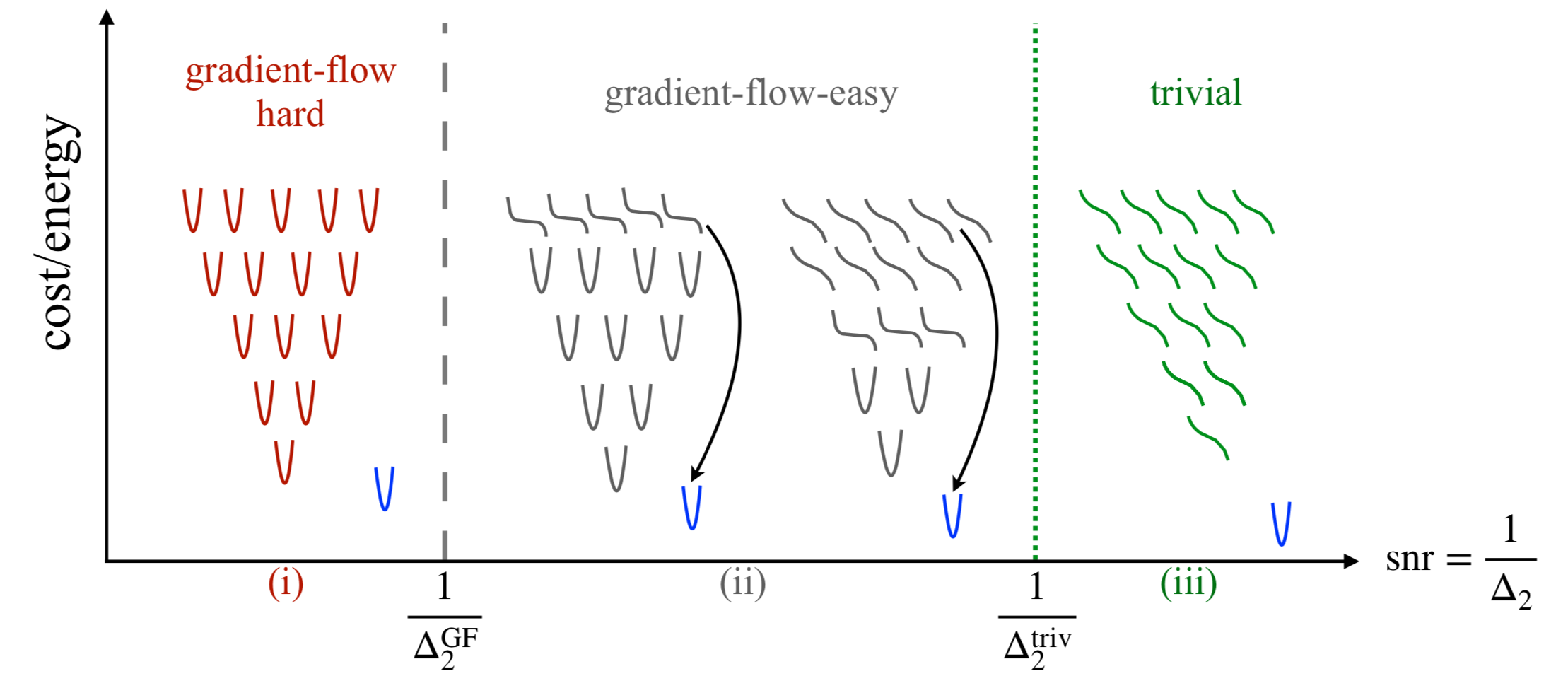
Figure 1: Cartoon illustrating the mechanism by which gradient-flow avoids spurious local minima in the spiked matrix-tensor model. As the signal-to-noise (snrsnr\rm snr) ratio 1/Δ21subscriptΔ21/\Delta_{2} is increased, the spurious local minima that attract the randomly initialised GF algorithm develop a single negative direction towards the global minimum before the others, in particular the lower-cost spurious local minima, do. This has drastic consequences on the GF algorithm. In region (i), for snr<1/Δ2GFsnr1superscriptsubscriptΔ2GF{\rm snr}<1/\Delta_{2}^{\rm GF}, the algorithm goes down the landscape, eventually reaches the high-energy threshold minima and remains stuck. In region (ii), however, these threshold minima are turned into saddles with a strong negative direction towards the signal. The algorithm is initially reaching these minima-turned-saddles, surfing on the negative slope, it then turns towards the "good" minima correlated with the signal, avoiding the exponentially many spurious minima at lower energies. The main technical contribution of this paper is a quantitative description of this scenario, including a simple formula for the corresponding threshold Δ2GFsuperscriptsubscriptΔ2GF\Delta_{2}^{\rm GF}, eq. (5). As the snr is further increased, the negative direction appears in lower and lower minima until the trivialization transition in region (iii): for snr>1/Δ2trivsnr1superscriptsubscriptΔ2triv{\rm snr}>1/\Delta_{2}^{\rm triv}, all the spurious minima have been turned into saddles.

Main Contributions. The first main result of this paper is the expression for the threshold below which the gradient-flow algorithm finds a configuration correlated the hidden spike. This threshold is established in the asymptotic limit of large N𝑁N, fixed p𝑝p and ΔpsubscriptΔ𝑝\Delta_{p}, and reads:

Δ2GF(Δp,p)Δp+Δp2+4(p1)Δp2(p1).subscriptsuperscriptΔGF2subscriptΔ𝑝𝑝subscriptΔ𝑝superscriptsubscriptΔ𝑝24𝑝1subscriptΔ𝑝2𝑝1\Delta^{\rm GF}_{2}(\Delta_{p},p)\equiv\frac{-\Delta_{p}+\sqrt{\Delta_{p}^{2}+4(p-1)\Delta_{p}}}{2(p-1)}\,. (5)

We find that (i) for Δ2<Δ2GFsubscriptΔ2subscriptsuperscriptΔGF2\Delta_{2}<\Delta^{\rm GF}_{2} the gradient flow reaches in finite time the global minimum, well correlated with the signal, while (ii) for Δ2>Δ2GFsubscriptΔ2subscriptsuperscriptΔGF2\Delta_{2}>\Delta^{\rm GF}_{2} the algorithm remains uncorrelated with the signal for all times that do not grow as N𝑁N grows. We contrast it with the threshold Δ2triv<Δ2GFsuperscriptsubscriptΔ2trivsubscriptsuperscriptΔGF2\Delta_{2}^{\rm triv}<\Delta^{\rm GF}_{2}, established in [20], below which the energy landscape does not present any spurious local minima. Note that Δ2GFsubscriptsuperscriptΔGF2\Delta^{\rm GF}_{2} is less than Δ2AMP=1superscriptsubscriptΔ2AMP1\Delta_{2}^{\rm AMP}=1 [21], below which the best known algorithm, specifically the approximate message passing, works.

The second main result of this paper, is the insight we obtain on the behaviour of the gradient-flow in the loss landscape, that is summarised in Fig. 1. The key point is to consider the fate of the spurious local minima that attract the GF algorithm when the signal to noise ratio snr=1/Δ2snr1subscriptΔ2{\rm snr}=1/\Delta_{2} is increased. As the snrsnr{\rm snr} increases, these minima turn into saddles with a single negative direction towards the signal (a phenomenon that we analyze in the next section, and that turns out to be linked to the BBP transition [23] in random matrix theory), all that well before all the other spurious local minima disappear. We present two ways to quantify this insight:

(a) We use the Kac-Rice formula for the number of stationary points, as derived for the present model in [20]. In [20] this formula is used to quantify the region with no spurious local minima. Here we focus on a BBP-type of phase transition that is crucial in the derivation of this formula and deduce the GF threshold (5) from it.

(b) We use the CHSCK equations [24, 25] for closed-form description of the behaviour of the gradient-flow, as derived and numerically solved in [21, 20]. Building on dynamical theory of mean-field spin glasses we determine precisely when and how the algorithm escapes the manifold of zero overlap with the signal, leading again to the threshold (5).

Both these arguments are derived using reasoning common in theoretical physics. From a mathematically rigorous point of view the threshold (5) remains a conjecture and its rigorous proof is an interesting challenge for future work. We note that both the Kac-Rice approach [16] and the CHSCK equations [26] have been made rigorous in closely related problems. We believe that the reported results are not limited to the present model and we will investigate analytically and numerically other models and real-data-based learning in order to validate this theory and to understand its limitations.
Refer to caption
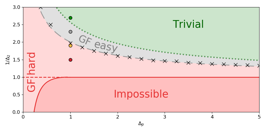
Figure 2: The phase diagram shows the different regions for gradient-flow behaviour, for the spiked matrix-tensor model with p=3𝑝3p=3. In the region shaded in red (light and dark), GF does not correlate with the signal, while it does in the grey and green regions. In the dark-red region obtaining correlation with the signal is impossible information-theoretically [21]. The possible region is divided by a red dashed line, below that line even best known algorithms are unable to obtain correlation with the signal [21]. The green region is characterised by a trivial landscape, i.e. all the spurious minima disappear [20]. The grey region is where gradient-flow succeeds to converge despite the presence of spurious minima. We marked with black crosses points predicting the gradient-flow threshold obtained numerically in [20], they perfectly agree with our theoretical prediction of the threshold (5), marked by the grey dashed line. The circles in colours are points that we will use to illustrate the different features of these regions.

2 Probing the Landscape by the Kac-Rice Method

The statistical properties of the landscape associated to the loss function (3) can be studied by the Kac-Rice method, which traces back to the statistical physics literature, see [27] for an overview, and was developed mathematically in [13, 14] and recently extended in [22].

The quantities of interest are the number of critical points at a given energy, 𝒩(ϵp,ϵ2)𝒩subscriptitalic-ϵ𝑝subscriptitalic-ϵ2{\mathcal{N}}(\epsilon_{p},\epsilon_{2}), and the Hessian matrix evaluated at those critical points. We analyse the logarithm of 𝒩(ϵp,ϵ2)𝒩subscriptitalic-ϵ𝑝subscriptitalic-ϵ2{\mathcal{N}}(\epsilon_{p},\epsilon_{2}), called the complexity. Since the complexity is a random quantity we compute its upper bound Σa(ϵp,ϵ2)=ln𝔼[𝒩(ϵp,ϵ2)]subscriptΣ𝑎subscriptitalic-ϵ𝑝subscriptitalic-ϵ2𝔼delimited-[]𝒩subscriptitalic-ϵ𝑝subscriptitalic-ϵ2\Sigma_{a}(\epsilon_{p},\epsilon_{2})=\ln\mathbb{E}[{\mathcal{N}}(\epsilon_{p},\epsilon_{2})], along the lines of [16, 20]. We have also computed its typical value Σq(ϵp,ϵ2)=𝔼[ln𝒩(ϵp,ϵ2)]subscriptΣ𝑞subscriptitalic-ϵ𝑝subscriptitalic-ϵ2𝔼delimited-[]𝒩subscriptitalic-ϵ𝑝subscriptitalic-ϵ2\Sigma_{q}(\epsilon_{p},\epsilon_{2})=\mathbb{E}[\ln{\mathcal{N}}(\epsilon_{p},\epsilon_{2})] along the lines of [22], i.e. non-rigorously using the replica symmetry assumption (see SM Sec. A). In what follows we focus on complexity of stationary points with no correlation with the signal, in which case analytical and numerical arguments (see SM Sec. A.2.1) indicate that Σa(ep,e2)subscriptΣ𝑎subscript𝑒𝑝subscript𝑒2\Sigma_{a}(e_{p},e_{2}) and Σq(ep,e2)subscriptΣ𝑞subscript𝑒𝑝subscript𝑒2\Sigma_{q}(e_{p},e_{2}) are either very close numerically or possibly equal. Thus, in the following, we will simply refer to the complexity Σ(ϵp,ϵ2)Σsubscriptitalic-ϵ𝑝subscriptitalic-ϵ2\Sigma(\epsilon_{p},\epsilon_{2}) without further specification.

In the Kac-Rice analysis the statistics of the Hessian, \mathcal{H}, of critical points plays a key role. It was shown in [20], and the argumentation is reproduced in the SM Sec. A.2, that \mathcal{H} has a simple form for the loss (3). It is a (N1)×(N1)𝑁1𝑁1(N-1)\times(N-1) matrix formed by the sum of three contributions: a random matrix 𝕎N1subscript𝕎𝑁1\mathbb{W}_{N-1} belonging to the Gaussian orthogonal ensemble (GOE), a matrix proportional to the identity, and a rank one projector in the direction of the signal. The expression of \mathcal{H} for critical points with null overlap m𝑚m with the signal and with energies ϵpsubscriptitalic-ϵ𝑝\epsilon_{p} and ϵ2subscriptitalic-ϵ2\epsilon_{2} reads:

=Q′′(1)[𝕎N1+t𝕀N1θ𝒆1𝒆1T]superscript𝑄′′1delimited-[]subscript𝕎𝑁1𝑡subscript𝕀𝑁1𝜃subscript𝒆1superscriptsubscript𝒆1𝑇\mathcal{H}=\sqrt{Q^{\prime\prime}(1)}\left[\mathbb{W}_{N-1}+t\,\mathbb{I}_{N-1}-\theta\,\boldsymbol{e}_{1}\boldsymbol{e}_{1}^{T}\right] (6)

with Q(x)=xppΔp+x22Δ2𝑄𝑥superscript𝑥𝑝𝑝subscriptΔ𝑝superscript𝑥22subscriptΔ2Q(x)=\frac{x^{p}}{p\Delta_{p}}+\frac{x^{2}}{2\Delta_{2}}, t=(pϵp+2ϵ2)/Q′′(1)𝑡𝑝subscriptitalic-ϵ𝑝2subscriptitalic-ϵ2superscript𝑄′′1t=-\left(p\epsilon_{p}+2\epsilon_{2}\right)/\sqrt{Q^{\prime\prime}(1)}, and θ=Q′′(0)/Q′′(1)𝜃superscript𝑄′′0superscript𝑄′′1\theta=Q^{\prime\prime}(0)\,/\sqrt{Q^{\prime\prime}(1)}. The normalisation of 𝕎N1subscript𝕎𝑁1\mathbb{W}_{N-1} is chosen such that Tr𝔼[𝕎N12]=1Tr𝔼delimited-[]superscriptsubscript𝕎𝑁121\mathrm{Tr}\mathbb{E}[\mathbb{W}_{N-1}^{2}]=1.

The Fate of the Spurious: The initial condition for the gradient-flow algorithm is a random configuration 𝝈0subscript𝝈0\boldsymbol{\sigma}_{0} uniformly drawn on the hyper-sphere. Such an initial condition clearly belongs to the large manifold of configurations uncorrelated with the ground-truth signal. We aim to investigate how does the gradient flow manage to escape from this initial manifold. For this purpose we focus on the properties of the landscape in the subspace where the overlap with the signal is zero, m=0𝑚0m=0.

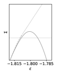
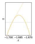
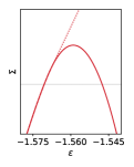
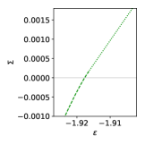
In Fig. 3, we plot the complexity at m=0𝑚0m=0 as a function of the energy ϵitalic-ϵ\epsilon

Σ(ϵ)=supϵp,ϵ2s.t. ϵp+ϵ2=ϵΣ(ϵp,ϵ2)|m=0Σitalic-ϵevaluated-atsubscriptsupremumsubscriptitalic-ϵ𝑝subscriptitalic-ϵ2s.t. subscriptitalic-ϵ𝑝subscriptitalic-ϵ2italic-ϵΣsubscriptitalic-ϵ𝑝subscriptitalic-ϵ2𝑚0\Sigma(\epsilon)=\sup_{\begin{subarray}{c}\epsilon_{p},\epsilon_{2}\\ \text{s.t. }\epsilon_{p}+\epsilon_{2}=\epsilon\end{subarray}}\Sigma(\epsilon_{p},\epsilon_{2})\Big{|}_{m=0}

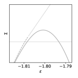
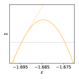
for the points 1/Δ2=1.9,2.3,2.71subscriptΔ21.92.32.71/\Delta_{2}=1.9,2.3,2.7 and Δp=1.0subscriptΔ𝑝1.0\Delta_{p}=1.0 (p=3𝑝3p=3), which are marked with circles of the corresponding colour in Fig. 2. We use discontinuous lines for the complexity of critical points that have at least one negative direction, and full lines for the complexity of local minima. A finding of [20], that holds for any value of ΔpsubscriptΔ𝑝\Delta_{p}, is that for small 1/Δ21subscriptΔ21/\Delta_{2} the majority of critical points with zero overlap with the signal at low enough energies are spurious minima; they disappear increasing 1/Δ21subscriptΔ21/\Delta_{2} above a ΔpsubscriptΔ𝑝\Delta_{p}-dependent value 1/Δ2triv1subscriptsuperscriptΔtriv21/\Delta^{\rm triv}_{2} corresponding to the green region of Fig. 2. In this part of the phase diagram, there are no spurious minima and the global minimum is correlated with the signal; this is an "easy" landscape for gradient flow which is therefore expected to succeed there. The main open question concerns the behavior for smaller values of 1/Δ21subscriptΔ21/\Delta_{2}: When does the existence of spurious minima, appearing in panel (b) and (c) of Fig. 3, start to be harmful to gradient flow?
Refer to caption
Refer to caption
Refer to caption
Figure 3: Complexity curves for the number of critical points for an overlap value m=0𝑚0m=0 at fixed Δp=1.0subscriptΔ𝑝1.0\Delta_{p}=1.0 for (from left to right) 1/Δ2=2.7,2.3,1.91subscriptΔ22.72.31.91/\Delta_{2}=2.7,2.3,1.9. The lines are dotted when the complexity is dominate by critical points having an extensive number of eigenvalues are negative, dashed when only one eigenvalue is negative, full when the points have only positive (or null) eigenvalues i.e. they are minima. The complexity of the minima is drawn in full lines with the same colours, and it merges with the complexity of stationary points when it becomes dominant.

In order to answer this question, we investigate more closely the nature of the spurious minima at different energies. We focus in particular on their Hessian, which plays a crucial role in order to understand which spurious minima have the largest basin of attraction and, hence, can trap the algorithm. For low signal-to-noise ratio, large ΔpsubscriptΔ𝑝\Delta_{p} and large Δ2subscriptΔ2\Delta_{2}, the spectrum of (6) is a shifted Wigner semicircle with support [Q′′(1)(2+t),Q′′(1)(2+t)]superscript𝑄′′12𝑡superscript𝑄′′12𝑡[\sqrt{Q^{\prime\prime}(1)}(-2+t),\sqrt{Q^{\prime\prime}(1)}(2+t)]. The effect of the projector (third contribution to the RHS of (6)) on the support of the spectrum is negligible as long as θ1𝜃1\theta\leq 1, as follows from the work on low-rank perturbations of random GOE matrices [23]. Moreover, the most numerous critical points at fixed energy ϵitalic-ϵ\epsilon are characterized by a t(ϵ)𝑡italic-ϵt(\epsilon) that is a monotonously decreasing function of ϵitalic-ϵ\epsilon, see Fig. 6 in the SM. Thus, moving towards higher energies, the spectrum of the Hessian shifts to the left, which indicates smaller curvature and wider minima. The transition between minima and saddles takes place at the threshold energy at which t(ϵth)=2𝑡subscriptitalic-ϵth2t(\epsilon_{\rm th})=2, i.e. where the left edge of the Wigner semi-circle law touches zero, the numerical value is obtained in the Appendix Sec. A.2.3. Above this energy, critical points have an extensive number of downward directions, as found also in spin-glass models [14, 27]. Putting the above findings together, minima at ϵ=ϵthitalic-ϵsubscriptitalic-ϵth\epsilon=\epsilon_{\rm th} are the most numerous and the marginally stable ones. Therefore, they are the natural candidates for having the largest basin of attraction and the highest influence on the randomly initialised algorithm. This reasonable guess is at the basis of the theory of glassy dynamics in physics [25]. We take it as a working hypothesis for now, and we confirm it analytically and numerically in what follows.

Going back to the algorithm, when the signal-to-noise ratio is small we therefore expect that the configuration 𝝈(t)𝝈𝑡\boldsymbol{\sigma}(t) slowly approaches at long times the ubiquitous "threshold minima" characterised by energy ϵthsubscriptitalic-ϵth\epsilon_{\rm th} and zero overlap with the signal. The last missing piece is unveiling what makes those minima unstable for large snrsnr\rm snr. We show below that it is a transition, called BBP (Baik-Ben Arous-Péché) [23], which takes place in the spectrum of the Hessian. Increasing 1/Δ21subscriptΔ21/\Delta_{2} at fixed ΔpsubscriptΔ𝑝\Delta_{p}, as in Fig. 3, leads to a larger θ𝜃\theta. When θ𝜃\theta becomes larger than one, an eigenvalue, equal to Q′′(1)(θθ1+t)superscript𝑄′′1𝜃superscript𝜃1𝑡\sqrt{Q^{\prime\prime}(1)}\left(-\theta-\theta^{-1}+t\right) pops out on the left of the Wigner semi-circle, and its corresponding eigenvector develops a finite overlap with the signal [23]. This implies the development of an unstable direction for the threshold minima trapping the dynamics, as they were already at the verge of instability. Indeed, as soon as the isolated eigenvalue pops out, an unstable downward direction towards the signal emerges in the landscape around them, at which point the algorithmic threshold for gradient flow takes place. Interestingly, many other spurious minima at lower energy also undergo the BBP transition, but they remain stable for longer as the isolated eigenvalue is positive when it pops out from the semi-circle. In conclusion, our analysis of the landscape suggests a dynamical transition for signal estimation by gradient flow given by

θ=Q′′(0)/Q′′(1)=1𝜃superscript𝑄′′0superscript𝑄′′11\theta=Q^{\prime\prime}(0)/\sqrt{Q^{\prime\prime}(1)}=1 (7)

which leads to a very simple expression for the transition line Δ2GFsubscriptsuperscriptΔGF2\Delta^{\rm GF}_{2}, Eq. (5). This theoretical prediction is shown in Fig. 2 as a dashed grey line: The agreement with the numerical estimation from [20] (black crosses) is perfect.

Our analysis unveils that the key property of the loss-landscape determining the performance of the gradient-flow algorithm, is the (in)stability in the direction of the signal of the minima with largest basin of attraction. These are the most numerous and the highest in energy, a condition that likely holds for many high-dimensional estimation problems.

The other spurious minima, which are potentially more trapping than the threshold ones and still stable at the algorithmic transition just derived, are actually completely innocuous since a random initial condition does not lie in their basin of attraction with probability one in the large N𝑁N limit. This benign role of very bad spurious minima might appear surprising; it is due to the high-dimensionality of the non-convex loss function. Indeed it does not happen in finite dimensional cases, in which a random initial condition has instead a finite probability to fall into bad minima if those are present.

3 Probing the Gradient-Flow Dynamics

3.1 Closed-Form Dynamical Equations

In the large N𝑁N limit gradient-flow dynamics for the spiked matrix-tensor model can be analysed using techniques originally developed in statistical physics studies of spin-glasses [28, 29, 30] and later put on a rigorous basis in [26]. Three observables play a key role in this theory:

(i) The overlap (or correlation) of the estimator at two different times: C(t,t)=𝝈(t),𝝈(t)𝐶𝑡superscript𝑡𝝈𝑡𝝈superscript𝑡C(t,t^{\prime})=\langle\boldsymbol{\sigma}(t),\boldsymbol{\sigma}(t^{\prime})\rangle.

(ii) The change (or response) of the estimator at time t𝑡t due to an infinitesimal perturbation in the loss at time tsuperscript𝑡t^{\prime}, i.e. +𝝈(t),𝒉(t)𝝈superscript𝑡𝒉superscript𝑡\text{\large$\ell$}\rightarrow\text{\large$\ell$}+\langle\boldsymbol{\sigma}(t^{\prime}),\boldsymbol{h}(t^{\prime})\rangle in Eq. (4): R(t,t)=i=1Nδσi(t)δhi(t)|hi=0𝑅𝑡superscript𝑡evaluated-atsuperscriptsubscript𝑖1𝑁𝛿subscript𝜎𝑖𝑡𝛿subscript𝑖superscript𝑡subscript𝑖0R(t,t^{\prime})=\sum_{i=1}^{N}\frac{\delta\sigma_{i}(t)}{\delta h_{i}(t^{\prime})}\Big{|}_{h_{i}=0}.

(iii) The average overlap of the estimator with the ground truth m(t)=𝝈,𝝈(t)𝑚𝑡superscript𝝈𝝈𝑡m(t)=\langle\boldsymbol{\sigma}^{*},\boldsymbol{\sigma}(t)\rangle.

For N𝑁N\rightarrow\infty the above quantities converge to a non-fluctuating limit, i.e. they concentrate with respect to the randomness in the initial condition and in the generative process, and satisfy closed equations. Following works of Crisanti-Horner-Sommers-Cugliandolo-Kurchan (CHSCK) [29, 30] and their recent extension to the spiked matrix-tensor model [21, 20] the above quantities satisfy:

tC(t,t)=μ(t)C(t,t)+Q(m(t))m(t)+0tR(t,t′′)Q′′(C(t,t′′))C(t,t′′)𝑑t′′+0tR(t,t′′)Q(C(t,t′′))𝑑t′′,𝑡𝐶𝑡superscript𝑡𝜇𝑡𝐶𝑡superscript𝑡superscript𝑄𝑚𝑡𝑚superscript𝑡superscriptsubscript0𝑡𝑅𝑡superscript𝑡′′superscript𝑄′′𝐶𝑡superscript𝑡′′𝐶superscript𝑡superscript𝑡′′differential-dsuperscript𝑡′′superscriptsubscript0superscript𝑡𝑅superscript𝑡superscript𝑡′′superscript𝑄𝐶𝑡superscript𝑡′′differential-dsuperscript𝑡′′\displaystyle\begin{split}&\frac{\partial}{\partial t}C(t,t^{\prime})=-\mu(t)\,C(t,t^{\prime})+Q^{\prime}(m(t))m(t^{\prime})+\int_{0}^{t}R(t,t^{\prime\prime})Q^{\prime\prime}(C(t,t^{\prime\prime}))C(t^{\prime},t^{\prime\prime})dt^{\prime\prime}\\ &\quad+\int_{0}^{t^{\prime}}R(t^{\prime},t^{\prime\prime})Q^{\prime}(C(t,t^{\prime\prime}))dt^{\prime\prime}\,,\end{split} (8)
tR(t,t)=μ(t)R(t,t)+ttR(t,t′′)Q′′(C(t,t′′))R(t′′,t)𝑑t′′,𝑡𝑅𝑡superscript𝑡𝜇𝑡𝑅𝑡superscript𝑡superscriptsubscriptsuperscript𝑡𝑡𝑅𝑡superscript𝑡′′superscript𝑄′′𝐶𝑡superscript𝑡′′𝑅superscript𝑡′′superscript𝑡differential-dsuperscript𝑡′′\displaystyle\begin{split}&\frac{\partial}{\partial t}R(t,t^{\prime})=-\mu(t)\,R(t,t^{\prime})+\int_{t^{\prime}}^{t}R(t,t^{\prime\prime})Q^{\prime\prime}(C(t,t^{\prime\prime}))R(t^{\prime\prime},t^{\prime})dt^{\prime\prime}\,,\end{split} (9)
ddtm(t)=μ(t)m(t)+Q(m(t))+0tR(t,t′′)m(t′′)Q′′(C(t,t′′))𝑑t′′,𝑑𝑑𝑡𝑚𝑡𝜇𝑡𝑚𝑡superscript𝑄𝑚𝑡superscriptsubscript0𝑡𝑅𝑡superscript𝑡′′𝑚superscript𝑡′′superscript𝑄′′𝐶𝑡superscript𝑡′′differential-dsuperscript𝑡′′\displaystyle\begin{split}&\frac{d}{dt}m(t)=-\mu(t)\,m(t)+Q^{\prime}(m(t))+\int_{0}^{t}R(t,t^{\prime\prime})m(t^{\prime\prime})Q^{\prime\prime}(C(t,t^{\prime\prime}))dt^{\prime\prime}\,,\end{split} (10)
μ(t)=Q(m(t))m(t)+0tR(t,t′′)[Q(C(t,t′′))+Q′′(C(t,t′′))C(t,t′′)]𝑑t′′,𝜇𝑡superscript𝑄𝑚𝑡𝑚𝑡superscriptsubscript0𝑡𝑅𝑡superscript𝑡′′delimited-[]superscript𝑄𝐶𝑡superscript𝑡′′superscript𝑄′′𝐶𝑡superscript𝑡′′𝐶𝑡superscript𝑡′′differential-dsuperscript𝑡′′\displaystyle\begin{split}&\mu(t)=Q^{\prime}(m(t))m(t)+\int_{0}^{t}R(t,t^{\prime\prime})\left[Q^{\prime}(C(t,t^{\prime\prime}))+Q^{\prime\prime}(C(t,t^{\prime\prime}))\,C(t,t^{\prime\prime})\right]dt^{\prime\prime}\,,\end{split} (11)

with initial conditions C(t,t)=1t𝐶𝑡𝑡1for-all𝑡C(t,t)=1\;\forall t and R(t,t)=0𝑅𝑡superscript𝑡0R(t,t^{\prime})=0 for all t<t𝑡superscript𝑡t<t^{\prime} and limttR(t,t)=1tsubscriptsuperscript𝑡superscript𝑡𝑅𝑡superscript𝑡1for-all𝑡\lim_{t^{\prime}\rightarrow t^{-}}R(t,t^{\prime})=1\;\forall t. The additional function μ(t)𝜇𝑡\mu(t), and its associated equation, are due to the spherical constraint; μ(t)𝜇𝑡\mu(t) plays the role of a Lagrange multiplier and guarantees that the solution of the previous equations is such that C(t,t)=1𝐶𝑡𝑡1C(t,t)=1. The derivation of these equations can be found in [21] and in the SM Sec. B. It is obtained using heuristic theoretical physics approach and can be very plausibly made fully rigorous generalising the work of [26, 31].

This set of equations can be solved numerically as described in [21]. The numerical estimation of the algorithmic threshold of gradient-flow, reproduced in Fig. 2, was obtained in [20]. We have also directly simulated the gradient flow Eq. (4) and compare the result to the one obtained from solving Eqs. (8-11). As shown in the SM Sec. C, for N=65535𝑁65535N=65535, we find a very good agreement even for this large yet finite size.
Refer to caption
Refer to caption
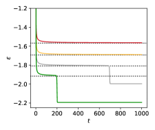
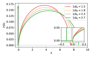
Figure 4: Right panel: energy as a function of time for the set of parameters indicated by small circles in Fig. 2. The horizontal dotted lines correspond to value of the threshold energy ϵthsubscriptitalic-ϵth\epsilon_{\rm th}, as derived both from the Kac-Rice approach in Appendix Sec. A.2.3 and from the large time behaviour of the dynamics in Appendix Sec. B.2.6. Left panel: Eigenvalue distribution of the Hessian of the threshold states for the same set of parameters. When 1/Δ21subscriptΔ21/\Delta_{2} becomes smaller than 222 an isolated eigenvalue appears; it has been highlighted using vertical arrows. Concomitantly, the energy as a function of time first approaches the plateau and eventually departs from it and reaches the energy of the global minimum.

Surfing on saddles: Armed with the dynamical equations, we now confirm the prediction of the threshold (5) based on the Kac-Rice-type of landscape analysis. In the SM we check that the minima trapping the dynamics are indeed the marginally stable ones (t=2𝑡2t=2), see Figs. 7 and 8 in the SM, and we show the energy can be expressed in terms of C𝐶C, R𝑅R and m𝑚m. In the right panel of Fig. 4 we then plot the energy as a function of time obtained from the numerical solution of Eqs. (8-11) for 1/Δ2=1.5,1.9,2.3,2.71subscriptΔ21.51.92.32.71/\Delta_{2}=1.5,1.9,2.3,2.7 and Δp=1subscriptΔ𝑝1\Delta_{p}=1 (same points and colour code of Figs. 2 and 3). For the two smaller values of 1/Δ21subscriptΔ21/\Delta_{2} the energy converges to a plateau value at ϵthsubscriptitalic-ϵth\epsilon_{\rm th} (dotted line), whereas for 1/Δ2=2.3,2.71subscriptΔ22.32.71/\Delta_{2}=2.3,2.7 the energy plateaus close to ϵthsubscriptitalic-ϵth\epsilon_{\rm th} but then eventually drifts away and reaches a lower value, corresponding to the global minimum correlated with the signal. This behaviour can be understood in terms of the spectral properties of the Hessian (6) of the minima trapping the dynamics. In the left panel of Fig. 4 we plot the corresponding density of eigenvalues of \mathcal{H} for the same values of 1/Δ21subscriptΔ21/\Delta_{2} and ΔpsubscriptΔ𝑝\Delta_{p} used in the right panel. This is an illustration of the dynamical phenomenon explained in the previous section: when the signal-to-noise ratio is large enough threshold minima become unstable because a negative eigenvalue, associated to a downward direction toward the signal, emerges. In this case 𝝈(t)𝝈𝑡\boldsymbol{\sigma}(t) first seems to converge to the threshold minima and then, at long times, drifts away along the unstable direction. The larger is the signal-to-noise ratio the more unstable is the downward direction and, hence, the shortest is the intermediate trapping time.

3.2 Gradient-flow Threshold from Dynamical Theory

We now show that the very same prediction (5) for the algorithmic threshold of gradient-flow can be directly obtained analysing the dynamical equations (8-11), without directly using results from the Kac-Rice analysis, thus establishing a firm and novel connection between the behaviour of the gradient-flow algorithm and Kac-Rice landscape approaches.

For small signal-to-noise ratios, when m𝑚m remains zero at all times, the dynamical equations (8-11) are identicall to the well-known one in spin glasses theory, for reviews see [32, 33]. These equations have been studied extensively for decades in statistical physics and a range of results about their behaviour has been established. Here we describe the results which are important for our analysis and devote the SM Sec. B.2 to a more extended presentation. It was shown analytically in [29] that the behaviour of the dynamics at large times is captured by an asymptotic solution of Eqs. (8-11) that verifies several remarkable properties. The ones of interest to us are that for t𝑡t and tsuperscript𝑡t^{\prime} large:

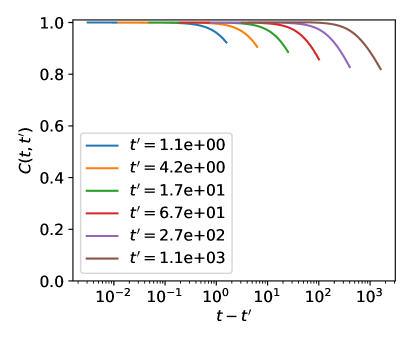
(i) C(t,t)=1𝐶𝑡superscript𝑡1C(t,t^{\prime})=1 when tt𝑡superscript𝑡t-t^{\prime} finite; C(t,t)𝐶𝑡superscript𝑡C(t,t^{\prime}) becomes less than one when tt𝑡superscript𝑡t-t^{\prime} diverges with t𝑡t and tsuperscript𝑡t^{\prime}.

(ii) R(t,t)=RTTI(tt)+Rag(t,t)𝑅𝑡superscript𝑡subscript𝑅TTI𝑡superscript𝑡subscript𝑅ag𝑡superscript𝑡R(t,t^{\prime})=R_{\rm TTI}(t-t^{\prime})+R_{\rm ag}(t,t^{\prime}), where TTI stands for time-translational-invariance, ag stand for aging. Here RTTI(tt)subscript𝑅TTI𝑡superscript𝑡R_{\rm TTI}(t-t^{\prime}) goes to zero on a finite time-scale, whereas Rag(t,t)subscript𝑅ag𝑡superscript𝑡R_{\rm ag}(t,t^{\prime}) varies on timescales diverging with t𝑡t and tsuperscript𝑡t^{\prime}. Moreover, Rag(t,t)subscript𝑅ag𝑡superscript𝑡R_{\rm ag}(t,t^{\prime}) verifies the so called "weak-long term memory" property: for any finite t0subscript𝑡0t_{0}, tt0tRag(t,t′′)𝑑t′′subscriptsuperscript𝑡𝑡subscript𝑡0subscript𝑅ag𝑡superscript𝑡′′differential-dsuperscript𝑡′′\int^{t}_{t-t_{0}}R_{\rm ag}(t,t^{\prime\prime})dt^{\prime\prime} is arbitrarily small. We refer to this function form for R(t,t)𝑅𝑡superscript𝑡R(t,t^{\prime}) as the aging ansatz, adopting the physics terminology.

These properties are confirmed to hold by our numerical solution, see for instance Fig. 9 in the SM. The interpretation of these dynamical properties is that at long times 𝝈(t)𝝈𝑡\boldsymbol{\sigma}(t) decreases in the energy landscape and approaches the marginally stable minima. Concomitantly, dynamics slows down and takes place along the almost flat directions associated to the vanishing eigenvalues of the Hessian.

We remind that in the previous paragraphs we assume null correlation with the signal, m=0𝑚0m=0. In order to find the algorithmic threshold beyond which the gradient-flow develops a positive correlation, we study the instability of the aging solution as a function of the signal-to-noise ratio. Our strategy is to start with an arbitrarily small overlap, m(0)=δ𝑚0𝛿m(0)=\delta, and determine whether it grows at long times thus indicating an instability towards the signal. Since the initial condition for the overlap is uncorrelated with the signal, then, for sufficiently small δ𝛿\delta, C𝐶C and R𝑅R reach their asymptotic form before m𝑚m becomes of order one. We can thus plug the asymptotic aging ansatz for R𝑅R in the dynamical equation for m𝑚m:

ddtm(t)=μ(t)m(t)+Q(m(t))+0tRTTI(tt′′)Q′′(1)m(t′′)𝑑t′′++0tRag(t,t′′)Q′′(Cag(t,t′′))m(t′′)𝑑t′′𝑑𝑑𝑡𝑚𝑡𝜇𝑡𝑚𝑡superscript𝑄𝑚𝑡superscriptsubscript0𝑡subscript𝑅TTI𝑡superscript𝑡′′superscript𝑄′′1𝑚superscript𝑡′′differential-dsuperscript𝑡′′superscriptsubscript0𝑡subscript𝑅ag𝑡superscript𝑡′′superscript𝑄′′subscript𝐶ag𝑡superscript𝑡′′𝑚superscript𝑡′′differential-dsuperscript𝑡′′\begin{split}\frac{d}{dt}m(t)&=-\mu(t)m(t)+Q^{\prime}(m(t))+\int_{0}^{t}R_{\rm TTI}(t-t^{\prime\prime})Q^{\prime\prime}(1)m(t^{\prime\prime})dt^{\prime\prime}+\\ &+\int_{0}^{t}R_{\rm ag}(t,t^{\prime\prime})Q^{\prime\prime}(C_{\rm ag}(t,t^{\prime\prime}))m(t^{\prime\prime})dt^{\prime\prime}\ \end{split} (12)

In the linear approximation the solution has the form m(t)=δexp(Λt)𝑚𝑡𝛿Λ𝑡m(t)=\delta\exp(\Lambda t) and we assume ΛΛ\Lambda arbitrarily small since we want to find the algorithmic threshold where Λ=0Λ0\Lambda=0. The term Q(m(t))superscript𝑄𝑚𝑡Q^{\prime}(m(t)) becomes Q′′(0)m(t)superscript𝑄′′0𝑚𝑡Q^{\prime\prime}(0)m(t). Since m(t)𝑚𝑡m(t) has an arbitrarily slow evolution, whereas RTTI(tt′′)subscript𝑅TTI𝑡superscript𝑡′′R_{\rm TTI}(t-t^{\prime\prime}) relaxes to zero on a finite timescale, the second term of the RHS of eq. (12) simplifies to:

δexp(Λt)Q′′(1)0tRTTI(tt′′)exp(Λ(tt′′))𝑑t′′m(t)Q′′(1)R¯similar-to-or-equals𝛿Λ𝑡superscript𝑄′′1superscriptsubscript0𝑡subscript𝑅TTI𝑡superscript𝑡′′Λ𝑡superscript𝑡′′differential-dsuperscript𝑡′′𝑚𝑡superscript𝑄′′1¯𝑅\delta\exp(\Lambda t)Q^{\prime\prime}(1)\int_{0}^{t}R_{\rm TTI}(t-t^{\prime\prime})\exp(-\Lambda(t-t^{\prime\prime}))dt^{\prime\prime}\simeq m(t)Q^{\prime\prime}(1)\overline{R}

where R¯=0tRTTI(tt′′)𝑑t′′¯𝑅superscriptsubscript0𝑡subscript𝑅TTI𝑡superscript𝑡′′differential-dsuperscript𝑡′′\overline{R}=\int_{0}^{t}R_{\rm TTI}(t-t^{\prime\prime})dt^{\prime\prime} does not depend on t𝑡t (since t𝑡t can be taken arbitrarily large and RTTI(tt′′)subscript𝑅TTI𝑡superscript𝑡′′R_{\rm TTI}(t-t^{\prime\prime}) relaxes to zero on finite time-scales). The contribution of to the last term on (12) reads:

δexp(Λt)0tRag(t,t′′)Q′′(Cag(t,t′′))eΛ(tt′′)dt′′=m(t)0tRag(t,t′′)Q′′(Cag(t,t′′))eΛ(tt′′))dt′′.\begin{split}&\delta\exp(\Lambda t)\!\!\int_{0}^{t}\!\!\!R_{\rm ag}(t,t^{\prime\prime})Q^{\prime\prime}\!(C_{\rm ag}(t,t^{\prime\prime}))e^{\!\!-\Lambda(t-t^{\prime\prime})}dt^{\prime\prime}\!\!=\!m(t)\!\!\int_{0}^{t}\!\!\!R_{\rm ag}(t,t^{\prime\prime})Q^{\prime\prime}\!(C_{\rm ag}(t,t^{\prime\prime}))e^{\!\!-\Lambda(t-t^{\prime\prime})})dt^{\prime\prime}.\end{split}

Using that Q′′(Cag(t,t′′))superscript𝑄′′subscript𝐶ag𝑡superscript𝑡′′Q^{\prime\prime}(C_{\rm ag}(t,t^{\prime\prime})) is bounded by Q′′(1)superscript𝑄′′1Q^{\prime\prime}(1) and that ΛΛ\Lambda cuts-off the integral on a time t01/Λsimilar-tosubscript𝑡01Λt_{0}\sim 1/\Lambda that does not diverge with t𝑡t, we can use the "weak-long term memory" property to conclude that the last term is arbitrarily small compared to m(t)𝑚𝑡m(t) and hence can be neglected with respect to the previous ones. Collecting all the pieces together we find:

ddtm(t)=[μ+Q′′(0)+Q′′(1)R¯]m(t)+O(δ2).𝑑𝑑𝑡𝑚𝑡delimited-[]subscript𝜇superscript𝑄′′0superscript𝑄′′1¯𝑅𝑚𝑡𝑂superscript𝛿2\frac{d}{dt}m(t)=\left[-\mu_{\infty}+Q^{\prime\prime}(0)+Q^{\prime\prime}(1)\overline{R}\right]m(t)+O(\delta^{2})\,. (13)

This is solved by m(t)=δexp(Λt)𝑚𝑡𝛿Λ𝑡m(t)=\delta\exp(\Lambda t) with Λ=μ+Q′′(0)+Q′′(1)R¯,Λsubscript𝜇superscript𝑄′′0superscript𝑄′′1¯𝑅\Lambda=-\mu_{\infty}+Q^{\prime\prime}(0)+Q^{\prime\prime}(1)\overline{R}\,, which therefore justifies a posteriori our assumption of exponential growth. The condition for the instability of the aging solution towards the signal solution is therefore given by

0=μ+Q′′(0)+Q′′(1)R¯.0subscript𝜇superscript𝑄′′0superscript𝑄′′1¯𝑅0=-\mu_{\infty}+Q^{\prime\prime}(0)+Q^{\prime\prime}(1)\overline{R}\,. (14)

From the analysis of the asymptotic aging solution presented in SM Sec. B.2 one finds that μ=2Q′′(1)subscript𝜇2superscript𝑄′′1\mu_{\infty}=2\sqrt{Q^{\prime\prime}(1)} and R¯=1/Q′′(1)¯𝑅1superscript𝑄′′1\overline{R}=1/\sqrt{Q^{\prime\prime}(1)}, therefore obtaining Q′′(0)=Q′′(1)superscript𝑄′′0superscript𝑄′′1Q^{\prime\prime}(0)=\sqrt{Q^{\prime\prime}(1)}. This condition is the same one found from the study of the landscape, and thus leads to the transition line eq. (5).

Acknowledgments

We thank Pierfrancesco Urbani for many related discussions. We acknowledge funding from the ERC under the European Union’s Horizon 2020 Research and Innovation Programme Grant Agreement 714608-SMiLe; from the French National Research Agency (ANR) grant PAIL; and from the Simons Foundation (#454935, Giulio Biroli).

References

  • [1] Kenji Kawaguchi. Deep learning without poor local minima. In Advances in Neural Information Processing Systems, pages 586–594, 2016.
  • [2] Daniel Soudry and Yair Carmon. No bad local minima: Data independent training error guarantees for multilayer neural networks. arXiv preprint arXiv:1605.08361, 2016.
  • [3] Rong Ge, Jason D Lee, and Tengyu Ma. Matrix completion has no spurious local minimum. In Advances in Neural Information Processing Systems, pages 2973–2981, 2016.
  • [4] C Daniel Freeman and Joan Bruna. Topology and geometry of half-rectified network optimization. ICLR 2017, 2017. preprint arXiv:1611.01540.
  • [5] Srinadh Bhojanapalli, Behnam Neyshabur, and Nati Srebro. Global optimality of local search for low rank matrix recovery. In Advances in Neural Information Processing Systems, pages 3873–3881, 2016.
  • [6] Dohyung Park, Anastasios Kyrillidis, Constantine Carmanis, and Sujay Sanghavi. Non-square matrix sensing without spurious local minima via the Burer-Monteiro approach. In Artificial Intelligence and Statistics, pages 65–74, 2017.
  • [7] Simon S Du, Jason D Lee, Yuandong Tian, Aarti Singh, and Barnabas Poczos. Gradient descent learns one-hidden-layer CNN: Don’t be afraid of spurious local minima. In International Conference on Machine Learning, pages 1338–1347, 2018.
  • [8] Rong Ge and Tengyu Ma. On the optimization landscape of tensor decompositions. In Advances in Neural Information Processing Systems, pages 3653–3663, 2017.
  • [9] Rong Ge, Chi Jin, and Yi Zheng. No spurious local minima in nonconvex low rank problems: A unified geometric analysis. In Proceedings of the 34th International Conference on Machine Learning, pages 1233–1242, 2017.
  • [10] Haihao Lu and Kenji Kawaguchi. Depth creates no bad local minima. arXiv preprint arXiv:1702.08580, 2017.
  • [11] Shuyang Ling, Ruitu Xu, and Afonso S Bandeira. On the landscape of synchronization networks: A perspective from nonconvex optimization. arXiv preprint arXiv:1809.11083, 2018.
  • [12] David J Gross and Marc Mézard. The simplest spin glass. Nuclear Physics B, 240(4):431–452, 1984.
  • [13] Yan V Fyodorov. Complexity of random energy landscapes, glass transition, and absolute value of the spectral determinant of random matrices. Physical review letters, 92(24):240601, 2004.
  • [14] Antonio Auffinger, Gérard Ben Arous, and Jiří Černý. Random matrices and complexity of spin glasses. Communications on Pure and Applied Mathematics, 66(2):165–201, 2013.
  • [15] Levent Sagun, V Ugur Guney, Gerard Ben Arous, and Yann LeCun. Explorations on high dimensional landscapes. arXiv preprint arXiv:1412.6615, 2014.
  • [16] Gerard Ben Arous, Song Mei, Andrea Montanari, and Mihai Nica. The landscape of the spiked tensor model. arXiv preprint arXiv:1711.05424, 2017.
  • [17] Iain M Johnstone and Arthur Yu Lu. On consistency and sparsity for principal components analysis in high dimensions. Journal of the American Statistical Association, 104(486):682–693, 2009.
  • [18] Yash Deshpande and Andrea Montanari. Information-theoretically optimal sparse PCA. In Information Theory (ISIT), 2014 IEEE International Symposium on, pages 2197–2201. IEEE, 2014.
  • [19] Emile Richard and Andrea Montanari. A statistical model for tensor PCA. In Advances in Neural Information Processing Systems, pages 2897–2905, 2014.
  • [20] Stefano Sarao Mannelli, Florent Krzakala, Pierfrancesco Urbani, and Lenka Zdeborova. Passed & spurious: Descent algorithms and local minima in spiked matrix-tensor models. In International Conference on Machine Learning, pages 4333–4342, 2019.
  • [21] Stefano Sarao Mannelli, Giulio Biroli, Chiara Cammarota, Florent Krzakala, Pierfrancesco Urbani, and Lenka Zdeborová. Marvels and pitfalls of the langevin algorithm in noisy high-dimensional inference. arXiv preprint arXiv:1812.09066, 2018.
  • [22] Valentina Ros, Gerard Ben Arous, Giulio Biroli, and Chiara Cammarota. Complex energy landscapes in spiked-tensor and simple glassy models: Ruggedness, arrangements of local minima, and phase transitions. Physical Review X, 9(1):011003, 2019.
  • [23] Jinho Baik, Gérard Ben Arous, Sandrine Péché, et al. Phase transition of the largest eigenvalue for nonnull complex sample covariance matrices. The Annals of Probability, 33(5):1643–1697, 2005.
  • [24] A Crisanti, H Horner, and H-J Sommers. The spherical p𝑝p-spin interaction spin-glass model. Zeitschrift für Physik B Condensed Matter, 92(2):257–271, 1993.
  • [25] Leticia F Cugliandolo and Jorge Kurchan. Analytical solution of the off-equilibrium dynamics of a long-range spin-glass model. Physical Review Letters, 71(1):173, 1993.
  • [26] Gerard Ben Arous, Amir Dembo, and Alice Guionnet. Cugliandolo-Kurchan equations for dynamics of spin-glasses. Probability theory and related fields, 136(4):619–660, 2006.
  • [27] Tommaso Castellani and Andrea Cavagna. Spin glass theory for pedestrians. Journal of Statistical Mechanics: Theory and Experiment, 2005:P05012, 2005.
  • [28] Andrea Crisanti and H-J Sommers. The spherical p-spin interaction spin glass model: the statics. Zeitschrift für Physik B Condensed Matter, 87(3):341–354, 1992.
  • [29] Leticia F Cugliandolo and Jorge Kurchan. On the out-of-equilibrium relaxation of the Sherrington-Kirkpatrick model. Journal of Physics A: Mathematical and General, 27(17):5749, 1994.
  • [30] Leticia F Cugliandolo and Jorge Kurchan. Weak ergodicity breaking in mean-field spin-glass models. Philosophical Magazine B, 71(4):501–514, 1995.
  • [31] Pompiliu Manuel Zamfir. Limiting dynamics for spherical models of spin glasses with magnetic field. arXiv preprint arXiv:0806.3519, 2008.
  • [32] Jean-Philippe Bouchaud, Leticia F Cugliandolo, Jorge Kurchan, and Marc Mézard. Out of equilibrium dynamics in spin-glasses and other glassy systems. Spin glasses and random fields, pages 161–223, 1998.
  • [33] Leticia F Cugliandolo. Course 7: Dynamics of glassy systems. In Slow Relaxations and nonequilibrium dynamics in condensed matter, pages 367–521. Springer, 2003.
  • [34] Eliran Subag. The complexity of spherical p𝑝p-spin models—a second moment approach. The Annals of Probability, 45(5):3385–3450, 2017.
  • [35] Robert J Adler and Jonathan E Taylor. Random fields and geometry. Springer Science & Business Media, 2009.
  • [36] Andrea Crisanti and Luca Leuzzi. Spherical 2+ p spin-glass model: An exactly solvable model for glass to spin-glass transition. Physical review letters, 93(21):217203, 2004.
  • [37] Gerard Ben Arous, Reza Gheissari, and Aukosh Jagannath. Algorithmic thresholds for tensor PCA. arXiv preprint arXiv:1808.00921, 2018.
  • [38] A Barrat. The p-spin spherical spin glass model. arXiv preprint cond-mat/9701031, 1997.
  • [39] Jorge Kurchan and Laurent Laloux. Phase space geometry and slow dynamics. Journal of Physics A: Mathematical and General, 29(9):1929, 1996.
  • [40] Florent Krzakala and Lenka Zdeborová. Performance of simulated annealing in p-spin glasses. In Journal of Physics: Conference Series, volume 473, page 012022. IOP Publishing, 2013.
  • [41] Guilhem Semerjian, Leticia F Cugliandolo, and Andrea Montanari. On the stochastic dynamics of disordered spin models. Journal of statistical physics, 115(1-2):493–530, 2004.

Appendix A Kac-Rice method

A.1 Summary of the Kac-Rice complexity

Refer to caption
Refer to caption
Refer to caption
Refer to caption
Refer to caption
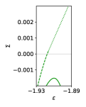
Figure 5: Curves of the complexity of critical points, dotted and dashed curves from Eq. (17), and of minima, full curve from Eq. (19), at overlap value m=0𝑚0m=0 at fixed Δp=1.0subscriptΔ𝑝1.0\Delta_{p}=1.0 for different Δ2subscriptΔ2\Delta_{2}. The figure shows qualitatively the same features as Fig. 3, but displays the full positive part of the complexity for the four cases discussed in the main text, 1/Δ2{1.5, 1.9, 2.3, 2.7}1subscriptΔ21.51.92.32.71/\Delta_{2}\in\{1.5,\,1.9,\,2.3,\,2.7\}. Zooms of the curves of the annealed complexity of critical points and minima when they cross zero at negative loss are in the panels labelled from (a) to (d) for increasing 1/Δ21subscriptΔ21/\Delta_{2}.

In this section we introduce the Kac-Rice formula and we show how to reduce it to an explicit expression for the spiked matrix-tensor model. The Kac-Rice formula evaluates the expected number of critical points of a rough function subject to a number of conditions. For an inference problem it is interesting to focus on the expected number of critical points constrained to have of given loss and a given overlap with the ground truth. For convenience reasons we consider the rescaled loss (𝝈)=N(𝝈)𝝈𝑁𝝈\mathcal{L}(\boldsymbol{\sigma})=N\ell(\boldsymbol{\sigma}). The Kac-Rice formula then reads

𝔼η[𝒩(ϵ,m|Θ)]=𝕊N1δ(𝝈,𝝈m)𝔼η[|det||=Nϵ,i=0i,λmin>0]××ϕ,i(𝝈,𝟎,ϵ)d𝝈,subscript𝔼𝜂delimited-[]𝒩italic-ϵconditional𝑚Θsubscriptsuperscript𝕊𝑁1𝛿𝝈superscript𝝈𝑚subscript𝔼𝜂delimited-[]ketformulae-sequence𝑁italic-ϵsubscript𝑖0for-all𝑖subscript𝜆0subscriptitalic-ϕsubscript𝑖𝝈0italic-ϵ𝑑𝝈\begin{split}\mathbb{E}_{\eta}[\mathcal{N}(\epsilon,m|\Theta)]&=\int_{\mathbb{S}^{N-1}}\delta\left(\langle\boldsymbol{\sigma},\boldsymbol{\sigma}^{*}\rangle-m\right)\mathbb{E}_{\eta}\left[|\det\mathcal{H}|\Big{|}\mathcal{L}=N\,\epsilon,\partial_{i}\mathcal{L}=0\ \forall i,\lambda_{\min}>0\right]\times\\ &\times\phi_{\mathcal{L},\,\partial_{i}\mathcal{L}}(\boldsymbol{\sigma},\boldsymbol{0},\epsilon)d\boldsymbol{\sigma}\,,\end{split} (15)

where η𝜂\eta represents the noise in the problem, ΘΘ\Theta the parameters and ϕitalic-ϕ\phi the joint probability density of the loss and its gradient.

The quantity of interest is the density of the logarithm of the number of critical points log𝒩(ϵ,m|Θ)/N𝒩italic-ϵconditional𝑚Θ𝑁\log\mathcal{N}(\epsilon,m|\Theta)/N. It should be noted that, since the random variable representing the number of critical point fluctuates at the exponential scale, a correct estimation of the expected value of this quantity is not log𝔼η[𝒩(ϵ,m|Θ)]subscript𝔼𝜂delimited-[]𝒩italic-ϵconditional𝑚Θ\log\mathbb{E}_{\eta}[\mathcal{N}(\epsilon,m|\Theta)], as it would be immediately obtained by using the result of the Kac-Rice formula [20], but 𝔼η[log𝒩(ϵ,m|Θ)]subscript𝔼𝜂delimited-[]𝒩italic-ϵconditional𝑚Θ\mathbb{E}_{\eta}[\log\mathcal{N}(\epsilon,m|\Theta)]. These two quantities are called respectively annealed and quenched complexities. Using Jensen inequality one observes that the annealed complexity is just an upper bound of the quenched one. However, for mathematical convenience most of the studies have been focused on the former. Eventually the second moment of the number of critical points has been evaluated [34], by an extension of the Kac-Rice formula to higher moments [35], just to prove that the two are equivalent in some models [34]. The quenched complexity has been evaluated in a related model in a non rigorous way by studying the n𝑛n-th moment and applying replica trick, the so-called replicated Kac-Rice [22]. Given a random variable Y𝑌Y replica trick says

𝔼η[logY]=limn0+𝔼η[Yn]1nsubscript𝔼𝜂delimited-[]𝑌subscript𝑛superscript0subscript𝔼𝜂delimited-[]superscript𝑌𝑛1𝑛\mathbb{E}_{\eta}[\log Y]=\lim_{n\rightarrow 0^{+}}\frac{\mathbb{E}_{\eta}[Y^{n}]-1}{n} (16)

but instead of considering an arbitrary n+𝑛superscriptn\in\mathbb{R}^{+}, the study is done using n𝑛n\in\mathbb{N} and performing an analytic continuation of the result to 0+superscript00^{+}. The replica trick has already been used in a plethora of applications and, although not rigorous, it was found correct in all naturally motivated cases that have been later approached by other techniques. An important mathematical literature has developed in order to understand the method.

In the next section we sketch the derivation of the quenched Kac-Rice and we provide all the information to determine the annealed one. Since the threshold is determined considering the configuration with arbitrarily small overlap m1much-less-than𝑚1m\ll 1, we focus on that case. Remarkably we found that as m0𝑚0m\rightarrow 0 the quenched complexity computed within the replica symmetric (RS) approximation is equal to the annealed one111We expect the RS approximation to be correct for p=3𝑝3p=3 in the whole (Δp,1/Δ2)subscriptΔ𝑝1subscriptΔ2(\Delta_{p},1/\Delta_{2}) phase diagram, and hence that quenched and annealed complexities coincide. For p>3𝑝3p>3, results from replica theory [36] suggest that one needs to go beyond the RS approximation at least in some parts of the phase diagram.. We show that the corresponding Hessian is Eq. (6) in the main text, i.e. it is proportional to a GOE translated by t𝑡t and perturbed by a rank n𝑛n perturbation of strength θ𝜃\theta that in the annealed case is of rank 111. Thus we find that the complexity for the stationary points is [20]

Σasta(m,ϵ|Δp,Δ2)=maxϵp,ϵ2s.t. ϵp+ϵ2=ϵ12logQ′′(1)Q(1)+12log(1m2)12(Q′′(m))2Q(1)(1m2)+pΔp2(ϵp+mppΔp)2Δ2(ϵ2+m22Δ2)2+Φ(t),\begin{split}\Sigma_{a}^{\text{sta}}(m,\epsilon|\Delta_{p},\Delta_{2})&=\max_{\begin{subarray}{c}\epsilon_{p},\epsilon_{2}\\ \text{s.t. }\epsilon_{p}+\epsilon_{2}=\epsilon\end{subarray}}\frac{1}{2}\log\frac{Q^{\prime\prime}(1)}{Q^{\prime}(1)}+\frac{1}{2}\log(1-m^{2})-\frac{1}{2}\frac{\left(Q^{\prime\prime}(m)\right)^{2}}{Q^{\prime}(1)}(1-m^{2})+\\ &-\frac{p\Delta_{p}}{2}\left(\epsilon_{p}+\frac{m^{p}}{p\Delta_{p}}\right)^{2}-\Delta_{2}\left(\epsilon_{2}+\frac{m^{2}}{2\Delta_{2}}\right)^{2}+\Phi(t),\end{split} (17)

with

Φ(t)={t24if |t|2t24+log(t241+|t|2)|t|4t24otherwiseΦ𝑡casesotherwisesuperscript𝑡24if 𝑡2otherwisesuperscript𝑡24superscript𝑡241𝑡2𝑡4superscript𝑡24otherwise\Phi(t)=\begin{cases}&\frac{t^{2}}{4}\quad\quad\text{if }|t|\leq 2\\ &\frac{t^{2}}{4}+\log\left(\sqrt{\frac{t^{2}}{4}-1}+\frac{|t|}{2}\right)-\frac{|t|}{4}\sqrt{t^{2}-4}\quad\quad\text{otherwise}\end{cases} (18)

and t=(pϵp+2ϵ2)/Q′′(1)𝑡𝑝subscriptitalic-ϵ𝑝2subscriptitalic-ϵ2superscript𝑄′′1t=-\left(p\epsilon_{p}+2\epsilon_{2}\right)/\sqrt{Q^{\prime\prime}(1)} as already introduced in the main text. Finally studying the eigenvalue of the Hessian to constrain them in the positive semi-axis, we find the complexity of minima [20]

Σa(m,ϵ|Δp,Δ2)=Σasta(m,ϵp,ϵ2|Δp,Δ2)L(θ,t).subscriptΣ𝑎𝑚conditionalitalic-ϵsubscriptΔ𝑝subscriptΔ2superscriptsubscriptΣ𝑎sta𝑚subscriptitalic-ϵ𝑝conditionalsubscriptitalic-ϵ2subscriptΔ𝑝subscriptΔ2𝐿𝜃𝑡\Sigma_{a}(m,\epsilon|\Delta_{p},\Delta_{2})=\Sigma_{a}^{\text{sta}}(m,\epsilon_{p},\epsilon_{2}|\Delta_{p},\Delta_{2})-L(\theta,t)\,. (19)

with

L(θ,t)={14θ+1θty24𝑑yθ2(t(θ+1θ))+t2(θ+1θ)28θ>1, 2t<θ2+1θt<20otherwise.𝐿𝜃𝑡casesotherwiseformulae-sequence14superscriptsubscript𝜃1𝜃𝑡superscript𝑦24differential-d𝑦𝜃2𝑡𝜃1𝜃superscript𝑡2superscript𝜃1𝜃28𝜃12𝑡superscript𝜃21𝜃otherwise𝑡2otherwise0otherwise.L(\theta,t)=\begin{cases}&\frac{1}{4}\int_{\theta+\frac{1}{\theta}}^{t}\sqrt{y^{2}-4}dy-\frac{\theta}{2}\left(t-\left(\theta+\frac{1}{\theta}\right)\right)+\frac{t^{2}-\left(\theta+\frac{1}{\theta}\right)^{2}}{8}\quad\theta>1,\;2\leq t<\frac{\theta^{2}+1}{\theta}\\ &\infty\quad\quad t<2\\ &0\quad\quad\text{otherwise.}\\ \end{cases} (20)

and θ=Q′′(m)(1m2)/Q′′(1)𝜃superscript𝑄′′𝑚1superscript𝑚2superscript𝑄′′1\theta=Q^{\prime\prime}(m)\,(1-m^{2})/\sqrt{Q^{\prime\prime}(1)}. In Fig. 5, we show the two complexities of the stationary points and of the minima in the parameter space discussed in the main text with discontinuous lines Eq. (17) and full lines Eq. (19), respectively. A positive complexity means an exponential number of critical points (minima). The region where exponentially many minima appear is highlighted in the small figures, showing the coexistence of exponentially many minima and saddles.

A.2 Derivation of the quenched complexity

We proceed with the computation of the quenched Kac-Rice complexity for the spiked matrix-tensor model, using replicated Kac-Rice prescription for the spiked pure-tensor model [22]. This implies, following replica trick Eq. (16), the evaluation of the n𝑛n-th moment of number of minima using Kac-Rice formula which is given by [35]

𝔼η[𝒩(ϵ,m|Θ)n]=𝕊N1𝕊N1𝔼η[(a=1n|det[𝝈a]|)|b,c[𝝈b]=Nϵ,i[𝝈c]=0i,λmin>0]×ϕ,i({𝝈a},𝟎,ϵ)a=1nδ(𝝈a,𝝈m)d𝝈a.subscript𝔼𝜂delimited-[]𝒩superscriptitalic-ϵconditional𝑚Θ𝑛subscriptsuperscript𝕊𝑁1subscriptsuperscript𝕊𝑁1subscript𝔼𝜂delimited-[]superscriptsubscriptproduct𝑎1𝑛delimited-[]superscript𝝈𝑎ketformulae-sequencefor-all𝑏𝑐delimited-[]superscript𝝈𝑏𝑁italic-ϵsubscript𝑖delimited-[]superscript𝝈𝑐0for-all𝑖subscript𝜆0subscriptitalic-ϕsubscript𝑖superscript𝝈𝑎0italic-ϵsuperscriptsubscriptproduct𝑎1𝑛𝛿superscript𝝈𝑎superscript𝝈𝑚𝑑superscript𝝈𝑎\begin{split}\mathbb{E}_{\eta}[\mathcal{N}(\epsilon,m|\Theta)^{n}]\!&=\int_{\mathbb{S}^{N-1}}\cdots\int_{\mathbb{S}^{N-1}}\mathbb{E}_{\eta}\left[\left(\prod_{a=1}^{n}\left|\det\mathcal{H}[\boldsymbol{\sigma}^{a}]\right|\right)\Bigg{|}\forall b,c\ \mathcal{L}[\boldsymbol{\sigma}^{b}]=N\epsilon,\partial_{i}\mathcal{L}[\boldsymbol{\sigma}^{c}]=0\ \forall i,\lambda_{\min}\!\!>0\right]\\ &\times\phi_{\mathcal{L},\,\partial_{i}\mathcal{L}}\left(\{\boldsymbol{\sigma}^{a}\},\boldsymbol{0},\epsilon\right)\prod_{a=1}^{n}\delta\left(\langle\boldsymbol{\sigma}^{a},\boldsymbol{\sigma}^{*}\rangle-m\right)d\boldsymbol{\sigma}^{a}\,.\end{split} (21)

Where ϕitalic-ϕ\phi is the joint probability density of the loss and its gradients evaluated on the n𝑛n replicated configurations. We hereby sketch the main computation steps and present the results that are the most relevant for the theory presented in this paper, i.e. for m=0𝑚0m=0. The details of the computation and further results for m>0𝑚0m>0 will be presented in a dedicated work elsewhere.

It is convenient to consider free variables on Nsuperscript𝑁\mathbb{R}^{N} and constrain them using a Lagrange multiplier γ𝛾\gamma. Thus (𝝈a)(𝝈a)γ2(i(σia)21)maps-tosuperscript𝝈𝑎superscript𝝈𝑎𝛾2subscript𝑖superscriptsubscriptsuperscript𝜎𝑎𝑖21\mathcal{L}(\boldsymbol{\sigma}^{a})\mapsto\mathcal{L}(\boldsymbol{\sigma}^{a})-\frac{\gamma}{2}\left(\sum_{i}(\sigma^{a}_{i})^{2}-1\right). Using the fact that the gradient must be zero on the sphere, i.e. that i(𝝈a)γσia=0isubscript𝑖superscript𝝈𝑎𝛾subscriptsuperscript𝜎𝑎𝑖0for-all𝑖\nabla_{i}\mathcal{L}(\boldsymbol{\sigma}^{a})-\gamma\,\sigma^{a}_{i}=0\ \ \forall i, we obtain a simple expression for the multiplier: γ=(𝝈a),𝝈a𝛾bold-∇superscript𝝈𝑎superscript𝝈𝑎\gamma=\langle\boldsymbol{\nabla}\mathcal{L}(\boldsymbol{\sigma}^{a}),\boldsymbol{\sigma}^{a}\rangle. Moreover by separating the two terms in the loss that represent the contribution of the two channels, =p+2subscript𝑝subscript2\mathcal{L}=\mathcal{L}_{p}+\mathcal{L}_{2}, we define p=Nϵpsubscript𝑝𝑁subscriptitalic-ϵ𝑝\mathcal{L}_{p}=N\epsilon_{p} and 2=Nϵ2subscript2𝑁subscriptitalic-ϵ2\mathcal{L}_{2}=N\epsilon_{2} so to obtain for the multiplier the even simpler equation γ=pϵp+2ϵ2𝛾𝑝subscriptitalic-ϵ𝑝2subscriptitalic-ϵ2\gamma=p\epsilon_{p}+2\epsilon_{2}. To take advantage of this simple formula, in the following we work with the contributions of the two channels to the loss function separately and we impose the constraint on their sum, Nϵ=N(ϵp+ϵ2)𝑁italic-ϵ𝑁subscriptitalic-ϵ𝑝subscriptitalic-ϵ2N\epsilon=N(\epsilon_{p}+\epsilon_{2}), only at the end.

The use of Cartesian coordinates allows us to evaluate easily the moments and covariances by means of standard derivatives.

𝔼η[[𝝈a]]=NQ(𝝈a,𝝈),subscript𝔼𝜂delimited-[]delimited-[]superscript𝝈𝑎𝑁𝑄superscript𝝈𝑎superscript𝝈\displaystyle\mathbb{E}_{\eta}\left[\mathcal{L}[\boldsymbol{\sigma}^{a}]\right]=-NQ(\langle\boldsymbol{\sigma}^{a},\boldsymbol{\sigma}^{*}\rangle)\,, (22)
Cov[[𝝈a],[𝝈b]]=NQ(𝝈a,𝝈b).Covdelimited-[]superscript𝝈𝑎delimited-[]superscript𝝈𝑏𝑁𝑄superscript𝝈𝑎superscript𝝈𝑏\displaystyle\text{Cov}\left[\mathcal{L}[\boldsymbol{\sigma}^{a}],\mathcal{L}[\boldsymbol{\sigma}^{b}]\right]=N\,Q\left(\langle\boldsymbol{\sigma}^{a},\boldsymbol{\sigma}^{b}\rangle\right)\,. (23)

Taking derivatives of these equation gives all the covariances of loss, gradient and Hessian. For instance, we can easily see that the covariance of the Hessian is given by:

4σiaσjaσkbσlbCov[[𝝈a],[𝝈b]]N=Q′′′′(𝝈a,𝝈b)𝝈b,𝒆ia𝝈b,𝒆ja𝝈a,𝒆kb𝝈a,𝒆lb++Q′′′(𝝈a,𝝈b)(𝒆ia,𝒆kb𝝈b,𝒆ja𝝈a,𝒆lb+𝒆ja,𝒆kb𝝈b,𝒆ia𝝈a,𝒆lb+𝒆ia,𝒆lb𝝈b,𝒆ja𝝈a,𝒆kb++𝒆ja,𝒆lb𝝈b,𝒆ia𝝈a,𝒆kb)+Q′′(𝝈a,𝝈b)(𝒆ia,𝒆kb𝒆ja,𝒆lb+𝒆ia,𝒆lb𝒆ja,𝒆kb),superscript4subscriptsuperscript𝜎𝑎𝑖subscriptsuperscript𝜎𝑎𝑗subscriptsuperscript𝜎𝑏𝑘subscriptsuperscript𝜎𝑏𝑙Covdelimited-[]superscript𝝈𝑎delimited-[]superscript𝝈𝑏𝑁superscript𝑄′′′′superscript𝝈𝑎superscript𝝈𝑏superscript𝝈𝑏superscriptsubscript𝒆𝑖𝑎superscript𝝈𝑏superscriptsubscript𝒆𝑗𝑎superscript𝝈𝑎superscriptsubscript𝒆𝑘𝑏superscript𝝈𝑎superscriptsubscript𝒆𝑙𝑏superscript𝑄′′′superscript𝝈𝑎superscript𝝈𝑏superscriptsubscript𝒆𝑖𝑎superscriptsubscript𝒆𝑘𝑏superscript𝝈𝑏superscriptsubscript𝒆𝑗𝑎superscript𝝈𝑎superscriptsubscript𝒆𝑙𝑏superscriptsubscript𝒆𝑗𝑎superscriptsubscript𝒆𝑘𝑏superscript𝝈𝑏superscriptsubscript𝒆𝑖𝑎superscript𝝈𝑎superscriptsubscript𝒆𝑙𝑏superscriptsubscript𝒆𝑖𝑎superscriptsubscript𝒆𝑙𝑏superscript𝝈𝑏superscriptsubscript𝒆𝑗𝑎superscript𝝈𝑎superscriptsubscript𝒆𝑘𝑏superscriptsubscript𝒆𝑗𝑎superscriptsubscript𝒆𝑙𝑏superscript𝝈𝑏superscriptsubscript𝒆𝑖𝑎superscript𝝈𝑎superscriptsubscript𝒆𝑘𝑏superscript𝑄′′superscript𝝈𝑎superscript𝝈𝑏superscriptsubscript𝒆𝑖𝑎superscriptsubscript𝒆𝑘𝑏superscriptsubscript𝒆𝑗𝑎superscriptsubscript𝒆𝑙𝑏superscriptsubscript𝒆𝑖𝑎superscriptsubscript𝒆𝑙𝑏superscriptsubscript𝒆𝑗𝑎superscriptsubscript𝒆𝑘𝑏\begin{split}&\frac{\partial^{4}}{\partial\sigma^{a}_{i}\partial\sigma^{a}_{j}\partial\sigma^{b}_{k}\partial\sigma^{b}_{l}}\frac{\text{Cov}\left[\mathcal{L}[\boldsymbol{\sigma}^{a}],\mathcal{L}[\boldsymbol{\sigma}^{b}]\right]}{N}=Q^{\prime\prime\prime\prime}\left(\langle\boldsymbol{\sigma}^{a},\boldsymbol{\sigma}^{b}\rangle\right)\langle\boldsymbol{\sigma}^{b},\boldsymbol{e}_{i}^{a}\rangle\langle\boldsymbol{\sigma}^{b},\boldsymbol{e}_{j}^{a}\rangle\langle\boldsymbol{\sigma}^{a},\boldsymbol{e}_{k}^{b}\rangle\langle\boldsymbol{\sigma}^{a},\boldsymbol{e}_{l}^{b}\rangle+\\ &\,+Q^{\prime\prime\prime}\left(\langle\boldsymbol{\sigma}^{a},\boldsymbol{\sigma}^{b}\rangle\right)\!\Big{(}\langle\boldsymbol{e}_{i}^{a},\boldsymbol{e}_{k}^{b}\rangle\langle\boldsymbol{\sigma}^{b},\boldsymbol{e}_{j}^{a}\rangle\langle\boldsymbol{\sigma}^{a},\boldsymbol{e}_{l}^{b}\rangle\!+\!\langle\boldsymbol{e}_{j}^{a},\boldsymbol{e}_{k}^{b}\rangle\langle\boldsymbol{\sigma}^{b},\boldsymbol{e}_{i}^{a}\rangle\langle\boldsymbol{\sigma}^{a},\boldsymbol{e}_{l}^{b}\rangle\!+\!\langle\boldsymbol{e}_{i}^{a},\boldsymbol{e}_{l}^{b}\rangle\langle\boldsymbol{\sigma}^{b},\boldsymbol{e}_{j}^{a}\rangle\langle\boldsymbol{\sigma}^{a},\boldsymbol{e}_{k}^{b}\rangle+\\ &\,+\langle\boldsymbol{e}_{j}^{a},\boldsymbol{e}_{l}^{b}\rangle\langle\boldsymbol{\sigma}^{b},\boldsymbol{e}_{i}^{a}\rangle\langle\boldsymbol{\sigma}^{a},\boldsymbol{e}_{k}^{b}\rangle\Big{)}+Q^{\prime\prime}\left(\langle\boldsymbol{\sigma}^{a},\boldsymbol{\sigma}^{b}\rangle\right)\Big{(}\langle\boldsymbol{e}_{i}^{a},\boldsymbol{e}_{k}^{b}\rangle\langle\boldsymbol{e}_{j}^{a},\boldsymbol{e}_{l}^{b}\rangle+\langle\boldsymbol{e}_{i}^{a},\boldsymbol{e}_{l}^{b}\rangle\langle\boldsymbol{e}_{j}^{a},\boldsymbol{e}_{k}^{b}\rangle\Big{)}\,,\end{split} (24)

where {𝒆ia}isubscriptsubscriptsuperscript𝒆𝑎𝑖𝑖\{\boldsymbol{e}^{a}_{i}\}_{i} and {𝒆kb}ksubscriptsubscriptsuperscript𝒆𝑏𝑘𝑘\{\boldsymbol{e}^{b}_{k}\}_{k} are the reference frames associated to replica a𝑎a and b𝑏b respectively.

Remark 1 (annealed Hessian)

In particular notice that if n=1𝑛1n=1 there is only one replica and using an orthogonal basis where the N𝑁N-th direction is aligned with the replica and projecting on the sphere by discarding the last coordinates we obtain a simple expression:

1NCov[ij[𝝈],kl[𝝈]]=Q′′(1)(δikδjl+δilδjk)1𝑁Covsubscript𝑖𝑗delimited-[]𝝈subscript𝑘𝑙delimited-[]𝝈superscript𝑄′′1subscript𝛿𝑖𝑘subscript𝛿𝑗𝑙subscript𝛿𝑖𝑙subscript𝛿𝑗𝑘\frac{1}{N}\text{Cov}\left[\mathcal{H}_{ij}[\boldsymbol{\sigma}],\mathcal{H}_{kl}[\boldsymbol{\sigma}]\right]=Q^{\prime\prime}(1)\left(\delta_{ik}\delta_{jl}+\delta_{il}\delta_{jk}\right) (25)

with the delta𝑑𝑒𝑙𝑡𝑎delta representing Kronecker’s deltas. This is the expression of a GOE. We can as well compute the mean deriving twice in the i𝑖i-th and j𝑗j-th coordinate. Following [16] we make another convenient choice for the basis imposing that the signal lies in the space spanned by the 𝐞1subscript𝐞1\boldsymbol{e}_{1} and 𝐞N=𝛔subscript𝐞𝑁𝛔\boldsymbol{e}_{N}=\boldsymbol{\sigma}. This gives,

1N𝔼[ij[𝝈]]=Q′′(𝝈a,𝝈)𝝈,𝒆i𝝈,𝒆j=Q′′(𝝈a,𝝈)𝝈,𝒆i𝝈,𝒆jδi1δj11𝑁𝔼delimited-[]subscript𝑖𝑗delimited-[]𝝈superscript𝑄′′superscript𝝈𝑎superscript𝝈superscript𝝈subscript𝒆𝑖superscript𝝈subscript𝒆𝑗superscript𝑄′′superscript𝝈𝑎superscript𝝈superscript𝝈subscript𝒆𝑖superscript𝝈subscript𝒆𝑗subscript𝛿𝑖1subscript𝛿𝑗1\frac{1}{N}\mathbb{E}\left[\mathcal{H}_{ij}[\boldsymbol{\sigma}]\right]=Q^{\prime\prime}(\langle\boldsymbol{\sigma}^{a},\boldsymbol{\sigma}^{*}\rangle)\,\langle\boldsymbol{\sigma}^{*},\boldsymbol{e}_{i}\rangle\langle\boldsymbol{\sigma}^{*},\boldsymbol{e}_{j}\rangle=Q^{\prime\prime}(\langle\boldsymbol{\sigma}^{a},\boldsymbol{\sigma}^{*}\rangle)\,\langle\boldsymbol{\sigma}^{*},\boldsymbol{e}_{i}\rangle\langle\boldsymbol{\sigma}^{*},\boldsymbol{e}_{j}\rangle\delta_{i1}\delta_{j1} (26)

that, when m=0𝑚0m=0, equals

1N𝔼[[𝝈]]=Q′′(0)𝒆1𝒆1T.1𝑁𝔼delimited-[]delimited-[]𝝈superscript𝑄′′0subscript𝒆1superscriptsubscript𝒆1𝑇\frac{1}{N}\mathbb{E}\left[\mathcal{H}[\boldsymbol{\sigma}]\right]=Q^{\prime\prime}(0)\,\boldsymbol{e}_{1}\boldsymbol{e}_{1}^{T}\,. (27)

Wrapping together Eq. (25), Eq. (27) and the expression for the Langrange multiplier that acts as a translation, we obtain the Hessian presented in the main text Eq. (6). Observe, however, that the Hessian in which we are interested in is not the simple Hessian of the loss but rather the Hessian of the loss conditioned to a given loss and a given gradient. Using Eq. (23) to compute the covariance of Hessian and loss, and of Hessian and gradient under this basis, we can observe that these random variables are unconditioned. Thus the conditioning does not affect the distribution of the Hessian of the loss and therefore Eq. (6) is recovered.

Eq. (22) and Eq. (23) are basic ingredients required to continue with the analysis. In the next two sections we first compute the joint density of the loss and its gradient, and second compute the expected value of the determinant of the Hessians. In the final section we put together the results obtaining the complexities already presented in the summary A.1.

A.2.1 Joint probability density.

In order to evaluate the joint probability density ϕitalic-ϕ\phi we focus on the covariance matrix of the loss and its gradient, that using Eq. (23) is given by:

1N[𝑪,]a,b=[Q′′(𝝈a,𝝈b)𝝈a𝝈b+Q(𝝈a,𝝈b)𝕀NQ(𝝈a,𝝈b)𝝈b,TQ(𝝈a,𝝈b)𝝈aQ(𝝈a,𝝈b)].1𝑁superscriptdelimited-[]subscript𝑪𝑎𝑏matrixtensor-productsuperscript𝑄′′superscript𝝈𝑎superscript𝝈𝑏superscript𝝈𝑎superscript𝝈𝑏superscript𝑄superscript𝝈𝑎superscript𝝈𝑏subscript𝕀𝑁superscript𝑄superscript𝝈𝑎superscript𝝈𝑏superscript𝝈𝑏𝑇superscript𝑄superscript𝝈𝑎superscript𝝈𝑏superscript𝝈𝑎𝑄superscript𝝈𝑎superscript𝝈𝑏\frac{1}{N}\left[\boldsymbol{C}_{\mathcal{L},\nabla\mathcal{L}}\right]^{a,b}=\begin{bmatrix}Q^{\prime\prime}\left(\langle\boldsymbol{\sigma}^{a},\boldsymbol{\sigma}^{b}\rangle\right)\boldsymbol{\sigma}^{a}\otimes\boldsymbol{\sigma}^{b}+Q^{\prime}\left(\langle\boldsymbol{\sigma}^{a},\boldsymbol{\sigma}^{b}\rangle\right)\mathbb{I}_{N}&Q^{\prime}\left(\langle\boldsymbol{\sigma}^{a},\boldsymbol{\sigma}^{b}\rangle\right)\boldsymbol{\sigma}^{b,T}\\ Q^{\prime}\left(\langle\boldsymbol{\sigma}^{a},\boldsymbol{\sigma}^{b}\rangle\right)\boldsymbol{\sigma}^{a}&Q\left(\langle\boldsymbol{\sigma}^{a},\boldsymbol{\sigma}^{b}\rangle\right)\end{bmatrix}\,. (28)

The joint density corresponds to the probability of observing a zero gradient on the sphere and a given loss, (γ𝝈T,ϵ)Tsuperscript𝛾superscript𝝈𝑇italic-ϵ𝑇(\gamma\,\boldsymbol{\sigma}^{T},\epsilon)^{T}, in the multivariate Gaussian variable (T,)Tsuperscriptbold-∇superscript𝑇𝑇(\boldsymbol{\nabla}\mathcal{L}^{T},\mathcal{L})^{T}. Thus taking into account the first moments of loss and gradient, obtained from Eq. (22), we define the auxiliary vector

[𝝁(ϵp,ϵ2)]a=((pϵp+2ϵ2)𝝈a,T+Q(𝝈a,𝝈)𝝈,T,ϵ+Q(𝝈a,𝝈))T.superscriptdelimited-[]𝝁subscriptitalic-ϵ𝑝subscriptitalic-ϵ2𝑎superscript𝑝subscriptitalic-ϵ𝑝2subscriptitalic-ϵ2superscript𝝈𝑎𝑇superscript𝑄superscript𝝈𝑎superscript𝝈superscript𝝈𝑇italic-ϵ𝑄superscript𝝈𝑎superscript𝝈𝑇[\boldsymbol{\mu}(\epsilon_{p},\epsilon_{2})]^{a}=\left((p\epsilon_{p}+2\epsilon_{2})\boldsymbol{\sigma}^{a,T}+Q^{\prime}(\langle\boldsymbol{\sigma}^{a},\boldsymbol{\sigma}^{*}\rangle)\boldsymbol{\sigma}^{*,T},\ \epsilon+Q(\langle\boldsymbol{\sigma}^{a},\boldsymbol{\sigma}^{*}\rangle)\right)^{T}\,. (29)

The probability density is given by

ϕ,i({𝝈a},𝟎,ϵ)δ(ϵϵpϵ2)exp[12a,b[𝝁(ϵp,ϵ2)]a,T[𝑪,1]a,b[𝝁(ϵp,ϵ2)]b]𝑑ϵp𝑑ϵ2.proportional-tosubscriptitalic-ϕsubscript𝑖superscript𝝈𝑎0italic-ϵdouble-integral𝛿italic-ϵsubscriptitalic-ϵ𝑝subscriptitalic-ϵ212subscript𝑎𝑏superscriptdelimited-[]𝝁subscriptitalic-ϵ𝑝subscriptitalic-ϵ2𝑎𝑇superscriptdelimited-[]superscriptsubscript𝑪1𝑎𝑏superscriptdelimited-[]𝝁subscriptitalic-ϵ𝑝subscriptitalic-ϵ2𝑏differential-dsubscriptitalic-ϵ𝑝differential-dsubscriptitalic-ϵ2\phi_{\mathcal{L},\,\partial_{i}\mathcal{L}}\left(\{\boldsymbol{\sigma}^{a}\},\boldsymbol{0},\epsilon\right)\!\propto\!\!\iint\!\!\delta(\epsilon-\epsilon_{p}-\epsilon_{2})\exp\!\!\left[-\frac{1}{2}\sum_{a,b}\ [\boldsymbol{\mu}(\epsilon_{p},\epsilon_{2})]^{a,T}\left[\boldsymbol{C}_{\mathcal{L},\nabla\mathcal{L}}^{-1}\right]^{a,b}\![\boldsymbol{\mu}(\epsilon_{p},\epsilon_{2})]^{b}\right]d\epsilon_{p}d\epsilon_{2}. (30)

This expression can be evaluated by observing that there is a set of (N+1)n𝑁1𝑛(N+1)n-dimensional vectors that forms a closed group under the action of the covariance matrix Eq. (28). This set is composed by the following four vectors

𝝃1T=(𝝈1,T,0,𝝈2,T,0,,𝝈n,T,0),superscriptsubscript𝝃1𝑇superscript𝝈1𝑇0superscript𝝈2𝑇0superscript𝝈𝑛𝑇0\displaystyle\boldsymbol{\xi}_{1}^{T}=\left(\boldsymbol{\sigma}^{1,T},0,\boldsymbol{\sigma}^{2,T},0,\dots,\boldsymbol{\sigma}^{n,T},0\right)\,, (31)
𝝃2T=(e1𝝈e,T,0,e2𝝈e,T,0,,en𝝈e,T,0),superscriptsubscript𝝃2𝑇subscript𝑒1superscript𝝈𝑒𝑇0subscript𝑒2superscript𝝈𝑒𝑇0subscript𝑒𝑛superscript𝝈𝑒𝑇0\displaystyle\boldsymbol{\xi}_{2}^{T}=\left(\sum_{e\neq 1}\boldsymbol{\sigma}^{e,T},0,\sum_{e\neq 2}\boldsymbol{\sigma}^{e,T},0,\dots,\sum_{e\neq n}\boldsymbol{\sigma}^{e,T},0\right)\,, (32)
𝝃3T=(𝟎T,1,𝟎T,1,,𝟎T,1),superscriptsubscript𝝃3𝑇superscript0𝑇1superscript0𝑇1superscript0𝑇1\displaystyle\boldsymbol{\xi}_{3}^{T}=\left(\boldsymbol{0}^{T},1,\boldsymbol{0}^{T},1,\dots,\boldsymbol{0}^{T},1\right)\,, (33)
𝝃4T=(𝝈,T,0,𝝈,T,0,,𝝈,T,0),superscriptsubscript𝝃4𝑇superscript𝝈𝑇0superscript𝝈𝑇0superscript𝝈𝑇0\displaystyle\boldsymbol{\xi}_{4}^{T}=\left(\boldsymbol{\sigma}^{*,T},0,\boldsymbol{\sigma}^{*,T},0,\dots,\boldsymbol{\sigma}^{*,T},0\right)\ , (34)

where 𝟎0\boldsymbol{0} is an N𝑁N dimensional null vector. Indeed the auxiliary vector can be rewritten in terms of the elements of this set of newly defined vectors as follows

[𝝁(ϵp,ϵ2)]a=(pϵp+2ϵ2)[𝝃1]a+(ϵ+Q(𝝈a,𝝈)[𝝃3]a+Q(𝝈a,𝝈)[ξ4]a.[\boldsymbol{\mu}(\epsilon_{p},\epsilon_{2})]^{a}=(p\epsilon_{p}+2\epsilon_{2})[\boldsymbol{\xi}_{1}]^{a}+(\epsilon+Q(\langle\boldsymbol{\sigma}^{a},\boldsymbol{\sigma}^{*}\rangle)\,[\boldsymbol{\xi}_{3}]^{a}+Q^{\prime}(\langle\boldsymbol{\sigma}^{a},\boldsymbol{\sigma}^{*}\rangle)\boldsymbol{\,}[\xi_{4}]^{a}\,. (35)

At this point we exploit the fact that the set of these vectors forms a closed group under the action of the covariance matrix. In fact we can invert its action on the set {𝝃k}k=14superscriptsubscriptsubscript𝝃𝑘𝑘14\{\boldsymbol{\xi}_{k}\}_{k=1}^{4} only, without the need to evaluate the inverse of the full covariance matrix. Using this trick, the integrand in Eq. (30) can be evaluated. The result for the integrand in Eq. (30) contains the dependence on the configurations of replicas only in terms of the overlaps qa,b=𝝈a,𝝈bsubscript𝑞𝑎𝑏superscript𝝈𝑎superscript𝝈𝑏q_{a,b}=\langle\boldsymbol{\sigma}^{a},\boldsymbol{\sigma}^{b}\rangle with each other, and of the overlap of each of them with the ground truth, i.e. the magnetisation ma=𝝈a,𝝈subscript𝑚𝑎superscript𝝈𝑎superscript𝝈m_{a}=\langle\boldsymbol{\sigma}^{a},\boldsymbol{\sigma}^{*}\rangle. In this formulation, hence, the problem of evaluating a free integral over n𝑛n vectors on the sphere has been translated into the task of evaluating an integral over the possible choices of the n×n𝑛𝑛n\times n matrix of the overlaps provided that we consider the multiplying factor that comes from the volume V({qa,b},{ma})𝑉subscript𝑞𝑎𝑏subscript𝑚𝑎V(\{q_{a,b}\},\{m_{a}\}) of configurations that are compatible with that choice and the condition on the magnetisations.

The next step is to make an ansatz on the form of the matrix of these overlaps which must be consistent with the condition on the vector of magnetisations required in the Kac-Rice formula. The simplest ansatz is called replica symmetric ansatz and assumes that the overlaps of different replicas are independent of the indices a𝑎a and b𝑏b, i.e.

𝝈a,𝝈b=δab+(1δab)q.superscript𝝈𝑎superscript𝝈𝑏subscript𝛿𝑎𝑏1subscript𝛿𝑎𝑏𝑞\langle\boldsymbol{\sigma}^{a},\boldsymbol{\sigma}^{b}\rangle=\delta_{ab}+(1-\delta_{ab})\,q\,. (36)

Note that the replica symmetric ansatz is compatible with the condition 𝝈a,𝝈=masuperscript𝝈𝑎superscript𝝈𝑚for-all𝑎\langle\boldsymbol{\sigma}^{a},\boldsymbol{\sigma}^{*}\rangle=m\ \forall a imposed in the Kac-Rice formula. Within this ansatz the probability density can be evaluated as a function of q𝑞q and m𝑚m for arbitrary n𝑛n and the analytic continuation at n0+𝑛superscript0n\rightarrow 0^{+} can be finally taken to evaluate the quenched complexity. The expression for generic n𝑛n is too long and convoluted to be reported here. However in the limit n1𝑛1n\rightarrow 1 it corresponds to the expression of the probability density of losses and gradients evaluated in the annealed computation which has the following nice expression

ϕ,i({𝝈a},𝟎,ϵ)δ(ϵϵpϵ2)exp[N2(Q′′(m))2Q(1)(1m2)]××exp[Np2Δp(ϵp+mppΔp)2NΔ2(ϵ2+m22Δ2)2]dϵpdϵ2maxϵp,ϵ2s.t. ϵp+ϵ2=ϵexp[N2(Q′′(m))2Q(1)(1m2)Np2Δp(ϵp+mppΔp)2NΔ2(ϵ2+m22Δ2)2].proportional-tosubscriptitalic-ϕsubscript𝑖superscript𝝈𝑎0italic-ϵ𝛿italic-ϵsubscriptitalic-ϵ𝑝subscriptitalic-ϵ2𝑁2superscriptsuperscript𝑄′′𝑚2superscript𝑄11superscript𝑚2𝑁𝑝2subscriptΔ𝑝superscriptsubscriptitalic-ϵ𝑝superscript𝑚𝑝𝑝subscriptΔ𝑝2𝑁subscriptΔ2superscriptsubscriptitalic-ϵ2superscript𝑚22subscriptΔ22𝑑subscriptitalic-ϵ𝑝𝑑subscriptitalic-ϵ2similar-to-or-equalssubscriptsubscriptitalic-ϵ𝑝subscriptitalic-ϵ2s.t. subscriptitalic-ϵ𝑝subscriptitalic-ϵ2italic-ϵ𝑁2superscriptsuperscript𝑄′′𝑚2superscript𝑄11superscript𝑚2𝑁𝑝2subscriptΔ𝑝superscriptsubscriptitalic-ϵ𝑝superscript𝑚𝑝𝑝subscriptΔ𝑝2𝑁subscriptΔ2superscriptsubscriptitalic-ϵ2superscript𝑚22subscriptΔ22\begin{split}&\phi_{\mathcal{L},\,\partial_{i}\mathcal{L}}\left(\{\boldsymbol{\sigma}^{a}\},\boldsymbol{0},\epsilon\right)\propto\int\int\delta(\epsilon-\epsilon_{p}-\epsilon_{2})\exp\left[-\frac{N}{2}\frac{\left(Q^{\prime\prime}(m)\right)^{2}}{Q^{\prime}(1)}(1-m^{2})\right]\times\\ &\times\exp\left[-\frac{Np}{2}\Delta_{p}\left(\epsilon_{p}+\frac{m^{p}}{p\Delta_{p}}\right)^{2}-N\Delta_{2}\left(\epsilon_{2}+\frac{m^{2}}{2\Delta_{2}}\right)^{2}\right]\,d\epsilon_{p}d\epsilon_{2}\\ &\simeq\max_{\begin{subarray}{c}\epsilon_{p},\epsilon_{2}\\ \text{s.t. }\epsilon_{p}+\epsilon_{2}=\epsilon\end{subarray}}\exp\left[-\frac{N}{2}\frac{\left(Q^{\prime\prime}(m)\right)^{2}}{Q^{\prime}(1)}(1-m^{2})-\frac{Np}{2}\Delta_{p}\left(\epsilon_{p}+\frac{m^{p}}{p\Delta_{p}}\right)^{2}-N\Delta_{2}\left(\epsilon_{2}+\frac{m^{2}}{2\Delta_{2}}\right)^{2}\right].\end{split} (37)

We must also consider the normalisation of the density that is given by

exp[Nn2log(2πQ(1))].𝑁𝑛22𝜋superscript𝑄1\exp\left[-\frac{Nn}{2}\log(2\pi Q^{\prime}(1))\right]\,. (38)

Finally we come back to the volume term V({qa,b},{ma})𝑉subscript𝑞𝑎𝑏subscript𝑚𝑎V(\{q_{a,b}\},\{m_{a}\}). Constraining the configurations to a given overlap q𝑞q with each other and m𝑚m with the ground truth produces a volume term that can be easily evaluated as

V(q,m)exp[Nn2(log2πe(1q)Nm2q1q)],similar-to-or-equals𝑉𝑞𝑚𝑁𝑛22𝜋𝑒1𝑞𝑁superscript𝑚2𝑞1𝑞V(q,m)\simeq\exp\left[\frac{Nn}{2}\left(\log\frac{2\pi e(1-q)}{N}-\frac{m^{2}-q}{1-q}\right)\right]\,, (39)

and for one single replica (which is useful in the computation of the annealed complexity) is simply

V(m)exp[N2(log2πeN+log(1m2))].similar-to-or-equals𝑉𝑚𝑁22𝜋𝑒𝑁1superscript𝑚2V(m)\simeq\exp\left[\frac{N}{2}\left(\log\frac{2\pi e}{N}+\log(1-m^{2})\right)\right]\,. (40)

Under the replica symmetric assumption we make a Laplace approximation that allows to evaluate the quenched complexity as an extremisation of the entire expression that depends on the overlap variable q𝑞q through the volume term V(q,m)𝑉𝑞𝑚V(q,m) and the probability density ϕitalic-ϕ\phi. An interesting remark concerns the limit q0𝑞0q\rightarrow 0 in quenched joint probability density. Indeed in that case the two joint probability coincide module a factor n𝑛n. We checked numerically that as m0𝑚0m\rightarrow 0 the optimal q𝑞q goes to 00, which implies that the equations of the annealed and quenched complexities do correspond on the equator m=0𝑚0m=0.

A.2.2 Expected value of the Hessian.

As discussed introducing Eq. (23), the Hessian is a matrix-valued random variable with multivariate Gaussian distribution. In evaluating the Kac-Rice formula we must consider the distribution of the Hessian conditioned to the loss and its gradient, this can be imposed using the formula for conditioning of Gaussian random variables. Given 𝑿,𝒀𝑿𝒀\boldsymbol{X},\boldsymbol{Y} Gaussian random variables with covariance 𝑪𝑪\boldsymbol{C} and mean 𝝁𝝁\boldsymbol{\mu} the distribution of 𝑿𝑿\boldsymbol{X} conditioned to 𝒀=𝒚𝒀superscript𝒚\boldsymbol{Y}=\boldsymbol{y}^{*} is still Gaussian with covariance and mean

𝑪𝑿|𝒀=𝒚=𝑪𝑿𝑪𝑿𝒀𝑪𝒀1𝑪𝑿𝒀;subscript𝑪conditional𝑿𝒀superscript𝒚subscript𝑪𝑿subscript𝑪𝑿𝒀superscriptsubscript𝑪𝒀1subscript𝑪𝑿𝒀\displaystyle\boldsymbol{C}_{\boldsymbol{X}|\boldsymbol{Y}=\boldsymbol{y}^{*}}=\boldsymbol{C}_{\boldsymbol{X}}-\boldsymbol{C}_{\boldsymbol{XY}}\boldsymbol{C}_{\boldsymbol{Y}}^{-1}\boldsymbol{C}_{\boldsymbol{XY}}\,;
𝝁𝑿|𝒀=𝒚=𝝁𝑿+𝑪𝑿𝒀𝑪𝒀1(𝒚𝝁𝒀).subscript𝝁conditional𝑿𝒀superscript𝒚subscript𝝁𝑿subscript𝑪𝑿𝒀superscriptsubscript𝑪𝒀1superscript𝒚subscript𝝁𝒀\displaystyle\boldsymbol{\mu}_{\boldsymbol{X}|\boldsymbol{Y}=\boldsymbol{y}^{*}}=\boldsymbol{\mu}_{\boldsymbol{X}}+\boldsymbol{C}_{\boldsymbol{XY}}\boldsymbol{C}_{\boldsymbol{Y}}^{-1}(\boldsymbol{y}^{*}-\boldsymbol{\mu}_{\boldsymbol{Y}})\,.

In the annealed case, by using Eq. (23) and the expression for the Langrange multiplier γ𝛾\gamma we get that the Hessian corresponds to a shifted GOE subject to a rank one perturbation, as already discussed in the main text (see Eq. (6)).
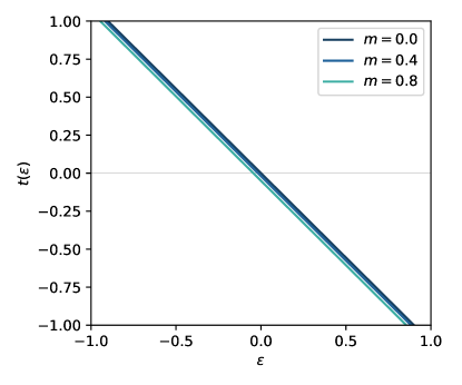
Refer to caption
Figure 6: Shift of the Hessian, from Eq. (6), as function the loss density for different values of m𝑚m. The qualitative behaviour shown in the figure does not change varying the parameter of the systems, i.e. it is always a decreasing function. The figure shows results obtained using p=3𝑝3p=3, Δp=1.0subscriptΔ𝑝1.0\Delta_{p}=1.0 and 1/Δ2=2.31subscriptΔ22.31/\Delta_{2}=2.3.

In the replicated Kac-Rice formula a more complicated expression appears that depends on the product of the determinants of Hessians associated to different replicas. However, using a proper reference frame, it was already noticed [34, 22] that each Hessian corresponds also to a GOE since it is dominated by a (Nn)×(Nn)𝑁𝑛𝑁𝑛(N-n)\times(N-n) GOE block as nNmuch-less-than𝑛𝑁n\ll N. Moreover it has also been shown [34, 22] that the expectation value of the product the Hessian determinants is equivalent to the product of the expectation values of each determinant. Thus we can still use standard results on the spectrum of GOE random matrices to evaluate the term in the Kac-Rice that depends on the Hessian. The distribution of the spectrum of the eigenvalue is given by

ρ(λ)dλ=4Q′′(1)(λ+γ)22πQ′′(1)dλ,𝜌𝜆𝑑𝜆4superscript𝑄′′1superscript𝜆𝛾22𝜋superscript𝑄′′1𝑑𝜆\rho(\lambda)d\lambda=\frac{\sqrt{4Q^{\prime\prime}(1)-(\lambda+\gamma)^{2}}}{2\pi Q^{\prime\prime}(1)}d\lambda\,, (41)

thus the determinant is given by

ρ(λ)log|λ|dλ=12log[2Q′′(1)]+1π2λ2log|λγ/Q′′(1)|dλ.𝜌𝜆𝜆𝑑𝜆122superscript𝑄′′11𝜋2superscript𝜆2𝜆𝛾superscript𝑄′′1𝑑𝜆\int\rho(\lambda)\log|\lambda|\,d\lambda=\frac{1}{2}\log[2Q^{\prime\prime}(1)]+\frac{1}{\pi}\int\sqrt{2-\lambda^{2}}\log\left|\lambda-\gamma/\sqrt{Q^{\prime\prime}(1)}\right|d\lambda\,. (42)

where we recognise t=γ/Q′′(1)𝑡𝛾superscript𝑄′′1t=\gamma/\sqrt{Q^{\prime\prime}(1)}. After some algebra we find:

12log[Q′′(1)]12+Φ(t)12superscript𝑄′′112Φ𝑡\frac{1}{2}\log[Q^{\prime\prime}(1)]-\frac{1}{2}+\Phi(t) (43)

with Φ(t)Φ𝑡\Phi(t) defined in Eq. (18).

A.2.3 Complexities: Putting pieces together

By putting the above pieces together we obtain the annealed complexity of stationary points Eq. (17) where we can finally distinguish the origin of the various terms: the first term comes from the normalisation of the density and the determinant of the Hessian, the second comes from the volume prefactor, the third, fourth and fifth terms are originated by the probability density of loss and gradient and the last term comes from the product of Hessians.

In order to select only the minima in the study of the complexity we must impose that the smallest eigenvalue is positive. There are two possible scenarios: either the smallest eigenvalue is determined by the left edge of the bulk of the spectrum (the perturbation does not induces any BBP transition), or it is outside the bulk of the spectrum. In the first case the probability that the smallest eigenvalue is positive is suppressed by a factor eN2superscript𝑒superscript𝑁2e^{-N^{2}} and the corresponding large deviation function is infinite. In the second case the large deviation function associated to the shift in the position of the smallest eigenvalue, that would allow to keep it positive, is finite and must be evaluated. The problem can be addressed with a replica computation [22] and focuses only on the typical value of the eigenvalue, missing the large deviation function. As we already discussed as m0𝑚0m\rightarrow 0 we found numerically that the overlap q𝑞q that extremises the complexity is q=0𝑞0q=0, which leads back to the annealed complexity as we have shown computing the density. Since the main focus in the paper is on the critical points at the equator we do not compute the isolated eigenvalue in a quenched approach but we rather use the large deviation function as it can be obtained in the annealed approximation [37] of which we report here the result. The condition on having a positive minimum eigenvalue suppresses the number of critical points by a factor eNL(θ,t)superscript𝑒𝑁𝐿𝜃𝑡e^{-NL(\theta,t)}, with L(θ,t)𝐿𝜃𝑡L(\theta,t) given in Eq. (20), that enters in Eq. (17) leading to Eq. (19).

Remark 2 (threshold loss)

Considering Eq. (17) and changing variables from (ϵp,ϵ2)subscriptitalic-ϵ𝑝subscriptitalic-ϵ2(\epsilon_{p},\epsilon_{2}) to (ϵ,t)italic-ϵ𝑡(\epsilon,t) in the maximisation. We can now specialise on the region with no overlap with the signal, m=0𝑚0m=0, and consider that the Hessian of the loss touches the zero, t=2𝑡2t=2 which simplifies the expression of the piecewise term Φ(t)Φ𝑡\Phi(t). The result is a quadratic equation in t𝑡t which is equal to 222 because of the marginality condition and can be solved in the energy ϵitalic-ϵ\epsilon. The resulting energy is the Kac-Rice threshold energy,

ϵthKR=1Q′′(1)Q(1)[(p2)22pΔ2Δp2Q′′(1)Q(1)].superscriptsubscriptitalic-ϵthKR1superscript𝑄′′1superscript𝑄1delimited-[]superscript𝑝222𝑝subscriptΔ2subscriptΔ𝑝2superscript𝑄′′1𝑄1\epsilon_{\text{\rm th}}^{\text{\rm KR}}=\frac{1}{\sqrt{Q^{\prime\prime}(1)}Q^{\prime}(1)}\left[\frac{(p-2)^{2}}{2p\Delta_{2}\Delta_{p}}-2Q^{\prime\prime}(1)Q(1)\right]\,. (44)

Appendix B CHSCK Equations

In this section we present a derivation of CHSCK equations for the spiked matrix-tensor model using the generating functional formalism and later the asymptotic analysis under the hypothesis presented in the main text. The starting point is the loss, Eq. (3), expliciting the observations, Eqs. (1-2),

(𝝈|𝑻,𝒀)=(p1)!ΔpNi1<<ipηi1ipσi1σip1pΔp𝝈,𝝈p+1Δ2Ni<jηijσiσj12Δ2𝝈,𝝈2\begin{split}\text{\large$\ell$}(\boldsymbol{\sigma}|\boldsymbol{T},\boldsymbol{Y})&=-\frac{\sqrt{(p-1)!}}{\Delta_{p}\sqrt{N}}\sum_{i_{1}<\dots<i_{p}}\eta_{i_{1}\dots i_{p}}\sigma_{i_{1}}\dots\sigma_{i_{p}}-\frac{1}{p\Delta_{p}}\langle\boldsymbol{\sigma},\boldsymbol{\sigma}^{*}\rangle^{p}+\\ &-\frac{1}{\Delta_{2}\sqrt{N}}\sum_{i<j}\eta_{ij}\sigma_{i}\sigma_{j}-\frac{1}{2\Delta_{2}}\langle\boldsymbol{\sigma},\boldsymbol{\sigma}^{*}\rangle^{2}\end{split} (45)

and the gradient flow Eq. (4) that for mathematical convenience we associate to an auxiliary function 𝒇(𝝈)𝒇𝝈\boldsymbol{f}(\boldsymbol{\sigma})

σ˙i(t)=μ(t)σ(t)(𝝈(t)|𝑻,𝒀)σi(t)fi(𝝈(t)).subscript˙𝜎𝑖𝑡𝜇𝑡𝜎𝑡conditional𝝈𝑡𝑻𝒀subscript𝜎𝑖𝑡approaches-limitsubscript𝑓𝑖𝝈𝑡\dot{\sigma}_{i}(t)=-\mu(t)\sigma(t)-\frac{\partial\text{\large$\ell$}(\boldsymbol{\sigma}(t)|\boldsymbol{T},\boldsymbol{Y})}{\partial\sigma_{i}(t)}\doteq f_{i}\left(\boldsymbol{\sigma}(t)\right)\,. (46)

The next section shows in detail the derivation that proceeds by introducing a probability distribution for the different evolutions, or trajectories, of the dynamics at a fixed realization of the noise. Then the distribution is averaged over the noise and this implies some technical steps before obtaining the final form. The resulting distribution is used to average correlation, response function and magnetisation over all the trajectories giving the CHSCK Eqs. (8-11). In the analysis an important role is played by the normalisation constant of the distribution of the trajectories, that is used in the final steps to derive with simplicity the equations.

After deriving the equations we show how to apply the hypothesis on the large time behaviour of t𝑡t and tsuperscript𝑡t^{\prime} to the CHSCK Eqs. In the last part this analysis provides the constants R¯¯𝑅\overline{R} and μsubscript𝜇\mu_{\infty} used to the derive the threshold in the main text, and some interesting additional information, such as the value of the loss at the threshold shown in the right panel of Fig. 4.

B.1 Derivation of CHSCK Equations

The first step is to discretise the time in M𝑀M time steps of length hh. We want the trajectories to be a solution at every time step of Eq. (4), which discretized looks as σia+1σia=fi(𝝈a)hsuperscriptsubscript𝜎𝑖𝑎1superscriptsubscript𝜎𝑖𝑎subscript𝑓𝑖superscript𝝈𝑎\sigma_{i}^{a+1}-\sigma_{i}^{a}=f_{i}\left(\boldsymbol{\sigma}^{a}\right)h with a𝑎a the time index. Let’s call ya+1superscript𝑦𝑎1y^{a+1} a solution to this equation. We can define the probability density of observing a trajectory satisfying Eq. (4) at a fixed noise:

p(𝝈1,,𝝈M)=aiδ(σia+1yia(𝝈a))a=0M1dμ𝕊a.𝑝superscript𝝈1superscript𝝈𝑀subscriptproduct𝑎𝑖𝛿superscriptsubscript𝜎𝑖𝑎1superscriptsubscript𝑦𝑖𝑎superscript𝝈𝑎superscriptsubscriptproduct𝑎0𝑀1𝑑superscriptsubscript𝜇𝕊𝑎p(\boldsymbol{\sigma}^{1},\dots,\boldsymbol{\sigma}^{M})=\int\prod_{ai}\delta\left(\sigma_{i}^{a+1}-y_{i}^{a}(\boldsymbol{\sigma}^{a})\right)\prod_{a=0}^{M-1}d\mu_{\mathbb{S}}^{a}\,. (47)

where μ𝕊subscript𝜇𝕊\mu_{\mathbb{S}} is the measure over 𝕊N1superscript𝕊𝑁1\mathbb{S}^{N-1}.

The normalisation constant is the integral of this probability and is called generating functional 𝒵𝒵\mathcal{Z} and since the previous object is already properly normalised it is equal to 111. Rewriting the δ𝛿\deltas as Fourier transforms and therefore including the auxiliary variables 𝝈~asuperscript~𝝈𝑎\tilde{\boldsymbol{\sigma}}^{a},

1=aiexp[Nσ~ia(σia+1σiafi(𝝈a)h)]a=0M1dμ𝕊ad𝝈~a2πi1subscriptproduct𝑎𝑖𝑁superscriptsubscript~𝜎𝑖𝑎superscriptsubscript𝜎𝑖𝑎1superscriptsubscript𝜎𝑖𝑎subscript𝑓𝑖superscript𝝈𝑎superscriptsubscriptproduct𝑎0𝑀1𝑑superscriptsubscript𝜇𝕊𝑎𝑑superscript~𝝈𝑎2𝜋𝑖1=\int\prod_{ai}\exp\left[N\tilde{\sigma}_{i}^{a}\left(\sigma_{i}^{a+1}-\sigma_{i}^{a}-f_{i}(\boldsymbol{\sigma}^{a})h\right)\right]\prod_{a=0}^{M-1}d\mu_{\mathbb{S}}^{a}\frac{d\tilde{\boldsymbol{\sigma}}^{a}}{2\pi i} (48)

where in order to have mathematically well-defined quantities in the large N𝑁N limit we have a factor in the exponential. Moving to the continuum, the generating functional appears as a path integral

1=𝒵=𝒟[𝝈,𝝈~]iexp[Nσ~i(t)(tσi(t)fi(𝝈(t)))𝑑t].1𝒵𝒟𝝈~𝝈subscriptproduct𝑖𝑁subscript~𝜎𝑖𝑡subscript𝑡subscript𝜎𝑖𝑡subscript𝑓𝑖𝝈𝑡differential-d𝑡1=\mathcal{Z}=\int\mathcal{D}\left[\boldsymbol{\sigma},\tilde{\boldsymbol{\sigma}}\right]\prod_{i}\exp\left[N\int\tilde{\sigma}_{i}(t)\left(\partial_{t}\sigma_{i}(t)-f_{i}(\boldsymbol{\sigma}(t))\right)dt\right]\,. (49)

So far the object we derived is a distribution that tells whether a trajectory from arbitrary initial condition respects or not gradient-flow dynamics, however, our interest is in average trajectories with respect to the realization of the disorder. Therefore the distribution has to be averaged and after some algebraic manipulation gives the average generating functional in Eq. (51),

1=𝔼η[𝒵]=𝒟[𝝈,𝝈~]iexp[Nσ~i(t)(tσi(t)+μ(t)σi(t)Q(𝝈(t),𝝈p1)σi)dt]××𝔼η{iexp[σ~i(t)(N(p1)!Δpi1<<ipηii1ip1σi1σip1)dt]}××𝔼η{iexp[σ~i(t)(NΔ2jηijσj)𝑑t]}.1subscript𝔼𝜂delimited-[]𝒵𝒟𝝈~𝝈subscriptproduct𝑖𝑁subscript~𝜎𝑖𝑡subscript𝑡subscript𝜎𝑖𝑡𝜇𝑡subscript𝜎𝑖𝑡superscript𝑄superscript𝝈𝑡superscript𝝈𝑝1subscriptsuperscript𝜎𝑖𝑑𝑡subscript𝔼𝜂subscriptproduct𝑖subscript~𝜎𝑖𝑡𝑁𝑝1subscriptΔ𝑝subscriptsubscript𝑖1subscript𝑖𝑝subscript𝜂𝑖subscript𝑖1subscript𝑖𝑝1subscript𝜎subscript𝑖1subscript𝜎subscript𝑖𝑝1𝑑𝑡subscript𝔼𝜂subscriptproduct𝑖subscript~𝜎𝑖𝑡𝑁subscriptΔ2subscript𝑗subscript𝜂𝑖𝑗subscript𝜎𝑗differential-d𝑡\begin{split}1=\mathbb{E}_{\eta}&\left[\mathcal{Z}\right]=\int\mathcal{D}\left[\boldsymbol{\sigma},\tilde{\boldsymbol{\sigma}}\right]\prod_{i}\exp\left[N\int\tilde{\sigma}_{i}(t)\left(\partial_{t}\sigma_{i}(t)+\mu(t)\sigma_{i}(t)-Q^{\prime}(\langle\boldsymbol{\sigma}(t),\boldsymbol{\sigma}^{*}\rangle^{p-1})\sigma^{*}_{i}\right)dt\right]\times\\ &\times\mathbb{E}_{\eta}\left\{\prod_{i}\exp\left[-\int\tilde{\sigma}_{i}(t)\left(-\frac{\sqrt{N(p-1)!}}{\Delta_{p}}\sum_{i_{1}<\dots<i_{p}}\eta_{i\,i_{1}\dots i_{p-1}}\sigma_{i_{1}}\dots\sigma_{i_{p-1}}\right)dt\right]\right\}\times\\ &\times\mathbb{E}_{\eta}\left\{\prod_{i}\exp\left[-\int\tilde{\sigma}_{i}(t)\left(-\frac{\sqrt{N}}{\Delta_{2}}\sum_{j}\eta_{ij}\sigma_{j}\right)dt\right]\right\}\,.\end{split} (50)

In averaging over the η𝜂\eta we need to be careful in grouping all the permutations of i𝑖i with i1,,ip1subscript𝑖1subscript𝑖𝑝1i_{1},\dots,i_{p-1}. For instance the exponent of the term in p𝑝p is gives by

N(p1)!Δpi1<<ipηi1ip(σ~i1(t)σi2(t)σip(t)++σi1(t)σi2(t)σ~ip(t))𝑑t=N(p1)!2Δpi1<<ip(σ~i1(t)σi2(t)σip(t)+perm.)(σ~i1(t)σi2(t)σip(t)+perm.)𝑑t𝑑t=N2Δp(𝝈~(t),𝝈~(t)𝝈(t),𝝈(t)p1+(p1)𝝈~(t),𝝈(t)𝝈(t),𝝈~(t)𝝈(t),𝝈(t)p2)𝑑t𝑑t.𝑁𝑝1subscriptΔ𝑝subscriptsubscript𝑖1subscript𝑖𝑝subscript𝜂subscript𝑖1subscript𝑖𝑝subscript~𝜎subscript𝑖1𝑡subscript𝜎subscript𝑖2𝑡subscript𝜎subscript𝑖𝑝𝑡subscript𝜎subscript𝑖1𝑡subscript𝜎subscript𝑖2𝑡subscript~𝜎subscript𝑖𝑝𝑡differential-d𝑡𝑁𝑝12subscriptΔ𝑝subscriptsubscript𝑖1subscript𝑖𝑝double-integralsubscript~𝜎subscript𝑖1𝑡subscript𝜎subscript𝑖2𝑡subscript𝜎subscript𝑖𝑝𝑡perm.subscript~𝜎subscript𝑖1superscript𝑡subscript𝜎subscript𝑖2superscript𝑡subscript𝜎subscript𝑖𝑝superscript𝑡perm.differential-d𝑡differential-dsuperscript𝑡𝑁2subscriptΔ𝑝double-integral~𝝈𝑡~𝝈superscript𝑡superscript𝝈𝑡𝝈𝑡𝑝1𝑝1~𝝈𝑡𝝈superscript𝑡𝝈𝑡~𝝈superscript𝑡superscript𝝈𝑡𝝈𝑡𝑝2differential-d𝑡differential-dsuperscript𝑡\begin{split}&-\frac{\sqrt{N(p-1)!}}{\Delta_{p}}\!\!\!\sum_{i_{1}<\dots<i_{p}}\int\eta_{i_{1}\dots i_{p}}\left(\tilde{\sigma}_{i_{1}}(t)\sigma_{i_{2}}(t)\dots\sigma_{i_{p}}(t)+\dots+\sigma_{i_{1}}(t)\sigma_{i_{2}}(t)\dots\tilde{\sigma}_{i_{p}}(t)\right)dt\\ &\,=\frac{N(p-1)!}{2\Delta_{p}}\!\!\!\sum_{i_{1}<\dots<i_{p}}\!\!\iint\!\left(\tilde{\sigma}_{i_{1}}(t)\sigma_{i_{2}}(t)\dots\sigma_{i_{p}}(t)\!+\!\text{perm.}\right)\!\left(\tilde{\sigma}_{i_{1}}(t^{\prime})\sigma_{i_{2}}(t^{\prime})\dots\sigma_{i_{p}}(t^{\prime})\!+\!\text{perm.}\right)dtdt^{\prime}\\ &\,=\frac{N}{2\Delta_{p}}\!\!\iint\!\left(\langle\tilde{\boldsymbol{\sigma}}(t),\tilde{\boldsymbol{\sigma}}(t^{\prime})\rangle\langle\boldsymbol{\sigma}(t),\boldsymbol{\sigma}(t)\rangle^{p-1}\!\!+\!(p-1)\langle\tilde{\boldsymbol{\sigma}}(t),\boldsymbol{\sigma}(t^{\prime})\rangle\langle\boldsymbol{\sigma}(t),\tilde{\boldsymbol{\sigma}}(t^{\prime})\rangle\langle\boldsymbol{\sigma}(t),\boldsymbol{\sigma}(t)\rangle^{p-2}\right)dtdt^{\prime}.\end{split}

This gives an action 𝒮[𝝈,𝝈~]𝒮𝝈~𝝈\mathcal{S}[\boldsymbol{\sigma},\tilde{\boldsymbol{\sigma}}] defined by

1=𝒵¯=𝒟[𝝈,𝝈~]e𝒮[𝝈,𝝈~]==𝒟[𝝈,𝝈~]iexp[Nσ~i(t)(tσi(t)+μ(t)σi(t)Q(𝝈(t),𝝈p1)σi)dt]××exp[N2Δp𝝈~(t),𝝈~(t)𝝈(t),𝝈(t)p1dtdt]××exp[N2Δp(p1)𝝈~(t),𝝈(t)𝝈(t),𝝈~(t)𝝈(t),𝝈(t)p2dtdt]××exp[N2Δ2(𝝈~(t),𝝈~(t)𝝈(t),𝝈(t)+𝝈~(t),𝝈(t)𝝈(t),𝝈~(t))𝑑t𝑑t].1¯𝒵𝒟𝝈~𝝈superscript𝑒𝒮𝝈~𝝈𝒟𝝈~𝝈subscriptproduct𝑖𝑁subscript~𝜎𝑖𝑡subscript𝑡subscript𝜎𝑖𝑡𝜇𝑡subscript𝜎𝑖𝑡superscript𝑄superscript𝝈𝑡superscript𝝈𝑝1subscriptsuperscript𝜎𝑖𝑑𝑡𝑁2subscriptΔ𝑝double-integral~𝝈𝑡~𝝈superscript𝑡superscript𝝈𝑡𝝈𝑡𝑝1𝑑𝑡𝑑superscript𝑡𝑁2subscriptΔ𝑝double-integral𝑝1~𝝈𝑡𝝈superscript𝑡𝝈𝑡~𝝈superscript𝑡superscript𝝈𝑡𝝈𝑡𝑝2𝑑𝑡𝑑superscript𝑡𝑁2subscriptΔ2double-integral~𝝈𝑡~𝝈superscript𝑡𝝈𝑡𝝈𝑡~𝝈𝑡𝝈superscript𝑡𝝈𝑡~𝝈superscript𝑡differential-d𝑡differential-dsuperscript𝑡\begin{split}1&=\overline{\mathcal{Z}}=\int\mathcal{D}[\boldsymbol{\sigma},\tilde{\boldsymbol{\sigma}}]e^{\mathcal{S}[\boldsymbol{\sigma},\tilde{\boldsymbol{\sigma}}]}=\\ &=\int\mathcal{D}\left[\boldsymbol{\sigma},\tilde{\boldsymbol{\sigma}}\right]\prod_{i}\exp\left[N\int\tilde{\sigma}_{i}(t)\left(\partial_{t}\sigma_{i}(t)+\mu(t)\sigma_{i}(t)-Q^{\prime}(\langle\boldsymbol{\sigma}(t),\boldsymbol{\sigma}^{*}\rangle^{p-1})\sigma^{*}_{i}\right)dt\right]\times\\ &\times\exp\left[\frac{N}{2\Delta_{p}}\iint\langle\tilde{\boldsymbol{\sigma}}(t),\tilde{\boldsymbol{\sigma}}(t^{\prime})\rangle\langle\boldsymbol{\sigma}(t),\boldsymbol{\sigma}(t)\rangle^{p-1}dtdt^{\prime}\right]\times\\ &\times\exp\left[\frac{N}{2\Delta_{p}}\iint(p-1)\langle\tilde{\boldsymbol{\sigma}}(t),\boldsymbol{\sigma}(t^{\prime})\rangle\langle\boldsymbol{\sigma}(t),\tilde{\boldsymbol{\sigma}}(t^{\prime})\rangle\langle\boldsymbol{\sigma}(t),\boldsymbol{\sigma}(t)\rangle^{p-2}dtdt^{\prime}\right]\times\\ &\times\exp\left[\frac{N}{2\Delta_{2}}\iint\left(\langle\tilde{\boldsymbol{\sigma}}(t),\tilde{\boldsymbol{\sigma}}(t^{\prime})\rangle\langle\boldsymbol{\sigma}(t),\boldsymbol{\sigma}(t)\rangle+\langle\tilde{\boldsymbol{\sigma}}(t),\boldsymbol{\sigma}(t^{\prime})\rangle\langle\boldsymbol{\sigma}(t),\tilde{\boldsymbol{\sigma}}(t^{\prime})\rangle\right)dtdt^{\prime}\right]\,.\end{split} (51)

A simple way to proceed once evaluated the action was proposed in [38] and consists in taking the expectation with respect to the path distribution and exploiting simple identities together with integration by part:

0=δσi(t)δσ~i(t)𝒮=σi(t)δ𝒮δσ~i(t)𝒮==Ntσi(t)σi(t)+μ(t)σi(t)σi(t)Q(𝝈(t),𝝈p1)σiσi(t)++1Δp[𝝈(t),𝝈(t)p1σ~i(t′′)+(p1)𝝈~(t),𝝈(t′′)𝝈(t),𝝈(t)p2σi(t′′)]𝑑t′′++1Δ2[𝝈(t),𝝈(t)σ~i(t′′)+𝝈~(t),𝝈(t′′)σi(t′′)]dt′′𝒮.0subscriptdelimited-⟨⟩𝛿subscript𝜎𝑖superscript𝑡𝛿subscript~𝜎𝑖𝑡𝒮subscriptdelimited-⟨⟩subscript𝜎𝑖superscript𝑡𝛿𝒮𝛿subscript~𝜎𝑖𝑡𝒮𝑁subscriptdelimited-⟨⟩subscript𝑡subscript𝜎𝑖𝑡subscript𝜎𝑖superscript𝑡𝜇𝑡subscript𝜎𝑖𝑡subscript𝜎𝑖superscript𝑡superscript𝑄superscript𝝈𝑡superscript𝝈𝑝1subscriptsuperscript𝜎𝑖subscript𝜎𝑖superscript𝑡1subscriptΔ𝑝delimited-[]superscript𝝈𝑡𝝈𝑡𝑝1subscript~𝜎𝑖superscript𝑡′′𝑝1~𝝈𝑡𝝈superscript𝑡′′superscript𝝈𝑡𝝈𝑡𝑝2subscript𝜎𝑖superscript𝑡′′differential-dsuperscript𝑡′′1subscriptΔ2delimited-[]𝝈𝑡𝝈𝑡subscript~𝜎𝑖superscript𝑡′′~𝝈𝑡𝝈superscript𝑡′′subscript𝜎𝑖superscript𝑡′′𝑑superscript𝑡′′𝒮\begin{split}0&=-\left\langle\frac{\delta\sigma_{i}(t^{\prime})}{\delta\tilde{\sigma}_{i}(t)}\right\rangle_{\mathcal{S}}=\left\langle\sigma_{i}(t^{\prime})\frac{\delta\mathcal{S}}{\delta\tilde{\sigma}_{i}(t)}\right\rangle_{\mathcal{S}}=\\ &=N\Bigg{\langle}\partial_{t}\sigma_{i}(t)\sigma_{i}(t^{\prime})+\mu(t)\sigma_{i}(t)\sigma_{i}(t^{\prime})-Q^{\prime}(\langle\boldsymbol{\sigma}(t),\boldsymbol{\sigma}^{*}\rangle^{p-1})\sigma^{*}_{i}\sigma_{i}(t^{\prime})+\\ &+\frac{1}{\Delta_{p}}\int\left[\langle\boldsymbol{\sigma}(t),\boldsymbol{\sigma}(t)\rangle^{p-1}\tilde{\sigma}_{i}(t^{\prime\prime})+(p-1)\langle\tilde{\boldsymbol{\sigma}}(t),\boldsymbol{\sigma}(t^{\prime\prime})\rangle\langle\boldsymbol{\sigma}(t),\boldsymbol{\sigma}(t)\rangle^{p-2}\sigma_{i}(t^{\prime\prime})\right]dt^{\prime\prime}+\\ &+\frac{1}{\Delta_{2}}\int\left[\langle\boldsymbol{\sigma}(t),\boldsymbol{\sigma}(t)\rangle\tilde{\sigma}_{i}(t^{\prime\prime})+\langle\tilde{\boldsymbol{\sigma}}(t),\boldsymbol{\sigma}(t^{\prime\prime})\rangle\sigma_{i}(t^{\prime\prime})\right]dt^{\prime\prime}\Bigg{\rangle}_{\mathcal{S}}\,.\end{split} (52)

Finally, summing over the index i𝑖i and dividing by N𝑁N we recover Eq. (8). The remaining CHSCK Eqs. (9-10) follow analogously from:

δ(tt)=iδσ~i(t)δσ~i(t)𝒮=iσ~i(t)δSδσ~i(t)𝒮;𝛿𝑡superscript𝑡subscript𝑖subscriptdelimited-⟨⟩𝛿subscript~𝜎𝑖superscript𝑡𝛿subscript~𝜎𝑖𝑡𝒮subscript𝑖subscriptdelimited-⟨⟩subscript~𝜎𝑖superscript𝑡𝛿𝑆𝛿subscript~𝜎𝑖𝑡𝒮\displaystyle\delta(t-t^{\prime})=\sum_{i}\left\langle\frac{\delta\tilde{\sigma}_{i}(t^{\prime})}{\delta\tilde{\sigma}_{i}(t)}\right\rangle_{\mathcal{S}}=-\sum_{i}\left\langle\tilde{\sigma}_{i}(t^{\prime})\frac{\delta S}{\delta\tilde{\sigma}_{i}(t)}\right\rangle_{\mathcal{S}}\,; (53)
0=δσiδσ~i(t)𝒮=σiδ𝒮δσ~i(t)𝒮.0subscriptdelimited-⟨⟩𝛿superscriptsubscript𝜎𝑖𝛿subscript~𝜎𝑖𝑡𝒮subscriptdelimited-⟨⟩superscriptsubscript𝜎𝑖𝛿𝒮𝛿subscript~𝜎𝑖𝑡𝒮\displaystyle 0=-\left\langle\frac{\delta\sigma_{i}^{*}}{\delta\tilde{\sigma}_{i}(t)}\right\rangle_{\mathcal{S}}=\left\langle\sigma_{i}^{*}\frac{\delta\mathcal{S}}{\delta\tilde{\sigma}_{i}(t)}\right\rangle_{\mathcal{S}}\,. (54)

and Eq. (11) comes from imposing the spherical constrain, C(t,t)=1t𝐶𝑡𝑡1for-all𝑡C(t,t)=1\quad\forall t, on Eq. (8).

In the following we are going to perform the analysis proposed by [29] in the present model. We need to consider Langevin dynamics instead of gradient-flow dynamics

σ˙i(t)=μ(t)σ(t)(𝝈(t)|𝑻,𝒀)σi(t)+1Nηi(L)(t),subscript˙𝜎𝑖𝑡𝜇𝑡𝜎𝑡conditional𝝈𝑡𝑻𝒀subscript𝜎𝑖𝑡1𝑁superscriptsubscript𝜂𝑖𝐿𝑡\dot{\sigma}_{i}(t)=-\mu(t)\sigma(t)-\frac{\partial\text{\large$\ell$}(\boldsymbol{\sigma}(t)|\boldsymbol{T},\boldsymbol{Y})}{\partial\sigma_{i}(t)}+\frac{1}{\sqrt{N}}\eta_{i}^{(L)}(t)\,, (55)

where the last term represents the Langevin noise, which is white Gaussian noise with moments: 𝔼L[ηi(L)(t)]=0subscript𝔼𝐿delimited-[]superscriptsubscript𝜂𝑖𝐿𝑡0\mathbb{E}_{L}[\eta_{i}^{(L)}(t)]=0 and 𝔼L[ηi(L)(t)ηj(L)(t)]=2Tδijδ(tt)subscript𝔼𝐿delimited-[]superscriptsubscript𝜂𝑖𝐿𝑡superscriptsubscript𝜂𝑗𝐿superscript𝑡2𝑇subscript𝛿𝑖𝑗𝛿𝑡superscript𝑡\mathbb{E}_{L}[\eta_{i}^{(L)}(t)\eta_{j}^{(L)}(t^{\prime})]=2T\delta_{ij}\delta(t-t^{\prime}) with T𝑇T that has the physical meaning of temperature. The CHSCK equations are slightly modified,

tC(t,t)=TR(t,t)μ(t)C(t,t)+Q(m(t))m(t)++0tR(t,t′′)Q′′(C(t,t′′))C(t,t′′)𝑑t′′+0tR(t,t′′)Q(C(t,t′′))𝑑t′′,𝑡𝐶𝑡superscript𝑡𝑇𝑅superscript𝑡𝑡𝜇𝑡𝐶𝑡superscript𝑡superscript𝑄𝑚𝑡𝑚superscript𝑡superscriptsubscript0𝑡𝑅𝑡superscript𝑡′′superscript𝑄′′𝐶𝑡superscript𝑡′′𝐶superscript𝑡superscript𝑡′′differential-dsuperscript𝑡′′superscriptsubscript0superscript𝑡𝑅superscript𝑡superscript𝑡′′superscript𝑄𝐶𝑡superscript𝑡′′differential-dsuperscript𝑡′′\displaystyle\begin{split}&\frac{\partial}{\partial t}C(t,t^{\prime})=TR(t^{\prime},t)-\mu(t)\,C(t,t^{\prime})+Q^{\prime}(m(t))m(t^{\prime})+\\ &\quad+\int_{0}^{t}R(t,t^{\prime\prime})Q^{\prime\prime}(C(t,t^{\prime\prime}))C(t^{\prime},t^{\prime\prime})dt^{\prime\prime}+\int_{0}^{t^{\prime}}R(t^{\prime},t^{\prime\prime})Q^{\prime}(C(t,t^{\prime\prime}))dt^{\prime\prime}\,,\end{split} (56)
tR(t,t)=μ(t)R(t,t)+ttR(t,t′′)Q′′(C(t,t′′))R(t′′,t)𝑑t′′,𝑡𝑅𝑡superscript𝑡𝜇𝑡𝑅𝑡superscript𝑡superscriptsubscriptsuperscript𝑡𝑡𝑅𝑡superscript𝑡′′superscript𝑄′′𝐶𝑡superscript𝑡′′𝑅superscript𝑡′′superscript𝑡differential-dsuperscript𝑡′′\displaystyle\begin{split}&\frac{\partial}{\partial t}R(t,t^{\prime})=-\mu(t)\,R(t,t^{\prime})+\int_{t^{\prime}}^{t}R(t,t^{\prime\prime})Q^{\prime\prime}(C(t,t^{\prime\prime}))R(t^{\prime\prime},t^{\prime})dt^{\prime\prime}\,,\end{split} (57)
tm(t)=μ(t)m(t)+Q(m(t))+0tR(t,t′′)m(t′′)Q′′(C(t,t′′))𝑑t′′,𝑡𝑚𝑡𝜇𝑡𝑚𝑡superscript𝑄𝑚𝑡superscriptsubscript0𝑡𝑅𝑡superscript𝑡′′𝑚superscript𝑡′′superscript𝑄′′𝐶𝑡superscript𝑡′′differential-dsuperscript𝑡′′\displaystyle\begin{split}&\frac{\partial}{\partial t}m(t)=-\mu(t)\,m(t)+Q^{\prime}(m(t))+\int_{0}^{t}R(t,t^{\prime\prime})m(t^{\prime\prime})Q^{\prime\prime}(C(t,t^{\prime\prime}))dt^{\prime\prime}\,,\end{split} (58)
μ(t)=T+Q(m(t))m(t)+0tR(t,t′′)[Q(C(t,t′′))+Q′′(C(t,t′′))C(t,t′′)]𝑑t′′.𝜇𝑡𝑇superscript𝑄𝑚𝑡𝑚𝑡superscriptsubscript0𝑡𝑅𝑡superscript𝑡′′delimited-[]superscript𝑄𝐶𝑡superscript𝑡′′superscript𝑄′′𝐶𝑡superscript𝑡′′𝐶𝑡superscript𝑡′′differential-dsuperscript𝑡′′\displaystyle\begin{split}&\mu(t)=T+Q^{\prime}(m(t))m(t)+\int_{0}^{t}R(t,t^{\prime\prime})\left[Q^{\prime}(C(t,t^{\prime\prime}))+Q^{\prime\prime}(C(t,t^{\prime\prime}))C(t,t^{\prime\prime})\right]dt^{\prime\prime}\,.\end{split} (59)

B.2 CHSCK Equations Separation of Time-Scales
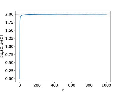
Refer to caption
Figure 7: t=(pϵp(t)+2ϵ2(t))/Q′′(1)𝑡𝑝subscriptitalic-ϵ𝑝𝑡2subscriptitalic-ϵ2𝑡superscript𝑄′′1t=-\left(p\epsilon_{p}(t)+2\epsilon_{2}(t)\right)/\sqrt{Q^{\prime\prime}(1)} for p=3𝑝3p=3, Δp=1.0subscriptΔ𝑝1.0\Delta_{p}=1.0 and 1/Δ2=1.91subscriptΔ21.91/\Delta_{2}=1.9 evaluated numerically from the CHSCK equations.
Refer to caption
Figure 8: Support of the density of eigenvalues of the Hessian along the dynamics for p=3𝑝3p=3, Δp=1.0subscriptΔ𝑝1.0\Delta_{p}=1.0 and 1/Δ2=1.91subscriptΔ21.91/\Delta_{2}=1.9. This figure illustrates the GF tends to the marginally stable minima for low signal-to-noise ratio.
Refer to caption
Figure 9: The correlation function C(t,t)𝐶𝑡superscript𝑡C(t,t^{\prime}) with p=3𝑝3p=3, Δp=1.0subscriptΔ𝑝1.0\Delta_{p}=1.0 and 1/Δ2=1.51subscriptΔ21.51/\Delta_{2}=1.5 evaluated numerically from the CHSCK equations. The correlation is plotted as difference of the two times showing the as ttt,tmuch-less-than𝑡superscript𝑡𝑡superscript𝑡t-t^{\prime}\ll t,t^{\prime} it remains close to 111. This shows as well that in this regime the correlation function shows time translational invariance.

The theory of glassy dynamics [25] is quite involved. We have therefore decided to show first some numerical results that directly confirm assumptions made in the main text, and then show in full glory that these assumptions can be obtained analytically from the theory.

B.2.1 Numerical tests

The first property that we wish to test is that for low signal-to-noise ratio GF is trapped in minima that are marginally stable. This can be checked computing from the CHSCK equations the evolution of t=(pϵp(t)+2ϵ2(t))/Q′′(1)𝑡𝑝subscriptitalic-ϵ𝑝𝑡2subscriptitalic-ϵ2𝑡superscript𝑄′′1t=-\left(p\epsilon_{p}(t)+2\epsilon_{2}(t)\right)/\sqrt{Q^{\prime\prime}(1)}, the terms ϵp(t)subscriptitalic-ϵ𝑝𝑡\epsilon_{p}(t) and ϵ2(t)subscriptitalic-ϵ2𝑡\epsilon_{2}(t) can be expressed in terms of C,R,m𝐶𝑅𝑚C,R,m as shown in Rmk. 6 of section B.2.6. In Fig. 7 we show that t=(pϵp(t)+2ϵ2(t))/Q′′(1)𝑡𝑝subscriptitalic-ϵ𝑝𝑡2subscriptitalic-ϵ2𝑡superscript𝑄′′1t=-\left(p\epsilon_{p}(t)+2\epsilon_{2}(t)\right)/\sqrt{Q^{\prime\prime}(1)} (ϵp(t)subscriptitalic-ϵ𝑝𝑡\epsilon_{p}(t) starts from zero at initial time and then converges to two. Thus the minima to which GF tends to at long times and for small signal-to-noise ratio are indeed the marginally stable ones characterized by a spectrum of the Hessian whose left edge touches zero. Actually, transferring the results obtained in the context of spin-glasses to our case [39], we know that as long as m𝑚m remains zero, i.e for small signal-to-noise ratio, the spectrum of the Hessian along the dynamics is a Wigner semi-circle with support [Q′′(1)(2+t),Q′′(1)(2+t)]superscript𝑄′′12𝑡superscript𝑄′′12𝑡[\sqrt{Q^{\prime\prime}(1)}(-2+t),\sqrt{Q^{\prime\prime}(1)}(2+t)]. We show the evolution of the support as a function of time in Fig. 8. This is another illustration of the fact that minima trapping GF are marginally stable.

The other point we wish to test is the assumption (i) made in the main text on C(t,t)𝐶𝑡superscript𝑡C(t,t^{\prime}), which we repeat here for convenience: C(t,t)=1𝐶𝑡superscript𝑡1C(t,t^{\prime})=1 when tt𝑡superscript𝑡t-t^{\prime} finite; C(t,t)𝐶𝑡superscript𝑡C(t,t^{\prime}) becomes less than one when tt𝑡superscript𝑡t-t^{\prime} diverges with t𝑡t and tsuperscript𝑡t^{\prime}. We show in Fig. 9 the correlation function C(t,t)𝐶𝑡superscript𝑡C(t,t^{\prime}) as a function of tt𝑡superscript𝑡t-t^{\prime} (in log-scale) for several values of tsuperscript𝑡t^{\prime}. This is a good illustration of the "aging ansatz" defined in the main text.

Let us stress that these numerical tests where already done in the past on similar spin-glass models. We show them here in order to make the paper self-contained and so that the reader does not have to go back to physics literature. In the same vein, in the next sections we show the full theoretical analysis of the dynamical equations, which closely follows the theory of glassy dynamics developed in physics [25].

B.2.2 General aging ansatz

We study the behaviours of the dynamics at large times in the two-time regimes introduced in the main text (now generalized at finite temperature).

  1. 1.

    t,t1much-greater-than𝑡superscript𝑡1t,t^{\prime}\gg 1 with ttt0𝑡superscript𝑡𝑡0\frac{t-t^{\prime}}{t}\rightarrow 0, see Fig. 9. In this regime we have two important aspects: the two-times function depends only on the difference of the two times, τ=tt𝜏𝑡superscript𝑡\tau=t-t^{\prime}, and we say that they respect time-translational invariance. Under this observation we redefine the two functions as C(t,t)CTTI(τ)C(tt,0)𝐶𝑡superscript𝑡subscript𝐶TTI𝜏𝐶𝑡superscript𝑡0C(t,t^{\prime})\rightarrow C_{\text{TTI}}(\tau)\equiv C(t-t^{\prime},0) and R(t,t)RTTI(τ)R(tt,0)𝑅𝑡superscript𝑡subscript𝑅TTI𝜏𝑅𝑡superscript𝑡0R(t,t^{\prime})\rightarrow R_{\text{TTI}}(\tau)\equiv R(t-t^{\prime},0). The second important aspect is the validity of the fluctuation-dissipation theorem (FDT) that links correlation and response function by the relation RTTI(τ)=1TdCTTIdτ(τ)subscript𝑅TTI𝜏1𝑇𝑑subscript𝐶TTI𝑑𝜏𝜏R_{\text{TTI}}(\tau)=-\frac{1}{T}\frac{dC_{\text{TTI}}}{d\tau}(\tau) for τ𝜏\tau positive.

  2. 2.

    t,t1much-greater-than𝑡superscript𝑡1t,t^{\prime}\gg 1 with ttt=O(1)𝑡superscript𝑡𝑡𝑂1\frac{t-t^{\prime}}{t}=O(1). In this regime the relevant variable to consider is λ=tt𝜆superscript𝑡𝑡\lambda=\frac{t^{\prime}}{t}. In reason of the "weak-long term memory" property it is useful to redefine rescale the response function and define (λ)=tR(t,t)𝜆𝑡𝑅𝑡superscript𝑡\mathcal{R}(\lambda)=tR(t,t^{\prime}). It is also convenient to consider the function q𝒞(λ)=C(t,t)𝑞𝒞𝜆𝐶𝑡superscript𝑡q\mathcal{C}(\lambda)=C(t,t^{\prime}) with q=limτCTTI(τ)𝑞subscript𝜏subscript𝐶TTI𝜏q=\lim_{\tau\rightarrow\infty}C_{\text{TTI}}(\tau). Finally, in this regime a generalised version of the fluctuation-dissipation theorem holds (λ)=1Txqd𝒞(λ)dλ𝜆1𝑇𝑥𝑞𝑑𝒞𝜆𝑑𝜆\mathcal{R}(\lambda)=\frac{1}{T}xq\frac{d\mathcal{C}(\lambda)}{d\lambda} where x𝑥x is called violation parameter.

Under the (generalized) FDT the equations for correlation and response function that we obtain in the two-time regime collapse into a single equation. In the first regime we analyse only the correlation because of this link, while in the second regime we consider the two equations separately since we need to determine the violation parameter x𝑥x.

In the analysis that follows we use massively the hypothesis of the two regimes to split the integrals and analyse them separately. We start analysing the single time equation for the Lagrange multiplier μ(t)𝜇𝑡\mu(t), then we proceed with the two-times function concentrating first on the time-translational invariant part and then on the aging part.

B.2.3 Langrange multiplier in the large time limit.

Starting from Eq. (59), we introduce the symbol psubscript𝑝\clubsuit_{p} to isolate the two contribution of matrix and tensor to the integral. As the time tends to infinity m𝑚m and μ𝜇\mu tend to their asymptotic value, respectively msubscript𝑚m_{\infty} and μsubscript𝜇\mu_{\infty}, Eq. (59) tends to

μ=T+Q(m)m+pp+2p=2.subscript𝜇𝑇superscript𝑄subscript𝑚subscript𝑚𝑝subscript𝑝2subscript𝑝2\mu_{\infty}=T+Q^{\prime}(m_{\infty})m_{\infty}+p\clubsuit_{p}+2\clubsuit_{p=2}\,.

We can now use the idea of the separation in two-time regimes. Call Qp(x)=xp/(pΔp)subscript𝑄𝑝𝑥superscript𝑥𝑝𝑝subscriptΔ𝑝Q_{p}(x)=x^{p}/(p\Delta_{p}) the part related to p𝑝p in Q(x)𝑄𝑥Q(x),

p=0tsubscript𝑝superscriptsubscript0𝑡\displaystyle\clubsuit_{p}=\int_{0}^{t} Qp(C(t,t′′))R(t,t′′)dt′′=FDT+aging=superscriptsubscript𝑄𝑝𝐶𝑡superscript𝑡′′𝑅𝑡superscript𝑡′′𝑑superscript𝑡′′subscriptFDTsubscriptagingabsent\displaystyle Q_{p}^{\prime}(C(t,t^{\prime\prime}))R(t,t^{\prime\prime})dt^{\prime\prime}=\int_{\text{FDT}}+\int_{\text{aging}}=
=t0Qp(C(t,tt~))R(t,tt~)𝑑t~+01(λ)Qp(q𝒞(λ))𝑑λ=absentsuperscriptsubscript𝑡0superscriptsubscript𝑄𝑝𝐶𝑡𝑡~𝑡𝑅𝑡𝑡~𝑡differential-d~𝑡superscriptsubscript01𝜆superscriptsubscript𝑄𝑝𝑞𝒞𝜆differential-d𝜆absent\displaystyle=-\int_{t}^{0}Q_{p}^{\prime}(C(t,t-\tilde{t}))R(t,t-\tilde{t})d\tilde{t}+\int_{0}^{1}\mathcal{R}(\lambda)Q_{p}^{\prime}(q\mathcal{C}(\lambda))d\lambda=
=+0Qp(CTTI(t~))RTTI(t~)𝑑t~+01(λ)Qp(q𝒞(λ))𝑑λ=absentsuperscriptsubscript0superscriptsubscript𝑄𝑝subscript𝐶TTI~𝑡subscript𝑅TTI~𝑡differential-d~𝑡superscriptsubscript01𝜆superscriptsubscript𝑄𝑝𝑞𝒞𝜆differential-d𝜆absent\displaystyle=+\int_{0}^{\infty}Q_{p}^{\prime}(C_{\text{TTI}}(\tilde{t}))R_{\text{TTI}}(\tilde{t})d\tilde{t}+\int_{0}^{1}\mathcal{R}(\lambda)Q_{p}^{\prime}(q\mathcal{C}(\lambda))d\lambda=
=01Tddt~Qp(CTTI(t~))𝑑t~+01(λ)Qp(q𝒞(λ))𝑑λ=absentsuperscriptsubscript01𝑇𝑑𝑑~𝑡subscript𝑄𝑝subscript𝐶TTI~𝑡differential-d~𝑡superscriptsubscript01𝜆superscriptsubscript𝑄𝑝𝑞𝒞𝜆differential-d𝜆absent\displaystyle=-\int_{0}^{\infty}\frac{1}{T}\frac{d}{d\tilde{t}}Q_{p}(C_{\text{TTI}}(\tilde{t}))d\tilde{t}+\int_{0}^{1}\mathcal{R}(\lambda)Q_{p}^{\prime}(q\mathcal{C}(\lambda))d\lambda=
=1qpTΔp+01(λ)Qp(q𝒞(λ))𝑑λabsent1superscript𝑞𝑝𝑇subscriptΔ𝑝superscriptsubscript01𝜆superscriptsubscript𝑄𝑝𝑞𝒞𝜆differential-d𝜆\displaystyle=\frac{1-q^{p}}{T\Delta_{p}}+\int_{0}^{1}\mathcal{R}(\lambda)Q_{p}^{\prime}(q\mathcal{C}(\lambda))d\lambda\,

the resulting equation is

μ=T+Q(m)m+1T[Q(1)qQ(q)]++p01(λ)Qp(q𝒞(λ))𝑑λ+201(λ)Q2(q𝒞(λ))𝑑λ.subscript𝜇𝑇superscript𝑄subscript𝑚subscript𝑚1𝑇delimited-[]superscript𝑄1𝑞superscript𝑄𝑞𝑝superscriptsubscript01𝜆superscriptsubscript𝑄𝑝𝑞𝒞𝜆differential-d𝜆2superscriptsubscript01𝜆superscriptsubscript𝑄2𝑞𝒞𝜆differential-d𝜆\begin{split}\mu_{\infty}&=T+Q^{\prime}(m_{\infty})m_{\infty}+\frac{1}{T}\left[Q^{\prime}(1)-q\,Q^{\prime}(q)\right]+\\ &+p\int_{0}^{1}\mathcal{R}(\lambda)Q_{p}^{\prime}(q\mathcal{C}(\lambda))d\lambda+2\int_{0}^{1}\mathcal{R}(\lambda)Q_{2}^{\prime}(q\mathcal{C}(\lambda))d\lambda\,.\end{split} (60)

B.2.4 Regime 1: FDT.

We apply the same scheme of separating the times scale and applying FDT to the correlation function. All over the analysis we isolate terms in the equations using the symbols \clubsuit and \spadesuit. Eq. (56) in the large time is

(τ+μ)CTTI(τ)=Q(m)m++,subscript𝜏subscript𝜇subscript𝐶TTI𝜏superscript𝑄subscript𝑚subscript𝑚(\partial_{\tau}+\mu_{\infty})C_{\text{TTI}}(\tau)=Q^{\prime}(m_{\infty})m_{\infty}+\spadesuit+\clubsuit\,, (61)

with:

\displaystyle\clubsuit =0tQ(C(t,t′′))R(t,t′′)𝑑t′′=FDT+aging=absentsuperscriptsubscript0superscript𝑡superscript𝑄𝐶𝑡superscript𝑡′′𝑅superscript𝑡superscript𝑡′′differential-dsuperscript𝑡′′subscriptFDTsubscriptagingabsent\displaystyle=\int_{0}^{t^{\prime}}Q^{\prime}(C(t,t^{\prime\prime}))R(t^{\prime},t^{\prime\prime})dt^{\prime\prime}=\int_{\text{FDT}}+\int_{\text{aging}}=
=t0Q(C(t,tt~))R(t,tt~)𝑑t~+01Q(q𝒞(λ))(λ)𝑑λ=absentsuperscriptsubscriptsuperscript𝑡0superscript𝑄𝐶𝑡superscript𝑡~𝑡𝑅superscript𝑡superscript𝑡~𝑡differential-d~𝑡superscriptsubscript01superscript𝑄𝑞𝒞𝜆𝜆differential-d𝜆absent\displaystyle=-\int_{t^{\prime}}^{0}Q^{\prime}(C(t,t^{\prime}-\tilde{t}))R(t^{\prime},t^{\prime}-\tilde{t})d\tilde{t}+\int_{0}^{1}Q^{\prime}(q\mathcal{C}(\lambda))\mathcal{R}(\lambda)d\lambda=
=1T0Q(CTTI(τ+t~))ddt~CTTI(t~)𝑑t~+01Q(q𝒞(λ))(λ)𝑑λabsent1𝑇superscriptsubscript0superscript𝑄subscript𝐶TTI𝜏~𝑡𝑑𝑑~𝑡subscript𝐶TTI~𝑡differential-d~𝑡superscriptsubscript01superscript𝑄𝑞𝒞𝜆𝜆differential-d𝜆\displaystyle=-\frac{1}{T}\int_{0}^{\infty}Q^{\prime}(C_{\text{TTI}}(\tau+\tilde{t}))\frac{d}{d\tilde{t}}C_{\text{TTI}}(\tilde{t})d\tilde{t}+\int_{0}^{1}Q^{\prime}(q\mathcal{C}(\lambda))\mathcal{R}(\lambda)d\lambda

and

\displaystyle\spadesuit =0tQ′′(C(t,t′′))R(t,t′′)C(t,t′′)𝑑t′′=tt+0t=tt+FDT+aging=absentsuperscriptsubscript0𝑡superscript𝑄′′𝐶𝑡superscript𝑡′′𝑅𝑡superscript𝑡′′𝐶superscript𝑡superscript𝑡′′differential-dsuperscript𝑡′′superscriptsubscriptsuperscript𝑡𝑡superscriptsubscript0superscript𝑡superscriptsubscriptsuperscript𝑡𝑡subscriptFDTsubscriptagingabsent\displaystyle=\int_{0}^{t}Q^{\prime\prime}(C(t,t^{\prime\prime}))R(t,t^{\prime\prime})C(t^{\prime},t^{\prime\prime})dt^{\prime\prime}=\int_{t^{\prime}}^{t}+\int_{0}^{t^{\prime}}=\int_{t^{\prime}}^{t}+\int_{\text{FDT}}+\int_{\text{aging}}=
=1T[Q(1)CTTI(τ)Q(q)q]1T0τQ(CTTI(τt~))ddt~CTTI(t~)𝑑t~absent1𝑇delimited-[]superscript𝑄1subscript𝐶TTI𝜏superscript𝑄𝑞𝑞1𝑇superscriptsubscript0𝜏superscript𝑄subscript𝐶TTI𝜏~𝑡𝑑𝑑~𝑡subscript𝐶TTI~𝑡differential-d~𝑡\displaystyle=\frac{1}{T}\left[Q^{\prime}(1)C_{\text{TTI}}(\tau)-Q^{\prime}(q)q\right]-\frac{1}{T}\int_{0}^{\tau}Q^{\prime}(C_{\text{TTI}}(\tau-\tilde{t}))\frac{d}{d\tilde{t}}C_{\text{TTI}}(\tilde{t})d\tilde{t}
+1T0Q(CTTI(τ+t~))ddt~CTTI(t~)𝑑t~+01(λ)Q′′(q𝒞(λ))q𝒞(λ)𝑑λ.1𝑇superscriptsubscript0superscript𝑄subscript𝐶TTI𝜏~𝑡𝑑𝑑~𝑡subscript𝐶TTI~𝑡differential-d~𝑡superscriptsubscript01𝜆superscript𝑄′′𝑞𝒞𝜆𝑞𝒞𝜆differential-d𝜆\displaystyle+\frac{1}{T}\int_{0}^{\infty}Q^{\prime}(C_{\text{TTI}}(\tau+\tilde{t}))\frac{d}{d\tilde{t}}C_{\text{TTI}}(\tilde{t})d\tilde{t}+\int_{0}^{1}\mathcal{R}(\lambda)Q^{\prime\prime}(q\mathcal{C}(\lambda))\,q\mathcal{C}(\lambda)d\lambda\,.

Substituting these expressions and using Eq. (60) in Eq. (61) we have the first equation, which characterises the first regime

τCTTI(τ)+(1TQ(1)μ)[1CTTI(τ)]+T=1T0τQ(CTTI(ττ′′))ddτ′′CTTI(τ′′)𝑑τ′′.subscript𝜏subscript𝐶TTI𝜏1𝑇superscript𝑄1subscript𝜇delimited-[]1subscript𝐶TTI𝜏𝑇1𝑇superscriptsubscript0𝜏superscript𝑄subscript𝐶TTI𝜏superscript𝜏′′𝑑𝑑superscript𝜏′′subscript𝐶TTIsuperscript𝜏′′differential-dsuperscript𝜏′′\partial_{\tau}C_{\text{TTI}}(\tau)+\Big{(}\frac{1}{T}Q^{\prime}(1)-\mu_{\infty}\Big{)}\left[1-C_{\text{TTI}}(\tau)\right]+T=-\frac{1}{T}\int_{0}^{\tau}Q^{\prime}(C_{\text{TTI}}(\tau-\tau^{\prime\prime}))\frac{d}{d\tau^{\prime\prime}}C_{\text{TTI}}(\tau^{\prime\prime})d\tau^{\prime\prime}\,. (62)

An important limit that is used later on in the computation is when τ𝜏\tau\rightarrow\infty and the variations of CTTIsubscript𝐶TTIC_{\text{TTI}} becomes irrelevant. This gives:

μ=T1q+Q(1)Q(q)T.subscript𝜇𝑇1𝑞superscript𝑄1superscript𝑄𝑞𝑇\mu_{\infty}=\frac{T}{1-q}+\frac{Q^{\prime}(1)-Q^{\prime}(q)}{T}\,. (63)

B.2.5 Regime 2: aging.

Starting from the evolution of the response function (57), in this regime the time derivative is negligible.

0=μ(λ)t+0subscript𝜇𝜆𝑡0=-\mu_{\infty}\frac{\mathcal{R}(\lambda)}{t}+\clubsuit

with \clubsuit that can be separated into three terms (1)superscript1\clubsuit^{(1)}, (2)superscript2\clubsuit^{(2)} and (3)superscript3\clubsuit^{(3)}

=ttR(t,t′′)Q′′(C(t,t′′))R(t′′,t)𝑑t′′=t′′t+t′′t+aging=(1)+(2)+(3).superscriptsubscriptsuperscript𝑡𝑡𝑅𝑡superscript𝑡′′superscript𝑄′′𝐶𝑡superscript𝑡′′𝑅superscript𝑡′′superscript𝑡differential-dsuperscript𝑡′′subscriptless-than-or-similar-tosuperscript𝑡′′𝑡subscriptgreater-than-or-equivalent-tosuperscript𝑡′′superscript𝑡subscriptagingsuperscript1superscript2superscript3\clubsuit=\int_{t^{\prime}}^{t}R(t,t^{\prime\prime})Q^{\prime\prime}(C(t,t^{\prime\prime}))R(t^{\prime\prime},t^{\prime})dt^{\prime\prime}=\int_{t^{\prime\prime}\lesssim t}+\int_{t^{\prime\prime}\gtrsim t^{\prime}}+\int_{\text{aging}}=\clubsuit^{(1)}+\clubsuit^{(2)}+\clubsuit^{(3)}\,.

In the first two integrals we can apply FDT respectively for t′′superscript𝑡′′t^{\prime\prime} close to t𝑡t and for t′′superscript𝑡′′t^{\prime\prime} close to tsuperscript𝑡t^{\prime}:

(1)=0R(t,tt~)Q′′(C(t,tt~))(λ)t𝑑t~=(λ)t1T0ddt~Q(CTTI(t~))𝑑t~==1T(λ)t(Q(1)Q(q)),superscript1superscriptsubscript0𝑅𝑡𝑡~𝑡superscript𝑄′′𝐶𝑡𝑡~𝑡𝜆𝑡differential-d~𝑡𝜆𝑡1𝑇superscriptsubscript0𝑑𝑑~𝑡superscript𝑄subscript𝐶TTI~𝑡differential-d~𝑡1𝑇𝜆𝑡superscript𝑄1superscript𝑄𝑞\begin{split}\clubsuit^{(1)}&=\int_{0}^{\infty}R(t,t-\tilde{t})Q^{\prime\prime}(C(t,t-\tilde{t}))\frac{\mathcal{R}(\lambda)}{t}d\tilde{t}=-\frac{\mathcal{R}(\lambda)}{t}\frac{1}{T}\int_{0}^{\infty}\frac{d}{d\tilde{t}}Q^{\prime}(C_{\text{TTI}}(\tilde{t}))d\tilde{t}=\\ &=\frac{1}{T}\frac{\mathcal{R}(\lambda)}{t}\left(Q^{\prime}(1)-Q^{\prime}(q)\right)\,,\end{split}
(2)=01t(λ)Q′′(q𝒞(λ))R(t+t~,t)𝑑t~=(λ)tQ′′(q𝒞(λ))1T0ddt~CTTI(t~)𝑑t~==1T(λ)tQ′′(q𝒞(λ))(1q).superscript2superscriptsubscript01𝑡𝜆superscript𝑄′′𝑞𝒞𝜆𝑅superscript𝑡~𝑡superscript𝑡differential-d~𝑡𝜆𝑡superscript𝑄′′𝑞𝒞𝜆1𝑇superscriptsubscript0𝑑𝑑~𝑡subscript𝐶TTI~𝑡differential-d~𝑡1𝑇𝜆𝑡superscript𝑄′′𝑞𝒞𝜆1𝑞\begin{split}\clubsuit^{(2)}&=\int_{0}^{\infty}\frac{1}{t}\mathcal{R}(\lambda)Q^{\prime\prime}(q\mathcal{C}(\lambda))R(t^{\prime}+\tilde{t},t^{\prime})d\tilde{t}=-\frac{\mathcal{R}(\lambda)}{t}\,Q^{\prime\prime}(q\mathcal{C}(\lambda))\frac{1}{T}\int_{0}^{\infty}\frac{d}{d\tilde{t}}C_{\text{TTI}}(\tilde{t})d\tilde{t}=\\ &=\frac{1}{T}\frac{\mathcal{R}(\lambda)}{t}\,Q^{\prime\prime}(q\mathcal{C}(\lambda))(1-q)\,.\end{split}

The last terms displays aging:

(3)=tt(t′′t)t(tt′′)t′′Q′′(q𝒞(t′′t))𝑑t′′=1tλ1(λ′′)λ′′(λλ′′)Q′′(q𝒞(λ′′))𝑑λ′′.superscript3superscriptsubscriptsuperscript𝑡𝑡superscript𝑡′′𝑡𝑡superscript𝑡superscript𝑡′′superscript𝑡′′superscript𝑄′′𝑞𝒞superscript𝑡′′𝑡differential-dsuperscript𝑡′′1𝑡superscriptsubscript𝜆1superscript𝜆′′superscript𝜆′′𝜆superscript𝜆′′superscript𝑄′′𝑞𝒞superscript𝜆′′differential-dsuperscript𝜆′′\clubsuit^{(3)}=\int_{t^{\prime}}^{t}\frac{\mathcal{R}(\frac{t^{\prime\prime}}{t})}{t}\frac{\mathcal{R}(\frac{t^{\prime}}{t^{\prime\prime}})}{t^{\prime\prime}}Q^{\prime\prime}\left(q\mathcal{C}\left(\frac{t^{\prime\prime}}{t}\right)\right)dt^{\prime\prime}=\frac{1}{t}\int_{\lambda}^{1}\frac{\mathcal{R}(\lambda^{\prime\prime})}{\lambda^{\prime\prime}}\mathcal{R}\left(\frac{\lambda}{\lambda^{\prime\prime}}\right)Q^{\prime\prime}\left(q\mathcal{C}(\lambda^{\prime\prime})\right)d\lambda^{\prime\prime}\,.

Combining these pieces together and using (63) we obtain an expression for the aging function of the response:

0=[T1q+Q′′(q𝒞(λ))(1q)T](λ)+λ1(λ′′)λ′′(λλ′′)Q′′(q𝒞(λ′′))𝑑λ′′.0delimited-[]𝑇1𝑞superscript𝑄′′𝑞𝒞𝜆1𝑞𝑇𝜆superscriptsubscript𝜆1superscript𝜆′′superscript𝜆′′𝜆superscript𝜆′′superscript𝑄′′𝑞𝒞superscript𝜆′′differential-dsuperscript𝜆′′0=\left[-\frac{T}{1-q}+\frac{Q^{\prime\prime}(q\mathcal{C}(\lambda))(1-q)}{T}\right]\mathcal{R}(\lambda)+\int_{\lambda}^{1}\frac{\mathcal{R}(\lambda^{\prime\prime})}{\lambda^{\prime\prime}}\mathcal{R}\left(\frac{\lambda}{\lambda^{\prime\prime}}\right)Q^{\prime\prime}\left(q\mathcal{C}(\lambda^{\prime\prime})\right)d\lambda^{\prime\prime}\,. (64)

Following the same steps in Eq. (56) and using again (63) we obtain the expression for the correlation:

0=[T1q+Q(q𝒞(λ))(1q)q𝒞(λ)T]q𝒞(λ)+Q(m)m++0λQ(q𝒞(λ′′))(λ′′λ)dλ′′λ+q01(λ′′)Q′′(q𝒞(λ′′))𝒞[(λ′′λ)sign(λλ′′)]𝑑λ′′.0delimited-[]𝑇1𝑞superscript𝑄𝑞𝒞𝜆1𝑞𝑞𝒞𝜆𝑇𝑞𝒞𝜆superscript𝑄subscript𝑚subscript𝑚superscriptsubscript0𝜆superscript𝑄𝑞𝒞superscript𝜆′′superscript𝜆′′𝜆𝑑superscript𝜆′′𝜆𝑞superscriptsubscript01superscript𝜆′′superscript𝑄′′𝑞𝒞superscript𝜆′′𝒞delimited-[]superscriptsuperscript𝜆′′𝜆sign𝜆superscript𝜆′′differential-dsuperscript𝜆′′\begin{split}0&=-\left[\frac{T}{1-q}+\frac{Q^{\prime}(q\mathcal{C}(\lambda))(1-q)}{q\,\mathcal{C}(\lambda)\,T}\right]q\,\mathcal{C}(\lambda)+Q^{\prime}(m_{\infty})m_{\infty}+\\ &+\int_{0}^{\lambda}Q^{\prime}(q\mathcal{C}(\lambda^{\prime\prime}))\mathcal{R}\left(\frac{\lambda^{\prime\prime}}{\lambda}\right)\frac{d\lambda^{\prime\prime}}{\lambda}+q\int_{0}^{1}\mathcal{R}(\lambda^{\prime\prime})Q^{\prime\prime}(q\mathcal{C}(\lambda^{\prime\prime}))\mathcal{C}\left[\left(\frac{\lambda^{\prime\prime}}{\lambda}\right)^{\text{sign}(\lambda-\lambda^{\prime\prime})}\right]d\lambda^{\prime\prime}\end{split}\,. (65)
Remark 3 (generalized-FDT)

In the derivation we never used generalized-FDT ansatz, (λ)=1Txqd𝒞(λ)dλ𝜆1𝑇𝑥𝑞𝑑𝒞𝜆𝑑𝜆\mathcal{R}(\lambda)=\frac{1}{T}xq\frac{d\mathcal{C}(\lambda)}{d\lambda}. A posteriori we can observe its validity as Eq. (64) and Eq. (65) collapse to a single equation as Eq. (65) is derived by λ𝜆\lambda and generalized-FDT is used.

B.2.6 Characterisation of the unknown parameters.

In order to fully characterized the FDT Eq. (62) and the aging Eqs. (64-65), we need to determine the parameters msubscript𝑚m_{\infty}, μsubscript𝜇\mu_{\infty}, q𝑞q, the FDT violation index x𝑥x and q0=q𝒞(0)subscript𝑞0𝑞𝒞0q_{0}=q\mathcal{C}(0). We do not determine all of them, we consider only the few that are used in the analysis, but for sake of completeness we say how the five equations can be determined: Eq. (58) taking t𝑡t\rightarrow\infty, Eq. (60) plugging the generalized FDT ansatz, Eq. (62) in the large τ𝜏\tau limit, Eq. (64) in the limit λ1𝜆1\lambda\rightarrow 1, Eq. (65) in the limit λ0𝜆0\lambda\rightarrow 0.

In particular the limλ1𝜆1\lim\lambda\rightarrow 1 of Eq. (64) gives

T2(1q)2=Q′′(q).superscript𝑇2superscript1𝑞2superscript𝑄′′𝑞\frac{T^{2}}{(1-q)^{2}}=Q^{\prime\prime}(q)\,. (66)

From Eq. (65), in the limit λ1𝜆1\lambda\rightarrow 1 and λ0𝜆0\lambda\rightarrow 0 we obtain

0=[Tq1qQ(q)(1q)T]+Q(m)m+xT[qQ(q)q0Q(q0)],0delimited-[]𝑇𝑞1𝑞superscript𝑄𝑞1𝑞𝑇superscript𝑄subscript𝑚subscript𝑚𝑥𝑇delimited-[]𝑞superscript𝑄𝑞subscript𝑞0superscript𝑄subscript𝑞0\displaystyle 0=\left[\frac{Tq}{1-q}-\frac{Q^{\prime}(q)(1-q)}{T}\right]+Q^{\prime}(m_{\infty})m_{\infty}+\frac{x}{T}[q\,Q^{\prime}(q)-q_{0}\,Q^{\prime}(q_{0})]\,, (67)
0=[Tq01qQ(q0)(1q)T]+Q(m)m+q0xT[Q(q)Q(q0)].0delimited-[]𝑇subscript𝑞01𝑞superscript𝑄subscript𝑞01𝑞𝑇superscript𝑄subscript𝑚subscript𝑚subscript𝑞0𝑥𝑇delimited-[]superscript𝑄𝑞superscript𝑄subscript𝑞0\displaystyle 0=\left[\frac{Tq_{0}}{1-q}-\frac{Q^{\prime}(q_{0})(1-q)}{T}\right]+Q^{\prime}(m_{\infty})m_{\infty}+q_{0}\frac{x}{T}[Q^{\prime}(q)-\,Q^{\prime}(q_{0})]\,. (68)

In the regime where the system does not find a good overlap with the signal thus m=0subscript𝑚0m_{\infty}=0, the second equation gives the solution q0=0subscript𝑞00q_{0}=0. As T𝑇T tends to 00 (and q𝑞q tends to 111)

xT=1qQ(q)[T1qQ(1)(1q)T]=1qQ(q)[Q′′(q)Q(1)Q′′(q)].𝑥𝑇1𝑞superscript𝑄𝑞delimited-[]𝑇1𝑞superscript𝑄11𝑞𝑇1𝑞superscript𝑄𝑞delimited-[]superscript𝑄′′𝑞superscript𝑄1superscript𝑄′′𝑞\frac{x}{T}=\frac{1}{q\,Q^{\prime}(q)}\left[\frac{T}{1-q}-\frac{Q^{\prime}(1)(1-q)}{T}\right]=\frac{1}{q\,Q^{\prime}(q)}\left[\sqrt{Q^{\prime\prime}(q)}-\frac{Q^{\prime}(1)}{\sqrt{Q^{\prime\prime}(q)}}\right]\,. (69)
Remark 4 (R¯¯𝑅\overline{R})

In the large time limit, and using FDT, we have

R¯=0RTTI(τ′′)𝑑τ′′=1T0CTTI(τ′′)𝑑τ′′=1qT,¯𝑅superscriptsubscript0subscript𝑅TTIsuperscript𝜏′′differential-dsuperscript𝜏′′1𝑇superscriptsubscript0superscriptsubscript𝐶TTIsuperscript𝜏′′differential-dsuperscript𝜏′′1𝑞𝑇\overline{R}=\int_{0}^{\infty}R_{\text{TTI}}(\tau^{\prime\prime})d\tau^{\prime\prime}=-\frac{1}{T}\int_{0}^{\infty}C_{\text{TTI}}^{\prime}(\tau^{\prime\prime})d\tau^{\prime\prime}=\frac{1-q}{T}\,, (70)

using Eq. (66) as T0𝑇0T\rightarrow 0 we the result reported in the main text

R¯=1Q′′(1).¯𝑅1superscript𝑄′′1\overline{R}=\frac{1}{\sqrt{Q^{\prime\prime}(1)}}\,. (71)
Remark 5 (marginal states)

Combining Eq. (66) with Eq. (63), we obtain:

μ=Q′′(q)+1T[Q(1)Q(q)]subscript𝜇superscript𝑄′′𝑞1𝑇delimited-[]superscript𝑄1superscript𝑄𝑞\mu_{\infty}=\sqrt{Q^{\prime\prime}(q)}+\frac{1}{T}\left[Q^{\prime}(1)-Q^{\prime}(q)\right] (72)

expanding q1𝑞1q\lessapprox 1, and using again Eq. (66),

μ=2Q′′(1).subscript𝜇2superscript𝑄′′1\mu_{\infty}=2\sqrt{Q^{\prime\prime}(1)}\,. (73)

As we explained in the main text, the distribution of the Hessian is associated to a semicircle of radius 2Q′′(1)2superscript𝑄′′12\sqrt{Q^{\prime\prime}(1)} and centred in μ𝜇\mu. This equation tells that asymptotically, if aging does not stops – as it happens if it jumps to the solution – the systems tends to the marginal states. We have shown a numerical confirmation of this property in Fig. 7.

Remark 6 (threshold loss)

As we show in the main text the Lagrange multiplier μ𝜇\mu depends on the two losses as μ=pϵp2ϵ2𝜇𝑝subscriptitalic-ϵ𝑝2subscriptitalic-ϵ2\mu=-p\epsilon_{p}-2\epsilon_{2} (or μ=Tpϵp2ϵ2𝜇𝑇𝑝subscriptitalic-ϵ𝑝2subscriptitalic-ϵ2\mu=T-p\epsilon_{p}-2\epsilon_{2} for arbitrary temperature). Observing that the equation holds for any ΔpsubscriptΔ𝑝\Delta_{p} and Δ2subscriptΔ2\Delta_{2}, in particular when they tend to infinity and therefore their contribution to the total loss becomes irrelevant, it follows from Eq. (11) (respectively Eq. (59)),

ϵp(t)=1p[Qp(m(t))m(t)+0tR(t,t′′)[Qp(C(t,t′′))+Qp′′(C(t,t′′))C(t,t′′)]𝑑t′′]subscriptitalic-ϵ𝑝𝑡1𝑝delimited-[]superscriptsubscript𝑄𝑝𝑚𝑡𝑚𝑡superscriptsubscript0𝑡𝑅𝑡superscript𝑡′′delimited-[]superscriptsubscript𝑄𝑝𝐶𝑡superscript𝑡′′superscriptsubscript𝑄𝑝′′𝐶𝑡superscript𝑡′′𝐶𝑡superscript𝑡′′differential-dsuperscript𝑡′′\epsilon_{p}(t)=-\frac{1}{p}\left[Q_{p}^{\prime}(m(t))m(t)+\int_{0}^{t}R(t,t^{\prime\prime})\left[Q_{p}^{\prime}(C(t,t^{\prime\prime}))+Q_{p}^{\prime\prime}(C(t,t^{\prime\prime}))C(t,t^{\prime\prime})\right]dt^{\prime\prime}\right]\, (74)

and analogously ϵ2(t)subscriptitalic-ϵ2𝑡\epsilon_{2}(t). We then write the expression for the total loss

ϵ(t)=1pQp(m(t))m(t)12[Q2(m(t))m(t)]++0tR(t,t′′)[Q(C(t,t′′))+Q′′(C(t,t′′))C(t,t′′)]𝑑t′′.italic-ϵ𝑡1𝑝superscriptsubscript𝑄𝑝𝑚𝑡𝑚𝑡12delimited-[]superscriptsubscript𝑄2𝑚𝑡𝑚𝑡superscriptsubscript0𝑡𝑅𝑡superscript𝑡′′delimited-[]superscript𝑄𝐶𝑡superscript𝑡′′superscript𝑄′′𝐶𝑡superscript𝑡′′𝐶𝑡superscript𝑡′′differential-dsuperscript𝑡′′\begin{split}\epsilon(t)&=-\frac{1}{p}Q_{p}^{\prime}(m(t))m(t)-\frac{1}{2}\left[Q_{2}^{\prime}(m(t))m(t)\right]+\\ &+\int_{0}^{t}R(t,t^{\prime\prime})\left[Q^{\prime}(C(t,t^{\prime\prime}))+Q^{\prime\prime}(C(t,t^{\prime\prime}))C(t,t^{\prime\prime})\right]dt^{\prime\prime}\,.\end{split} (75)

From the equation we established above and using the aging ansatz, one can obtain the asymptotic value of the loss for low signal-to-noise ratio, i.e. the loss of the minima trapping the dynamics.

Remark 7 (threshold energy)

The large time limit of Eq. (75) gives two threshold states. Applying the same scheme used in Eq. (60), i.e. integrating Eq. (74) for t,t1much-greater-than𝑡superscript𝑡1t,t^{\prime}\gg 1 considering the two time-regimes gives

ϵp,thdyn=1p[Qp(m)m+1T[Qp(1)qQp(q)]+p01(λ)Qp(q𝒞(λ))𝑑λ].superscriptsubscriptitalic-ϵ𝑝thdyn1𝑝delimited-[]superscriptsubscript𝑄𝑝subscript𝑚subscript𝑚1𝑇delimited-[]superscriptsubscript𝑄𝑝1𝑞superscriptsubscript𝑄𝑝𝑞𝑝superscriptsubscript01𝜆superscriptsubscript𝑄𝑝𝑞𝒞𝜆differential-d𝜆\begin{split}\epsilon_{p,\text{\rm th}}^{\text{\rm dyn}}&=-\frac{1}{p}\left[Q_{p}^{\prime}(m_{\infty})m_{\infty}+\frac{1}{T}\left[Q_{p}^{\prime}(1)-q\,Q_{p}^{\prime}(q)\right]+p\int_{0}^{1}\mathcal{R}(\lambda)Q_{p}^{\prime}(q\mathcal{C}(\lambda))d\lambda\right]\,.\end{split} (76)

Applying the generalized fluctuation dissipation ansatz and Eq. (69) in the integral, and finally taking T0𝑇0T\rightarrow 0 (q1𝑞1q\rightarrow 1)

ϵp,thdyn=1pQp(1)+Qp′′(1)Q′′(1)xTQp(1).superscriptsubscriptitalic-ϵ𝑝thdyn1𝑝superscriptsubscript𝑄𝑝1superscriptsubscript𝑄𝑝′′1superscript𝑄′′1𝑥𝑇subscript𝑄𝑝1\epsilon_{p,\text{\rm th}}^{\text{\rm dyn}}=-\frac{1}{p}\frac{Q_{p}^{\prime}(1)+Q_{p}^{\prime\prime}(1)}{\sqrt{Q^{\prime\prime}(1)}}-\frac{x}{T}Q_{p}(1)\,. (77)

The threshold energy will be given by the some of two contributions, giving

ϵthdyn=Q(1)Q′′(1)Q(1)(Q′′(1)Q(1))Q′′(1)Q(1).superscriptsubscriptitalic-ϵthdynsuperscript𝑄1superscript𝑄′′1𝑄1superscript𝑄′′1superscript𝑄1superscript𝑄′′1superscript𝑄1\epsilon_{\text{\rm th}}^{\text{\rm dyn}}=-\frac{Q^{\prime}(1)}{\sqrt{Q^{\prime\prime}(1)}}-\frac{Q(1)\left(Q^{\prime\prime}(1)-Q^{\prime}(1)\right)}{\sqrt{Q^{\prime\prime}(1)}Q^{\prime}(1)}\,. (78)
Remark 8 (threshold energies equivalence)

After some manipulation we notice that the threshold energy evaluated using Kac-Rice formula, Eq. (44), and the threshold energy evaluated using the dynamical equations, Eq. (77), are equivalent and therefor the two methods are coherent.

Appendix C Numerical Simulations of Gradient-Flow
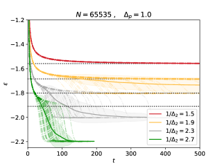
Refer to caption
Figure 10: Evolution of the loss in time from numerical simulations realised over 100 instances of disorder and noise, for the spiked matrix-tensor model with p=3𝑝3p=3. The simulations has been done with systems of size N=2161=65535𝑁superscript216165535N=2^{16}-1=65535 with parameters 1/Δ2{1.5,1.9,2.3,2.7}1subscriptΔ21.51.92.32.71/\Delta_{2}\in\{1.5,1.9,2.3,2.7\} and Δp=1.0subscriptΔ𝑝1.0\Delta_{p}=1.0.

In order to evaluate Gradient flow dynamics we discretized time and evaluated Eq. (4) numerically using effectively gradient descent

σit+1=μtσit(𝝈t|𝑻,𝒀)σit.superscriptsubscript𝜎𝑖𝑡1superscript𝜇𝑡superscriptsubscript𝜎𝑖𝑡conditionalsuperscript𝝈𝑡𝑻𝒀superscriptsubscript𝜎𝑖𝑡\sigma_{i}^{t+1}=-\mu^{t}\sigma_{i}^{t}-\frac{\partial\text{\large$\ell$}(\boldsymbol{\sigma}^{t}|\boldsymbol{T},\boldsymbol{Y})}{\partial\sigma_{i}^{t}}\,. (79)

In our experiments we run the dynamics on numerous realisations of the problem for different values of the parameters at p=3𝑝3p=3. Given a signal 𝝈𝕊N1superscript𝝈superscript𝕊𝑁1\boldsymbol{\sigma}^{*}\in\mathbb{S}^{N-1}, the number of computations per interaction scales as N3superscript𝑁3N^{3}, which makes the system hard to simulate for large N𝑁N. In order to increase the size of the system, we considered a diluted system, as proposed in [40], instead of the real system, such that the first and the second moment of the loss, in the leading order on N𝑁N. In the original system the (hyper)-graph of interaction is fully connected and counts N3/3!superscript𝑁33N^{3}/3! (hyper)-edges for the tensor and N2/2superscript𝑁22N^{2}/2 edges for the matrix. In the diluted systems we replace the (hyper)-graphs by graphs less connected in particular we take N2superscript𝑁2N^{2} (hyper)-edges for the tensor and NN𝑁𝑁N\sqrt{N} edges for the matrix. In systems with spherical variables there is a known problem [41] associated with reducing too much the number of interaction. In general given a tensor of order p𝑝p if the number of interaction becomes less then Np1superscript𝑁𝑝1N^{p-1} the system tends to favour a finite number of (hyper)-edges and aligns completely with them. The dynamics then converges to a final configuration where O(p)𝑂𝑝O(p) spins have value of order O(1)𝑂1O(1) and the rest is of order O(1/N)𝑂1𝑁O(1/\sqrt{N}). In order to have the same averages for the observables — such as overlap with the signal and loss — called #()#\#(\cdot) that counts the number of interactions, we multiplied the variances of the noise by N3/2/(3!#(𝑻))superscript𝑁323#𝑻N^{3/2}/(3!\#(\boldsymbol{T})) and N/(2#(𝒀))𝑁2#𝒀N/(2\#(\boldsymbol{Y})) respectively the tensor noise and the matrix noise.

Using this observation in the code we obtain a simple algorithm that given a dt𝑑𝑡dt approximate gradient flow by computing a gradient descent dynamics, with dt=1.0𝑑𝑡1.0dt=1.0 in the simulations. This value was chosen observing that in the runs the algorithm always descends in terms of loss and not appreciable difference appeared reducing it further. The code is made available and attached to this paper. Using this code we were able to simulate systems of the size N=2161=65535𝑁superscript216165535N=2^{16}-1=65535 and reduce finite size effects. Fig. 10 shows the average over different initialisation and realisation of the noise for the parameters presented in the paper Δp=1.0subscriptΔ𝑝1.0\Delta_{p}=1.0 and 1/Δ2{1.5,,1.9,,2.3,,2.7,}1/\Delta_{2}\in\{1.5,\,,1.9,\,,2.3,\,,2.7,\}. In the figure we use a continuous line surrounded by a shadow to represent mean and standard deviation under a Gaussian hypothesis, individual simulations are represented using dashed-dotted lines. For p=3𝑝3p=3 and Δp=1.0subscriptΔ𝑝1.0\Delta_{p}=1.0 the critical threshold for gradient flow occurs at 1/Δ2GF=2.01superscriptsubscriptΔ2GF2.01/\Delta_{2}^{\rm GF}=2.0 and in fact we observe that the green line (1/Δ2=1.91subscriptΔ21.91/\Delta_{2}=1.9) shows finite size effects and some simulations find good overlap with the ground truth. To conclude the figure shows a very good agreement with the averaged value evaluated using CHSCK equations, see Fig. 4-b. In particular is evident how all the dynamics tends to the threshold states, whose corresponding losses are drown with horizontal dotted lines, before eventually find the good direction and then the signal.