Improving Variational Quantum Optimization using CVaR

Abstract

Hybrid quantum/classical variational algorithms can be implemented on noisy intermediate-scale quantum computers and can be used to find solutions for combinatorial optimization problems. Approaches discussed in the literature minimize the expectation of the problem Hamiltonian for a parameterized trial quantum state. The expectation is estimated as the sample mean of a set of measurement outcomes, while the parameters of the trial state are optimized classically. This procedure is fully justified for quantum mechanical observables such as molecular energies. In the case of classical optimization problems, which yield diagonal Hamiltonians, we argue that aggregating the samples in a different way than the expected value is more natural. In this paper we propose the Conditional Value-at-Risk as an aggregation function. We empirically show – using classical simulation as well as quantum hardware – that this leads to faster convergence to better solutions for all combinatorial optimization problems tested in our study. We also provide analytical results to explain the observed difference in performance between different variational algorithms.

1 Introduction

Combinatorial optimization (CO) has been extensively studied, because it is applied in many areas of business and science, and it is a source of interesting mathematical problems [18]. Even if many CO problems are NP-hard, they are routinely solved (possibly not to provable optimality) in industrial applications. It is widely believed that quantum computers cannot solve such problems in polynomial time (i.e., NP $\not\subseteq$ BQP [5]), but there is significant effort toward designing quantum algorithms that could be practically useful by quickly finding near-optimal solutions to these hard problems. Among these algorithms, two candidates are more likely to be efficiently implementable on noisy quantum computers: the Variational Quantum Eigensolver (VQE) [16, 10], and the Quantum Approximate Optimization Algorithm (QAOA) [7, 9, 6]. Both VQE and QAOA use a parametrized quantum circuit $U(\theta)$ (also called variational form) to generate trial wave functions $\ket{\psi(\theta)}=U(\theta)\ket{0}$, guided by a classical optimization algorithm that aims to solve:

$$\min_{\theta}\bra{\psi(\theta)}H\ket{\psi(\theta)}.$$ (1)

This expression encodes the total energy of a system through its Hamiltonian $H$, and more specifically its expected value $\bra{\psi(\theta)}H\ket{\psi(\theta)}$. There is a well-known transformation to map CO problems into a Hamiltonian, see e.g., [15]; this will also be discussed subsequently in this paper. Empirical evaluations indicate that VQE’s performance suffers from some key weaknesses in the context of CO problems, and there is significant room for improvement [17]. At the same time, the literature on QAOA paints a mixed picture: while some work concludes that QAOA has promise [6, 19], other papers indicate that it may not perform better than classical algorithms [12].

In this paper, we propose a modification to the problem (1) that is given to the classical optimization algorithm: rather than minimizing the expected value $\bra{\psi(\theta)}H\ket{\psi(\theta)}$, we minimize its Conditional Value-at-Risk (CVaR) – a measure that takes into account only the tail of the probability distribution and is widely used in finance [3]. We argue that CVaR more closely matches the practical goal of heuristic solution methods for CO problems. We provide an analytical and numerical study, showing that the proposed methodology significantly improves performance and robustness of VQE and QAOA in the context of CO. As a byproduct of this analysis, we find that for small-depth circuits it is important to use variational forms with a sufficient number of parameters, e.g., at least linear in the number of qubits. QAOA for fixed (small) depth does not satisfy this requirement, and produces “flat” quantum states that yield low probability of sampling the optimal solution. Thus, not only does our paper introduce a simple way to improve the performance of the two most prominent candidates for CO on noisy quantum computers, but it also sheds some light on their behavior with small-depth circuits. While we do not claim that this brings their performance on par with state-of-the-art classical heuristics, our results indicate a marked improvement as compared to what is proposed in the literature. The numerical experiments discussed in this paper are implemented in the open-source library Qiskit [2], and executed on classical quantum simulators as well as IBM’s quantum hardware.

The rest of this paper is divided as follows. The next two sections set the context for this paper by giving an overview of key concepts from the literature: the mapping of CO problems as a Hamiltonian, VQE (Section 2), and QAOA (Section 3). Section 4 formally introduces our main contribution, CVaR optimization. An analysis of the method is given in Section 5. Section 6 provides an empirical evaluation of the proposed method on classically simulated quantum circuits, and using quantum hardware. Section 7 provides a formal analysis of certain aspects of QAOA to explain the experimentally observed behavior. Finally, Section 8 concludes the paper.

2 Variational Quantum Eigensolver

The Variational Quantum Eigensolver (VQE) is a hybrid quantum/classical algorithm originally proposed to approximate the ground state of a quantum chemical system, i.e., the state attaining the minimum energy [20]. This is achieved by solving a problem of the form (1), with $H$ encoding the total energy of the quantum chemical system. The same approach can be used to attempt to solve CO problems. Consider a quadratic unconstrained binary optimization (QUBO) problem on $n$ variables:

$$\min_{x\in\{0,1\}^{n}}b^{T}x+x^{T}Ax,$$ (2)

for given $b\in\mathbb{R}^{n}$ and $A\in\mathbb{R}^{n\times n}$. Using the variable transformation $x_{i}=(1-z_{i})/2$ for $z_{i}\in\{-1,+1\}$, problem (2) can be expressed as an Ising spin glass model:

$$\min_{z\in\{-1,+1\}^{n}}c^{T}z+z^{T}Qz,$$ (3)

where $c$ and $Q$ are easily computed from (2). These two equivalent problems encompass binary optimization problems, i.e., CO problems, and they are NP-hard [4].

Problem (3) can be translated into a Hamiltonian for an $n$-qubit system: we replace $z_{i}$ by the Pauli Z-matrix

$$\sigma_{Z}^{i} = \left(\begin{array}[]{cc}1&0\\ 0&-1\end{array}\right)$$ (6)

acting on the $i$-th qubit, and each term of the form $z_{i}z_{j}$ by $\sigma_{Z}^{i}\otimes\sigma_{Z}^{j}$. The summation of (tensor products of) Pauli terms obtained this way is the desired Hamiltonian. The eigenvalues $\pm 1$ of $\sigma_{Z}^{i}$ correspond to the positive and negative spin of (3). After constructing $H$, we can apply VQE to attempt to determine the ground state, from which an optimal solution to (3) can be sampled with probability 1.

The choice of the variational form $U(\theta)$ is important. In this paper we follow a standard approach, see e.g., [14, 17]. Assuming $n$ qubits, we start by applying single-qubit Y-rotations to every qubit, parametrized by an angle $\theta_{0,i}$ for qubit $i$. We then repeat the following $p$ times: we apply controlled Z-gates to all qubit pairs $(i,j)$ satisfying $i<j$, where $i$ denotes the control qubit and $j$ the target qubit; and we add another layer of single-qubit Y-rotations to every qubit, parametrized by $\theta_{k,i}$ for qubit $i$ and repetition $k\in\{1,\dots,p\}$. Fig. 1 illustrates such a variational form for $n=3$ and $p=2$. Notice that this variational form span all basis states. Overall, this leads to $n(1+p)$ parametrized Y-rotations, and $\frac{n(n-1)}{2}p$ controlled Z-gates. Since the controlled Z-gates commute with each other, the total circuit depth is $O(np)$, although the number of gates is quadratic in $n$. This variational form is used in our numerical simulations. When experimenting on quantum hardware we use nearest neighbor controlled Z-gates rather than all-to-all, i.e., we follow the connectivity provided by the hardware to reduce the number of two-qubit gates. We remark that these variational forms span any basis state (and thus the ground state of a diagonal Hamiltonian) already with the first layer of Y-rotations. The purpose of subsequent layers is to hopefully facilitate the task for the classical optimization algorithm used to choose the variational parameters. The above variational form with just one layer of Y-rotations can be efficiently simulated classically; for a discussion on the effect of entangling gates, we refer to [17].

Figure 1: VQE variational form for $n=3$ qubits and depth parameter $p=2$.

The classical optimization algorithm that attempts to solve (1) must be able to (at least) compute the objective function, i.e., the expected value in (1). This is difficult to compute directly, but it can be estimated as follows. First, we prepare the trial wavefunction $\ket{\psi(\theta)}$ on a quantum processor. Then, we measure the qubits, resulting in an $n$-bit string $x_{0}\dots x_{n-1}$. Each observed string easily translates into a sample from $\bra{\psi(\theta)}H\ket{\psi(\theta)}$, because $H$ is a weighted summation of tensor products of Pauli Z-matrices, and each such term can be computed with a simple parity check. We denote these samples by $H_{k}(\theta)$, $k=1,\dots,K$, where $K\in\mathbb{N}$ is the number of samples. The sample mean

$$\frac{1}{K}\sum_{k=1}^{K}H_{k}(\theta)$$ (7)

is an estimator for $\bra{\psi(\theta)}H\ket{\psi(\theta)}$, and is used as the objective function for the classical optimization algorithm. The solution returned by the algorithm is then given by the bitstring that leads to the smallest $H_{k}$ among all observed bitstrings and all $\theta$ that have been evaluated.

3 Quantum Approximate Optimization Algorithm

The Quantum Approximate Optimization Algorithm (QAOA) is a hybrid quantum/classical algorithm specifically developed for CO problems. In the context of this paper, QAOA can be seen as a form of VQE with a specific choice of the variational form that is derived from the problem Hamiltonian $H$ [7]. QAOA enjoys stronger convergence properties than VQE. For some problems, it can be shown that QAOA determines a quantum state with a guaranteed approximation ratio with respect to the ground state [7, 8]; furthermore, QAOA applies adiabatic evolution as the circuit depth goes to $\infty$, implying that it will determine the optimal solution of the CO problem if the depth of the variational form is large enough and we can find the optimal circuit parameters.

Given a problem Hamiltonian corresponding to a QUBO as defined in (3), the variational form of QAOA is constructed with a layer of Hadamard gates, followed by two alternating unitaries:

$$U_{C}(\gamma) = e^{-i\gamma\left(\sum_{i=1}^{n}c_{i}\sigma_{Z}^{i}+\sum_{i,j=1}^{n}Q_{ij}\sigma_{Z}^{i}\otimes\sigma_{Z}^{j}\right)},$$ (8)

$$U_{B}(\beta) = e^{-i\beta\sum_{i=1}^{n}\sigma_{X}^{i}},$$ (9)

where $\sigma_{X}^{i}$ denotes the Pauli X-matrix

$$\sigma_{X}^{i} = \left(\begin{array}[]{cc}0&1\\ 1&0\end{array}\right)$$ (12)

acting on the $i$-th qubit. For a given depth $p\in\mathbb{N}$, the variational form is thus defined as:

$$U(\beta,\gamma) = \left[\prod_{i=1}^{p}U_{B}(\beta_{i})U_{C}(\gamma_{i})\right]H^{\otimes n},$$ (13)

where $\beta,\gamma\in\mathbb{R}^{p}$ are vectors of variational parameters, and here, $H$ denotes a Hadamard gate. (The symbol $H$ is overloaded in the quantum computing literature; in this paper it generally denotes the Hamiltonian, and in the few occasions where it indicates a Hadamard gate, we note it explicitly.) This yields the trial wave function:

$$\ket{\psi(\beta,\gamma)} = U(\beta,\gamma)\ket{0},$$ (14)

which replaces $\ket{\psi(\theta)}$ in (1). As in VQE, the expected value is computed as the sample mean over multiple observations from the quantum state, and the algorithm returns the bitstring that leads to the smallest $H_{k}$ among all observed bitstrings and choices of $\beta,\gamma$.

The number of variational parameters for QAOA is thus $2p$, compared to $n(1+p)$ for VQE. The circuit depth of the QAOA variational form depends on $n$, $p$, and the number of clauses in the problem Hamiltonian, which is a difference with respect to VQE. Every $U_{B}$ requires $n$ single-qubit X-rotations. One way to construct $U_{C}$ requires a single-qubit Z-rotation for each $c_{i}\neq 0$, and a single-qubit Z-rotation plus two CNOT-gates for each $Q_{ij}\neq 0$, yielding the term $e^{-i\gamma\sigma_{Z}^{i}\otimes\sigma_{Z}^{j}}$ up to a global phase. The circuits used in our implementation are described in Appendix A. In total, this leads to $O(n^{2}p)$ single-qubit rotations and $O(n^{2}p)$ CNOT-gates, but the scaling may be better than the worst case if $Q$ is sparse (i.e., there are few two-qubit interactions).

4 CVaR Optimization

In quantum mechanics observables are defined as expected values $\bra{\psi}H\ket{\psi}$. This leads to the natural choice of the sample mean (7) as the objective function for the classical optimization problems embedded in VQE and QAOA. We argue that for problems with a diagonal Hamiltonian, such as CO problems, the sample mean may be a poor choice in practice. This is because when $H$ is diagonal, there exists a ground state which is a basis state. If determining the value $H_{j,j}$ of a basis state $\ket{j}$ is classically easy, the state with the minimum eigenvalue computed by an algorithm is simply the best measurement outcome among all measurements performed. It is therefore reasonable to focus on improving the properties of the best measurement outcome, rather than the average. We illustrate this intuition with a simple example. Consider two algorithms ${\cal A}_{1}$ and ${\cal A}_{2}$ applied to a problem with Hamiltonian $H$, minimum eigenvalue $\lambda_{\min}$ and ground state $\ket{j}$. Suppose ${\cal A}_{1}$ produces a state $\ket{\psi_{1}}$ and ${\cal A}_{2}$ produces a state $\ket{\psi_{2}}$, with the following properties: $\bra{\psi_{1}}H\ket{\psi_{1}}/\lambda_{\min}=1.1$ and $\braket{j}{\psi_{1}}=0$; $\bra{\psi_{2}}H\ket{\psi_{2}}/\lambda_{\min}=2.0$ and $\braket{j}{\psi_{2}}=0.1$. We argue that from a practical point of view, algorithm ${\cal A}_{2}$ is likely to be more useful than ${\cal A}_{1}$. This is because even if ${\cal A}_{1}$ leads to samples with a better objective function value on average, ${\cal A}_{1}$ will never yield the ground state $\ket{j}$; whereas ${\cal A}_{2}$, which is much worse on average, has a positive and sufficiently high probability of yielding the ground state, so that with enough repetitions we can be almost certain of determining $\ket{j}$.

In light of this discussion, one way to attain our goal would be to choose, as the objective function, the minimum observed outcome over a set of measurements: $\min\{H_{1},...,H_{K}\}$. However, for finite $K$ this typically leads to a non-smooth, ill-behaved objective function that is difficult to handle for classical optimization algorithms.

To help smooth the objective function, while still focusing on improving the best measured outcomes rather than the average, we propose the Conditional Value at Risk (CVaR, also called Expected Shortfall) as the objective function. Formally, the CVaR of a random variable $X$ for a confidence level $\alpha\in(0,1]$ is defined as

$$\text{CVaR}_{\alpha}(X) = \mathbb{E}[X|X\leq F_{X}^{-1}(\alpha)]$$ (15)

where $F_{X}$ denotes the cumulative density function of $X$. In other words, CVaR is the expected value of the lower $\alpha$-tail of the distribution of $X$. Without loss of generality, assume that the samples $H_{k}$ are sorted in nondecreasing order, i.e. $H_{k+1}\geq H_{k}$. Then, for a given set of samples $\{H_{k}\}_{k=1,\dots,K}$ and value of $\alpha$, the $\text{CVaR}_{\alpha}$ is defined as

$$\frac{1}{\lceil\alpha K\rceil}\sum_{k=0}^{\lceil\alpha K\rceil}H_{k}.$$ (16)

Note that the limit $\alpha\searrow 0$ corresponds to the minimum, and $\alpha=1$ corresponds to the expected value of $X$. In this sense, CVaR is a generalization of both the sample mean (7), and the best observed sample $\min\{H_{1},...,H_{K}\}$. For small, nonzero values of $\alpha$, CVaR still puts emphasis on the best observed samples, but it leads to a smoother and easier to handle objective function. It is clear that this can be applied to both VQE and QAOA, simply by replacing the sample mean (7) with $\text{CVaR}_{\alpha}$ in the classical optimization algorithm. We call the resulting algorithms CVaR-VQE and CVaR-QAOA, respectively.

5 Analysis of CVaR Optimization

The optimization of $\text{CVaR}_{\alpha}$ with $\alpha<1$ modifies the landscape of the objective function of VQE and QAOA as compared to the expected value, i.e., $\alpha=1$. This is formalized next.

We need to define a random variable that encodes the classical objective function value of a measurement outcome, i.e., the value of a binary string in the QUBO problem. Let $X(\theta)$ be the random variable with outcomes $H_{j,j}$ for $j\in\{0,1\}^{n}$, i.e., the diagonal elements of the Hamiltonian, and $\text{Prob}(X(\theta)=H_{j,j})=|\alpha_{j}(\theta)|^{2}$ where $\ket{\psi(\theta)}=\sum_{j}\alpha_{j}(\theta)\ket{j}$. In other words, $X(\theta)$ represents the QUBO objective function associated with a single measurement taken on the quantum state $\ket{\psi(\theta)}$. Then the CVaR-version of (1) can be written as:

$$\min_{\theta}\text{CVaR}_{\alpha}(X(\theta)).$$ (17)

As it turns out, there is no well-defined mapping between local minima of (1) and (17).

Proposition 5.1

A local minimum of (1) does not necessarily correspond to a local minimum of (17), and vice versa.

To show this, we first exhibit a local minimum of (1) that is not a local minimum of (17). Consider a two-qubit Hamiltonian $H=\text{diag}(0,1,1,2)$, and variational form depicted in Fig. 2.

@C=1em @R=.6em & H 1
R_Y(θ)

Figure 2: Variational form for the first part of Prop. 5.1. Here, $H$ indicates a Hadamard gate.

It is easy to verify that the quantum state constructed by this variational form is $\ket{\psi(\theta)}=\frac{1}{\sqrt{2}}(\cos\frac{\theta}{2},\sin\frac{\theta}{2},-\sin\frac{\theta}{2},\cos\frac{\theta}{2})$. Given the Hamiltonian, we have $\text{CVaR}_{1}(X(\theta))=\mathbb{E}[X(\theta)]=\cos^{2}\frac{\theta}{2}+\sin^{2}\frac{\theta}{2}=1$ independent of $\theta$, so every value of $\theta$ is a local (in fact, global) minimum. On the other hand, it is clear that for $\alpha<1$ there are values of $\theta$ that are not local minima: for example, with $\alpha=0.5$ doing the calculations shows that $\text{CVaR}_{0.5}(X(\theta))=\sin^{2}\frac{\theta}{2}$. Hence, the only local minima are at $\theta=2k\pi$ for $k$ integer.

The converse, i.e., a local minimum of (17) that is not a local minimum of (1), is trivial: for any problem (1) and parameters $\theta^{*}$ such that $\ket{\psi(\theta^{*})}$ has overlap $\rho>0$ with the ground state, $\theta^{*}$ is a global minimum of $\text{CVaR}_{\alpha}(X(\theta^{*}))$ for $\alpha\leq\rho$, even if $\theta^{*}$ is not a local minimum of (1).

It is easy to see from the above discussion on local minima that, in fact, we cannot even map global minima of problems (1) and (17) to each other. In fact, suppose a certain trial state $\ket{\psi(\theta)}$ has overlap $\rho$ with the ground state, then it is a global optimum of (17) for any $\alpha\leq\rho$. On the other hand, it is clear that it may not be a global optimum of (1), depending on the variational form chosen. However, a specific case of interest for this paper is that, in which the variational form is capable of reaching the ground state, and the Hamiltonian is diagonal; then the above discussion implies that a global optimum of Eq.(1) is also a global optimum of Eq.(17) for any $\alpha$.

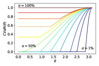
Even if Prop. 5.1 indicates that mapping properties of the optimization problems (1) and (17) is not trivial, the two-qubit example exhibiting a local minimum of (1) that is not a local minimum of (17) showcases a situation in which CVaR optimization is clearly preferrable. Indeed, using (1) yields a constant objective function on which no optimization can be performed. However, CVaR with $0<\alpha<1$ yields a smooth objective function that is optimized by decreasing $\theta$. This has a positive effect on the probability of sampling the ground state $\ket{00}$, which is maximized at $\theta=0$ in the interval $[0,\pi]$. The objective function (17) in this example for different values of $\alpha$ is illustrated in Fig. 3.

Figure 3: Objective function for different values of $\theta$ and $\alpha$: the top line corresponds to $\alpha=1$, the remaining lines show decreasing values of $\alpha$ down to $\alpha=0.01$ for the line in the bottom right.

It is important to remark that the natural empirical estimator of CVaR_α considers a subset of the measurements only. This raises the question of how to choose the number of samples for a particular value of $\alpha$ to achieve a certain accuracy. The variance of the empirical CVaR_α estimator using $K$ samples is $\mathcal{O}(1/(K\alpha^{2}))$ (see e.g., [13]), implying that the resulting standard error increases as $1/\alpha$. Thus, for a fixed number of samples $K$, to achieve the same accuracy as for the expected value we need to increase the number of samples to $K/\alpha$. (We remark that although [13] only shows this dependency for continuous distributions, we expect it to be a good approximation as the number of qubits increases.) As our numerical experiments show, $\alpha$ can be chosen as a constant, independent of the number of qubits, resulting in a constant increase of the number of samples for fixed accuracy. A discussion on the accuracy of the estimation from an empirical point of view is given in Sec. 6.

6 Computational experiments

The preceding analysis shows that CVaR optimization may improve certain properties of the classical optimization problem solved in VQE and QAOA. To verify if this is the case from an empirical point of view, we test the proposed on multiple random instances of six CO problems: maximum stable set, maximum 3-satisfiability, number partitioning, maximum cut, market split, and portfolio optimization. Below, we give a brief description of these problems. A more detailed discussion of the instance generation and the mapping to a Hamiltonian can be found in [17] for all problems except portfolio optimization, which is discussed in Appendix B.

Maximum stable set

Given an undirected graph $G=(V,E)$, a stable set (also called independent set) is a set of mutually nonadjacent vertices. The objective of the maximum stable set problem is to find a stable set of maximum cardinality.

Maximum 3-satisfiability

The objective of the maximum 3-satisfiability problem is to find an assignment of boolean variables that satisfies the largest number of clauses of a boolean formula in conjunctive normal form, where each clause has exactly three literals.

Number partitioning

Given a set of numbers $S=\{a_{1},...,a_{n}\}$, the problem of number partitioning asks to determine disjoint sets $P_{1},P_{2}\subset\{1,...,n\}$ with $P_{1}\cup P_{2}=\{1,...,n\}$, such that $\left|\sum_{i\in P_{1}}a_{i}-\sum_{j\in P_{2}}a_{j}\right|$ is minimized.

Maximum cut

Given a weighted undirected graph $G=(V,E)$ with edge weights $w_{ij}$, the maximum cut problem aims to determine a partition of $V$ into two disjoint sets $V_{1},V_{2}$ such that the sum of weights of edges that connect $V_{1}$ and $V_{2}$ is maximized.

Market split

The market split problem can be described as the problem of assigning $n$ customers of a firm that sells $m$ products to two subdivisions of the same firm, such that the two subdivisions retain roughly an equal share of the market.

Portfolio optimization

Given a set of $n$ assets $\{1,...,n\}$, corresponding expected returns $\mu_{i}$ and covariances $\sigma_{ij}$, a risk factor $q>0$ and a budget $B\in\{1,...,n\}$, the considered portfolio optimization problem tries to find a subset of assets $P\subset\{1,...,n\}$ with $|P|=B$ such that the resulting $q$-weighted mean-variance, i.e. $\sum_{i\in P}\mu_{i}-q\sum_{i,j\in P}\sigma_{ij}$, is maximized.

For each problem except Max3Sat, we generate ten random instances on $6,8,10,12,14$, and $16$ qubits. Our formulation of Max3Sat requires the number of qubits to be a multiple of three, thus we use $6,9,12$, and $15$ qubits. For every instance, we run CVaR-VQE and CVaR-QAOA for $\alpha\in\{1\%,5\%,10\%,25\%,50\%,75\%,100\%\}$ and $p=0,1,2$ for VQE and $p=1,2,3$ for QAOA. In total, this leads to 340 random problem instances and $14,280$ test cases. Following [17], we use the classical optimizer COBYLA to determine the parameters of the trial wave function.

In the first part of our experimental evaluation (Sec. 6.1), we analyze the performance of the different algorithms using the exact quantum state resulting from simulation. This allows us to precisely characterize the performance metrics that we use. In the second part (Sec. 6.2), we study the performance of the proposed approach using existing quantum hardware.

6.1 Results I: Simulation

We compare the different algorithms by plotting the resulting probability of sampling an optimal solution versus the number of iterations of the classical optimization algorithm. To make the number of iterations comparable for problems of different sizes, we normalize it dividing by the number of qubits. We choose the probability of sampling an optimal solution, rather than some aggregate measure of the objective function value, because all our algorithms use different metrics in this respect: comparing algorithms with respect to the average objective function value (or CVaR with a different $\alpha$) would not be informative. The probability of sampling an optimal solution (i.e., the overlap with ground state) is a reasonable metric that provides valuable information across different values of $\alpha$.

Fig. 4 shows the fraction of instances that achieve at least a certain probability of sampling an optimal state ($\geq 1\%$ and $\geq 10\%$) with respect to the number of normalized iterations for CVaR-VQE / CVaR-QAOA (using all-to-all entanglement). This fraction is shown for each considered variational form depth, $p$, and value of $\alpha$. The plots show that increasing $p$ and decreasing $\alpha$ has a positive impact on the performance.

For CVaR-VQE, using $p=2$ and $\alpha=1\%$, within 50 normalized iterations we achieve at least $1\%$ probability of sampling an optimal state for almost all instances. In contrast, with $\alpha=100\%$ (i.e., the expected value), we reach the same probability of sampling an optimum only for $60\%$ of the test problems. Notice that the value of $\alpha$ introduces a soft cap on the maximum probability of sampling a ground state: for example, for $\alpha=10\%$ we reach $10\%$ probability to sample an optimal solution for most of the test problems in less than 50 normalized iterations, but with $\alpha=1\%$ we reach $10\%$ probability only in a small fraction of problems. This is expected, because the CVaR objective function with $\alpha=1\%$ does not reward increasing the overlap with the ground state beyond 1% probability.

Figure 4: Summary of the results with VQE (left) / QAOA (right) using quantum states resulting from classical simulation. On the $x$-axis we plot the normalized number of iterations, on the $y$-axis the fraction of the instances that attain a certain probability of sampling an optimal basis state. Each plot contains results for different levels of $\alpha$ (reported as $aX\%$ in the legend), and the depth increases from top to bottom.

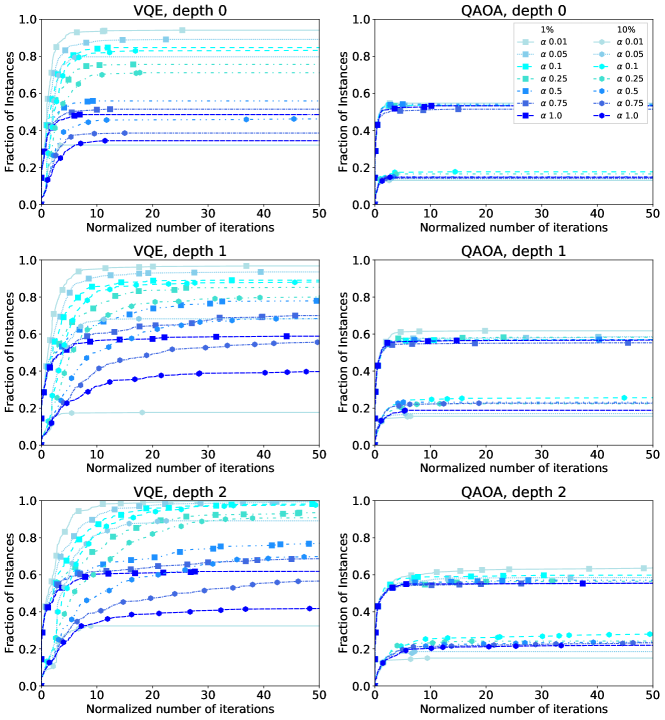
For CVaR-QAOA, we observe improved performance as $p$ increases and $\alpha$ decreases (up to a certain level). Comparing VQE and QAOA, we observe that QAOA’s performance appears significantly worse than that of VQE for equivalent depth (where we compare depth $p$ for VQE to depth $p+1$ for QAOA). We conjecture that this is due to the limited number of variational parameters in QAOA: only $2p$, compared to $n(1+p)$ for VQE. An intuitive explanation is that the state vector obtained with QAOA is thus relatively “flat”, and never reaches a large overlap with the ground state. This intuitive explanation is formalized in Sec. 7. In the context of this paper, one of QAOA’s characteristics, i.e., the concentration around the mean [7], may become a weakness in the practical context of sampling the optimum (or a near-optimal solution) with sufficiently large probability. To improve QAOA’s performance we would have to increase the depth. Since the current generation of quantum hardware is affected by non-negligible gate errors and decoherence, successfully implementing circuits with large depth may be out of reach for the moment.

Figure 5: Summary of the results with VQE (left) / QAOA (right) using quantum states resulting from classical simulation, after 50 normalized iterations of the classical optimization algorithm. On the vertical $z$-axis we plot the fraction of instances that attain $10\%$ probability of sampling the optimal solution, on the $xy$-plane we indicate the number of qubits and the value of $\alpha$.

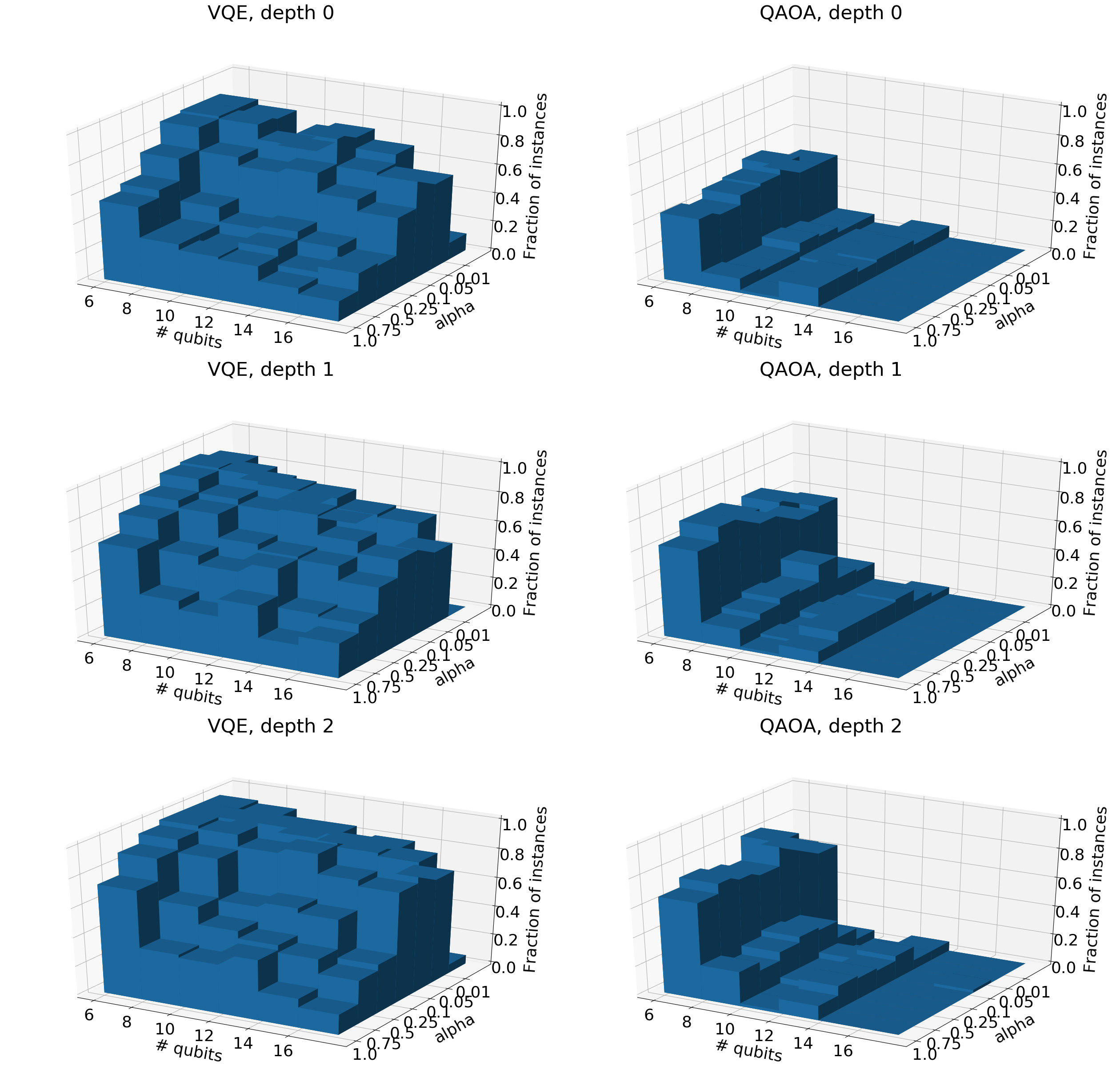
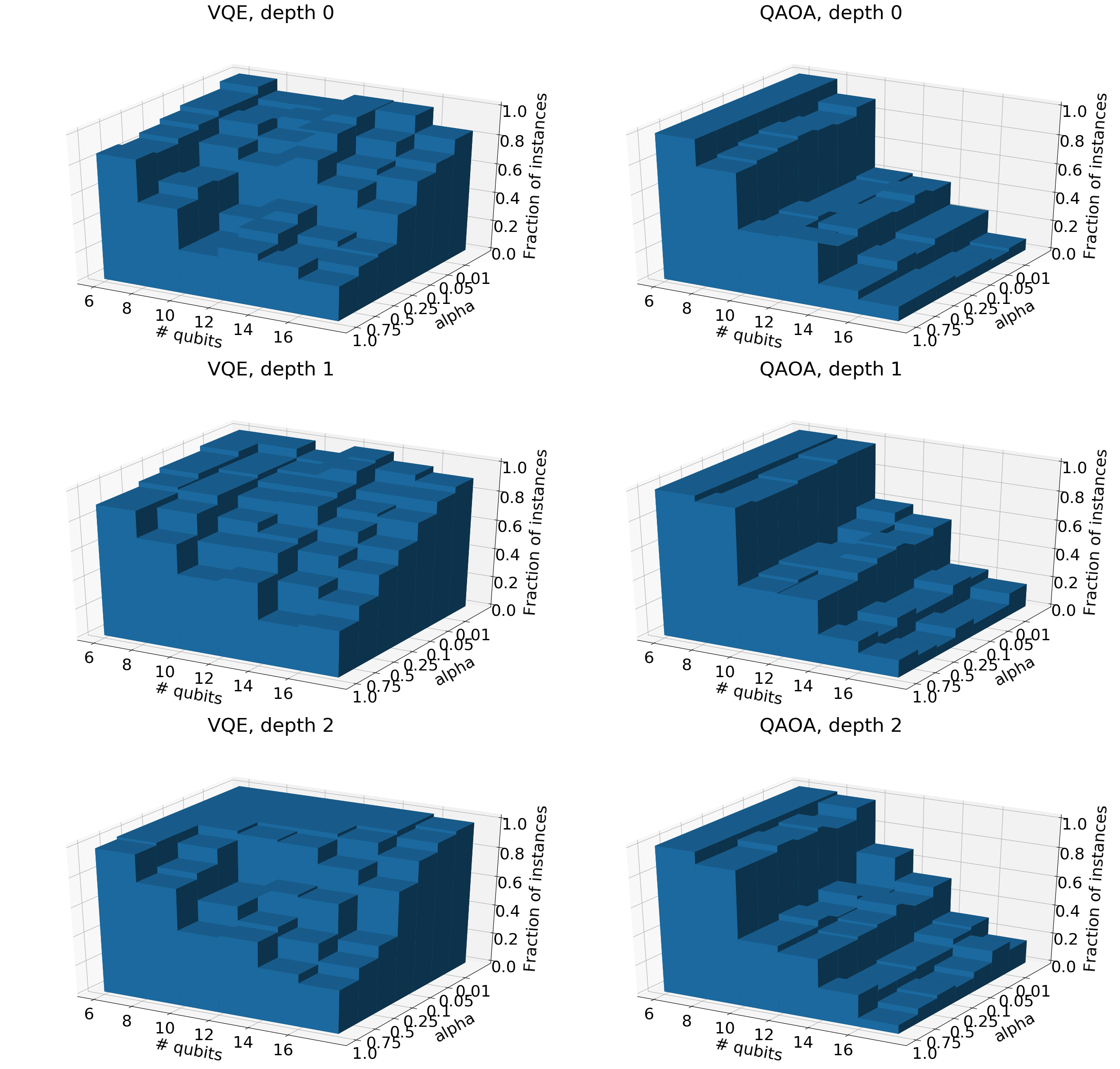
To ensure that the positive effect of CVaR optimization is not lost when the problem size increases, we look at the results across different number of qubits and values of $\alpha$. The corresponding plots are given in Fig. 5 for a probability of sampling the optimum of 10%; a similar figure for 1% probability is available in Appendix C. Fig. 5 shows that for a small number of qubits there is a ceiling effect, i.e., all methods perform similarly because the problem is easy for all methods, but as soon as problem size increases, the benefits of CVaR optimization (with $\alpha\in[0.01,0.25]$) are obvious in the plots.

6.2 Results II: Quantum Device

To test CVaR optimization on quantum hardware, we consider an instance of the portfolio optimization problem with 6 assets mapped to 6 qubits, see Appendix B. We choose portfolio optimization because the problems of this class are some of the most difficult of our testbed.

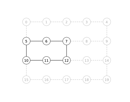
We test CVaR-VQE on the IBM Q Poughkeepsie 20-qubit quantum computer, with COBYLA as the classical optimizer. In this section we apply nearest neighbor entanglement instead of all-to-all entanglement. We choose 6 qubits on the device that are connected in a ring (qubits 5, 6, 7, 10, 11, and 12), thus achieving a cyclic entanglement without additional swap operations; see Appendix B for more detail. We use CVaR-VQE rather than CVaR-QAOA because for the same circuit depth it leads to better solutions, as discussed in Sec. 6.1.

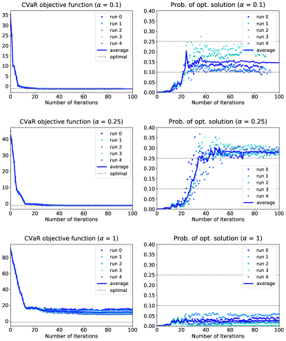
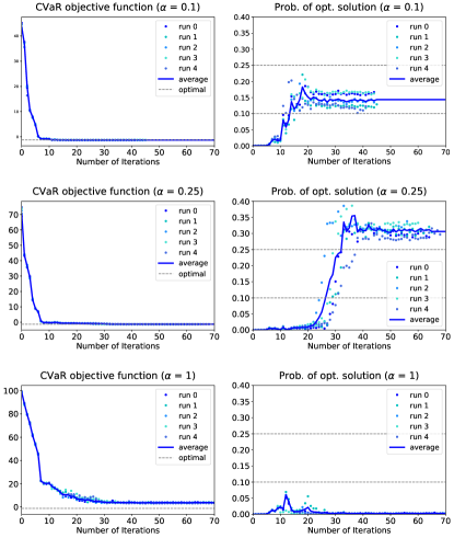
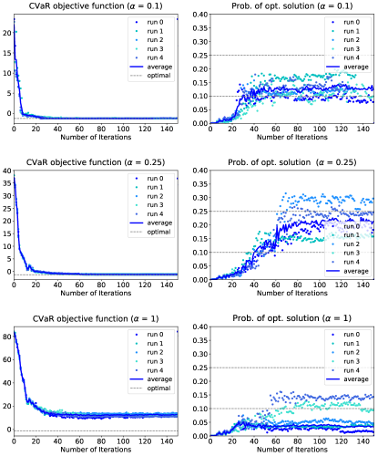
We run CVaR-VQE with depth $p=1$ and $\alpha=10\%,25\%,100\%$, repeating each experiment five times. We gather 8,192 samples from each trial wavefunction, studying the probability of measuring a ground state with respect to the number of iterations of the classical optimization algorithm. To illustrate the convergence of the algorithm, we also plot the progress in the objective function value. Note that the reported objective function values for different values of $\alpha$ are incomparable. To reduce variance in the experiments, we fix the initial variational parameters to $\theta=0$. Results are reported in Fig. 6. Similar plots for depth $p=0$ and $p=2$ are given in Appendix B.

We see that the smaller the $\alpha$, the earlier the probability of sampling an optimal solution increases. For $\alpha=100\%$, the probability stays almost flat and makes little progress. The plots of the objective function also show that $\alpha<100\%$ speeds up the convergence of the objective function values to a (local) optimum. For $\alpha=10\%,25\%$ the probability of finding the optimal solution attains the corresponding $\alpha$-level in all 5 experiments, whereas for $\alpha=100\%$ the probability remains very small. Recall that the CVaR objective function does not provide any incentive to increase the overlap with the optimal solution beyond $\alpha$.

Figure 6: Quantum hardware results for portfolio optimization problem with six assets/qubits. CVaR-VQE results are shown for depth $p=1$ and $\alpha=10\%,25\%,100\%$ (from top to bottom) and five runs with 8,192 samples for each $\alpha$. Plots on the left: resulting objective values per iteration; plots on the right: resulting probability of sampling an optimal solution. Since COBYLA converges after a different number of iterations in each run, we assume that the contribution of each run to the average value after termination of that run is its last reported value. The $\alpha$-levels $10\%$ and $25\%$ are indicated by the gray dashed lines in all probability plots.

In addition to the improved convergence behavior already demonstrated in Sec. 6.1 using classical simulation, the CVaR objective function also seems to be able to cope with the noise and errors introduced by the quantum hardware. Indeed, on quantum hardware we observe the same beneficial effect on the speed of convergence that was observed in the noiseless simulation results. A possible explanation is that the CVaR objective function allows us to ignore some of the low-quality samples from the quantum state. In other words, even if we do not reach the ground state (which may be difficult to detect in the presence of noise), CVaR focuses on ensuring that at least some of the samples have a low objective function value, which may be a more attainable goal and seems to drive the classical optimization algorithm in the right direction. This effect makes the CVaR objective particularly well-suited for experiments on noisy quantum computers.

We end this section with a discussion on the impact of $\alpha$ on the number of samples. As discussed in Sec. 5, to obtain the same accuracy as the expected value we would need to increase the number of samples by a factor $\frac{1}{\alpha}$. Results in this paper suggest choosing $\alpha\in[0.1,0.25]$ as a good empirical choice, implying that the number of samples should be increased by a factor $[4,10]$ to attain the same accuracy. However, our empirical evaluation uses the same, fixed number of samples across all $\alpha$, and still shows significant benefits of CVaR optimization. A possible explanation is that as long as the number of samples allows a reasonable estimation of the CVaR objective function, the loss in estimation accuracy (as compared to the expected value) is counterbalanced by the fact that the CVaR objective is more effective at guiding the classical optimization algorithm toward a quantum state that overlaps with the optimal solution. Thus, in our empirical evaluation even a noisy CVaR estimate yields better results than a more accurate expected value estimate.

7 On the performance of QAOA

In this section we formalize our intuition that, due to the small number of variational parameters, QAOA may produce relatively “flat” state vectors, i.e., with amplitudes of similar magnitude. We initially observed this behavior empirically, and it can be made precise under some additional conditions.

Proposition 7.1

Assume that we apply QAOA to a problem on $n$ qubits with objective function encoded in a diagonal Hamiltonian $H$ with diagonal elements $H_{j,j},j=1,\dots,2^{n}$. Let $\delta:=\max_{\ell}|\{j\in\{0,1\}^{n}:H_{j,j}=\ell\}|/2^{n}$, i.e., the maximum fraction of basis states having the same eigenvalue. Let $\ket{\psi_{p}}=\sum_{z}\alpha_{p,z}\ket{z}$ be the quantum state produced by QAOA with depth $p$. Let $\Delta_{p}$ be a lower bound on the maximum fraction of amplitudes that are equal after iteration $p$ of QAOA, i.e., $\Delta_{p}:=\min_{t\leq p}\max_{u\in\mathbb{C}}|\{j\in\{0,1\}^{n}:\alpha_{t,j}=u\}|/2^{n}$. Then $|\alpha_{p,z}|\leq(2^{n+1}(2-\Delta_{p-1}-\delta)+1)^{p}\frac{1}{\sqrt{2^{n}}}$ for all $z\in\{0,1\}^{n}$. Furthermore, $\Delta_{0}=1$, but the value of $\Delta_{p}$ may decrease exponentially fast in $p$.

The proof of the above proposition is given in Appendix D. While the statement is technical, we discuss some special cases that provide an intuition. When $p=1$ and most of the diagonal values of the Hamiltonian are equal, say, $\delta\geq 1-2^{-n(\frac{1}{2}+\epsilon)}$, $\epsilon>0$, then the resulting state vector is necessarily flat: all the amplitudes are exponentially small $O(\frac{1}{2^{\epsilon n}})$. This situation is easy to envision: when the Hamiltonian does not provide enough information on the distribution of objective function values, QAOA with small depth cannot transfer enough probability mass to any basis state. This is the case, for instance, in the Grover “needle in a haystack” problem [11] where a unique $z^{*}$ has objective function value $H_{z^{*},z^{*}}=1$ and $H_{z,z}=0$ for all other $z\in\{0,1\}^{n}$. Another example is given by the feasibility version of the market split problems, see the analysis on the number of solutions in [1]. The Hamiltonians that necessarily lead to flat state vectors are those with $\delta,\Delta_{p}\geq 1-2^{-n(\frac{1}{2}+\epsilon)}$; notice that intuitively, $\delta\approx 1$ is more likely to lead to $\Delta_{p}\approx 1$, although our proof in Appendix D shows a very loose lower bound on $\Delta_{p}$ that is exponentially decreasing in $p$. Another way to interpret Prop. 7.1 is that QAOA requires the diagonal elements of the Hamiltonian (i.e., objective function values) to be well-distributed to effectively “mix” and increase the amplitudes. This can also be achieved increasing $p$, say, linearly in $n$, but for fixed $p$ there is the risk that the amplitudes remain flat. While this may still lead to a good average objective function value, it may not put enough emphasis on the tail of the distribution of objective function values to sample an optimal or a near-optimal solution. Notice that examples of this are also discussed in the seminal paper [7]: the paper shows that for MaxCut on 2-regular graphs, QAOA produces a state with approximation ratio $3/4$ but exponentially small overlap with the optimal solution.

8 Conclusions

We introduce improved versions of the hybrid quantum/classical algorithms VQE and QAOA for CO, based on the CVaR aggregation function for the samples obtained from trial wavefunctions. We provide theoretical and empirical results, showing an increase in performance compared to approaches in the literature. This includes a demonstration on IBM’s quantum hardware, where the algorithm that we propose shows the ability to reach an optimal solution much faster.

Code Availability

A notebook providing the code to run CVaR-VQE is available open source at https://github.com/stefan-woerner/cvar_quantum_optimization/

Appendix A Implementation of QAOA

As discussed in the main text, implementing the blocks $U_{B}$ and $U_{C}$ of QAOA requires both single-qubit rotations and CNOT-gates. The implementation of $U_{B}$ is trivial in Qiskit, as X-rotations $R_{X}$ are natively supported, we can apply $R_{X}(-2\beta)$ to each qubit to implement $U_{B}$. For $U_{C}$, a possible implementation for $e^{-i\gamma\sigma_{Z}^{i}\otimes\sigma_{Z}^{j}}$ up to a global phase is depicted in Fig. 7 using two CNOT-gates and one single-qubit Z-rotation $R_{Z}$ (both also natively supported in Qiskit).

@C=1em @R=.6em & 1 1
R_Z(-2γ)

Figure 7: Implementation of $e^{-i\gamma\sigma_{Z}^{i}\otimes\sigma_{Z}^{j}}$ up to a global phase.

Appendix B Portfolio Optimization on Quantum Device

The portfolio optimization problem considered in Sec. 6.2 is given by

$$\max_{x\in\{0,1\}^{n}}\sum_{i=1}^{n}\mu_{i}x_{i}-q\sum_{i,j=1}^{n}\sigma_{ij}x_{i}x_{j}-\lambda\left(B-\sum_{i=1}^{n}x_{i}\right)^{2},$$

where we subtract a penalty term weighted by $\lambda$ to enforce the budget constraint $\sum_{i=1}^{n}x_{i}=B$. We choose $n=6$, $q=0.5$, $B=3$, and $\lambda=12$. The used return vector $\mu$ and positive semidefinite covariance matrix $\sigma$ were generated randomly and are given by:

$$\tiny\mu\tiny=\left(\begin{array}[]{cccccc}0.7313&0.9893&0.2725&0.8750&0.7667&0.3622\end{array}\right)$$

$$\tiny\sigma\tiny=$$

$$\tiny\left(\begin{array}[]{rrrrrr}0.7312&-0.6233&0.4689&-0.5452&-0.0082&-0.3809\\ -0.6233&2.4732&-0.7538&2.4659&-0.0733&0.8945\\ 0.4689&-0.7538&1.1543&-1.4095&0.0007&-0.4301\\ -0.5452&2.4659&-1.4095&3.5067&0.2012&1.0922\\ -0.0082&-0.0733&0.0007&0.2012&0.6231&0.1509\\ -0.3809&0.8945&-0.4301&1.0922&0.1509&0.8992\end{array}\right)$$

The corresponding Hamiltonian can be constructed as described e.g. in Sec. 2 and the references mentioned therein.

The variational form is constructed as described in Sec. 2 with nearest neighbor entanglement. The topology of IBM Q Poughkeepsie, the selected qubits and the entanglement are illustrated in Fig. 8.

Figure 8: Connectivity of IBM Q Poughkeepsie. We use qubits 5, 6, 7, 10, 11, and 12, and entangle nearest neighbors, i.e., we achieve a cyclic entanglement for every layer in the considered variational form.

In the remainder of this section, we report results for depth $p=0$ and $p=2$; for the overall setup, as well as results for $p=1$, see Section 6.2.

For $p=0$, Fig. 9 shows that results for $\alpha=10\%$ and $\alpha=25\%$ are similar to those for $p=1$. However, for $\alpha=100\%$ the probability of sampling a ground state first increases to $5\%$ on average, then it drops close to zero, even though the objective function improves. This is an example where improving the objective value does not necessarily imply getting a better overall solution (i.e., binary string), and highlights our motivation of using CVaR as the objective in contrast to the expected value.

Figure 9: Quantum hardware results for portfolio optimization problem with six assets/qubits. CVaR-VQE results are shown for depth $p=0$ and $\alpha=10\%,25\%,100\%$ (from top to bottom) and five runs with 8,192 samples for each $\alpha$. Plots on the left: resulting objective values per iteration; plots on the right: resulting probability of sampling an optimal solution. Since COBYLA converges after a different number of iterations in each run, we assume that the contribution of each run to the average value after termination of that run is its last reported value. The $\alpha$-levels $10\%$ and $25\%$ are indicated by the gray dashed lines in all probability plots.

For $p=2$, Fig. 10 again shows that results for $\alpha=10\%$ are similar to those for $p=0,1$. Although the probability of sampling a ground state is not always exceeding $\alpha$ as before, it reaches that level on average. However, for $\alpha=25\%$ the probability of sampling a ground state does not reach $\alpha$ anymore, but plateaus slightly below. For the expected value, i.e., $\alpha=100\%$, we again see a probability of the ground state which is close to zero and that decreases after an initial small increase.

Figure 10: Quantum hardware results for portfolio optimization problem with six assets/qubits. CVaR-VQE results are shown for depth $p=2$ and $\alpha=10\%,25\%,100\%$ (from top to bottom) and five runs with 8,192 samples for each $\alpha$. Plots on the left: resulting objective values per iteration; plots on the right: resulting probability of sampling an optimal solution. Since COBYLA converges after a different number of iterations in each run, we assume that the contribution of each run to the average value after termination of that run is its last reported value. The $\alpha$-levels $10\%$ and $25\%$ are indicated by the gray dashed lines in all probability plots.

Appendix C Additional plots

Fig. 11 shows additional results for VQE and QAOA for different values of $\alpha$, different numbers of qubits, and an overlap with the optimal solution of $1\%$.

Figure 11: Summary of the results with VQE (left) / QAOA (right) using quantum states resulting from classical simulation, after 50 normalized iterations of the classical optimization algorithm. On the vertical $z$-axis we plot the fraction of instances that attain $1\%$ probability of sampling the optimal solution, on the $xy$-plane we indicate the number of qubits and the value of $\alpha$.

Appendix D Proof of Proposition 7.1

We show this by induction on $p$. Let $u_{p}$ be the $\arg\max$ in the definition of $\Delta_{p}$ for $t=p$. With $p=0$, QAOA only applies a layer of Hadamard gates, therefore it is obvious that $|\alpha_{0,z}|=\frac{1}{\sqrt{2^{n}}}$. We now show the induction step. Recall that the $p+1$-th layer of QAOA applies two unitaries $U_{C}(\gamma),U_{B}(\beta)$ to the state $\ket{\psi_{p}}$, in the given order. Here, the objective function value of a basis state $\ket{z}$ is denoted $H_{z,z}$ for consistency with the rest of the paper. In classical QAOA notation, it is typically denoted $C(z):=\sum_{k=1}^{m}C_{k}(z)$, with $C_{k}(z)=0$ if string $z$ does not satisfy the $k$-th clause, $C_{k}(z)=1$ otherwise, and the goal is to maximize $C(z)$. We can simply think of $H$ as encoding $C$, i.e., $H_{z,z}=C(z)$. Let $\ket{\phi}$ be the state obtained after applying $U_{C}(\gamma)$. We have:

$$\ket{\phi} =U_{C}(\gamma)\ket{\phi_{p}}=\sum_{z}\alpha_{p,z}e^{-i\gamma H_{z,z}}\ket{z}.$$

Finally we apply $U_{B}(\beta)=(e^{-i\beta X})^{\otimes n}$ to obtain the state $\ket{\psi}=\sum_{z}\alpha_{p+1,z}\ket{z}$. Let $e^{-i\beta X}=\begin{pmatrix}a_{00}&a_{01}\\ a_{10}&a_{11}\end{pmatrix}$. By definition, for every basis state $\ket{j}$, we have:

$$\alpha_{p+1,j}= \sum_{z}\prod_{h=1}^{n}a_{j_{h}z_{h}}\alpha_{p,z}e^{-i\gamma H_{z,z}}$$ (20)

$$= \sum_{z}\prod_{h=1}^{n}a_{j_{h}z_{h}}\alpha_{p,z}e^{-i\gamma\ell}+$$

$$\sum_{z}\prod_{h=1}^{n}a_{j_{h}z_{h}}\alpha_{p,z}e^{-i\gamma\ell}\Big{(}e^{-i\gamma(H_{z,z}-\ell)}-1\Big{)}$$

$$= \sum_{z}\prod_{h=1}^{n}a_{j_{h}z_{h}}u_{p}e^{-i\gamma\ell}+$$

$$\sum_{z}\prod_{h=1}^{n}a_{j_{h}z_{h}}(\alpha_{p,z}-u_{p})e^{-i\gamma\ell}+$$

$$\sum_{z}\prod_{h=1}^{n}a_{j_{h}z_{h}}\alpha_{p,z}e^{-i\gamma\ell}\Big{(}e^{-i\gamma(H_{z,z}-\ell)}-1\Big{)}$$

$$= \big{(}(a_{00}+a_{01})^{\sum_{h}j_{h}}(a_{10}+a_{11})^{n-\sum_{h}j_{h}}$$

$$u_{p}e^{-i\gamma\ell}\big{)}+$$

$$\sum_{z}\prod_{h=1}^{n}a_{j_{h}z_{h}}(\alpha_{p,z}-u_{p})e^{-i\gamma\ell}+$$

$$\sum_{z}\prod_{h=1}^{n}a_{j_{h}z_{h}}\alpha_{p,z}e^{-i\gamma\ell}\Big{(}e^{-i\gamma(H_{z,z}-\ell)}-1\Big{)}.$$

So

$$|\alpha_{p+1,j}|\leq$$

$$\left|(a_{00}+a_{01})^{\sum_{h}j_{h}}(a_{10}+a_{11})^{n-\sum_{h}j_{h}}u_{p}e^{-i\gamma\ell}\right|+$$

$$\left|\sum_{z}\prod_{h=1}^{n}a_{j_{h}z_{h}}(\alpha_{p,z}-u_{p})e^{-i\gamma\ell}\right|+$$

$$\left|\sum_{z}\prod_{h=1}^{n}a_{j_{h}z_{h}}\alpha_{p,z}e^{-i\gamma\ell}\Big{(}e^{-i\gamma(H_{z,z}-\ell)}-1\Big{)}\right|.$$

Recalling that $a_{00}=a_{11}=\cos\beta,a_{01}=a_{10}=-i\sin\beta$, and $|u_{p}|\leq\max|\alpha_{p,z}|$, it follows that

$$\left|(a_{00}+a_{01})^{\sum_{h}j_{h}}(a_{10}+a_{11})^{n-\sum_{h}j_{h}}u_{p}e^{-i\gamma\ell}\right|\leq$$

$$\max_{z}|\alpha_{p,z}|.$$

We also have:

$$\left|\sum_{z}\prod_{h=1}^{n}a_{j_{h}z_{h}}(\alpha_{p,z}-u_{p})e^{-i\gamma\ell}\right|=$$

$$\left|\sum_{z:\alpha_{p,z}\neq u_{p}}\prod_{h=1}^{n}a_{j_{h}z_{h}}(\alpha_{p,z}-u_{p})e^{-i\gamma\ell}\right|\leq$$

$$2^{n}(1-\Delta_{p})\left|\prod_{h=1}^{n}a_{j_{h}z_{h}}\right|\left|(\alpha_{p,z}-u_{p})\right|\left|e^{-i\gamma\ell}\right|\leq$$

$$2^{n}(1-\Delta_{p})(\left|\alpha_{p,z}\right|+\left|u_{p}\right|)\leq$$

$$2^{n}(1-\Delta_{p})(2\max_{z}|\alpha_{p,z}|).$$

We now need to find an upper bound to the term $\left|\sum_{z}\prod_{h=1}^{n}a_{j_{h}z_{h}}\alpha_{p,z}e^{-i\gamma\ell}(e^{-i\gamma(H_{z,z}-\ell)}-1)\right|$. We obtain:

$$\left|\sum_{z}\prod_{h=1}^{n}a_{j_{h}z_{h}}\alpha_{p,z}e^{-i\gamma\ell}(e^{-i\gamma(H_{z,z}-\ell)}-1)\right|\leq$$

$$\sum_{z}\prod_{h=1}^{n}\left|a_{j_{h}z_{h}}\alpha_{p,z}e^{-i\gamma\ell}\right|\left|(e^{-i\gamma(H_{z,z}-\ell)}-1)\right|\leq$$

$$\sum_{z}|\alpha_{p,z}|\left|(e^{-i\gamma(H_{z,z}-\ell)}-1)\right|\leq$$

$$\max_{z}|\alpha_{p,z}|\sum_{z:H_{z,z}=\ell}\left|(e^{-i\gamma(\ell-\ell)}-1)\right|+$$

$$\max_{z}|\alpha_{p,z}|\sum_{z:H_{z,z}\neq\ell}\left|e^{-i\gamma(H_{z,z}-\ell)}-1\right|\leq$$

$$2\max_{z}|\alpha_{p,z}|2^{n}(1-\delta)$$

Thus, we have

$$|\alpha_{p+1,j}| \leq(2^{n+1}(2-\Delta_{p}-\delta)+1)\max_{z}|\alpha_{p,z}|$$

$$\leq(2^{n+1}(2-\Delta_{p}-\delta)+1)^{p+1}\frac{1}{\sqrt{2^{n}}},$$

where we used the fact that $\Delta_{p}$ is decreasing in $p$ by definition. It is also useful to determine a lower bound on $\Delta_{p}$. It is clear that $\Delta_{0}=1$ because for $p=0$ all amplitudes are equal. To find a lower bound on $\Delta_{p+1}$ based on $\Delta_{p}$, we look at the last line of (20), which decomposes $\alpha_{p+1,j}$ into three summations. The first summation has $n$ possible different values. The second summation has at most $\frac{n^{2}}{4}$ possible coefficient values for each $z$: this is because $\prod_{h=1}^{n}a_{j_{h}z_{h}}$ can be computed by looking at which $z_{h}$ are 1 and counting how many corresponding $j_{h}$ are 1, then doing the same for zeros. The largest number of combinations is obtained when $z$ has $n/2$ bits equal to 1, yielding $(n/2)^{2}$ combinations. Since there are $(1-\Delta_{p})2^{n}$ nonzero terms in the summation, in total we obtain at most $(n^{2}/4)^{(1-\Delta_{p})2^{n}}$ different values. The third summation is similar: $\frac{n^{2}}{4}$ possible coefficient values for each $z$, and $(1-\delta)2^{n}$ nonzero terms, for a total of at most $(n^{2}/4)^{(1-\delta)2^{n}}$ different values. In total, there are at most $n(n^{2}/4)^{(2-\delta-\Delta_{p})2^{n}}$ different values of $\alpha_{j}$. Hence, $\Delta_{p+1}\geq 1/(n(n^{2}/4)^{(2-\delta-\Delta_{p})2^{n}})$. With algebraic manipulations, we obtain a (possibly very loose) bound $\Delta_{p}\geq(\frac{1}{n^{3}})^{2^{n}(1-\delta+\frac{p-1}{p})}$ whenever $p\geq 1$.

References

- Aardal et al. [2000] Karen Aardal, Robert E Bixby, Cor AJ Hurkens, Arjen K Lenstra, and Job W Smeltink. Market split and basis reduction: Towards a solution of the cornuéjols-dawande instances. INFORMS Journal on Computing, 12(3):192–202, 2000. ISSN 1091-9856. doi: 10.1287/ijoc.12.3.192.12635.
- Abraham et al. [2019] Héctor Abraham, Ismail Yunus Akhalwaya, Gadi Aleksandrowicz, Thomas Alexander, Gadi Alexandrowics, Eli Arbel, Abraham Asfaw, Carlos Azaustre, AzizNgoueya, Panagiotis Barkoutsos, George Barron, Luciano Bello, Yael Ben-Haim, Daniel Bevenius, Lev S. Bishop, Sorin Bolos, Samuel Bosch, Sergey Bravyi, David Bucher, Fran Cabrera, Padraic Calpin, Lauren Capelluto, Jorge Carballo, Ginés Carrascal, Adrian Chen, Chun-Fu Chen, Richard Chen, Jerry M. Chow, Christian Claus, Christian Clauss, Abigail J. Cross, Andrew W. Cross, Simon Cross, Juan Cruz-Benito, Chris Culver, Antonio D. Córcoles-Gonzales, Sean Dague, Tareq El Dandachi, Matthieu Dartiailh, DavideFrr, Abdón Rodríguez Davila, Delton Ding, Jun Doi, Eric Drechsler, Drew, Eugene Dumitrescu, Karel Dumon, Ivan Duran, Kareem EL-Safty, Eric Eastman, Pieter Eendebak, Daniel Egger, Mark Everitt, Paco Martín Fernández, Axel Hernández Ferrera, Albert Frisch, Andreas Fuhrer, MELVIN GEORGE, Julien Gacon, Gadi, Borja Godoy Gago, Jay M. Gambetta, Adhisha Gammanpila, Luis Garcia, Shelly Garion, Juan Gomez-Mosquera, Salvador de la Puente González, Jesse Gorzinski, Ian Gould, Donny Greenberg, Dmitry Grinko, Wen Guan, John A. Gunnels, Mikael Haglund, Isabel Haide, Ikko Hamamura, Vojtech Havlicek, Joe Hellmers, Łukasz Herok, Stefan Hillmich, Hiroshi Horii, Connor Howington, Shaohan Hu, Wei Hu, Haruki Imai, Takashi Imamichi, Kazuaki Ishizaki, Raban Iten, Toshinari Itoko, Ali Javadi, Ali Javadi-Abhari, Jessica, Kiran Johns, Tal Kachmann, Naoki Kanazawa, Kang-Bae, Anton Karazeev, Paul Kassebaum, Spencer King, Knabberjoe, Arseny Kovyrshin, Rajiv Krishnakumar, Vivek Krishnan, Kevin Krsulich, Gawel Kus, Ryan LaRose, Raphaël Lambert, Joe Latone, Scott Lawrence, Dennis Liu, Peng Liu, Yunho Maeng, Aleksei Malyshev, Jakub Marecek, Manoel Marques, Dolph Mathews, Atsushi Matsuo, Douglas T. McClure, Cameron McGarry, David McKay, Dan McPherson, Srujan Meesala, Martin Mevissen, Antonio Mezzacapo, Rohit Midha, Zlatko Minev, Abby Mitchell, Nikolaj Moll, Michael Duane Mooring, Renier Morales, Niall Moran, Prakash Murali, Jan Müggenburg, David Nadlinger, Ken Nakanishi, Giacomo Nannicini, Paul Nation, Yehuda Naveh, Patrick Neuweiler, Pradeep Niroula, Hassi Norlen, Lee James O’Riordan, Oluwatobi Ogunbayo, Pauline Ollitrault, Steven Oud, Dan Padilha, Hanhee Paik, Simone Perriello, Anna Phan, Francesco Piro, Marco Pistoia, Alejandro Pozas-iKerstjens, Viktor Prutyanov, Daniel Puzzuoli, Jesús Pérez, Quintiii, Rudy Raymond, Rafael Martín-Cuevas Redondo, Max Reuter, Julia Rice, Diego M. Rodríguez, RohithKarur, Max Rossmannek, Mingi Ryu, Tharrmashastha SAPV, SamFerracin, Martin Sandberg, Hayk Sargsyan, Ninad Sathaye, Bruno Schmitt, Chris Schnabel, Zachary Schoenfeld, Travis L. Scholten, Eddie Schoute, Joachim Schwarm, Ismael Faro Sertage, Kanav Setia, Nathan Shammah, Yunong Shi, Adenilton Silva, Andrea Simonetto, Nick Singstock, Yukio Siraichi, Iskandar Sitdikov, Seyon Sivarajah, Magnus Berg Sletfjerding, John A. Smolin, Mathias Soeken, Igor Olegovich Sokolov, SooluThomas, Dominik Steenken, Matt Stypulkoski, Jack Suen, Kevin J. Sung, Hitomi Takahashi, Ivano Tavernelli, Charles Taylor, Pete Taylour, Soolu Thomas, Mathieu Tillet, Maddy Tod, Enrique de la Torre, Kenso Trabing, Matthew Treinish, TrishaPe, Wes Turner, Yotam Vaknin, Carmen Recio Valcarce, Francois Varchon, Almudena Carrera Vazquez, Desiree Vogt-Lee, Christophe Vuillot, James Weaver, Rafal Wieczorek, Jonathan A. Wildstrom, Robert Wille, Erick Winston, Jack J. Woehr, Stefan Woerner, Ryan Woo, Christopher J. Wood, Ryan Wood, Steve Wood, James Wootton, Daniyar Yeralin, Richard Young, Jessie Yu, Christopher Zachow, Laura Zdanski, Christa Zoufal, Zoufalc, a matsuo, azulehner, bcamorrison, brandhsn, chlorophyll zz, dan1pal, dime10, drholmie, elfrocampeador, enavarro51, faisaldebouni, fanizzamarco, gadial, gruu, kanejess, klinvill, kurarrr, lerongil, ma5x, merav aharoni, michelle4654, ordmoj, sethmerkel, strickroman, sumitpuri, tigerjack, toural, vvilpas, welien, willhbang, yang.luh, yelojakit, and yotamvakninibm. Qiskit: An open-source framework for quantum computing, 2019. URL \urlhttps://qiskit.org.
- Acerbi and Tasche [2002] Carlo Acerbi and Dirk Tasche. On the coherence of expected shortfall. Journal of Banking & Finance, 26(7):1487–1503, 2002. doi: 10.1016/S0378-4266(02)00283-2.
- Barahona [1982] Francisco Barahona. On the computational complexity of ising spin glass models. Journal of Physics A: Mathematical and General, 15(10):3241, 1982. doi: 10.1088/0305-4470/15/10/028.
- Bernstein and Vazirani [1997] Ethan Bernstein and Umesh Vazirani. Quantum complexity theory. SIAM Journal on Computing, 26(5):1411–1473, 1997. doi: 10.1137/S0097539796300921.
- Crooks [2018] Gavin E Crooks. Performance of the quantum approximate optimization algorithm on the maximum cut problem. arXiv preprint arXiv:1811.08419, 2018. URL \urlhttps://arxiv.org/abs/1811.08419.
- Farhi et al. [2014a] Edward Farhi, Jeffrey Goldstone, and Sam Gutmann. A Quantum Approximate Optimization Algorithm. arXiv preprint arXiv:1411.4028, pages 1–16, 2014a. URL \urlhttp://arxiv.org/abs/1411.4028.
- Farhi et al. [2014b] Edward Farhi, Jeffrey Goldstone, and Sam Gutmann. A Quantum Approximate Optimization Algorithm Applied to a Bounded Occurrence Constraint Problem. arXiv preprint arXiv:1412.6062, 2014b. URL \urlhttp://arxiv.org/abs/1412.6062.
- Farhi et al. [2017] Edward Farhi, Jeffrey Goldstone, Sam Gutmann, and Hartmut Neven. Quantum algorithms for fixed qubit architectures. arXiv preprint arXiv:1703.06199, 2017. URL \urlhttps://arxiv.org/abs/1703.06199.
- Fried et al. [2018] E. Schuyler Fried, Nicolas P. D. Sawaya, Yudong Cao, Ian D. Kivlichan, Jhonathan Romero, and Alán Aspuru-Guzik. qTorch: The quantum tensor contraction handler. PLOS ONE, 13(12):1–20, 12 2018. doi: 10.1371/journal.pone.0208510.
- Grover [1997] Lov K Grover. Quantum mechanics helps in searching for a needle in a haystack. Physical review letters, 79(2):325, 1997. doi: 10.1103/PhysRevLett.79.325.
- Hastings [2019] Matthew B Hastings. Classical and quantum bounded depth approximation algorithms. arXiv preprint arXiv:1905.07047, 2019. URL \urlhttps://arxiv.org/abs/1905.07047.
- Hong [2011] Jeff L. Hong. Monte carlo estimation of value-at-risk, conditional value-at-risk and their sensitivities. In Proceedings of the 2011 Winter Simulation Conference, pages 95–107. IEEE, 2011. doi: 10.1109/WSC.2011.6147743.
- Kandala et al. [2017] Abhinav Kandala, Antonio Mezzacapo, Kristan Temme, Maika Takita, Markus Brink, Jerry M Chow, and Jay M Gambetta. Hardware-efficient variational quantum eigensolver for small molecules and quantum magnets. Nature, 549(7671):242, 2017. doi: 10.1038/nature23879.
- Lucas [2014] Andrew Lucas. Ising formulations of many np problems. Frontiers in Physics, 2:5, 2014. ISSN 2296-424X. doi: 10.3389/fphy.2014.00005.
- Moll et al. [2018] Nikolaj Moll, Panagiotis Barkoutsos, Lev S Bishop, Jerry M Chow, Andrew Cross, Daniel J Egger, Stefan Filipp, Andreas Fuhrer, Jay M Gambetta, Marc Ganzhorn, Abhinav Kandala, Antonio Mezzacapo, Peter Müller, Walter Riess, Gian Salis, John Smolin, Ivano Tavernelli, and Kristan Temme. Quantum optimization using variational algorithms on near-term quantum devices. Quantum Science and Technology, 3(3):030503, 2018. doi: 10.1088/2058-9565/aab822.
- Nannicini [2019] Giacomo Nannicini. Performance of hybrid quantum-classical variational heuristics for combinatorial optimization. Physical Review E, 99:013304, Jan 2019. doi: 10.1103/PhysRevE.99.013304.
- Nemhauser and Wolsey [1988] G.L. Nemhauser and L.A. Wolsey. Integer and Combinatorial Optimization. Wiley, New York, 1988. doi: 10.1002/9781118627372.
- Niu et al. [2019] Murphy Yuezhen Niu, Sirui Lu, and Isaac L Chuang. Optimizing qaoa: Success probability and runtime dependence on circuit depth. arXiv preprint arXiv:1905.12134, 2019. URL \urlhttps://arxiv.org/abs/1905.12134.
- Peruzzo et al. [2014] Alberto Peruzzo, Jarrod McClean, Peter Shadbolt, Man Hong Yung, Xiao Qi Zhou, Peter J. Love, Alán Aspuru-Guzik, and Jeremy L. O’Brien. A variational eigenvalue solver on a photonic quantum processor. Nature Communications, 5, 2014. doi: 10.1038/ncomms5213.