Avocado: Photometric Classification of Astronomical Transients
with Gaussian Process Augmentation
Abstract
Upcoming astronomical surveys such as the Large Synoptic Survey Telescope (LSST) will rely on photometric classification to identify the majority of the transients and variables that they discover. We present a set of techniques for photometric classification that can be applied even when the training set of spectroscopically-confirmed objects is heavily biased towards bright, low-redshift objects. Using Gaussian process regression to model arbitrary light curves in all bands simultaneously, we “augment” the training set by generating new versions of the original light curves covering a range of redshifts and observing conditions. We train a boosted decision tree classifier on features extracted from the augmented light curves, and we show how such a classifier can be designed to produce classifications that are independent of the redshift distributions of objects in the training sample. Our classification algorithm was the best-performing among the 1,094 models considered in the blinded phase of the Photometric LSST Astronomical Time-Series Classification Challenge (PLAsTiCC), scoring 0.468 on the organizers’ logarithmic-loss metric with flat weights for all object classes in the training set, and achieving an AUC of 0.957 for classification of Type Ia supernovae. Our results suggest that spectroscopic campaigns used for training photometric classifiers should focus on typing large numbers of well-observed, intermediate redshift transients instead of attempting to type a sample of transients that is directly representative of the full dataset being classified. All of the algorithms described in this paper are implemented in the avocado software package111https://www.github.com/kboone/avocado.
1 Introduction
Upcoming large-scale optical astronomical surveys will collect images for most of the visible sky on a nightly to weekly basis, discovering large numbers of astronomical transients and variables every night. Classifying these objects is essential to perform further scientific analyses on them. Traditionally, transients and variables are classified using spectroscopic followup. However, spectroscopic resources are limited, so future surveys will have to rely heavily on photometric classification methods.
One major application of photometric classification is cosmological measurements with Type Ia supernovae (SNe Ia). Distance measurements with SNe Ia led to the initial discovery of the accelerating expansion of the universe (Riess et al., 1998; Perlmutter et al., 1999). Subsequent studies have collected a sample of over 1,000 spectroscopically-confirmed SNe Ia, providing increasingly strong constraints on the properties of dark energy (Knop et al., 2003; Riess et al., 2004; Astier et al., 2006; Kowalski et al., 2008; Suzuki et al., 2012; Betoule et al., 2014; Scolnic et al., 2018). With modern surveys, the discovery rate of SNe Ia is rapidly outpacing the growth of resources to acquire spectroscopic classifications. The Dark Energy Survey (DES, The Dark Energy Survey Collaboration, 2005) was projected to acquire spectroscopic classifications for only 20% of their sample of up to 4,000 SN Ia light curves (Bernstein et al., 2012). Similarly, the Pan-STARRS Medium Deep Survey (PS1, Kaiser et al., 2010) discovered over 5,000 likely supernovae, but only obtained spectroscopic classifications for 10% of this sample (Jones et al., 2017). Upcoming large-scale surveys such as the Large Synoptic Survey Telescope (LSST, LSST Science Collaboration et al., 2009) are projected to obtain light curves for 100,000 SNe Ia (The LSST Dark Energy Science Collaboration et al., 2018), and will almost certainly have spectroscopic classifications for a much smaller fraction of their full sample.
Cosmological analyses with photometrically-classified SNe Ia are complicated by the fact that there is contamination from other transients in the sample, such as Type Ib/c or Type II supernovae. These other transients do not have the same intrinsic luminosity as SNe Ia, and they will bias cosmological measurements if they are accidentally included in a cosmological analysis. In principle, unbiased cosmological parameters can be recovered from photometrically-classified samples of SNe Ia by using Bayesian methods to model the contamination of the non-SN Ia transients in the sample (Kunz et al., 2007; Hlozek et al., 2012; Rubin et al., 2015; Jones et al., 2017). The performance of these methods depends heavily on their ability to distinguish SNe Ia from other transients, so accurate photometric classifiers are essential to their operation.
There are several major challenges to designing a photometric classification algorithm. The light curves generated by surveys such as LSST are sparsely sampled, and the observations do not occur on regular time intervals. Observations occur in different bands, and only a subset of the bands are typically available on any given night. The uncertainties on the photometry are heteroskedastic, and some bands have much higher noise levels than others. Currently, photometric classifiers are typically trained on a subset of light curves from the survey in question that have spectroscopic confirmation. Brighter, nearby transients are significantly easier to spectroscopically classify than fainter, more distant ones, so training sets for transient surveys will typically be highly biased towards bright, nearby objects.
To understand the performance and limitations of photometric classifiers for DES, the Supernova Photometric Classification Challenge (SNPhotCC, Kessler et al., 2010) was initiated. The organizers of this challenge produced a simulation of Type Ia, Ib, Ic and II supernovae observed with realistic DES observing conditions. The SNPhotCC dataset consists of a training set of 1,103 spectroscopically confirmed objects and a test set of 20,216 objects without spectroscopic confirmation. Participants were challenged to develop classifiers that could use the known labels of the training set to infer the types of objects in the test set.
A wide variety of models and techniques were developed for, or applied to, data from the SNPhotCC. The techniques that have been applied to photometric classification on this dataset include Bayesian template comparisons (Poznanski et al., 2007; Sako et al., 2011), diffusion maps with random forests (Richards et al., 2012), neural networks (Karpenka et al., 2013), kernel PCA with nearest neighbours (Ishida & de Souza, 2013), convolutional neural networks (Pasquet et al., 2019), and deep recurrent neural networks (Charnock & Moss, 2017). Lochner et al. (2016) (hereafter: L16) compared the performance of several different machine learning algorithms on the SNPhotCC dataset, and found that fitting the SALT2 model of SNe Ia (Guy et al., 2007) to observations and training a boosted decision tree on the parameters of that model gave the best classifier performance of the methods that they tested.
The major concern with all of these photometric classification methods is that they have poor performance when the training set of objects with spectroscopically-determined types is not representative of the full dataset. L16 achieve an Area under the Receiver Operator Characteristic Curve (AUC, defined in Section 2.2.4) of 0.98 when the training set is representative of the full dataset, but an AUC of only 0.88 when training on the non-representative training set in the SNPhotCC. Revsbech et al. (2018) (hereafter: R18) introduced the first effective attempt to deal with non-representative training sets in a model that they call STACCATO. They augment the original training data by generating new light curves from ones in the training sample to produce a new training set that is more representative of the full dataset. STACCATO achieves an AUC of 0.96 when trained on their augmented training set compared to 0.92 when trained on the original training set.
The majority of the previously discussed classifiers were trained and evaluated on the SNPhotCC dataset. Following the success of the SNPhotCC, a new challenge was created focusing on photometric classification for the LSST. This challenge, the Photometric LSST Astronomical Time-Series Classification Challenge (PLAsTiCC, Kessler et al., 2019, hereafter: K19), includes 18 different kinds of transients and variables, and is not limited to different kinds of supernovae like the SNPhotCC was. From September 28, 2018 to December 17, 2018, a blinded version of the PLAsTiCC dataset was provided through the Kaggle platform222https://www.kaggle.com/c/PLAsTiCC-2018 with class labels available only for the training set of spectroscopically-classified objects. Teams were challenged to determine the types for the remainder of the dataset, and submit their predictions to the Kaggle platform where a score was assigned to their predictions. A total of 1,094 teams submitted predictions as part of this challenge. We developed a new classifier for the PLAsTiCC dataset that expands on the previously described techniques. Out of all of the models submitted during the blinded phase of the PLAsTiCC, our classifier achieved the best performance on the PLAsTiCC test set measured using the weighted log-loss metric proposed by the PLAsTiCC team (Malz et al., 2018).
In this paper we discuss several new techniques that we developed to improve the performance of photometric classifiers when trained on a spectroscopically-confirmed light curve sample that is not representative of the full light curve sample. We show how a Gaussian process in both time and wavelength can be used to build a light curve model that can incorporate information from all bands simultaneously. Using such a model, we can then take a training set that is heavily biased towards bright, low-redshift objects, and “augment” it by generating new light curves covering a range of redshifts and observing conditions. This augmented dataset contains light curves that are much more representative of the full light curve sample. We then show how a classifier can be trained whose performance is independent of the redshift distributions of the different object types in the training sample.
In Section 2, we discuss the PLAsTiCC dataset along with several metrics that can be used to evaluate the performance of photometric classifiers on this dataset. We describe the new techniques that we developed for photometric classification in Section 3. In Section 4 we discuss the performance and limitations of our classification techniques, and compare them to other techniques. Finally, in Section 5, we discuss future work that could be done to improve classifier performance, and how the techniques described in this paper could be applied to other classifiers.
2 Dataset
2.1 The PLAsTiCC dataset
The PLAsTiCC dataset (PLAsTiCC Team and PLAsTiCC Modelers, 2019) is a simulation of transients observed by LSST under realistic observing conditions. The full details of this simulation can be found in K19. The PLAsTiCC dataset contains 3,500,734 light curves of 18 different kinds of transient and variable sources. In contrast to the SNPhotCC dataset, which only included different kinds of supernovae, the PLAsTiCC dataset also includes other object types such as variable stars, micro-lensing events and active galactic nuclei. This introduces several challenges, as classifiers must be able to handle more than just supernova-like objects. The details of all of the object types included in the simulations are shown in Table 1 along with their counts.
| IDaaEach object type was assigned a random ID number to identify it during the blinded phase of the PLAsTiCC. | Object type | Galactic | WeightbbDuring the blinded phase of the PLAsTiCC, classifier performance was evaluated using the metric defined Equation 1 with the class weights shown in this column. | ||
|---|---|---|---|---|---|
| 90 | Type Ia SN | 2,313 | 1,659,831 | No | 1 |
| 67 | Peculiar Type Ia SN – 91bg-like | 208 | 40,193 | No | 1 |
| 52 | Peculiar Type Ia SN – SNIax | 183 | 63,664 | No | 1 |
| 42 | Type II SN | 1,193 | 1,000,150 | No | 1 |
| 62 | Type Ibc SN | 484 | 175,094 | No | 1 |
| 95 | Superluminous SN (Magnetar model) | 175 | 35,782 | No | 1 |
| 15 | Tidal disruption event | 495 | 13,555 | No | 2 |
| 64 | Kilonova | 100 | 131 | No | 2 |
| 88 | Active galactic nuclei | 370 | 101,424 | No | 1 |
| 92 | RR Lyrae | 239 | 197,155 | Yes | 1 |
| 65 | M-dwarf stellar flare | 981 | 93,494 | Yes | 1 |
| 16 | Eclipsing binary stars | 924 | 96,472 | Yes | 1 |
| 53 | Mira variables | 30 | 1,453 | Yes | 1 |
| 6 | Microlens from single lens | 151 | 1,303 | Yes | 1 |
| 991ccThese object types had no spectroscopically confirmed examples, and were included in the PLAsTiCC to test anomaly detection algorithms. During the blinded phase of this challenge, they were all assigned the same ID of 99 and treated as a single class. | Microlens from binary lens | 0 | 533 | Yes | 2 |
| 992ccThese object types had no spectroscopically confirmed examples, and were included in the PLAsTiCC to test anomaly detection algorithms. During the blinded phase of this challenge, they were all assigned the same ID of 99 and treated as a single class. | Intermediate luminous optical transient | 0 | 1,702 | No | 2 |
| 993ccThese object types had no spectroscopically confirmed examples, and were included in the PLAsTiCC to test anomaly detection algorithms. During the blinded phase of this challenge, they were all assigned the same ID of 99 and treated as a single class. | Calcium rich transient | 0 | 9,680 | No | 2 |
| 994ccThese object types had no spectroscopically confirmed examples, and were included in the PLAsTiCC to test anomaly detection algorithms. During the blinded phase of this challenge, they were all assigned the same ID of 99 and treated as a single class. | Pair instability SN | 0 | 1,172 | No | 2 |
| Total | 7,846 | 3,492,888 |
Realistic observing conditions were simulated using the LSST Operations Simulator (Delgado et al., 2014) for a three year period of LSST operations. The SNANA package (Kessler et al., 2009) was then used to simulate observations for each of the included models following the generated observing conditions. A simulated trigger model is applied to all of the generated transients following the DES supernova detection model (Kessler et al., 2015), and only objects passing this trigger are kept.
Two distinct LSST survey components were simulated for the PLAsTiCC. The Wide-Fast-Deep (WFD) component consists of observations covering almost half the sky. The Deep-Drilling-Fields (DDF) component consists of 5 different telescope pointings covering 50 deg2. For the PLAsTiCC simulations, any observations on the same night are co-added, so the DDF observations are effectively 1.5 mag deeper and 2.5 times more frequent than the WFD observations. There are significantly more observations in the WFD component, and only 1% of the objects passing the detection trigger are in the DDF sample.
The PLAsTiCC simulations include a model of the photometric and spectroscopic redshifts that will be obtained for LSST. The simulations assume that Galactic objects can be cleanly separated from extragalactic objects, and the measured photometric and spectroscopic redshifts of the Galactic objects are set to zero. The simulation includes a model of a follow-up survey for extragalactic objects as described in K19. With this follow-up survey, 3.6% of the extragalactic objects have spectroscopic redshifts for their hosts. Extragalactic objects without spectroscopic redshifts are assigned photometric redshifts and uncertainties on those photometric redshifts following a model described in K19. In addition to spectroscopic redshifts, a total of 7,846 of the objects have spectroscopic confirmation of their types, representing only 0.2% of the total dataset. These spectroscopically-classified objects are referred to as a “training” set for the rest of this article as they are used to train the classifiers that will be applied to the “test set” of objects that do not have spectroscopic classifications.
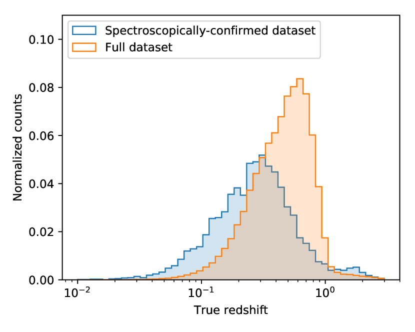
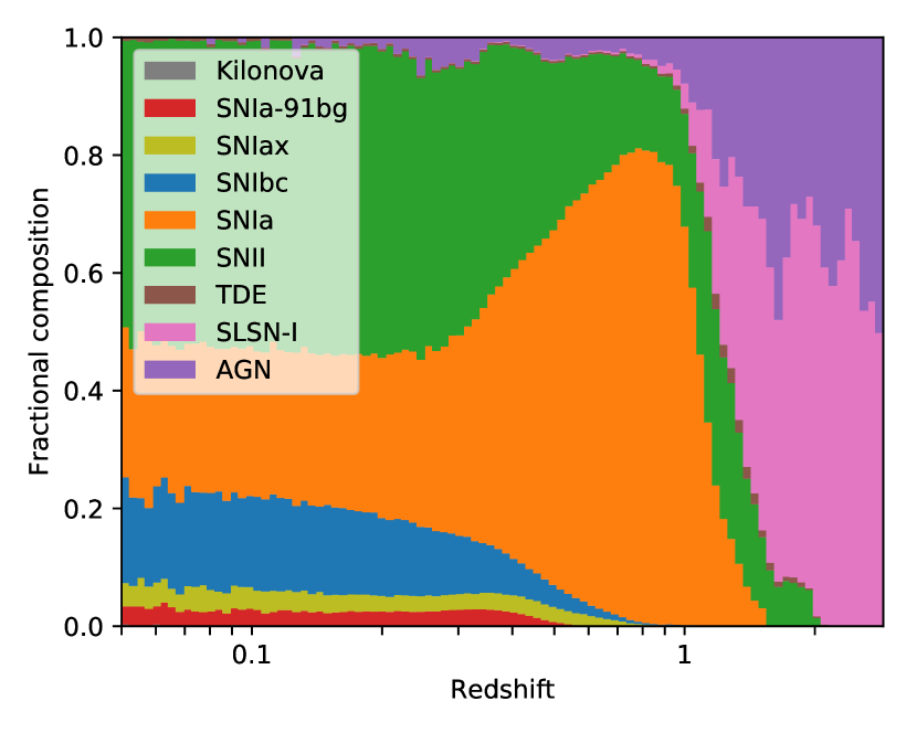
The training set for surveys such as LSST will likely be highly biased since spectra are required to categorize each object in the training set. Typical choices of followup strategies will preferentially select brighter, closer objects. For the PLAsTiCC simulations, this bias can be seen in Figure 1. The median redshift of the training set is 0.18, compared to 0.43 for the full dataset. An additional challenge is that the different transients and variables have very different redshift distributions, as illustrated in Figure 2, so the biases in the training set will not be the same across different object types.
2.2 Metrics
2.2.1 Flat-weighted metric
As discussed in Malz et al. (2018), the PLAsTiCC team proposed to evaluate the performance of different classifiers on the PLAsTiCC dataset using a weighted multi-class logarithmic loss metric:
| (1) |
where is the total number of classes and is the number of objects of each class. is 1 if the object belongs to class and 0 otherwise. are the predictions of a classifier, and for each object we should have . The class weights can be chosen to emphasize the performance of the classifier on specific classes.
An unweighted logarithmic loss is minimized when the classifier outputs predictions for each class that match the conditional probabilities of each class given the observations. By dividing by the total counts for each class, the logarithmic loss is normalized so that each class effectively has the same weight. This is important for the PLAsTiCC simulations because some classes have many more observations than others (e.g. over 10,000 SNe Ia for each kilonova), and an unweighted logarithmic loss would favor a classifier that does not attempt to classify the poorly-represented classes. For an optimal classifier trained on this metric, can be interpreted as a probability. By this, we mean that given a sample with equal number of objects from each class, 40% of the objects that are assigned will belong to class .
In our main analysis, we choose to use the metric of Equation 1 with class weights of for all of the classes present in the training set. We did not attempt to produce a classifier that can identify objects that do not have examples in the training set, so we set for all such classes (the classes with IDs starting with 99 in Table 1). We call this metric the “flat-weighted metric” because it gives all of the classes the same weights. The flat-weighted metric can be written as:
| (2) |
where the iteration over classes only considers classes that have examples in the training set, and is the number of such classes.
2.2.2 Redshift-weighted metric
For some science cases, a subtle issue with the flat-weighted metric in Equation 2 is that it does not take the redshift of extragalactic transients into account. If a classifier trained on this metric is given information about the redshifts of the different objects, the classifier will learn to use the redshift distributions of different transients in the training set to perform its classification. For example, SNe Ia tend to be discovered at higher redshifts than most other kinds of supernovae, so a classifier trained on the flat-weighted metric will tend to classify ambiguous supernovae at high-redshifts as SNe Ia, and ambiguous supernovae at lower redshifts as other kinds of supernovae. Examples of this effect for the classifiers trained in this paper will be shown in Section 4.2.
For photometric classification, classifiers are typically trained on datasets of spectroscopically-confirmed objects that have biased redshift distributions. It is the redshift distributions of these biased training sets that will be encoded into the predictions, not the redshift distributions of the test set. For a classifier trained on a metric similar to Equation 1, any analysis that depends on understanding the performance of the classifier as a function of redshift (such as cosmology with SNe Ia) requires accurate estimates of the differences between the redshift distributions in the training and full datasets. This is a difficult task if the spectroscopic followup is distributed across many different telescopes with varying observing strategies and objectives. One naive approach to dealing with this issue is to not input measurements of the redshifts of objects into the classifier, in an attempt to prevent it from using the redshifts to make its decisions. However, the redshift affects almost all features of a light curve, so a classifier can obtain a fairly accurate estimate of the redshift of an object through features such as the relative flux levels in different bands or the time dilation of the light curve, and it can use these estimated redshifts to make its predictions.
To mitigate this issue, we introduce the concept of a redshift-weighted metric. We reweight the objects in the training set so that every object class effectively has the same chosen redshift distribution. When a classifier is trained to optimize such a metric, the classifier cannot use the redshift distributions of the objects in the training sample for classification because they are all identical. We implement such a metric by splitting the redshift range into 10 logarithmically-spaced redshift bins between redshifts 0.1 and 3, along with an additional bin for Galactic objects for a total of 11 redshift bins. We then assign weights to each object to normalize the number of objects of each class in each redshift bin. This results in the following redshift-weighted metric:
| Redshift- | ||||
| (3) |
Here, is 1 if object belongs to class and is in redshift bin . is the total number of redshift bins. is the total number of objects in class and redshift bin . To avoid extremely large weights for objects in bins that have very few counts, we impose a floor on of 100 objects. For extragalactic objects, we choose to set the weight to . A typical extragalactic class is well-represented in roughly half of the different redshift bins while Galactic objects only have a single bin. To roughly maintain a flat class weighting, we set the weight for Galactic objects to the average number of bins that are well-populated for extragalactic classes (5). As for the flat-weighted metric, we set for the objects that were not present in the training set since we did not attempt to classify them.
2.2.3 Kaggle metric
For the blinded phase of the PLAsTiCC hosted on Kaggle, the performance of classifiers was evaluated using the “Kaggle metric” which is of the weighted multiclass logarithmic-loss metric in Equation 1 with the class weights shown in Table 1. One part of the blinded phase of the PLAsTiCC was identifying new kinds of objects that had no examples in the training set (the “class 99” objects). In this work, we did not attempt to address this part of the challenge. Use of the Kaggle metric requires values for the class 99 objects. Hence, to evaluate the performance of our classifiers on the Kaggle metric, we generate artificial predictions for the class 99 objects using formulae that were tuned by probing the metric during the blinded phase of the PLAsTiCC. For Galactic objects, we assign a flat predicted probability of 4% to the class 99 objects. For each extragalactic object, we assign a predicted probability according to the following formula:
| (4) |
where is the predicted probability assigned to the class with ID (see Table 1 for the list of IDs). We then rescale all of the predicted probabilities so that they sum to 1 for each object. Note that these formulae are not a proper way of identifying new objects in the data. All of the top 5 performing teams in the blinded phase of the PLAsTiCC used similar formulae, and we are not aware of any successful attempts to identify new objects. For the analyses in this paper, we primarily use the flat-weighted metric and redshift-weighted metric, which both ignore the class 99 objects. We do however evaluate our performance on the Kaggle metric using these formulae for the class 99 predictions for comparison purposes.
2.2.4 Single class metrics
Finally, we evaluate several standard metrics for the performance of a deterministic classifier when identifying objects of a single specific type. The confusion matrix and corresponding labels for each of the outcomes of classification of one transient type out of a larger sample are shown in Table 2. Using the labels from this table, we define the following metrics that will be used in further analysis:
| (5) |
| (6) |
| (7) |
| (8) |
| True Class | |||
|---|---|---|---|
| P | N | ||
| Predicted | P | True positive (TP) | False positive (FP) |
| Class | N | False negative (FN) | True negative (TN) |
We also calculate the Area under the Receiver Operator Characteristic Curve (AUC) for each of our classes. This metric is defined as the area under the curve of the TPR plotted against the FPR, and ranges between 0.5 for a random classifier to 1 for a perfect classifier. See L16 for more complete definitions of all of these metrics.
3 Methods
3.1 Overview
Our approach to photometric classification combines several techniques. We first preprocess the light curves as described in section 3.2. In Section 3.3, we describe how we use Gaussian process (GP) regression to predict smooth models for each of our sparsely sampled light curves. Using these GP models, as discussed in Section 3.4, we augment the spectroscopically-confirmed dataset, generating artificial light curves that are more representative of the full dataset. In Section 3.5, we describe how for each light curve in the augmented training set, we calculate a set of features from the GP models. We then train a tree-based classifier on the extracted features to perform the final classification predictions, the details of which can be found in Section 3.6.
3.2 Light curve preprocessing
The fluxes of transients are typically determined by subtracting newly measured fluxes from fluxes measured from a set of reference images. For long-lived transients, these reference images may contain light from the transients themselves. The blinded PLAsTiCC dataset did not provide the reference fluxes of the sources, so for objects such as variable stars, the “background” level of the light curve is simply the flux of the light curve at an arbitrary point in time. To address this issue, we estimate new “background” levels for each light curve using a biweight estimator (Beers et al., 1990). For short-lived transients, this background estimator will return the flux level at times when there is no light from the transient. For sources such as variable stars or active galactic nuclei, this robust estimator will effectively return the mean value of the light curve.
3.3 Modeling light curves with Gaussian process regression
Gaussian process (GP) regression has been shown to be effective for several applications of astronomical light curve modeling. Kim et al. (2013) used GPs to model the light curves of SNe Ia and predict their peak brightnesses. Fakhouri et al. (2015) and Saunders et al. (2018) modeled the full spectral time-series of SNe Ia with GPs, and used these models to evaluate the spectra of these objects at arbitrary times. L16 introduced GP modeling for astronomical transient classification. R18 showed that GP models can be used to augment a biased training set by generating additional training data from the GPs. These works all focused specifically on using GPs to model particular kinds of supernovae. We extend these techniques so that they can be applied to a wider range of transients and variables. An introduction to GP regression can be found in Appendix A.
Previous works using GPs for photometric classification (e.g. L16 and R18) evaluated separate GPs for each band of the light curve, so the model was not able to take cross-band information into account. In contrast, in this work, we use GPs in both time and wavelength to model the light curve in all bands simultaneously. We do not attempt to explicitly model the throughputs of the different filters. Instead, we calculate central wavelengths for each of the bands using the estimated LSST throughputs333https://github.com/lsst/throughputs assuming a source with a constant spectrum. We use these central wavelengths as the coordinates for the wavelength dimension of the GP. This effectively means that the GP is producing a model of the spectrum convolved with a broad filter rather than modeling the spectrum directly.
We use the George package (Ambikasaran et al., 2015) to implement our GPs. Using maximum likelihood estimation, we fit for both the amplitude () and time length scale () parameters on a per-object basis. It is difficult to reliably fit the length scale in wavelength on a per-object basis due to the fact that there are only 6 filters used for observations. We choose to fix the length scale in wavelength to 6000Å because we find that this value produces reasonable models for all of the transients and variables in the PLAsTiCC dataset. The results of this analysis are not highly sensitive to the choice of the length scale in wavelength.
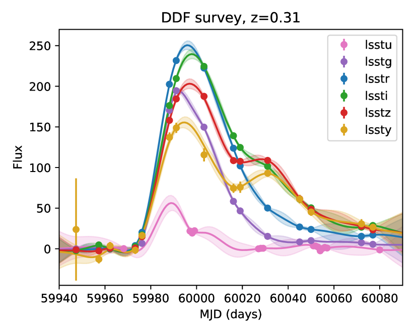
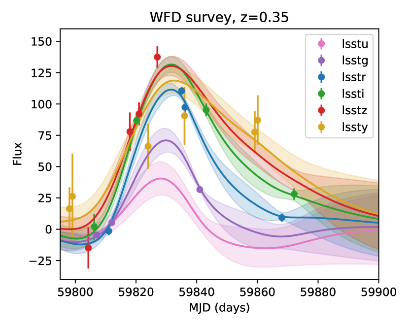
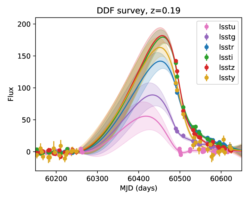
Examples of the GP model for a well-sampled SN Ia light curve and a poorly sampled one are shown in Figure 3. The GP produces reasonable non-parametric models of the light curves that can be used for further analysis, along with estimates of the model uncertainties. Because we are using a kernel in both wavelength and time, the GP is able to use cross-band information to infer the supernova light curve even in bands where there are few observations. This can be seen in the right plot of Figure 3 where the GP produces a reasonable model (with high uncertainty) of the light curve in the LSST band even though there are no observations in this band.
3.4 Augmenting the training dataset
The spectroscopically-classified objects that are used as a training set for photometric classifiers tend to be highly non-representative of the full dataset in terms of their redshift and signal-to-noise distributions. These training sets are typically strongly biased towards bright, low-redshift objects. Most previous attempts at producing photometric classifiers have seen strongly degraded performance when trained on non-representative datasets, and have concluded that obtaining representative training sets is essential for photometric classification (e.g. L16). More recently, R18 showed that it is possible to apply various transformations to the light curves in the original training set to generate a new training set that is more representative of the test set. We call this process “augmentation” of the training set. Using their STACCATO framework for augmentation, R18 train a classifier whose performance is significantly better (AUC of 0.96 on the SNPhotCC dataset) than one trained on the original non-representative training set (AUC of 0.93), and approaching the performance of a classifier trained on a representative training set (AUC of 0.977).
In STACCATO, GPs are fit to the observations of each object in the training set, with separate GPs for each band. “Synthetic light curves” are then produced for each object by sampling from the GPs. Each sample from a GP produces a different continuous function that can be interpreted as a synthetic light curve that is consistent with the observations of the original object. By repeatedly sampling from the GPs, many synthetic light curves can be produced for each object in the training set. In STACCATO, for every object, a “propensity score” is calculated, which is an estimate of how likely the object is to make it into the training set. The propensity score is then used to determine how many different synthetic light curves to make for each object in the training set. By generating different number of synthetic light curves for each object in the training set, an “augmented” training set of synthetic light curves is produced that is more representative of the test set. Finally, a classifier is trained on the set of synthetic light curves.
Our approach to augmentation differs in several ways from the approach of R18. In STACCATO, different synthetic light curves are generated for each object, but these synthetic light curves all use the same set of observations. Instead, our augmentation procedure involves simulating entirely new sets of observations for each object. When augmenting a light curve from the training set, we throw out large blocks of observations to simulate season boundaries, take originally well-sampled light curves and degrade their sampling, and add noise to the light curve in different bands. We measure the cadence and depth of observations in the test set, and generate augmented light curves that have similar cadences and depths of observations to the test set. This ensures that the light curves in the augmented training set have observations that are representative of the observations of light curves in the test set regardless of the light curve quality in the original training set. We also interpret the GP uncertainty as an uncertainty due to poor measurement rather than intrinsic variation of the light curve. For this reason, we choose to use the mean prediction of the GP for our augmented light curves, and we propagate the GP prediction uncertainties into the uncertainties of the generated observations.
Additionally, we introduce the concept of “redshift augmentation” where we take an object in the training set and simulate observations of it at different redshifts. Because we are using a Gaussian process in both time and wavelength, we can shift the redshift of an object by evaluating the Gaussian process predictions for the light curve of that object at the redshifted wavelengths. Note that the GP is effectively modeling the spectrum of the object convolved with a filter. Assuming that this convolved spectrum is reasonably smooth and that the different filters have similar profiles, the two-dimensional GP predictions will automatically include k-corrections (Oke & Sandage, 1968) to the observed brightnesses in each filter. There will be higher-order corrections due to sharp structure in the spectrum (e.g. emission lines) and differences in the filter shape, but these are unlikely to significantly affect the classification in most cases. When redshifting the observations of an object, we then update the observed brightnesses by calculating the difference in distance modulus assuming a fiducial cosmology. After these procedures, we have effectively simulated the light curve for an object at a different redshift than it was originally observed at.
With redshift augmentation, if we observe an object at one redshift, then we can effectively use that object for training at all redshifts. Because training samples are typically biased towards bright, low-redshift objects, this means that we can use redshift augmentation to fill in the missing regions of parameter space in the training sample at high redshifts. This differs from the augmentation procedure in STACCATO. While STACCATO is making additional versions of light curves for objects that were already at high redshifts, we are instead taking low-redshift light curves and simulating what they would look like if they had been observed at high redshifts. A potential caveat with redshift augmentation is that the subpopulations of different object types could evolve with redshift. We discuss how this this can be addressed in Section 5.3.
One major challenge with augmentation is determining where in parameter space to generate new objects to match the training set to the test set. STACCATO uses a “propensity score” to decide how many new versions should be generated for each object in the training set. Unfortunately, for this technique to be effective, the rates and selection efficiencies in the test set must be known for each object type. The rates of different transients are not currently well known in many regions of parameter space. For SNe Ia and core-collapse supernovae, the current best measurements of the rates above redshift 1 have uncertainties of roughly 50% of the measured rates (e.g. Okumura et al. (2014); Rodney et al. (2014); Strolger et al. (2015)). To address this issue, we instead choose to design a classifier whose performance is independent of the rates and selection efficiencies in the training set. This can be done by training a classifier to optimize the metric described in Section 2.2.2; a discussion of the effectiveness of this procedure will be shown in Section 4.2. When training a classifier with these properties, for the augmentation procedure, we simply need to ensure that we generate a set of light curves covering the full parameter space for any object type at a given redshift. We therefore simulate each object in our training set the same number of times at a range of different redshifts.
The full details of our augmentation procedure can be found in Appendix B. A summary of our approach to augmentation is as follows:
-
1.
Fit a GP to a light curve in the original training sample to use as a template.
-
2.
Choose a new redshift for extragalactic objects, or brightness for Galactic objects.
-
3.
Evaluate the mean GP prediction and uncertainty to obtain a new light curve at the chosen brightness/redshift.
-
4.
Drop observations to simulate poorly-sampled light curves from the well-sampled training light curves.
-
5.
Add measurement uncertainties that are representative of the test dataset.
-
6.
Ensure that the generated light curve would be detected.
-
7.
Simulate a photometric redshift following the mapping between spectroscopic and photometric redshifts in the test dataset.
-
8.
Repeat these steps until a large enough augmented sample has been obtained.
For this analysis, we use the same augmented training set to train all of the different classifiers that will be discussed. We generate up to 100 different versions of each light curve in the training set, which results in a total of 591,410 light curves in the augmented training set.
3.5 Extracting features from the light curves
To extract features from a light curve, we begin by performing a GP fit as described in Section 3.3 and computing the mean GP flux predictions in the LSST , , and bands. We choose to use the observer-frame LSST band as the reference for many of our features because this band typically has a reasonable flux level for both the low and high-redshift objects in our sample. We extract a variety of features from the GP flux predictions in each of these three bands, the details of which can be found in Table 3.
| Feature name | Description |
|---|---|
| host_photoz | Host-galaxy photometric redshift, taken directly from the PLAsTiCC metadata. |
| host_photoz_err | Host-galaxy photometric redshift error, taken directly from the PLAsTiCC metadata. |
| length_scale | Fitted GP length scale hyperparameter, in days. |
| max_mag | Peak magnitude of the GP flux prediction in the LSST band. |
| pos_flux_ratio | Ratio of the maximum positive flux to the maximum-minus-minimum flux in the LSST band. |
| [max,min]_flux_ratio _[blue,red] | Normalized difference of the light curve colors at maximum/minimum light. The blue measurement is the difference between the LSST and bands, and the red measurement is the difference between the LSST and bands. The normalized difference is calculated by taking the difference of the fluxes in the two bands divided by their sum. |
| max_dt | Difference of the time of maximum in the LSST and bands in days. |
| [positive,negative] _width | An estimate of the light curve “width” that is applicable even for non-supernova-like transients and variables. This is implemented as the integral of the positive/negative parts of the GP flux predictions divided by the positive/negative maximum fluxes. |
| time_[fwd,bwd]_max _[0.2,0.5] | Measurements of the rise and decline times of a light curve. This measurement is defined as the time in days for the light curve to rise (bwd) or decline (fwd) to a given fraction (either 20% or 50%) of maximum light in the LSST band. |
| time_[fwd,bwd]_max _[0.2,0.5]_ratio _[blue,red] | Ratio of the rise/decline times calculated as described above in different bands. The blue measurement is the difference between the LSST and bands, and the red measurement is the difference between the LSST and bands. |
| frac_s2n_[5,-5] | Fraction of observations that have a signal greater than 5/less than -5 times the noise level. |
| frac_background | Fraction of observations that have an absolute signal-to-noise less than 3. |
| time_width_s2n_5 | Time difference in days between the first observation with a signal-to-noise greater than 5 and the last such observation (in any band). |
| count_max_center | Number of observations in any band within 5 days of maximum light. |
| count_max_rise _[20,50,100] | Number of observations in any band between 20, 50, or 100 days before maximum light and 5 days after maximum light. |
| count_max_fall _[20,50,100] | Number of observations in any band between 5 days before maximum light and 20, 50, or 100 days after maximum light. |
| peak_frac_2 | Ratio of the maximum flux in the second most prominent peak in the light curve to the maximum flux in the main peak, averaged over all LSST bands. This is intended to identify supernova-like objects that only have a single large peak in most bands. |
| total_s2n | Total signal-to-noise of all observations of the object. |
| percentile_diff _[10,30,70,90]_50 | Measurements of the distributions of the observed fluxes. For each band, we calculate the flux level for a given percentile of observations, and normalize it by the maximum-minus-minimum of the GP flux predictions. We then take differences between this measurement for various percentiles and the percentile measurement. The final value is the median of the calculated differences in all bands. |
In general, we find that in the PLAsTiCC dataset, the non-supernova-like variables and transients end up being relatively easy to distinguish, so most our our effort went to identifying features that are effective for distinguishing the different kinds of supernovae. We initially generated hundreds of different features, and we used both the feature importance ranking of our classifier and cross-validation performance (discussed in Section 3.6) to select a subset of 41 features that give good performance. Most of the features that we include are standard features that are well-known to distinguish transients, such as the apparent peak brightness of the transient and the photometric redshift. We include measures of the colors of the objects by taking ratios of the peak brightnesses in different bands, and estimates of the rise time and fall times that help distinguish between the different supernova types.
One major difference between this analysis and most previous ones is that our light curve model includes cross-band information. The GP flux predictions in a given band incorporate information from nearby bands because of the GP kernel in the wavelength direction. We only calculate features from the GP predictions in the LSST-, , and bands, but these features capture the observations in all of the different bands. This can be seen for the poorly-sampled light curve in Figure 3 where we have reasonable models of the light curve even in bands with no observations. We find that calculating features off of GP flux predictions in additional bands beyond the three previously listed does not improve the classification for the PLAsTiCC sample. This kind of analysis is only possible with a light curve model that fits both wavelength and time directions simultaneously as opposed to traditional models where each band is fit independently. Although we chose to perform the GP flux predictions at the wavelengths associated with several LSST bands for simplicity, the GP flux predictions can be performed at arbitrary wavelengths, and observations from different bands or other telescopes can easily be included in the GP model.
There are a handful of notable features that we introduced that have not been included in previous analyses. First, we add several features that are effective at classifying variable object types, most notably the percentile_diff_X_Y features that measure the distribution of the photometry values. These features are effective at distinguishing object types with large wings in their photometry distributions (e.g. eclipsing binaries) from object types that have more even distributions (e.g. Mira variables), even with relatively few observations.
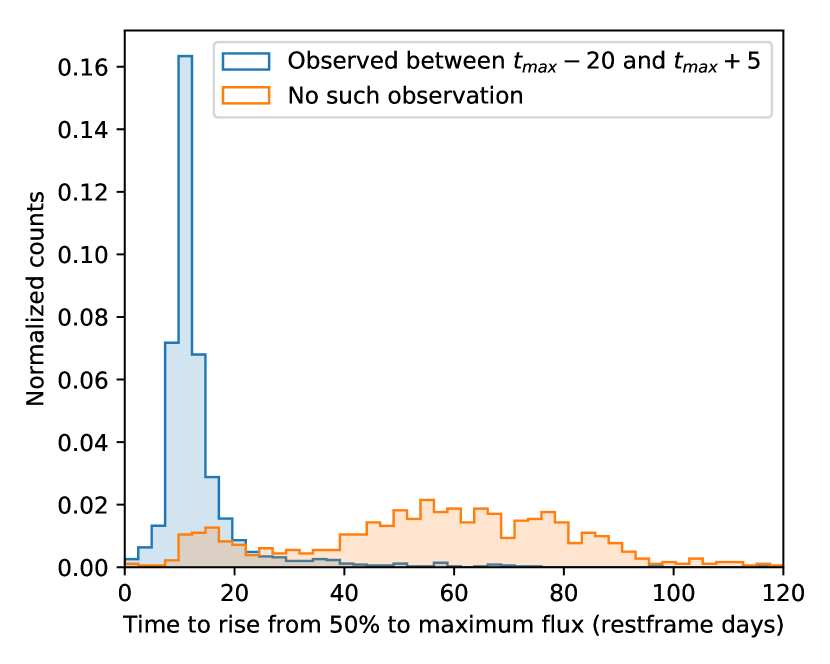
Another novel technique in this work is the introduction of features that measure the fit quality. In many cases, the available photometry for an object does not cover its full light curve. An example of such a light curve for a Type Ia supernova can be seen in Figure 4. Without any photometry before maximum light, the GP produces a model with large uncertainties, and the measurement of the rise time will be both uncertain and biased. We experimented with several approaches to incorporating this information into the classifier, and found that measuring the number of observations in various bands around maximum light provides an excellent way to evaluate the accuracy of the rise time measurements. The right panel of Figure 4 illustrates this for SNe Ia: light curves that have an observation between 20 observer-frame days before maximum light and 5 days after maximum light have a tight distribution of measured rise times, while light curves without this information have a wide, biased distribution of rise times. By adding features measuring the number of observations in various time intervals, the classifier can effectively determine how reliable other features, such as the rise time information, are.
3.6 Training a LightGBM model
We train a gradient boosted decision tree classifier on features extracted from the augmented training set. Decision trees are a classification technique where objects are filtered through a variety of cuts to attempt to separate them into their different classes. Boosted decision trees combine a large number of these trees to produce a robust classifier, and have proven to be very effective at a variety of different classification tasks in astronomy (e.g: Bailey et al. (2007), L16). Using the LightGBM implementation of gradient boosted decision trees (Ke et al., 2017), we train separate classifiers to optimize objective functions that are direct implementations of the metrics in Equations 1 and 2.2.2.
To evaluate and optimize the performance of the classifier, we use five-fold cross-validation on the augmented training set. We partition the augmented training data into five separate subsets that each have equal ratios of the different targets. We then train five separate classifiers, each of which is trained on four of the five subsets, and we evaluate its performance on the remaining subset. By repeating this procedure for each of the subsets, we obtain out-of-sample predictions for every object in the augmented training set. We then evaluate the PLAsTiCC metric on these predictions, and use this cross-validation performance to tune our model. For the augmented dataset, we ensure that all light curves generated from the same original light curve are included in the same subset to avoid leaking information across the subset boundaries. When generating predictions for objects that are in the test set, we evaluate the average of the classification probabilities for the new objects from each of the five trained classifiers.
We optimize the hyperparameter values of the LightGBM model by scanning over each hyperparameter individually and evaluating the cross-validation performance on the flat-weighted metric. The resulting hyperparameter values are shown in Table 4. The optimal hyperparameter values are relatively stable across different sets of features and target metrics, so for simplicity we use the same hyperparameter values for all of the analysis variants.
| Hyperparameter name | Value |
|---|---|
| boosting_type | gbdt |
| learning_rate | multi_logloss |
| colsample_bytree | 0.05 |
| reg_alpha | 0 |
| reg_lambda | 0 |
| min_split_gain | 10 |
| min_child_weight | 2000 |
| max_depth | 7 |
| num_leaves | 50 |
| early_stopping_rounds | 50 |
We train two separate versions of our classifier, one of which is optimized for performance on the flat-weighted metric defined in Equation 2, and one of which is optimized for performance on the redshift-weighted metric defined in Equation 2.2.2. Both of these classifiers are trained on the same augmented training set. For the training set, the Kaggle metric is nearly identical to the flat-weighted metric, so we do not train a separate classifier to optimize it.
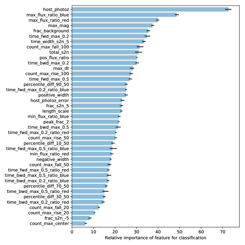
LightGBM outputs a measure of how much each feature contributed to the classification. We call this measure the “importance” of that feature for classification. The importance of each feature for a classifier trained to optimize the flat-weighted metric are shown in Figure 5. The most important features for classification are the photometric redshift of the host galaxy, the peak brightness, and the colors of the light curves at maximum light. The feature importance plot for a classifier trained to optimize the redshift-weighted metric looks nearly identical.
4 Results
4.1 Overall performance
The results of both of our classifiers for many of the metrics defined in 2.2 are shown in Table 5. In general, we find that both classifiers have similar performance across all of these global metrics. In the blinded phase of the PLAsTiCC, an earlier version of our algorithm won the challenge with a score of 0.680 on the Kaggle metric (lower is better). The updated algorithm presented in this paper achieves a slightly better score of 0.649 on this metric. This improvement mainly came from restricting the allowable redshift range for the data augmentation procedure and propagating uncertainties. Our original augmentation algorithm was allowed to modify the redshifts of objects arbitrarily. At high redshifts, unreliable extrapolations of the GP models far into the restframe UV were being used to produce the light curves. Additionally, we were not propagating the GP modeling uncertainties into the generated fluxes. These issues were fixed for the version of the algorithm described in this paper which dramatically improved performance at high redshifts.
| Metric name | Flat-weighted classifier | Redshift-weighted classifier |
|---|---|---|
| Flat-weighted metric | 0.468 | 0.510 |
| Redshift-weighted metric | 0.523 | 0.500 |
| Kaggle metric | 0.649 | 0.709 |
| AUC – 90: Type Ia SN | 0.95721 | 0.95204 |
| AUC – 67: Peculiar Type Ia SN – 91bg-like | 0.96672 | 0.96015 |
| AUC – 52: Peculiar Type Ia SN – SNIax | 0.85988 | 0.84203 |
| AUC – 42: Type II SN | 0.93570 | 0.90826 |
| AUC – 62: Type Ibc SN | 0.92851 | 0.91558 |
| AUC – 95: Superluminous SN (Magnetar model) | 0.99442 | 0.99257 |
| AUC – 15: Tidal disruption event | 0.99254 | 0.99243 |
| AUC – 64: Kilonova | 0.99815 | 0.99579 |
| AUC – 88: Active galactic nuclei | 0.99772 | 0.99706 |
| AUC – 92: RR Lyrae | 0.99987 | 0.99986 |
| AUC – 65: M-dwarf stellar flare | 0.99999 | 0.99999 |
| AUC – 16: Eclipsing binary stars | 0.99983 | 0.99983 |
| AUC – 53: Mira variables | 0.99947 | 0.99937 |
| AUC – 6: Microlens from single lens | 0.99962 | 0.99966 |
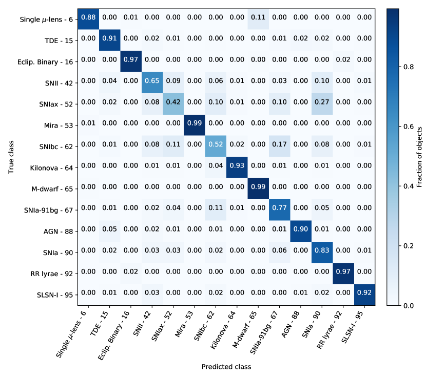
Figure 6 shows a confusion matrix for the flat-weighted classifier which can be used to evaluate its performance on specific classes. For most classes, the top prediction of this classifier is correct with an accuracy over over 80%. The main challenge for the classifier is distinguishing between the different types of supernovae. For example, Type Iax supernovae are misclassified as Type Ia supernovae 27% of the time, and Type Ibc supernovae are misclassified as Type Ia-91bg supernovae 17% of the time. This misclassification is often highly asymmetrical: only 3% of Type Ia supernovae are misclassified as Type Iax supernovae. This is likely due to the fact that the training set of Type Iax supernovae (183 objects) is small compared to the sample of Type Ia supernovae (2,313 objects), and there is additional diversity in the test set that is not seen in this small training set of Type Iax supernovae. Methods to address these differences will be discussed in Section 5.2. The redshift-weighted classifier has a confusion matrix that is nearly identical to the one for the flat-weighted classifier. Note that the confusion matrix only considers the top prediction for each object while our classifier outputs a probability for each object type, meaning that there is additional information available for further analyses that is not captured by the confusion matrix.
4.2 Redshift-dependent performance
Despite the similarity in performance between the flat-weighted classifier and redshift-weighted classifier on most global metrics, they exhibit very different performance as a function of redshift. For a fixed overall sample purity of 95%, we calculate the completeness of the SN Ia sample as a function of redshift. The results of this procedure can be seen in Figure 7.
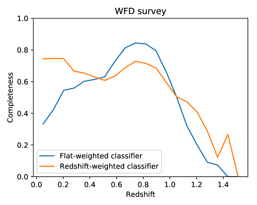
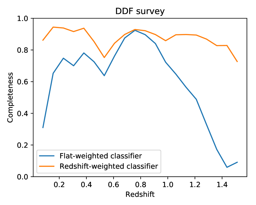
We find that the performance of the flat-weighted classifier has undesirable behavior as a function of redshift. For objects observed in the WFD survey, we find that this classifier has its peak completeness at redshift 0.8 where it correctly classifies 80% of the SNe Ia. At nearby redshifts, its completeness drops to below 40%. The reason for this strange performance can be seen in Figure 2. Around redshift 0.8, nearly 70% of the observed objects are Type Ia supernovae, so the flat-weighted classifier is using information about the redshift distributions of the different transients at different redshifts as part of its classification. Only 0.6% of the SNe Ia in the sample are at a redshift less than 0.1, so the flat-weighted classifier infers that any object at those redshifts is likely not to be a SN Ia, and therefore has a very poor completeness for low-redshift SNe Ia. We see similar effects for the DDF survey.
Any classifier trained to optimize traditional metrics on a biased training sample will run into these issues if it is allowed to incorporate redshift information into its predictions. Furthermore, the classifier is learning to use the redshift distributions of objects in the training set, not the redshift distributions of ones in the test set. As described in Section 3.4, we expect there to be large discrepancies in the redshift distributions of these two sets, even for augmented training sets. A classifier trained on the redshift-weighted metric provides a solution to this problem by outputing a probability for each object type assuming that each class has the same arbitrarily chosen redshift distribution in the training set. The performance of such a classifier will not depend on the redshift distributions of the different kinds of objects in the training set. This can be seen in Figure 7: for the WFD survey, the redshift-weighted classifier shows a stable completeness of 70% at low redshifts, and its completeness declines nearly monotonically at higher redshifts as the signal-to-noise decreases. The redshift-weighted classifier is able to classify objects in the DDF survey with a completeness of above 80% at most redshifts, maintaining this performance for even the highest-redshift SNe Ia in the test sample at z=1.55.
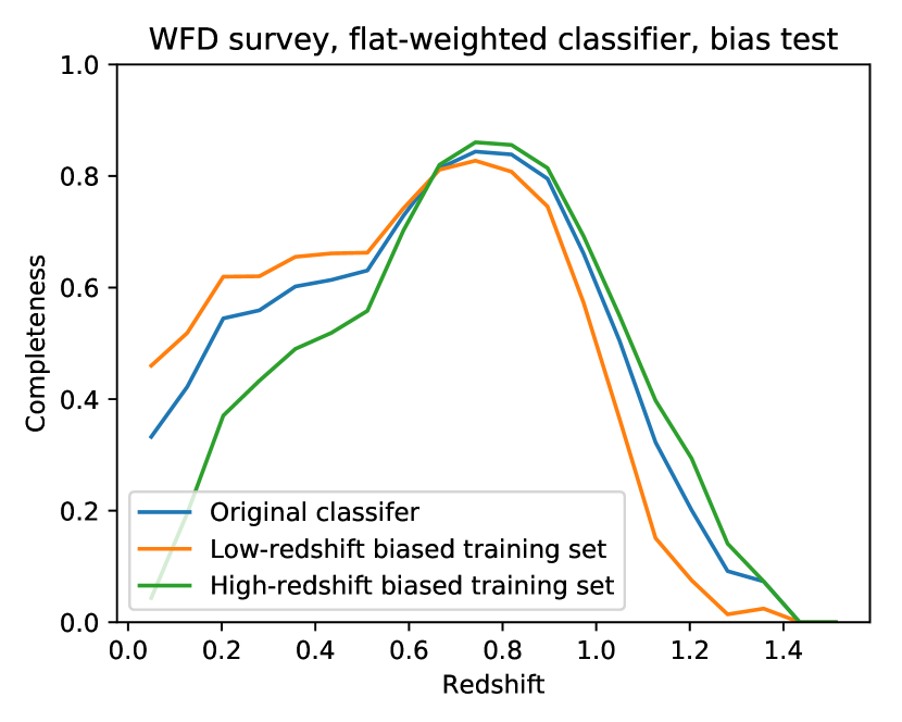
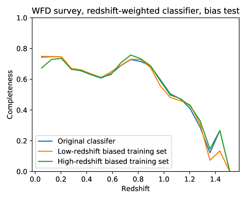
To validate the claim that the classifications produced by a classifier trained on the redshift-weighted metric are independent of the redshift distributions of objects in the training set, we simulated modifying the redshift distribution of the SNe Ia in the training set. Starting with the same augmented training set used to train the original classifiers, we create a low-redshift-biased training set by randomly dropping light curves of SNe Ia from the training set with probability . Similarly, we create a high-redshift-biased training set by randomly dropping light curves of SNe Ia from the training set with probability . We keep all light curves from the transients that are not SNe Ia so that only the redshift distribution of SNe Ia is changing between the original augmented training set and the biased training sets. We then retrain our flat-weighted and redshift-weighted classifiers on these new training sets. The results of this procedure can be seen in Figure 8. For the flat-weighted classifier, the classifier performance varies dramatically for these different training sets. At low and high redshifts, the difference in completeness between the different classifiers varies by more than a factor of two. For the redshift-weighted classifier, however, the different classifiers have nearly identical completenesses as a function of redshift. Only small deviations from the original performance are seen at the very edges of the redshift range where we have thrown out almost all of the SNe Ia in the biased training sets.
4.3 Comparison to other models
A full comparison of our classifier to all of the other classifiers submitted to the blinded phase of the PLAsTiCC will be presented in Hložek et al. (2019, in prep.). Those classifiers used a wide range of techniques that were not explored in this paper, including template fitting, recurrent neural networks and denoising autoencoders. However, all of those models were trained to optimize the Kaggle metric, and we find that they exhibit the same problematic performance with redshift as discussed for our flat-weighted classifier in Section 4.2. The classifiers presented in this paper are currently the best-performing models on the PLAsTiCC dataset, scoring 0.468 on the flat-weighted metric compared to 0.481 for the next-best model submitted to the blinded phase of the PLAsTiCC challenge. On the redshift-weighted metric, our redshift-weighted classifier scores 0.500, significantly better than the next-best model which scores 0.609. Our classifier can therefore serve as a benchmark for future photometric classifiers.
5 Discussion
5.1 Computing resources
The main limitation on computing speed for this model is the GP regression. We perform our computation on an Intel Xeon E3-1270 v3 CPU. A single core on this machine can fit the GP hyperparameters and extract features for 10 objects per second. Training the LightGBM classifier takes 30 minutes for an augmented training set of 591,410 objects after the features have been computed. Generating predictions with the trained classifier takes a negligible amount of time compared to feature extraction (1000 objects per second). Processing the entire PLAsTiCC dataset therefore takes 100 core hours of computing time.
Predictions from this classifier can easily be done in real time. A machine with 100 CPU cores similar to the one used for our testing could process 1000 objects per second and provide live typing estimates for all of the transients and variables discovered in a survey. As new spectroscopic confirmations of objects are obtained, the classifier could periodically be retrained to incorporate that new data into its training set. The GP fits and feature extractions do not need to be redone for older data so long as the feature extraction algorithm is unchanged, so retraining the classifier on new data can be done in under an hour in most cases.
5.2 Representativeness of the augmented training set
Ideally, our data augmentation procedure would produce an augmented training set that is fully representative of the test set. In practice, however, there are several reasons why an augmented training set may differ from the test set. First, the training set must cover the full intrinsic diversity of objects of the test set. Note that the augmentation procedure does not attempt to simulate new objects, it simply produces light curves for previously-measured objects under different observing conditions and at different redshifts. If there are rare subtypes of objects that only appear in the test set (e.g. peculiar supernovae), and that have very different light curves from the objects in the training set, then the augmentation procedure will not be able to produce light curves that are similar to the ones observed for these objects. This issue can be addressed by using active learning when obtaining the training set used for classification, as described in Ishida et al. (2019). In this procedure, the output of the classifier is used to determine which objects should be targeted for spectroscopic followup. This helps to ensure that the original training set contains examples of all of the different object types that are present in the full dataset.
The second major challenge for representativeness is in handling the different redshift distributions for object types between the training and test sets. As discussed in Section 3.4, the rates of different transients are not currently known well enough as a function of redshift to produce an augmented dataset that is truly representative of the test dataset. Instead, by training a classifier on a redshift-weighted metric, we obtain a classifier whose output is independent of the redshift distributions of the classes in the training sample, as shown in Section 4.2. Such a classifier effectively produces classification probabilities assuming the same arbitrarily chosen redshift distribution for every class. In our implementation, we are using a log-uniform distribution in redshift for our classification, and this assumed distribution can easily be propagated to further analyses. Analyses that depend on photometric classification, such as cosmology with SNe Ia, are already typically required to fit for or model the rates and selection efficiencies of different transient types as a function of redshift to achieve their science goals. A redshift-weighted classifier produces output classification probabilities that depend on known redshift distributions, and the biased redshift distributions in the original training set will have no effect on the classification probabilities.
Our redshift-dependent classifier specifically addressed the issue of having different redshift distributions between the training and test sets. A similar procedure could be applied to other observables of the transients, including but not limited to their peak brightnesses, host properties, or rise and fall times. Assuming that these properties can be measured accurately enough in the training set, we can simply reweight objects in the training set to force the classifier to assume the same arbitrarily chosen distribution over this observable for each object type. This effectively means that the classifier cannot learn anything from the distribution of this observable, or any indirect measurements of the distribution of this observable to classify objects. The observable only needs to be available for the training set, and does not necessarily need to be a feature that is used for classification. For example, our redshift-weighted classifier is reweighted using the spectroscopic host redshifts of the objects in our training sample, but spectroscopic host redshifts are not available for most objects in the full dataset. Nevertheless, the classifier outputs probabilities that are independent of the distributions of spectroscopic host redshifts for different object types in the full dataset.
5.3 Handling drifting subpopulations with redshift
One potential issue with any kind of photometric classification, including redshift augmentation, is drift in the subpopulations of different types of transients as a function of redshift. For example, the properties of SNe Ia are correlated with the properties of their host galaxies such as host mass (Kelly et al., 2010). As galaxy properties evolve with redshift, the distributions of different subpopulations of SNe Ia also evolve with redshift (Rigault et al., 2013). If the spectroscopically-confirmed training set is biased to low redshifts, then a redshift-augmented training sample will have a different subpopulation distribution than the true one at high redshifts leading to a bias in the classification probabilities. This is a challenge for any photometric classification method, not just ones that use redshift augmentation, because the high-redshift followup strategy itself could be biased towards some subpopulation.
If the subpopulations of an object type can be identified in the training set using some observable, then we can reweight the training set as described previously to produce a classification assuming an arbitrarily chosen distribution over this observable, with the same assumed distribution for all object types in the sample. For instance, a dedicated campaign to measure the host masses of every galaxy in the training set could be used to produce a photometric classifier that classifies SNe Ia without taking the host mass distributions, or any indirect measurements of the host mass distributions, into account. This classifier will therefore produce classification probabilities that are independent of the change in subpopulations as a function of redshift associated with host mass. Note that this procedure could introduce biases if the observable is not available for all objects in the training sample, e.g. if it were not possible to reliably determine the host masses for higher redshift objects in the training sample.
A final concern about changing subpopulations would be if new subpopulations appear at high redshifts that are not present at low redshifts. While the survey is running, active learning, as described in Ishida et al. (2019) can be used to attempt to identify these subpopulations and trigger spectroscopic followup to add them to the training set. If, however, these new subpopulations are missed entirely in the training set, then the classifier is unlikely to be able to accurately classify objects from them.
Specific science applications may be more or less sensitive to the evolution of subpopulations with redshift. For cosmology with SNe Ia, for example, if a new subtype of SN Ia appeared at high redshift that wasn’t identified at low redshift, then it could significantly bias the cosmological analysis. This is an issue regardless of the analysis strategy: at high redshifts, a “representative sample” will likely only be able to spectroscopically type a small number of objects, potentially missing new subpopulations. A lower-redshift followup strategy that intends to use redshift-augmentation may be able to obtain a larger and more complete sample at the lower redshift, but it relies on the assumption that we can produce a reasonable model of the differences between the low and high-redshift samples. In practice, there is a trade-off between all of these concerns, and a variety of different followup strategies should be simulated to determine the optimal strategy for the science objectives.
5.4 Implications for future surveys
The results of this paper have several implications for future surveys. For surveys with limited spectroscopic resources devoted to obtaining training samples for photometric classification, previous work (e.g. L16) has suggested that these surveys should attempt to produce a training set of objects with spectroscopically-confirmed types that is as representative of the full dataset as possible. With our augmentation technique, we instead suggest that spectroscopic resources may better be used to obtain spectroscopic classifications of as many intermediate-redshift well-sampled light curves as possible. We can then use these well-sampled light curves to simulate high-redshift light curves rather than having to spend large amounts of spectroscopic followup to type high-redshift objects directly.
With augmentation, a light curve is most valuable if it has good-quality observations with a high cadence. While the labels for all of the objects in the test set that the classifier will be applied to are not known, we do know the cadence, observation depths, whether or not the light curve was impacted by season boundaries, etc. of every object in the test set. A well sampled light curve can always be degraded to simulate all of these effects, as shown in our augmentation procedure. One potential limitation of redshift augmentation is that the redshift range to which a light curve model can be shifted is limited by the wavelength coverage of its input observations. As discussed in Appendix B, we find that we must limit the change in wavelength to less than 50% to avoid having large GP extrapolation uncertainties for the bluer bands. This can be somewhat addressed by adding additional followup in bluer bands, even including observations from other telescopes, but it effectively means that there is a maximum change in redshift that can be applied in the augmentation procedure. For this reason, intermediate-redshift light curves that can be augmented to high redshifts are more valuable to have in the training set than very low-redshift light curves.
This suggests that an alternative strategy can be used to generate training sets for photometric classification. At the start of a large survey such as LSST, a small, coordinated campaign can be undertaken to obtain very deep, high-cadence observations in a limited region of the sky. Coincident spectroscopic campaigns can obtain redshifts for many of the transients discovered in this small survey. These light curves can then be used as templates for the augmentation procedure to produce light curves at any redshift, and the well-observed light curves can easily be degraded to match the lower signal-to-noise and cadence light curves from other parts of the survey. At this point, the classifier should be able to accurately classify the majority of “normal” objects in the test sample.
For unusual objects that are not present in this first training set, we can attempt to use active learning following a procedure similar to Ishida et al. (2019) to identify these objects and launch additional followup campaigns to obtain good quality observations for them. We can also develop additional spectroscopic followup strategies tailored to the goals of specific scientific programs where the presence of unusual objects would impact the scientific results, such as searching for new subtypes of SNe Ia at high redshifts that could bias cosmological measurements.
Finally, spectroscopic observations will be obtained for purposes other than simply building training sets for photometric classification or checking for new subpopulations of SNe Ia at high redshifts. For example, there may be spectroscopic campaigns dedicated to specific subtypes or rare subpopulations of other object types. The teams obtaining these observations may have differing goals and selection requirements. It is essential to coordinate spectroscopic efforts with other teams to best utilize the available spectroscopic resources.
5.5 Improvements to the classifier
There are several improvements that could be made to our classifier. First, for this analysis, we restricted ourselves to a single GP kernel that was required to fit all the different kinds of transients. Different kernels could perform better for different transients, so a natural extension is to investigate the use of different kernels for the GP. As shown in R18, a Gibbs kernel provides better fits to supernova-like light curves than the Matérn kernel used for this analysis. Periodic light curves, such as different types of variable stars, could be fit with periodic kernels (Rasmussen & Williams, 2006) to take advantage of the known periodicity. In general, each light curve could be fit with GPs with multiple different kernels, and different features could be computed from each of these fits, at the cost of increased computing time per object. The features from all of these different fits could be used as input for a single LightGBM classifier. Additional features computed with other means, such as features from a Lomb-Scargle periodogram (VanderPlas, 2018) which have shown to be very useful for classification of periodic light curves, could also easily be added to the classifier, again, at the expense of additional computation time.
An additional approach for further work is to combine the results of multiple independent classifiers. As described in Hložek et al. (2019, in prep.), combining the results of the top classifiers submitted to the blinded phase of the PLAsTiCC resulted in much better performance than any single classifier. These additional classifiers could also be trained on the augmented dataset to improve their performance.
5.6 Conclusions
We have developed a new framework for photometric classification of transients and variables from surveys such as LSST. Our classifier is designed to be trained on datasets of spectroscopically-confirmed transients and variables and is able to handle training sets that are biased towards bright low-redshift objects. Using GP regression, we augment the set of light curves used for training to generate light curves over a wider range of redshifts and observing conditions than present in the original training set. This procedure is designed so that no specific model or parametrization of the light curve is required: it can be performed even on poorly sampled light curves or ones with large gaps of observations in time.
Our classifier achieves the best performance on the PLAsTiCC dataset of any single algorithm to date, scoring 0.468 on the metric defined by the PLAsTiCC team with flat weights for all objects in the training set. It achieves an AUC of 0.957 for classification of SNe Ia compared to 0.934 for the next best single classifier submitted to the blinded phase of the PLAsTiCC challenge. Our classifier sets a benchmark for the performance of future photometric classifiers on the PLAsTiCC dataset and for the LSST. Additionally, we have shown how a metric can be designed to produce classifiers whose output probabilities are independent of the redshift distributions of the different kinds of transients in the training sample. This leads to a better understanding of the output probabilities of the classifier, which is essential for analyses such as the determination of cosmological parameters using photometrically classified SNe Ia.
All of the results in this paper can be reproduced with the avocado classification package. A Jupyter notebook is provided as part of that package which was used to produce all of the figures shown in this paper.
Appendix A Gaussian process regression
A stochastic process P(x) is a Gaussian process (GP) if for any finite set of points the distribution is a multivariate normal distribution. For the application of light curve modeling, a GP can be thought of as a prior over a set of functions. By conditioning the GP on observations, we obtain a posterior containing the set of functions that are consistent with the observations. For a detailed discussion of GPs and their applications, see Rasmussen & Williams (2006).
A GP is uniquely defined by its mean function:
| (A1) |
and its covariance function, or “kernel”:
| (A2) |
The choice of and determines how different functions are weighted in the prior of the GP. For this analysis, we choose the mean function of the GP to be zero so that the light curve is modeled as a perturbation to an otherwise flat background. There are several possible choices for the kernel. One common choice is the squared-exponential kernel (e.g. Kim et al. (2013) and L16). This kernel produces infinitely differentiable functions which can often be unrealistically smooth and produce poor models of the data (Stein, 1999). In the context of the PLAsTiCC dataset, objects such as the various explosive transients have sudden changes in their light curves that will be smeared out by a squared-exponential kernel. For this reason, we choose instead to use a Matérn 3/2 kernel whose predictions are only once differentiable:
| (A3) |
The parameter describes the amplitude scale of the functions that will be produced by the GP, and sets the length scale over which functions vary. Although we prefer the Matérn 3/2 kernel for theoretical reasons, we do not notice significant differences in the performance of the GP with this kernel compared to the squared-exponential one.
Most previous applications of GPs to astronomical light curves have modeled the different bands independently. However, there are strong correlations in the light curve behavior between different bands. Surveys such as LSST will not observe each band every night, so incorporating cross-band information into the model is essential. As shown in Fakhouri et al. (2015), a GP with a two-dimensional kernel can be used with separate length scales in both time and in wavelength to naturally incorporate this information. Our final GP kernel is the product of Matérn kernels in both wavelength and time:
| (A4) |
This final kernel has three hyperparameters: the amplitude () and length scales in both time () and wavelength ().
Appendix B Implementation of the training set augmentation
An overview of the augmentation procedure can be found in Section 3.4. In this section, we provide the details necessary to reproduce our procedure. In general, we attempt to use as few tuned parameters as possible and to use the available information in the full dataset whenever possible. For each object in the training sample, we generate up to 100 new versions of that object under different observing conditions and at different redshifts.
For each new augmented extragalactic object, we first choose a new redshift for that object. We limit the new redshift so that . A hard lower bound is used here to avoid making faint objects much brighter and having their new simulated observations be dominated by large modeling uncertainties. As our training set is biased toward bright, low-redshift objects, this does not limit the performance of the classifier at low redshifts. A loose upper bound is used to prevent the augmentation procedure from repeatedly trying to generate objects that are very faint and not able to be detected by the instrument. We impose an additional upper bound on the redshift of . If the wavelength range is shifted too far, the GP is required to extrapolate far from where there is available data, and modeling uncertainties dominate its prediction. For this reason, we limit the possible shift in wavelength to 50% which results in the previous inequality. We choose a new redshift with a log-uniform distribution between the lower and upper redshift bounds described previously. For augmented Galactic objects, we simply modify the brightness of the object by adding an offset in magnitudes drawn from a Gaussian distribution with a mean of 0 and a standard deviation of 0.5 mag.
Once a new redshift or brightness has been chosen, we choose to simulate it either as part of the WFD survey or the DDF survey. Light curves in the DDF survey are much better sampled than light curves in the WFD survey, so for WFD template light curves we only generate WFD light curves. For DDF template light curves, we randomly choose to generate either a WFD or a DDF light curve. We choose a target number of observations for the new light curve using a distribution that roughly matches the distribution of the PLAsTiCC test dataset. For the DDF survey, we choose a target number of observations following a Gaussian distribution with a mean of 330 and a standard deviation of 30. For the WFD survey, we find that the number of observations of each light curve can be described reasonably well with a three component Gaussian mixture model, with probabilities for each component of [0.05, 0.4, 0.55], means of [95, 115, 138] observations and standard deviations of [20, 8, 8] observations. These numbers were all determined empirically by tuning our model to match the observed distribution in the test set.
We then choose the observation times and bands of these new observations. Our goal for this procedure is to generate light curves under a wide range of different observing conditions. To account for a change in redshift, we stretch the light curve in time to account for the time dilation due to the redshift difference. When shifting an object to higher redshifts, we fill in the light curve to account for the fact that there is a lower density of observations after applying the time dilation compared to at lower redshifts. This is done by adding additional observations to the new light curve at the same times as existing observations in the template light curve in randomly selected bands. We do not attempt to sample observations at new times because we find that when doing so the uncertainty in the GP flux predictions leads to unrealistic light curves with large uncertainties. For example, for the light curve shown in Figure 4, the GP flux predictions for the rise of the light curve are highly unrealistic and have large uncertainties. Our method ensures that new light curves generated using this light curve as a template will only include fall-time data where the GP flux predictions are accurate.
We shift the dates of the light curve by up to 50 days either forward or backward. This shifting does not affect our classifier, but will affect classifiers that use absolute date information. To create light curves that are cut off by season boundaries, we randomly drop a block of observations with a width of 250 days. Following this, we randomly drop observations so that we have no more than the target number of observations chosen previously, and we drop at least 10% of observations to ensure that we are introducing some variation in the augmented light curves.
After these procedures, we have chosen a set of observation times and bands for the new light curve. We compute the mean GP flux prediction at those times and at a set of wavelengths corresponding to the bands shifted by the new redshift. We choose to use the mean GP flux predictions rather than drawing flux predictions from the GP because our goal is not to produce all light curves consistent with our data, but instead to provide a reliable interpolation or extrapolation of the template observations. We include the uncertainty of the GP flux predictions in the uncertainties for each new observation.
Using the previously assigned new redshift, we adjust the brightness of the new light curve. This is done assuming a fiducial flat CDM cosmology with and . We find that the classification results are not sensitive to the choice of fiducial cosmology. We then add simulated observation noise to each of the light curves. To determine the appropriate noise levels for each of the WFD and DDF surveys, we fit lognormal distributions to a random subset of the observations in the test set and draw from those distributions for our new simulated observations. We add this noise in quadrature with the uncertainties from the GP flux predictions.
We naively estimate a photometric redshift for each of our new objects. For each new object, we draw one reference object from the full PLAsTiCC dataset that has a spectroscopic redshift for its host. We then calculate the difference between its photometric and spectroscopic redshifts, and we add this difference to the spectroscopic redshift of the new object to estimate its photometric redshift. This procedure is not a proper model of photometric redshifts, but it does ensure that the augmented training set contains any issues present for the photometric redshifts in the full dataset. Incorporating a proper photometric redshift model into the augmenting procedure would improve performance.
Finally, we apply a selection model to the augmented light curve. The original PLAsTiCC observations have a detection flag that is set in a non-deterministic way. We fit an error function to the observations from the full dataset to predict the probability of detection as a function of signal-to-noise, and use this to predict the probability that an observation is flagged as detected. As was done for the original dataset, we then only keep objects that have at least two detections in their light curves. If the object is rejected, then we repeatedly attempt to generate a new light curve from the same template at the same redshift until the generated object passes the selection criteria. If more than ten attempts at generating a new light curve fail to pass the selection criteria, the template is skipped and we move on to the next template. This failure is common, and typically indicates that we chose too high of a redshift for the new light curve, and that the generated fluxes are too faint to be detectable by the telescope. We explicitly try to generate light curves at these high redshifts to ensure that our augmented set covers the full range of light curves that it is possible to detect.
Examples of the final augmented light curves are shown in Figure 9.
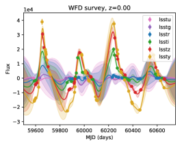
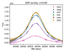
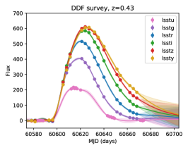
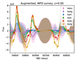
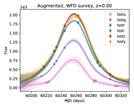
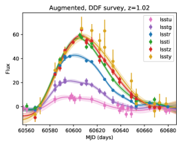
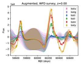
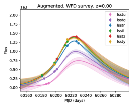
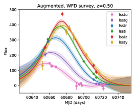
References
- Ambikasaran et al. (2015) Ambikasaran, S., Foreman-Mackey, D., Greengard, L., Hogg, D. W., & O’Neil, M. 2015, IEEE Transactions on Pattern Analysis and Machine Intelligence, 38, 252
- Astier et al. (2006) Astier, P., Guy, J., Regnault, N., et al. 2006, A&A, 447, 31
- Astropy Collaboration et al. (2013) Astropy Collaboration, Robitaille, T. P., Tollerud, E. J., et al. 2013, A&A, 558, A33
- Astropy Collaboration et al. (2018) Astropy Collaboration, Price-Whelan, A. M., Sipőcz, B. M., et al. 2018, AJ, 156, 123
- Bailey et al. (2007) Bailey, S., Aragon, C., Romano, R., et al. 2007, ApJ, 665, 1246
- Beers et al. (1990) Beers, T. C., Flynn, K., & Gebhardt, K. 1990, AJ, 100, 32
- Bernstein et al. (2012) Bernstein, J. P., Kessler, R., Kuhlmann, S., et al. 2012, ApJ, 753, 152
- Betoule et al. (2014) Betoule, M., Kessler, R., Guy, J., et al. 2014, A&A, 568, A22
- Charnock & Moss (2017) Charnock, T., & Moss, A. 2017, ApJ, 837, L28
- Delgado et al. (2014) Delgado, F., Saha, A., Chandrasekharan, S., et al. 2014, in Proc. SPIE, Vol. 9150, Modeling, Systems Engineering, and Project Management for Astronomy VI, 915015
- Fakhouri et al. (2015) Fakhouri, H. K., Boone, K., Aldering, G., et al. 2015, ApJ, 815, 58
- Guy et al. (2007) Guy, J., Astier, P., Baumont, S., et al. 2007, A&A, 466, 11
- Hlozek et al. (2012) Hlozek, R., Kunz, M., Bassett, B., et al. 2012, ApJ, 752, 79
- Hunter (2007) Hunter, J. D. 2007, Computing in Science & Engineering, 9, 90
- Ishida & de Souza (2013) Ishida, E. E. O., & de Souza, R. S. 2013, MNRAS, 430, 509
- Ishida et al. (2019) Ishida, E. E. O., Beck, R., González-Gaitán, S., et al. 2019, MNRAS, 483, 2
- Jones et al. (2017) Jones, D. O., Scolnic, D. M., Riess, A. G., et al. 2017, ApJ, 843, 6
- Jones et al. (2001) Jones, E., Oliphant, T., Peterson, P., et al. 2001, SciPy: Open source scientific tools for Python, v1.2.1, Online, [accessed 6/3/2019]. http://www.scipy.org/
- Kaiser et al. (2010) Kaiser, N., Burgett, W., Chambers, K., et al. 2010, in Proc. SPIE, Vol. 7733, Ground-based and Airborne Telescopes III, 77330E
- Karpenka et al. (2013) Karpenka, N. V., Feroz, F., & Hobson, M. P. 2013, MNRAS, 429, 1278
- Ke et al. (2017) Ke, G., Meng, Q., Finley, T., et al. 2017, in Advances in Neural Information Processing Systems 30, ed. I. Guyon, U. V. Luxburg, S. Bengio, H. Wallach, R. Fergus, S. Vishwanathan, & R. Garnett (Curran Associates, Inc.), 3146–3154
- Kelly et al. (2010) Kelly, P. L., Hicken, M., Burke, D. L., Mandel, K. S., & Kirshner, R. P. 2010, ApJ, 715, 743
- Kessler et al. (2009) Kessler, R., Bernstein, J. P., Cinabro, D., et al. 2009, PASP, 121, 1028
- Kessler et al. (2010) Kessler, R., Bassett, B., Belov, P., et al. 2010, PASP, 122, 1415
- Kessler et al. (2015) Kessler, R., Marriner, J., Childress, M., et al. 2015, AJ, 150, 172
- Kessler et al. (2019) Kessler, R., Narayan, G., Avelino, A., et al. 2019, arXiv e-prints, arXiv:1903.11756
- Kim et al. (2013) Kim, A. G., Thomas, R. C., Aldering, G., et al. 2013, ApJ, 766, 84
- Kluyver et al. (2016) Kluyver, T., Ragan-Kelley, B., Pérez, F., et al. 2016, in Positioning and Power in Academic Publishing: Players, Agents and Agendas, ed. F. Loizides & B. Schmidt, IOS Press, 87 – 90
- Knop et al. (2003) Knop, R. A., Aldering, G., Amanullah, R., et al. 2003, ApJ, 598, 102
- Kowalski et al. (2008) Kowalski, M., Rubin, D., Aldering, G., et al. 2008, ApJ, 686, 749
- Kunz et al. (2007) Kunz, M., Bassett, B. A., & Hlozek, R. A. 2007, Phys. Rev. D, 75, 103508
- Lochner et al. (2016) Lochner, M., McEwen, J. D., Peiris, H. V., Lahav, O., & Winter, M. K. 2016, ApJS, 225, 31
- LSST Science Collaboration et al. (2009) LSST Science Collaboration, Abell, P. A., Allison, J., et al. 2009, arXiv e-prints, arXiv:0912.0201
- Malz et al. (2018) Malz, A., Hložek, R., Allam, Jr, T., et al. 2018, arXiv e-prints, arXiv:1809.11145
- McKinney (2010) McKinney, W. 2010, in Proceedings of the 9th Python in Science Conference, ed. S. van der Walt & J. Millman, 51 – 56
- Oke & Sandage (1968) Oke, J. B., & Sandage, A. 1968, ApJ, 154, 21
- Okumura et al. (2014) Okumura, J. E., Ihara, Y., Doi, M., et al. 2014, PASJ, 66, 49
- Pasquet et al. (2019) Pasquet, J., Pasquet, J., Chaumont, M., & Fouchez, D. 2019, arXiv e-prints, arXiv:1901.01298
- Pedregosa et al. (2011) Pedregosa, F., Varoquaux, G., Gramfort, A., et al. 2011, Journal of Machine Learning Research, 12, 2825
- Perlmutter et al. (1999) Perlmutter, S., Aldering, G., Goldhaber, G., et al. 1999, ApJ, 517, 565
- PLAsTiCC Team and PLAsTiCC Modelers (2019) PLAsTiCC Team and PLAsTiCC Modelers. 2019, Unblinded Data for PLAsTiCC Classification Challenge, Zenodo, doi:10.5281/zenodo.2539456. https://doi.org/10.5281/zenodo.2539456
- Poznanski et al. (2007) Poznanski, D., Maoz, D., & Gal-Yam, A. 2007, AJ, 134, 1285
- Rasmussen & Williams (2006) Rasmussen, C. E., & Williams, C. K. I. 2006, Gaussian Processes for Machine Learning (The MIT Press)
- Revsbech et al. (2018) Revsbech, E. A., Trotta, R., & van Dyk, D. A. 2018, MNRAS, 473, 3969
- Richards et al. (2012) Richards, J. W., Homrighausen, D., Freeman, P. E., Schafer, C. M., & Poznanski, D. 2012, MNRAS, 419, 1121
- Riess et al. (1998) Riess, A. G., Filippenko, A. V., Challis, P., et al. 1998, AJ, 116, 1009
- Riess et al. (2004) Riess, A. G., Strolger, L.-G., Tonry, J., et al. 2004, ApJ, 607, 665
- Rigault et al. (2013) Rigault, M., Copin, Y., Aldering, G., et al. 2013, A&A, 560, A66
- Rodney et al. (2014) Rodney, S. A., Riess, A. G., Strolger, L.-G., et al. 2014, AJ, 148, 13
- Rubin et al. (2015) Rubin, D., Aldering, G., Barbary, K., et al. 2015, ApJ, 813, 137
- Sako et al. (2011) Sako, M., Bassett, B., Connolly, B., et al. 2011, ApJ, 738, 162
- Saunders et al. (2018) Saunders, C., Aldering, G., Antilogus, P., et al. 2018, ApJ, 869, 167
- Scolnic et al. (2018) Scolnic, D. M., Jones, D. O., Rest, A., et al. 2018, ApJ, 859, 101
- Stein (1999) Stein, M. L. 1999, Interpolation of spatial data, Springer Series in Statistics (New York: Springer-Verlag), xviii+247, some theory for Kriging, doi:10.1007/978-1-4612-1494-6. http://dx.doi.org/10.1007/978-1-4612-1494-6
- Strolger et al. (2015) Strolger, L.-G., Dahlen, T., Rodney, S. A., et al. 2015, ApJ, 813, 93
- Suzuki et al. (2012) Suzuki, N., Rubin, D., Lidman, C., et al. 2012, ApJ, 746, 85
- The Dark Energy Survey Collaboration (2005) The Dark Energy Survey Collaboration. 2005, arXiv e-prints, astro
- The LSST Dark Energy Science Collaboration et al. (2018) The LSST Dark Energy Science Collaboration, Mandelbaum, R., Eifler, T., et al. 2018, arXiv e-prints, arXiv:1809.01669
- van der Walt et al. (2011) van der Walt, S., Colbert, S. C., & Varoquaux, G. 2011, Computing in Science and Engineering, 13, 22
- VanderPlas (2018) VanderPlas, J. T. 2018, The Astrophysical Journal Supplement Series, 236, 16