Fragmentation of Filamentary Cloud Permeated by Perpendicular Magnetic Field II.
Dependence on the Initial Density Profile

Abstract

We examine the linear stability of a filamentary cloud permeated by a perpendicular magnetic field. The initial magnetic field is assumed to be uniform and perpendicular to the cloud axis. The model cloud is assumed to have a Plummer-like density profile and to be supported against the self-gravity by turbulence. The effects of turbulence are taken into account by enhancing the effective pressure of a low density gas. We derive the effective pressure as a function of the density from the condition of the hydrostatic balance. It is shown that the model cloud is more unstable against radial collapse, when the radial density slope is shallower. When the magnetic field is mildly strong, the radial collapse is suppressed. If the displacement vanishes in the region very far from the cloud axis, the model cloud is stabilized completely by a mildly strong magnetic field. If rearrangement of the magnetic flux tubes is permitted, the model cloud is unstable even when the magnetic field is extremely strong. The stability depends on the outer boundary condition as in case of the isothermal cloud. The growth rate of the rearrangement mode is smaller when the radial density slope is shallower.

=3

1 INTRODUCTION

Filamentary structures are ubiquitously found in the star-forming regions (see, e.g., André et al., 2014, and the references therein). They are considered as an intermediate state from clouds to stars and the fragmentation is likely to be a process forming cores. This idea is supported by observations showing that prestellar cores and newly formed stars are associated with the dense parts of filamentary clouds. Although filamentary clouds are unstable against fragmentation in general (see, e.g., Stodólkiewicz, 1963; Larson, 2003), a magnetic field may suppress the fragmentation if it is strong and perpendicular to the cloud axis. The effect of the magnetic field on fragmentation is a key issue for understanding the core formation.

We have examined the stability of a filamentary cloud permeated by a perpendicular magnetic field against fragmentation using a simplified model (Hanawa, Kudoh & Tomisaka, 2017, paper I in the following). The initial magnetic field was assumed to be uniform and the gas was assumed to be isothermal in paper I for simplicity. These assumptions are made from technical reasons that it is difficult to make an equilibrium model for molecular cloud permeated by a perpendicular cloud (see, e.g., Tomisaka, 2014; Hanawa & Tomisaka, 2015). When the magnetic field is parallel to the cloud axis or helical around the axis, we can make various equilibrium models by assuming symmetry around the cloud axis (see, e.g., Toci & Galli, 2015b). Such model clouds have been studied extensively for many years (Stodólkiewicz, 1963; Nakamura, Hanawa & Nakano, 1993; Hanawa et al., 1993; Fiege & Pudritz, 2000). However, the magnetic fields are perpendicular to denser clouds (see, e.g., Sugitani et al., 2011; André et al., 2014; Kusune et al., 2016; Soler et al., 2016), although less dense clouds are associated with parallel magnetic fields.

Magnetic field direction is important to fragmentation of a filamentary cloud. A magnetic force is perpendicular to the magnetic fields and hence gas flow along the axis can not be suppressed by magnetic fields parallel to the axis. The wavelength of fragmentation is shorter when the parallel magnetic field is stronger. This apparent destabilizing effect is ascribed to the fact that the magnetic field is assumed to be concentrated around the axis to support the cloud against the radial collapse. Given the central density and temperature, the filament diameter is larger for a stronger magnetic field. The wavelength of the fragmentation, which is roughly twice of the Jeans length, is shorter for a stronger magnetic field, when measure in unit of the diameter. Moreover, the mass to flux ratio is infinitely large, and hence supercritical if the cloud is elongated along the magnetic field. When the magnetic field is perpendicular to the cloud axis, the magnetic force works against fragmentation (paper I). Even mildly strong magnetic fields stabilize a filamentary cloud against fragmentation, if they are perpendicular to the cloud and their ends are fixed in the region very far from the cloud. When the magnetic field is helical around the axis, the magnetic force works against fragmentation but induces non-axisymmetric instability (see, e.g., Hanawa et al., 1993; Fiege & Pudritz, 2000).

Interestingly perpendicular magnetic fields suppress instability less effectively if the field lines are free, i.e., allowed to move. When the magnetic fields are free in the region very far from the cloud, they are rearranged to fragment the cloud by reducing the gravitational energy of the cloud. This means that the stability depends on the outer boundary condition. When the magnetic fields are parallel to the cloud axis, boundary condition has little effects on the instability unless they are placed close to the cloud axis. This is reasonable since the instability is due to the self-gravity of the cloud and depends only on the dense central gas.

In paper I the model cloud is assumed to be isothermal and supported by gas pressure alone against gravity in equilibrium. Accordingly, the density is assumed to decrease in proportion to $r^{-4}$ in the region very far from the cloud center, where $r$ denotes the distance from the cloud axis. However, observed clouds show much shallower radial density profiles, which is often approximated by a Plummer-like one,

$$\rho(r) = \rho_{c}\left[1+\left(\frac{r}{R_{\rm flat}}\right)^{2}\right]^{-p/2},$$ (1)

where $\rho_{c}$ and $R_{\rm flat}$ denote the central density and ‘radius’, respectively (Arzoumanian et al., 2011; Juvela et al., 2012; Palmeirim et al., 2013; Ohashi et al., 2018). The index, $p$, denotes the slope of the density profile, $-d\ln\rho/d\ln r$, in the region far from the cloud axis. The index is estimated to be $p\approx 2$ from the model fit to the column density distribution derived from the sub-millimeter continuum emission.

Considering the above mentioned arguments, we examine the stability of the Plummer-like cloud against fragmentation taking account of perpendicular magnetic fields. We assume that the Plummer-like profile is supported against gravity by ‘effective gas pressure’, which mimics effects of turbulence. If the effective temperature decreases with increase in the density, the Plummer-like profile with $p<4$ is realized as will be shown later. We examine the effects of the density profile on fragmentation of a filamentary cloud using the method developed in paper I. When $p<4$, the model cloud is unstable also against radial collapse, although the isothermal model is neutrally stable against it (see, e.g., the review by Larson, 2003). It will be shown that the radial collapse is stabilized by mildly strong magnetic fields. The growth rate of the instability depends on the index, $p$, but only quantitatively except for the radial collapse.

This paper is organized as follows. We describe our assumptions and methods for computation in §2. The results are shown in §3, where also the stability of unmagnetized cloud is analyzed. We discuss the implications of our models in §4 and summarize our main findings in §5. Appendices A and B are devoted to improvement for computing long wavelength modes and computing the case of no magnetic fields, respectively.

2 METHODS

2.1 Basic Equations

As in paper I, we employ the ideal magnetohydrodymamic (MHD) equations for our stability analysis. They are expressed as

$$\frac{\partial\rho}{\partial t}+\mbox{\boldmath$\nabla$}\cdot\left(\rho\mbox{\boldmath$v$}\right)=0,$$ (2)

$$\rho\frac{d\mbox{\boldmath$v$}}{dt}=-\mbox{\boldmath$\nabla$}P+\mbox{\boldmath$j$}\times\mbox{\boldmath$B$}-\rho\mbox{\boldmath$\nabla$}\Phi,$$ (3)

$$\mbox{\boldmath$j$}=\frac{\mbox{\boldmath$\nabla$}\times\mbox{\boldmath$B$}}{4\pi},$$ (4)

where $\rho$, $\Phi$, $v$, $B$, and $j$ denote the density, gravitational potential, velocity, magnetic field, and electric current density, respectively. Here the symbol, $P$, denotes the pressure, which is designed to include effects of turbulence implicitly.

We ignore ambipolar diffusion for simplicity. The ambipolar diffusion weakens the magnetic force (see, e.g. Hosseinirad et al., 2018). However, the typical timescale is a factor ten longer than the dynamical timescale (see, e.g., Nakano & Umebayashi, 1988) and the effects are not large. Thus we do not take account of the ambipolar diffusion in order to avoid further complication. Note that the ambipolar diffusion does not work in our initial model since the magnetic field is uniform. The ambipolar diffusion works works only on a perturbation. Thus, it reduces the growth rate of instability but cannot suppress the stability. See e.g., Hosseinirad et al. (2018) for the effects of ambipolar diffusion on the fragmentation. They analyzed the stability of a filamentary cloud permeated by longitudinal magnetic field.

The equation of state is specified in the subsequent section so that the equilibrium density distribution is well approximated by the Plummer function,

$$\rho_{0} = \rho_{c}\left(1+\frac{r^{2}}{2pH^{2}}\right)^{-p/2},$$ (5)

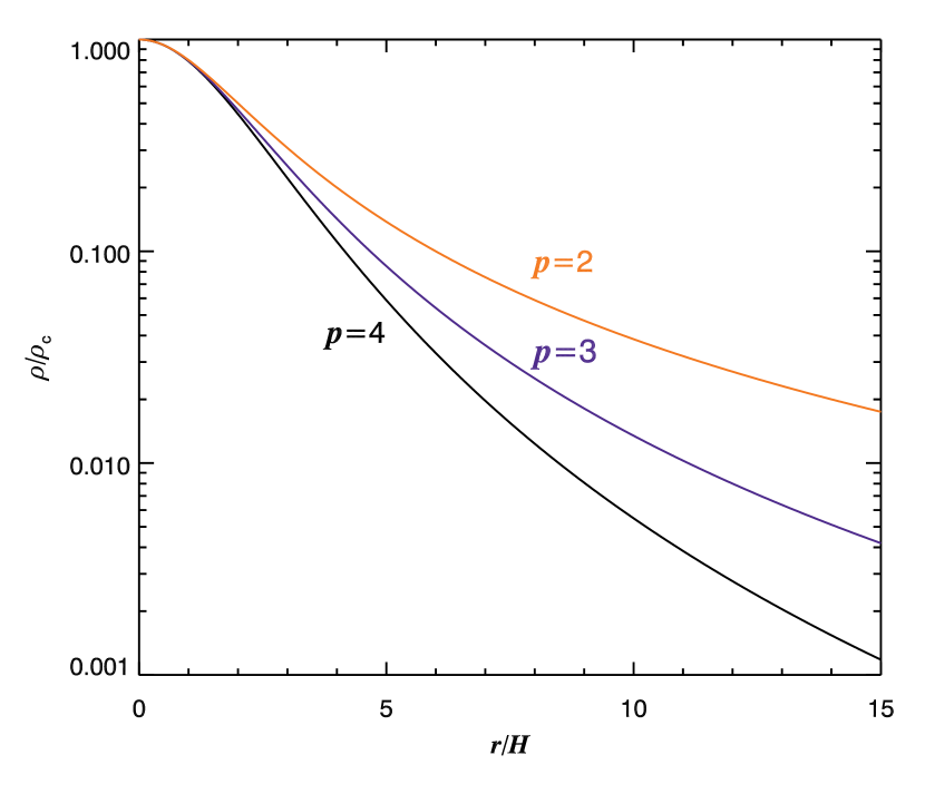
where $\rho_{c}$ and $r$ denote the central density of the filamentary cloud and the distance from the cloud axis, respectively. The symbols, $p$ and $H$, denote the index and length scale, respectively. The length scale given in Equation (1) is expressed as $R_{\rm flat}=\sqrt{2p}H$. The radial density profile is shown in Figure 1.

Figure 1: Equilibrium density profiles for the index of $p$ = 2, 3, and 4.

The self-gravity of the gas is taken into account through Poisson’s equation,

$$\Delta\Phi=4\pi G\rho,$$ (6)

where $G$ denotes the gravitational constant.

In the following, we use the unit system where $\rho_{c}=1$, $H=1$ and $4\pi G\rho_{c}=1$, in our numerical computations.

2.2 Equilibrium Model

When the density profile is expressed by Equation (5), the filamentary cloud has the mass per unit length,

$$\lambda_{r} = 2\pi\int_{0}^{r}\rho_{0}\left(r^{\prime}\right)r^{\prime}dr^{\prime}$$ (7)

$$= \begin{cases}\displaystyle 4\pi\rho_{c}H^{2}\ln\left(1+\frac{r^{2}}{4H^{2}}\right)&(p=2)\\ \displaystyle\frac{4\pi p\rho_{c}H^{2}}{p-2}\left[1-\left(1+\frac{r^{2}}{2pH^{2}}\right)^{1-p/2}\right]&\mbox{(otherwise)}\end{cases},$$ (8)

inside the radius, $r$. Thus the gravity is evaluated to be

$$g_{r} = -\frac{d\Phi}{dr}=-\frac{2G\lambda_{r}}{r}$$ (9)

$$= \begin{cases}-\displaystyle\frac{8\pi G\rho_{c}H^{2}}{r}\ln\left(1+\frac{r^{2}}{4H^{2}}\right)&(p=2)\\ -\displaystyle\frac{8\pi Gp\rho_{c}H^{2}}{\left(p-2\right)r}\left[1-\left(1+\frac{r^{2}}{2pH^{2}}\right)^{1-p/2}\right]&\mbox{(otherwise)}\end{cases}.$$ (10)

We assume that our model cloud is supported by pressure alone in equilibrium against the gravity for simplicity. This assumption means that the magnetic field is assumed to be uniform. This may a crude assumption and the magnetic field is likely to be concentrated in a dense cloud. However, it is very difficult to take account of non-uniform magnetic field (see, e.g., Tomisaka, 2014). The observed radial volume density profile is also derived from the projected surface density under the assumption that the cloud is symmetric around the axis. Thus, it is worth to analyze this very simplified model.

Since the pressure gradient is given by

$$\frac{dP_{0}}{dr} = \rho_{0}g_{r},$$ (11)

the pressure and the density should satisfy the relation,

$$\frac{dP_{0}}{d\rho_{0}}=\left(\frac{dP_{0}}{dr}\right)\left(\frac{d\rho_{0}}{dr}\right)^{-1}.$$ (12)

When $p=2$, the right-hand side of equation (12) is evaluated to be

$$\frac{dP_{0}}{d\rho_{0}} = \frac{4\pi GH^{2}\rho_{c}^{2}}{\rho_{c}-\rho_{0}}\ln\left(\frac{\rho_{c}}{\rho_{0}}\right),$$ (13)

where equations (5) and (10) are substituted into equation (11). Otherwise, it is evaluated to be

$$\frac{dP_{0}}{d\rho_{0}} = \frac{8\pi G\rho_{c}H^{2}}{p-2}\left(\frac{2pH^{2}}{r^{2}}\right)\left(1+\frac{r^{2}}{2pH^{2}}\right)\left[1-\left(1+\frac{r^{2}}{2pH^{2}}\right)^{1-p/2}\right]$$ (14)

$$= \frac{8\pi G\rho_{c}H^{2}}{p-2}\left[1-\left(\frac{\rho}{\rho_{c}}\right)^{2/p}\right]^{-1}\left[1-\left(\frac{\rho}{\rho_{c}}\right)^{1-2/p}\right].$$

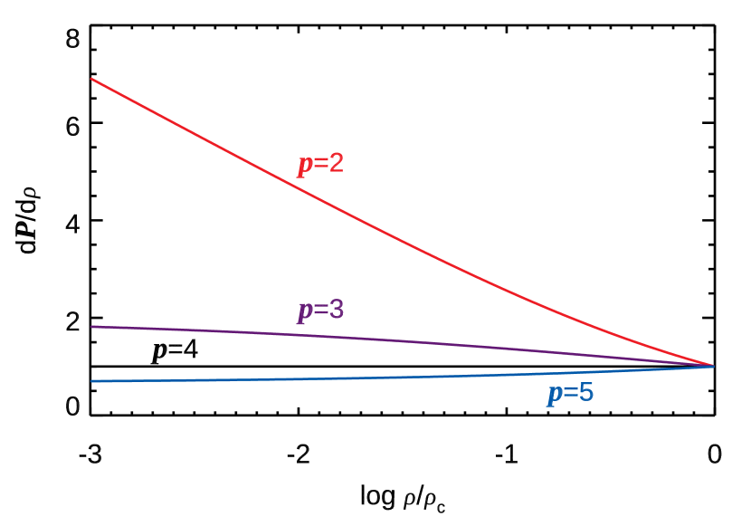
In the following, we assume that Equations (13) and (14) hold not only in the equilibrium but also for a perturbation. Thus we use the symbol $dP/d\rho$ instead of $dP_{0}/d\rho_{0}$. Figure 2 shows the value as a function of $\log\left(\rho/\rho_{c}\right)$ in unit of $4\pi G\rho_{c}H^{2}$. The sound speed ($\sqrt{dP/d\rho}$) decreases with increasing density for $p<4$, while it increases for $p>4$. In this paper we restrict ourselves to the case of $p\leq 4$, since the velocity turbulence is lower in a region of higher density in the interstellar medium. Thus it is similar to the logatrope proposed by McLaughlin & Pudritz (1996). They introduced an effective equation of state,

$$P = P_{c}\left[1+\kappa\ln\left(\frac{\rho}{\rho_{c}}\right)\right],$$ (15)

to mimic interstellar turbulence, where $P_{c}$, $\rho_{c}$, and $\kappa$ denote model parameters. However, the dependence of the sound speed on the density is weaker than that for logatrope, since Equation (15) means

$$\frac{dP}{d\rho} = \kappa\frac{P_{c}}{\rho}.$$ (16)

We examine equation (14) again in §4.

Figure 2: The sound speed squared, $(dP/d\rho)$, is shown as a function of $\log(\rho/\rho)$ for $p$ = 2, 3, 4, and 5 in units of $4\pi G\rho_{c}H^{2}$.

We assume that the magnetic field is uniform and runs in the $x$-direction in the equilibrium. To specify the initial magnetic field strength in the analysis, we use the plasma beta at the cloud center,

$$\beta = \frac{8\pi\rho_{c}}{B_{0}^{2}}\left(\frac{dp}{d\rho}\right)_{\rho=\rho_{c}}=\frac{32\pi G\rho_{c}^{2}H^{2}}{B_{0}^{2}},$$ (17)

as in paper I. The plasma beta is related to the mass to flux ratio,

$$f = \frac{\displaystyle\int\rho_{0}(x^{\prime},y,z)dx^{\prime}}{B_{0}}\;=\;\frac{\sqrt{2\pi p}\Gamma\displaystyle\left(\frac{p-1}{2}\right)}{\Gamma\displaystyle\left(\frac{p}{2}\right)}\left(1+\frac{y^{2}}{2pH^{2}}\right)^{(-p+1)/2}\frac{\rho_{c}H}{B_{0}},$$ (18)

where $\Gamma$ denotes the gamma function. When the mass to flux ratio is critical, i.e., $f_{c}=\left(2\pi\sqrt{G}\right)^{-1}$, the plasma beta is $\beta=2/\pi^{2}$, $1/3$, and $4/\pi^{2}$ for $p$ = 2, 3, and 4, respectively.

2.3 Perturbation Equation

Following paper I, we consider a small perturbation around the equilibrium in order to search for an unstable mode. The perturbation is described by the displacement defined by

$$\xi = e^{\sigma t}\left[\xi_{x}(x,y)\cos kz\mbox{\boldmath${e}$}_{x}+\xi_{y}(x,y)\cos kz\mbox{\boldmath$e$}_{y}+\xi_{z}(x,y)\sin kz\mbox{\boldmath$e$}_{z}\right],$$ (19)

where the perturbation is assumed to be sinusoidal in the $z$-direction with the wavenumber $k$ and to grow exponentially with time at the rate, $\sigma$. The change in the density is described as

$$\rho(x,y,z,t) = \rho_{0}(x,y)+e^{\sigma t}\delta\varrho(x,y)\cos kz.$$ (20)

Substituting $\mbox{\boldmath$v$}=d\mbox{\boldmath$\xi$}/dt$ and Equation (19) into Equation (2) we obtain

$$\delta\varrho = -\frac{\partial}{\partial x}\left(\rho_{0}\xi_{x}\right)-\frac{\partial}{\partial y}\left(\rho_{0}\xi_{y}\right)-k\rho_{0}\xi_{z}.$$ (21)

Similarly, we obtain the perturbation in the magnetic field from the induction equation,

$$\delta\mbox{\boldmath$B$}=\mbox{\boldmath$\nabla$}\times\left(\mbox{\boldmath$\xi$}\times\mbox{\boldmath$B$}_{0}\right).$$ (22)

The induction equation is further expressed as

$$\delta\mbox{\boldmath$B$}(x,y,z) = b_{x}(x,y)\cos kz\mbox{\boldmath$e$}_{x}+b_{y}(x,y)\cos kz\mbox{\boldmath$e$}_{y}+b_{z}(x,y)\sin kz\mbox{\boldmath$e$}_{z},$$ (23)

$$b_{x} = -B_{0}\left(\frac{\partial}{\partial y}\xi_{y}+k\xi_{z}\right),$$ (24)

$$b_{y} = B_{0}\frac{\partial\xi_{y}}{\partial x},$$ (25)

$$b_{z} = B_{0}\frac{\partial\xi_{z}}{\partial x}.$$ (26)

We evaluate the change in the current density to be

$$\delta\mbox{\boldmath$J$}=\frac{1}{4\pi}\mbox{\boldmath$\nabla$}\times\delta\mbox{\boldmath$B$},$$ (27)

using Equation (4). Each component of the current density is expressed as

$$\delta\mbox{\boldmath$J$}(x,y,z) = j_{x}(x,y)\sin kz\mbox{\boldmath$e$}_{x}+j_{y}(x,y)\sin kz\mbox{\boldmath$e$}_{y}+j_{z}(x,y)\cos kz\mbox{\boldmath$e$}_{z},$$ (28)

$$j_{x} = \frac{1}{4\pi}\left(\frac{\partial b_{z}}{\partial y}+kb_{y}\right),$$ (29)

$$j_{y} = -\frac{1}{4\pi}\left(kb_{x}+\frac{\partial b_{z}}{\partial x}\right),$$ (30)

$$j_{z} = \frac{1}{4\pi}\left(\frac{\partial b_{y}}{\partial x}-\frac{\partial b_{x}}{\partial y}\right).$$ (31)

Then the changes in the density and current density are expressed as an explicit function of $\xi$.

The change in the gravitational potential is given as the solution of the Poisson equation

$$\mbox{\boldmath$\nabla$}^{2}\delta\psi=4\pi G\delta\rho.$$ (32)

Thus, it can be regarded as an implicit function of $\xi$.

We derive the equation of motion for the perturbation by taking account of the force balance,

$$\left(\frac{dP}{d\rho}\right)\mbox{\boldmath$\nabla$}\rho_{0}+\rho_{0}\mbox{\boldmath$\nabla$}\psi_{0}=0,$$ (33)

with no electric current density, $\mbox{\boldmath$j$}_{0}=0$, in equilibrium. Then the equation of motion is expressed as

$$\sigma^{2}\rho_{0}\mbox{\boldmath$\xi$}=-\rho_{0}\mbox{\boldmath$\nabla$}\left(\frac{dP}{d\rho}\frac{\delta\rho}{\rho_{0}}\right)-\rho_{0}\nabla\delta\psi+\delta\mbox{\boldmath$J$}\times\mbox{\boldmath$B$}_{0},$$ (34)

where the last term represents the magnetic force. The term, $\mbox{\boldmath$J$}_{0}\times\delta\bm{\boldmath$B$}$, does not appear in Equation (34) since $\mbox{\boldmath$J$}_{0}=0$ in our equilibrium model. The linear growth rate, $\sigma$, is obtained as the eigenvalue of the differential equation (34), since the right-hand side is proportional to $\xi$.

The derived perturbation equations are the same as those derived in paper I except for the sound speed ($\sqrt{dP/d\rho}$), which is a function of the density in our analysis but constant in paper I.

Table 1: Variables Describing Perturbations

variable	evaluation	symmetry	symmetry
	point	$x$	$y$
$\xi_{x}$	$(i-1/2,j)$	A	S
$\xi_{y}$	$(i,j-1/2)$	S	A
$\xi_{z}$	$(i,j)$	S	S
$\delta\varrho$	$(i,j)$	S	S
$\delta\psi$	$(i,j)$	S	S
$b_{x}$	$(i,j)$	S	S
$b_{y}$	$(i-1/2,j-1/2)$	A	A
$b_{z}$	$(i-1/2,j)$	A	S
$j_{y}$	$(i,j)$	S	S
$j_{z}$	$(i,j-1/2)$	S	A

Our equilibrium model is symmetric with respect to the $x$- and $y$-axes. Thus, all eigenmodes should be either symmetric or anti-symmetric with respect to these axes. We restrict ourselves to the eigenmodes symmetric to both $x$- and $y$-axes, since the unstable mode has the same symmetry in the case of no magnetic field (Nakamura, Hanawa & Nakano, 1993). The choice of this symmetry is justified since we are interested only in the unstable mode. Using this symmetry, we can reduce the region of computation to the first quadrant, $x\geq 0$ and $y\geq 0$. The variables describing the perturbation and their symmetries are summarized in Table 1.

We consider two types of the boundary conditions. The first one assumes that the displacement should vanish in the region very far from the filament center. We call this the fixed boundary since the magnetic field lines are fixed on the boundary. The second one allows the magnetic field lines to move while remaining straight and normal to the boundary. This restriction is expressed as

$$\left(\mbox{\boldmath$B$}_{0}\cdot\mbox{\boldmath$\nabla$}\right)\mbox{\boldmath$\xi$}=0.$$ (35)

Thus, we assume $\partial\mbox{\boldmath$\xi$}/\partial x$ on the boundary in the $x$-direction and $\mbox{\boldmath$\xi$}=0$ in the $y$-direction. We refer to this as the free boundary condition. In both types of boundary conditions, we use the symmetries given in Table 1 to set the boundary conditions for $x=0$ and $y=0$.

2.4 Numerical Methods

We solve the eigenvalue problem numerically by a finite difference approach. The differential equations are evaluated on the rectangular grid in the $xy$ plane. We evaluate $\xi_{z}$, $\delta\varrho$, $\delta\psi$, $b_{x}$, and $j_{y}$ at the points

$$\left(x_{i},y_{j}\right) = \left(i\Delta x,j\Delta y\right),$$ (36)

where $i$ and $j$ specify the grid points, while $\Delta x$ and $\Delta y$ denote the grid spacing in the $x$- and $y$-directions, respectively (see Table 1). These variables are symmetric with respect to both the $x$- and $y$-axes. Using this symmetry, we consider the range $0\leq i\leq n_{x}$ and $0\leq j\leq n_{y}$, where $n_{x}$ and $n_{y}$ specify the number of grid points in each direction. When $i>n_{x}$ or $j>n_{y}$, the displacement $\xi_{z,i,j}$ is assumed to vanish for the fixed boundary and to have the same values at neighboring points in the computation domain for the free boundary condition. We use the indexes, $i$ and $j$, to specify the position where the variables are evaluated, such as $\xi_{z,i,j}=\xi_{z}(x_{i},y_{j})$.

The variables are evaluated at either of

$$\left(x_{i-1/2},y_{j}\right) = \left[\left(i-\frac{1}{2}\right)\Delta x,j\Delta y\right],$$ (37)

$$\left(x_{i},y_{j-1/2}\right) = \left[i\Delta x,\left(j-\frac{1}{2}\right)\Delta y\right],$$ (38)

$$\left(x_{i-1/2},y_{j-1/2}\right) = \left[\left(i-\frac{1}{2}\right)\Delta x,\left(j-\frac{1}{2}\right)\Delta y\right].$$ (39)

depending on the symmetry as summarized in Table 1. Here the symbols, $i$ and $j$, are integers to specify the grid points while $\Delta x$ and $\Delta y$ denote the grid spacings in the $x$- and $y$-directions, respectively. All these variables are evaluated in the region $0\leq x\leq n_{x}\Delta x$ and $0\leq y\leq n_{y}\Delta y$. In other words, we use staggered this kind of grids to achieve second-order accuracy in space.

Using the variables defined on the grids, we rewrite the perturbation equations. Equation (21) is rewritten as

$$\delta\varrho_{i,j} = -\frac{\rho_{0,i+1/2,j}\xi_{x,i+1/2,j}-\rho_{0,i-1/2,j}\xi_{x,i-1/2,j}}{\Delta x}-\frac{\rho_{0,i,j+1/2}\xi_{y,i,j+1/2}-\rho_{0,i,j-1/2}\xi_{y,i,j-1/2}}{\Delta y}-k\rho_{0,i,j}\xi_{z,i,j}.$$ (40)

Equation (32), the Poisson equation, is expressed as

$$\frac{\delta\psi_{i+1,j}+\delta\psi_{i-1,j}}{\Delta x^{2}}+\frac{\delta\psi_{i,j+1}+\delta\psi_{i,j-1}}{\Delta y^{2}}-\left(\frac{2}{\Delta x^{2}}+\frac{2}{\Delta y^{2}}+k^{2}\right)\delta\psi_{j,k}=4\pi G\delta\varrho_{i,j}.$$ (41)

The solution of Equation (41) is expressed as

$$\delta\psi_{i,j} = \sum_{i^{\prime}}\sum_{j^{\prime}}G_{i,j,i^{\prime},j^{\prime}}\delta\varrho_{i^{\prime},j^{\prime}},$$ (42)

where $G_{i,j,i^{\prime},j^{\prime}}$ denotes the Green’s function and the value is obtained by solving Equation (41) numerically. The boundary condition for the Poisson equation is improved for increasing the accuracy of the growth at a small $k$. See Appendix A for more details.

The change in the magnetic field is evaluated as

$$b_{x,i,j} = -B_{0}\left(\frac{\xi_{y,i,j+1/2}-\xi_{y,i,j-1/2}}{\Delta y}+k\xi_{z,i,j}\right),$$ (43)

$$b_{y,i-1/2,j-1/2} = B_{0}\left(\frac{\xi_{y,i,j-1/2}-\xi_{y,i-1,j-1/2}}{\Delta x}\right),$$ (44)

$$b_{z,i-1/2,j} = B_{0}\left(\frac{\xi_{z,i,j}-\xi_{z,i-1,j}}{\Delta x}\right),$$ (45)

from Equations (24) through (26). The current density is evaluated as

$$j_{y,i,j} = -\frac{1}{4\pi}\left(kb_{x,i,j}+\frac{b_{z,i+1/2,j}-b_{z,i-1/2,j}}{\Delta x}\right),$$ (46)

$$j_{z,i,j-1/2} = \frac{1}{4\pi}\left(\frac{b_{y,i+1/2,j-1/2}-b_{y,i-1/2,j-1/2}}{\Delta x}-\frac{b_{x,i,j}-b_{x,i,j-1}}{\Delta y}\right).$$ (47)

The $x$-component of the current density, $j_{x}$, is not evaluated, since it does not appear in the equation of motion. The fixed boundary conditions are expressed as

$$\xi_{x,n_{x}+1/2,j} = 0,$$ (48)

$$\xi_{y,n_{x}+1,j-1/2} = 0,$$ (49)

$$\xi_{z,n_{x}+1,j} = 0,$$ (50)

$$\xi_{x,i-1/2,n_{y}+1} = 0,$$ (51)

$$\xi_{y,i,n_{y}+1/2} = 0,$$ (52)

$$\xi_{z,i,n_{y}+1} = 0.$$ (53)

When the free boundary is applied, the conditions are replaced with

$$\xi_{x,n_{x}+1/2,j} = \xi_{x,n_{x}-1/2,j},$$ (54)

$$\xi_{y,n_{x}+1,j-1/2} = \xi_{y,n_{x},j-1/2},$$ (55)

$$\xi_{z,n_{x}+1,j} = \xi_{z,n_{x},j},$$ (56)

$$\xi_{x,i-1/2,n_{y}+1} = \xi_{x,i-1/2,n_{y}},$$ (57)

$$\xi_{y,i,n_{y}+1/2} = \xi_{y,i,n_{y}-1/2},$$ (58)

$$\xi_{z,i,n_{y}+1} = \xi_{z,i,n_{y}}.$$ (59)

The equation of motion (34) is expressed as

$$\sigma^{2}\rho_{0,i-1/2,j}\xi_{x,i-1/2,j} = -\frac{\rho_{0,i-1/2,j}}{\Delta x}\left[\left(\frac{dP}{d\rho}\right)_{i,j}\frac{\delta\varrho_{i,j}}{\rho_{0,i,j}}-\left(\frac{dP}{d\rho}\right)_{i-1,j}\frac{\delta\varrho_{i-1,j}}{\rho_{0,i-1,j}}\right]-\frac{\rho_{0,i-1/2,j}}{\Delta x}\left(\delta\psi_{i,j}-\delta\psi_{i-1,j}\right).$$ (60)

$$\sigma^{2}\rho_{0,i,j-1/2}\xi_{y,i,j-1/2} = -\frac{\rho_{0,i,j-1/2}}{\Delta y}\left[\left(\frac{dP}{d\rho}\right)_{i,j}\frac{\delta\varrho_{i,j}}{\rho_{0,i,j}}-\left(\frac{dP}{d\rho}\right)_{i,j-1}\frac{\delta\varrho_{i,j-1}}{\rho_{0,i,j-1}}\right]-\frac{\rho_{0,i,j-1/2}}{\Delta y}\left(\delta\psi_{i,j}-\delta\psi_{i,j-1}\right)$$ (61)

$$+B_{0}j_{z,i,j-1/2}.$$

$$\sigma^{2}\rho_{0,i,j}\xi_{z,i,j} = -k\left(\frac{dP}{d\rho}\right)_{i,j}\delta\varrho_{i,j}-k\rho_{0,i,j}\delta\psi_{i,j}-B_{0}j_{y,i,j}.$$ (62)

Equations (60) through (62) are summarized in the form,

$$\sigma^{2}\mbox{\boldmath$B$}\mbox{\boldmath$\zeta$}=\left(\mbox{\boldmath$A$}+B_{0}^{2}\mbox{\boldmath$C$}\right)\mbox{\boldmath$\zeta$},$$ (63)

by using Equations (40), and (42) through (47). Here, $\zeta$ denotes an array of components, $\xi_{x,i-1/2,j}$, $\xi_{y,i,j-1/2}$, and $\xi_{z,i,j}$ for all the combinations of $i$ and $j$. The matrix elements of $A$, $B$, and $C$ are evaluated numerically as a function of $k$. See Appendix B of Paper I for further details. Then the growth rate is given as the solution of

$$\det\left(\sigma^{2}\mbox{\boldmath$B$}-\mbox{\boldmath$A$}-B_{0}^{2}\mbox{\boldmath$C$}\right)=0.$$ (64)

We rewrite Equation (64) into

$$\det\left[\sigma^{2}-\mbox{\boldmath$B$}^{-1/2}\left(\mbox{\boldmath$A$}-B_{0}^{2}\mbox{\boldmath$C$}\right)\mbox{\boldmath$B$}^{-1/2}\right]=0,$$ (65)

where matrix, $\mbox{\boldmath$B$}^{-1/2}$, is obtained easily since only the diagonal elements have non-zero values in matrix, $B$. Equation (65) is an eigenvalue problem while equation (64) is a generalized eigenvalue problem. Various library programs are available for solving the former. We use subroutine DGEEVX of LAPACK (see, Anderson et al., 1999, for the software) to solve Equation (65). The subroutine returns all the eigenvalues $\sigma^{2}$.

The matrixes $A$, $B$, and $C$ have dimension $\left(3n_{x}n_{y}+2n_{x}+2n_{y}+1\right)$. Thus, we obtain $3n_{x}n_{y}+2n_{x}+2n_{y}+1$ eigenmodes. However, we select only one unstable mode ($\sigma^{2}>10^{-5}$) for a given $k$ and $B_{0}$. The remaining eigenmodes denote oscillation of the filamentary cloud. In the following, we restrict ourselves to the unstable mode.

When $B_{0}=0$, our equilibrium model is symmetric around the axis and we can simplify the stability analysis using the cylindrical coordinates. The numerical methods are summarized in Appendix B.

When $k=0$, we need not solve Equation (62), since the $z$-component of the displacement, $\xi_{z}$, vanishes. Accordingly, we can omit the corresponding part of the matrix given Equation (65). The dimension of the matrix to be solved reduces to $2n_{x}n_{y}+n_{x}+n_{y}$. The boundary condition for the Poisson equation is given at the end of Appendix A.

3 RESULTS

3.1 Case of $B_{0}=0$

Before examining the effects of magnetic field, we analyze the stability of our Plummer-like model for the case of $B_{0}=0$. When the magnetic field vanishes, our equilibrium model is symmetric around the $z$-axis. Hence the stability analysis is reduced to 1D problem. We obtained the growth rate, $\sigma$, as a function of the wavenumber, $k$, for $p=2$, 3, and 4 according to the method given in Appendix B. The growth rate is obtained by solving the discretized perturbation equation with the spatial resolution, $\Delta r=0.1H$ and the boundary condition at $r_{\rm out}=60H$. Thus the obtained growth rate is highly accurate. Figure 3 denotes the growth rate in unit of $\sqrt{4\pi G\rho_{0}}$ with the wavenumber resolution, $\Delta k=0.01H^{-1}$.

Figure 3: Growth rate is shown as a function of the wavenumber for $p$ = 2, 3, and 4.

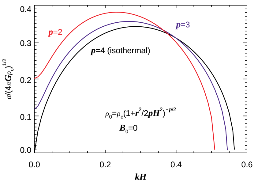
Similar to the isothermal model, the Plummer models of $p=2$ and 3 are unstable against fragmentation when the wavenumber is smaller than the critical one. The critical wavenumber, $k_{\rm cr}$, is smaller for a lower index, $p$, when measured in unit of $H^{-1}$. It is $k_{\rm cr}=0.509~{}H^{-1}$, $0.545~{}H^{-1}$ and $0.565~{}H^{-1}$ for $p$ = 2, 3, and 4, respectively. Also the wavenumber for which the growth rate takes its maximum value is also smaller for a lower index. However, it is premature to conclude that a filamentary cloud tends to fragment with a longer interval since the difference is small. We need to define the diameter of the filamentary cloud more carefully for obtaining before quantitative conclusion. It should be reminded that the radial density profile is broader for a lower $p$ when $\rho_{c}$ and $H$ are fixed. As shown in Figure 1, the diameter of $p=2$ model is slightly larger than that of $p=4$ if the filament diameter is defined as the full width at the half maximum.

The maximum growth rate, $\sigma_{\rm max}$, is higher for a lower, $p$, when measured in the unit of $\sqrt{4\pi G\rho_{c}}$. Again the dependence of $\sigma_{\rm max}$ on $p$ is weak. This is likely due to the fact that the cloud is more massive than the isothermal cloud when $\rho_{c}$ and $H$ are fixed, c.f., Equation (8).

Lowering the index induces radial collapse of the filament. When $p<4$, the model is unstable at $kH=0$, i.e., against radial collapse. This is because the effective sound speed decreases as the density increases. Remember that the critical line mass is $\lambda_{\rm cr}=2c_{s}^{2}/G$ for an isothermal filamentary to be sustained by gas pressure against collapse. The line mass of our equilibrium model is evaluated to be

$$\lambda_{\rm eq} = \frac{4\pi G\rho_{c}H^{2}}{p-2},$$ (66)

for $2<p<4$ from equation (8). Equation (66) means that the line mass is proportional to the square of the effective sound speed. Thus the radial collapse is stabilzed only when the effective sound speed increases as the density increases. Otherwise, the self-gravity overwhelms the gas pressure and the radial collapse sets in.

3.2 Case of $kH=0$

Figure 4 denotes the growth rate of the radial collapse ($kH=0$) mode, $\sigma/\sqrt{4\pi G\rho_{c}}$, as a function of the index, $p$, for $B_{0}=0$. It is obtained numerically with the method shown in Appendix B with the outer boundary at $r=200H$. The growth rate is lower for a higher $p$ and vanishes at $p=4$ (isothermal). It should be also noted we find only one unstable mode for a given $kH$.

Figure 4: Growth rate is shown as a function of the index, $p$, for for radial collapse, $k=0$ of the unmagnetized model ($B_{0}=0$).

This dependence of the instability on the equation of sate has been well known as summarized in the review by Larson (2003). Recently, Toci & Galli (2015a) have reported a similar result on the radial collapse of a filamentary cloud. They assumed the polytropic equation of state, $P=K\rho^{\gamma_{\rm p}}$, where $K$ and $\gamma_{\rm p}$ are a constant and the polytropic exponent, respectively. When $\gamma_{\rm p}<1$, their model cloud is also unstable against radial collapse. When $\gamma_{\rm p}>1$, the model cloud is stable against radial collapse and the density vanishes at a finite radius.

The dependence of the growth rate on the index, $p$, is moderate while it is larger for a lower $kH$. Thus we examine the eigenmode of the radial collapse for $p=2$ and 3. The upper panel of Figure 5 shows the relative density perturbation, $\delta\rho/\rho_{0}$, as a function of $r$ for the radial collapse mode, $kH=0$ and $B_{0}=0$. The lower panel of Figure 5 shows the radial displacement, $\xi_{r}/H$. The red curve denotes the eigenmode of $p=2$ while the black curve does that of $p=3$. The eigenmodes are normalized so that the relative density perturbation be unity, $\delta\varrho/\rho_{0}=1$. See Equations (20) and (21) for the definition of $\delta\varrho$ and its relation to the displacement.

Figure 5: The radial collapse mode is shown as a function of $r$. The upper panel shows the relative density perturbation while the lower one does the radial displacement. The red curves denote the eigenmode of $p=2$ while the black ones do those of $p=3$. The amplitude of the eigenmode is normalized so that $\delta\varrho/\rho_{0}=1$ at $r=0$.

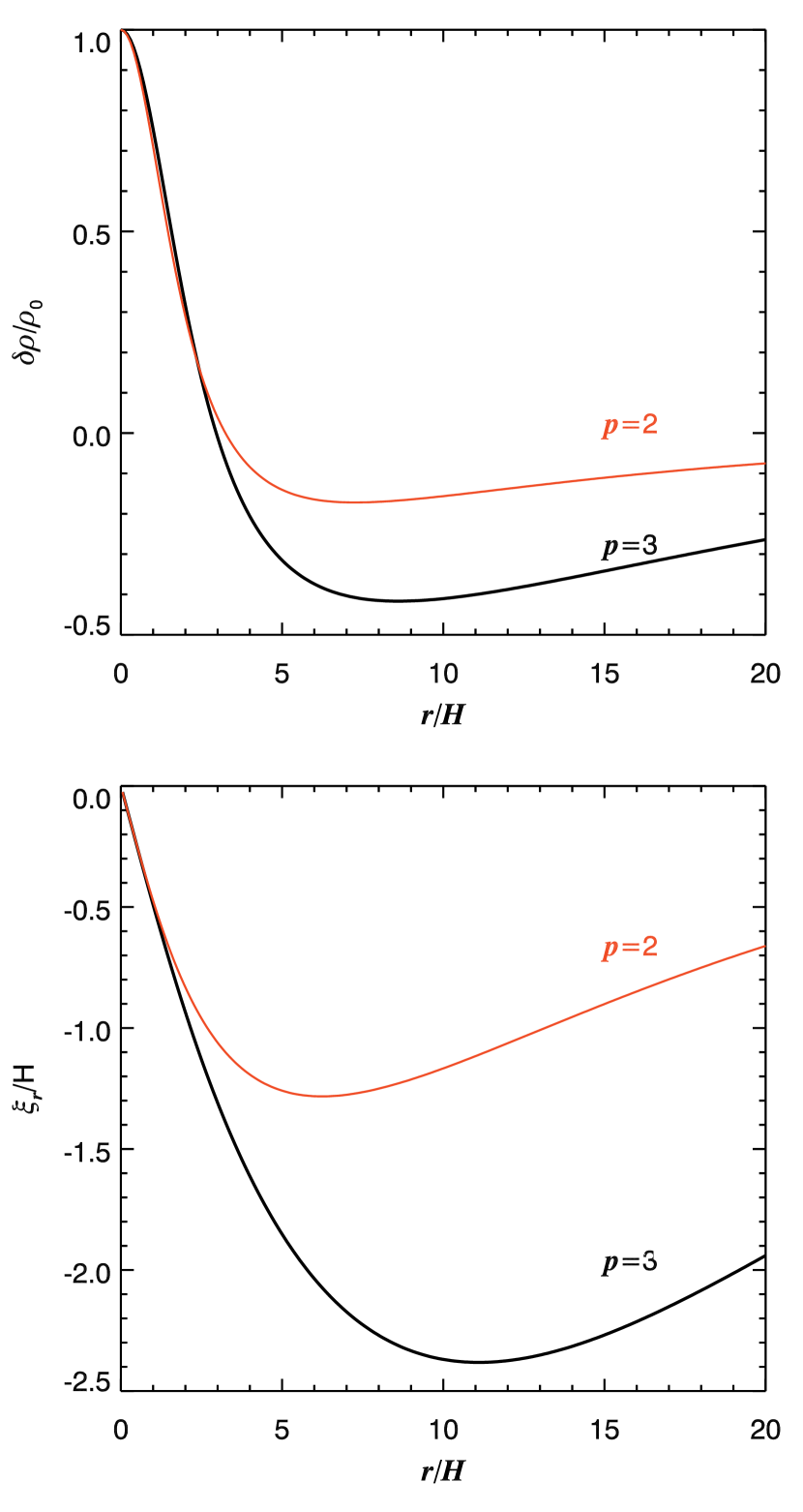
When the index is smaller than $p<4$, the effective equation of state is “soft” in a sense that the effective sound speed decreases as the density increases. Thus the filamentary cloud is subject to the radial collapse. When $p=2$ and 3, the radial displacement has a maximum at $r\simeq 5H$ and $11H$, respectively. When $p$ is small, an inner part region around the axis collapses radially. When $p$ is close to 4, the radial collapse is realized only when the whole cloud collapses in the radial direction.

The radial collapse ($kH=0$) is suppressed by a relatively weak magnetic field. Figure 6 shows the growth rate as a function of the inverse of the plasma beta, i.e., the magnetic pressure normalized by the gas pressure at the cloud center. The solid curves denote the growth rates for the free boundary, while the dashed ones those for the fixed boundary at $x=32H$. The index is set to be $p=$ 1.5, 2 and 3. Relatively weak magnetic field of $\beta_{\rm c}=5$ suppresses the $kH=0$ mode for $p=2$. When $p=3$, the radial collapse mode is completely suppressed by very weak magnetic field of $\beta_{\rm c}=40$.

Figure 6: The growth rate of $kH=0$ mode is shown as a function of $1/\beta_{\rm c}$ for $p=1.5$, 2, and 3. The solid curves denote those for the free boundary while the dashed ones those for the fixed boundary at $|x|=32H$.

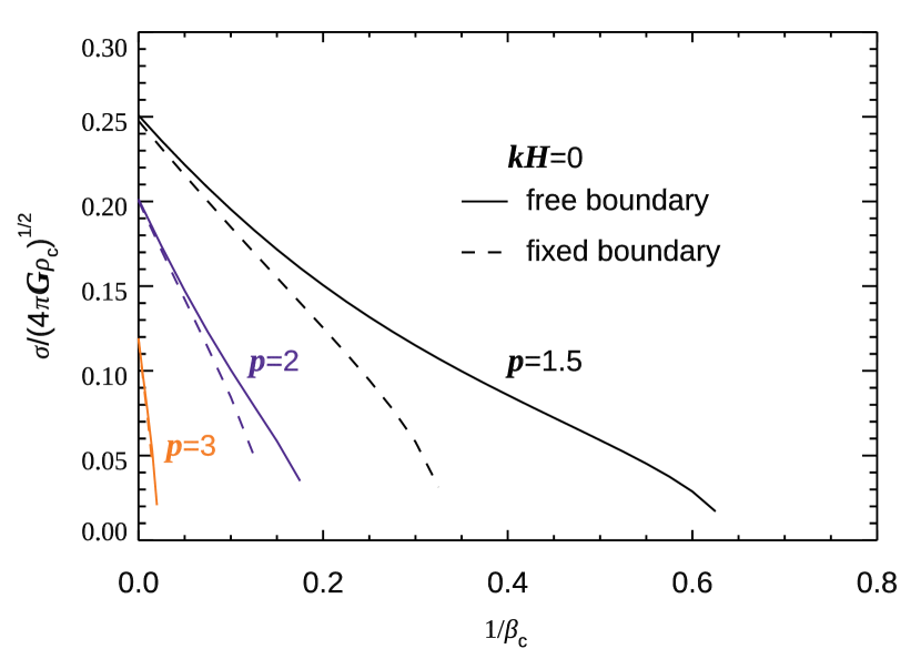
The magnetic field stiffens the equation of state since the magnetic pressure increases more steeply than the gas pressure when compressed. The radial collapse is thought to be suppressed when the equation of state is ’isothermal’ in effect, i.e., when the effective sound speed changes little by the increase in the density.

The growth is lower for given $p$ and $\beta$ when the fixed boundary condition is applied. When the magnetic field is fixed in the region far from the cloud, the magnetic tension works against the collapse in addition to the magnetic pressure. The difference is larger for a smaller $p$. The difference is negligibly small for $p$ = 3. When $p=2$, the difference is appreciable for $\beta<10$. The difference depends a little on the computation domain. The growth rate depends little on the size of the computation domain ($n_{x}$), when the free boundary is applied. However, the growth rate depends a little on $n_{x}$ when the fixed boundary is applied.

3.3 Case of $B_{0}\neq 0$ and $kH\neq 0$

First, we examine the case of $p=2$, since the density profile is close to the observed one.

Figure 7 denotes the growth rate, $\sigma/\sqrt{4\pi G\rho_{c}}$, as a function of the wave number, $kH$, for $p=2$ and the fixed boundary condition. Each curve denotes the growth rate for a given $B_{0}$. The label denotes the plasma beta on the cloud axis. Figure 7 is obtained with the spatial resolution, $\Delta x=\Delta y=0.4H$, the computation box size, $n_{x}=n_{y}=80$, and the wavelength resolution, $\Delta k=0.01H^{-1}$.

Figure 7: Growth rate, $\sigma$, is shown in unit of $\sqrt{4\pi G\rho_{\rm c}}$ as a function of the wavenumber, $kH$, for $p=2$ and the fixed boundary.

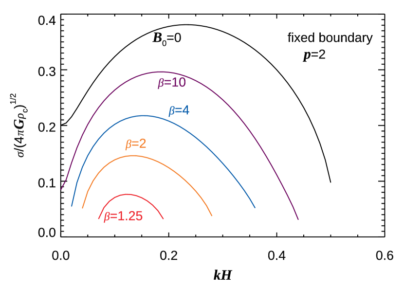
The growth rate is lower for a stronger magnetic field. When the initial magnetic field is uniform as assumed in our model, any perturbation increases magnetic energy. Hence, any perturbation induces restoring force proportional to the square of the magnetic field. The radial collapse is suppressed for $\beta<4$ since the magnetic field reduces the compressibility of the gas. The unstable mode is completely stabilized when $\beta<0.7$, while the entire cloud is subcritical for $\beta<0.203$ (see §2.1). This result is analogous to that in Paper I. The isothermal cloud is completely stabilized for $\beta<1.67$ while the entire cloud is subcritical for $\beta<0.405$.

The growth rate depends a little on the size of the computation domain, $n_{x}\Delta x$. The dependence on the domain size is appreciable when the growth rate is small. When $p=2$, $\beta=2.0$, $kH=0.2$ and $\Delta x=0.4~{}H$, the growth rate is 0.124 and 0.139 $\sqrt{4\pi G\rho_{c}}$ for $n_{x}=80$ and 120, respectively. The initial density is very low $\rho_{0}/\rho_{c}=3.89\times 10^{-3}$ and $1.73\times 10^{-3}$ at the numerical boundary at $32H$ and $48$, respectively. However, the location of the boundary affects the instability through the magnetic tension. When the magnetic field is fixed at a relatively short distance, the magnetic tension is strong enough to stabilize the cloud against fragmentation.

Figure 8 is the same as Figure 7 but for the free boundary. The growth rate is obtained with the same resolution, $\Delta x=\Delta y=0.4H$, $n_{x}=n_{y}=80$ and $\Delta k=0.01H^{-1}$. When $\beta<1$, the growth rate is well approximated by an empirical formula,

$$\sigma^{2}(k,\beta) = \sigma^{2}(k,0)+\frac{d\sigma^{2}}{d\beta}\beta+{\cal O}(\beta^{2}),$$ (67)

where $\sigma(k,0)$ and $d\sigma^{2}/d\beta$ are positive constants for a given $k$. The growth rate for $\beta=0$ shown in Figure 8 is obtained by the linear extrapolation of the growth rates at $\beta=0.1$ and 0.5.

Figure 8: The same as Fig. 7 but for the free boundary.

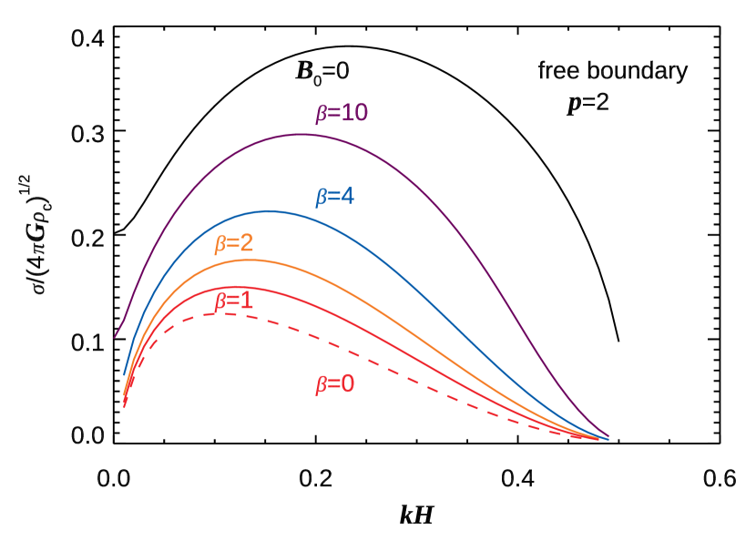
The growth rate depends little on the size of the computation domain. When $p=2$, $\beta=2$, $kH=0.2$ and $\Delta x=0.4H$, the growth rate is 0.160 and 0.161 $\sqrt{4\pi G\rho_{c}}$ for $n_{x}=80$ and 120, respectively.

The growth rate is lower for a stronger magnetic field also when the free boundary is applied. The radial collapse is suppressed by a mildly strong magnetic field ($\beta<4$). However, the model cloud is unstable against fragmentation even when the entire cloud is subcritical. This instability is due to rearrangement of magnetic flux tubes as shown in paper I. Although the critical wavenumber changes little, the wavenumber of the most unstable mode decreases down to $(kH)_{\rm max}\simeq 0.11$ in the limit of $\beta=0$.

Comparison of Figures 7 and 8 tells us that the growth rate depends significantly on the boundary condition only when $\beta\lesssim 2$. When the gas pressure dominates over the magnetic pressure on the cloud axis ($\beta\gtrsim 2$), the growth rate is nearly the same for both the free and fixed boundaries except for $kH\lesssim 0.4$, i.e., when the wavenumber is close to $k_{\rm cr}$ and the instability is weak even for $B_{0}=0$. This means that a relatively weak magnetic field does not play an important role in the region far from the axis, although the magnetic pressure dominates over the gas pressure thereof. Remember that the magnetic pressure is comparable to the gas pressure at $r=12H$ even when the $\beta=10$. The gas pressure decreases with the decrease in the density while the magnetic pressure remains constant in our model. The magnetic pressure dominates over the gas pressure near the outer boundary ($x=32H$ and $y=32H$) of our numerical computation even for $\beta=100$. The magnetic field can suppress the fragmentation only when the magnetic field is strong near the cloud axis and fixed in the region very far from the cloud.

The Plummer index, $p$, can vary from cloud to cloud. Thus we examine two cases, $p=1.5$ and $p=3$. The former is close to the observed minimum.

Figures 9 and 10 show the growth rate, $\sigma/\sqrt{4\pi G\rho_{c}}$, as a function of the wavenumber, $kH$, for the model of $p=1.5$. Figure 9 denotes the growth rate for the fixed boundary while Figure 10 does that for the free boundary. The results are qualitatively similar to those for $p=2$, while the growth rate is a little larger for given $kH$ and $\beta$. As a result, the model cloud is unstable against fragmentation for $\beta=1$ even when the fixed boundary is applied. The growth rate depends significantly on the boundary condition when $\beta\lesssim 1$.

The increase in the growth rate might be due to the normalization. The growth rate is normalized by the initial central density ($\rho_{c}$). The wavenumber is normalized not only by the density but by the sound speed ($\sqrt{dP/d\rho}$) on the cloud axis, since the unit length can be expressed as

$$H = \frac{1}{\sqrt{8\pi G\rho_{c}}}\left[\frac{dP_{0}}{d\rho_{0}}\left(\rho_{c}\right)\right]^{1/2}.$$ (68)

Equation (68) is derived from Equations (13) and (14) by taking the limit of $r\rightarrow 0$. In other words, the growth rate is normalized by the free-fall timescale at the cloud center, while the wavenumber is normalized by the Jeans length, $\lambda_{\rm J}=2\pi H$. When the central density and sound speed are fixed, the mass per unit inside radius, $r$, is larger for a smaller $p$. The increase in the growth rate is likely to be ascribed to the increase in the mass per unit length since this instability is due to the self-gravity.

Figure 9: The same as Figure 7 but for $p=1.5$ and the fixed boundary.

Figure 10: The same as Fig. 8 but for $p=1.5$ and the free boundary.

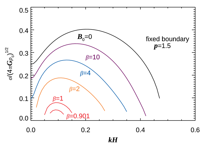
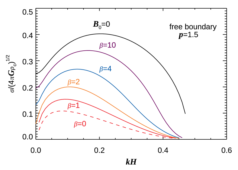
Figures 11 and 12 are the same as Figures 7 and 8 but for $p=3$, respectively. The result depends only quantitatively on $p$ as expected. The growth rate is intermediate between those for $p=2$ and 4. When the fixed boundary is applied, the cloud is stabilized by a moderately strong magnetic field ($\beta\lesssim 1.3$). The radial collapse ($kH\ll 0.05$) mode is suppressed by a relatively weak ($\beta\approx 10$) magnetic field.

Figure 11: Growth rate is shown as a function of the wavenumber for $p$ = 3. The fixed boundary condition is applied.

Figure 12: The same as Fig. 11 but for the free boundary.

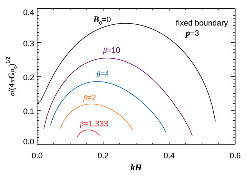
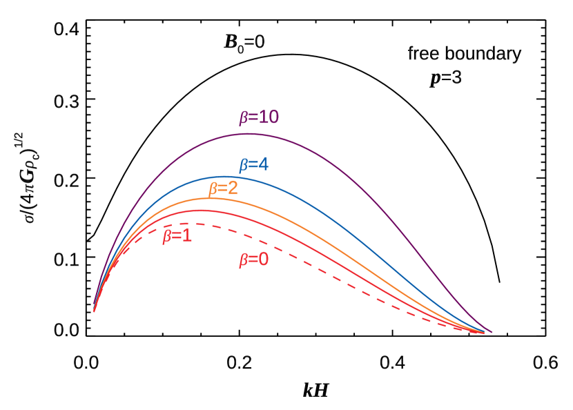
The eigenfunction depends only weakly on the index, $p$. We do not find any qualitative change except for the radial collapse in case of weak magnetic field.

4 DISCUSSIONS

First we compare our equilibrium model clouds with earlier theoretical models based on effective equation of state.

Ostriker (1964) obtained cylindrical equilibrium models by assuming polytropic equation of state,

$$P = K_{N}\rho^{1+1/N},$$ (69)

where $K_{N}$ and $N$ denotes the polytropic constant and index, respectively. His equilibrium model is symmetric around the axis and extended infinitely along the axis. Since he studied the case of $N\geq 1$, the effective sound speed, $\left(dP/d\rho\right)^{1/2}$, increases as the density increases. In his model, the model cloud is truncated at a certain radius when $N$ is finite. Only when $N$ is infinite (isothermal), the cloud is extended to an infinite radius.

When $N$ is negative, the polytrope gives a similarity solution denoting radial collapse (McLaughlin & Pudritz, 1997; Kawachi & Hanawa, 1998). The density decreases in proportion to

$$\rho \propto r^{-2/(1-1/N)},$$ (70)

in the region far from the cloud axis. This radial profile is quite similar to the Plummer-like model with $p\simeq 2$, when $N$ is negatively large.

McLaughlin & Pudritz (1997) introduced a model with a slightly different equation of state, Equation (15), which is named ‘logatrope’. The sound speed is inversely proportional to the density as shown in Equation (16). The polytrope gives a singular equilibrium having the density profile, $\rho\propto r^{-1}$. This corresponds to the polytrope model of $N=-1$.

Note that the polytropic equation of state has a steeper dependence on the density compared with our model equation of state. The sound speed is proportional to a power of the density, $dP/d\rho\propto\rho^{1/N}$. Our model equation of state shows further weaker dependence of the sound speed on the density as shown in Figure 2. Note that the effective sound speed is only 2.16 and 1.28 times at $\rho=\rho_{c}/100$ than that at $\rho=\rho_{c}$ for $p=2$ and 3, respectively. The small change produces notable change in the radial density profile. We introduced this effective sound speed by taking account of the turbulence, but physical change in the temperature may contribute to density profile. It should be noted that exactly and almost isothermal models give different radial density profiles for the equilibrium.

When the effective sound speed decreases with increase in the density, the cloud is unstable against radial collapse. Our analysis indicates that the radial collapse can be suppressed by magnetic field perpendicular to the cloud, if they are appreciable. The conclusion is likely to be valid in general.

Our analysis indicates that perpendicular magnetic field affects the dynamics of a filamentary cloud when the plasma beta is close to unity. The plasma beta can be evaluated from the effective sound speed ($c_{\rm s,eff}$), the filament width ($w$), and the magnetic field, $B_{0}$. if the filamentary cloud is supported by pressure, the filament mass per unit length is evaluated to be

$$\lambda \approx \frac{2c_{\rm s,eff}^{2}}{G}.$$ (71)

Then the gas pressure at the cloud center is evaluated to be

$$P_{\rm c} \approx \frac{4c_{\rm s,eff}^{2}\lambda}{\pi w^{2}}.$$ (72)

Thus the plasma beta is evaluated to be

$$\beta \approx \left(\frac{c_{\rm s,eff}}{0.3~{}\mbox{km~{}s}^{-1}}\right)^{4}\left(\frac{w}{0.1~{}\mbox{pc}}\right)^{-2}\left(\frac{B_{0}}{90~{}\mu\mbox{G}}\right)^{-2}.$$ (73)

Equation (73) implies magnetic field of $\sim 100~{}\mu$G plays an important role in the dynamics of a typical molecular cloud, since the numbers quoted are typical. The plasma beta can be evaluated also from $w$ and $\lambda$, if Equation (71) is valid.

It is interesting to apply the above estimate to the Musca filamentary cloud. The central 1.6 pc of the filamentary cloud shows no sign of fragmentation, although the rest of the cloud shows fragmentation consistent with stability analysis (Kainulainen et al., 2016). If the stabilization is due to perpendicular magnetic field, the field strength should be several tens $\mu$G. According to Kainulainen et al. (2016), the best fit Plummer model gives $p$ = 2.6 and 1.8 in the west and east sides of the filamentary cloud, respectively. They also evaluate the effective sound speed to be 22 % higher than the isothermal one. The right hand side of Equation (73) is roughly unity when $B_{0}\approx 100~{}\mu\mbox{G}$.

Our stability analysis has demonstrated that the instability depends on the boundary condition, i.e., fixed or free, when the plasma beta is close to unity. This means that a filamentary cloud is not isolated and the stability depends on the environment. This suggests an interesting possibility. If two filamentary clouds are threaded by the same perpendicular magnetic field lines, their fragmentation can be linked through magnetic force. Fragmentation of a cloud might be suppressed since the magnetic field lines are fixed by the other cloud. However, we cannot exclude the possibility that two clouds fragment coherently. This problem is beyond the scope of this paper and an open question.

Except for the radial collapse, the growth rate of the perturbation depends only quantitatively on the index, $p$. Any strong magnetic field cannot stabilize the cloud if the magnetic fields are free to move in the region far from the cloud. However, this does not mean that a filamentary cloud fragment to form cores in a short timescale. The growth rate is nearly by a factor of ten smaller than the dynamical one, $\sqrt{4\pi G\rho_{c}}$, for $p=2$ as shown in Figure 8. Remember that the growth rate is normalized by the free-fall timescale at the cloud center,

$$\tau_{\rm ff}\;=\;\frac{1}{\sqrt{4\pi G\rho_{c}}} = 0.18~{}\left(\frac{n_{{\rm H}_{2}}}{10^{4}~{}\mbox{cm}^{-3}}\right)^{-1/2}~{}\mbox{Myr}.$$ (74)

Since the growth rate is small, we need to take account of non-ideal effects, i.e., the ambipolar diffusion of magnetic field, which is ignored in our analysis for simplicity. It is well known that the ambipolar diffusion increases mass to flux ratio locally and makes a molecular cloud eventually supercritical. This competing process should be taken account seriously, if we discuss the instability due to the rearrangement of magnetic flux tubes.

We also note that the growth rate of the rearrangement instability is smaller for a smaller, $p$, although the maximum growth rate of $B_{0}=0$ is larger for a smaller $p$. This result is consistent with the discussion given in paper I. Rearrangement of magnetic fields travel along the field line as the Alfvén wave, which is proportional to $B_{0}/\sqrt{\rho_{0}}$. Thus the rearrangement takes more times when either magnetic field weakens or the density decreases more slowly in the region far from the cloud. In our analysis, only the latter effect is taken into account, while the magnetic fields should be weaker outside the cloud than inside. Thus the rearrangement instability grows more slowly if non-uniformity of magnetic field is taken account.

5 Summary

We have examined the stability of filamentary cloud permeated by uniform perpendicular magnetic fields with a focus on the dependence on the initial density. Our main findings are summarized as follows.

1. The observed Plummer-like density profile can be realized if the effective sound speed increases with decrease in the density. The radial density slope is $d\ln\rho/d\ln r=-2$, if the effective sound speed is only by a factor of 5 larger in the region where the density is by a factor of 100 lower than at the cloud center. This dependence of the effective sound speed on the density is much lower than that of a logatrope.

2. When the radial density slope is shallower than $d\ln\rho/d\ln r>-4$, the cloud is unstable against radial collapse. The growth rate is larger when the radial density slope is shallower. The radial collapse can be suppressed by mildly strong magnetic fields.

3. Stability of a filamentary cloud depends strongly on the boundary condition far from the filament, i.e., on the environment. If the magnetic field is fixed at a large distance from the cloud and the plasma beta is close to unity at the center of the cloud, fragmentation is suppressed. If the magnetic field line can move freely, it cannot suppress the fragmentation even when the cloud is magnetically subcritical. The latter instability is induced by rearrangement of magnetic flux tubes as shown in Paper I.

Appendix A Boundary Condition for the Poisson Equation

We improved the boundary condition for the Poisson equation. Equation (42) relates the change in the gravitational potential to that in the density, where the Green’s function, $G_{i,j,i^{\prime},j^{\prime}}$, takes account of the boundary conditions on $x=0$ and $y=0$. In this work we removed the boundary by employing the method of the mirror image, i.e., by taking account of the change in the density in the regions of $x<0$ and/or $y<0$. Then the boundary conditions for the Poisson equations are expressed as

$$\lim_{\sqrt{x^{2}+y^{2}}\rightarrow\infty}\left|\mbox{\boldmath$\phi$}\right|=0.$$ (A1)

The corresponding Green’s function is expressed as

$$G^{\prime}_{i,j,i^{\prime},j^{\prime}} = 2G\Delta x\Delta yK_{0}(kr),$$ (A2)

$$r = \sqrt{\left(i-i^{\prime}\right)^{2}\Delta x^{2}+\left(j-j^{\prime}\right)^{2}\Delta y^{2}},$$ (A3)

where $K_{0}$ denotes the 0-th modified Bessel function of the second kind and the argument is the distance from the source multiplied by the wavenumber, $k$. We solved the discretized Poisson equation,

$$\frac{G^{\prime}_{i+1,j,0,0}-2G^{\prime}_{i,j,0,0}+G^{\prime}_{i-1,j,0,0}}{\Delta x^{2}}+\frac{G^{\prime}_{i,j+1,0,0}-2G^{\prime}_{i,j,0,0}+G^{\prime}_{i,j-1,0,0}}{\Delta y^{2}}-k^{2}G^{\prime}_{i,j,0,0} = \begin{cases}1&(i=j=0)\\ 0&\mbox{(otherwise)}\end{cases},$$ (A4)

with boundary condition (A2), on $i=\pm(3n_{x}+1)$ and $j=\pm(3n_{y}+1)$ by the Gauss-Seidel iteration. Once the Green’s function, $G^{\prime}_{i,j,0,0}$, is given, then the Green’s function, $G_{i,j,i^{\prime},j^{\prime}}$, is obtained by summing up the contributions from the mirror images. Thus we can save the computation time for solving the Poisson equation greatly by the method of mirror image. The boundary condition (A2) improves the accuracy of the Green’s function for a small wavenumber, $kH\lesssim 0.05$.

When $k=0$, Eq. (A2) is replaced with

$$G^{\prime}_{i,j,i^{\prime},j^{\prime}} = -2G\Delta x\Delta y\ln r,$$ (A5)

where the asymptotic form of the modified Bessel function near $z=0$ is applied. Although Equation (A5) contains an offset proportional to $\ln(k/2)$, the $x$- and $y$-components of the gravity are not affected by the offset.

Appendix B Case of $B_{0}=0$

When $B_{0}=0$, our equilibrium model is symmetric and the perturbation equation is reduced to an ordinary differential equation if we use the cylindrical coordinate, $(r,\varphi,z)$. Following Appendix C of paper I, we express the density, displacement and potential in the form,

$$\rho = \rho_{0}+\delta\varrho(r)\cos kz,$$ (B1)

$$\xi = \xi_{r}(r)\cos kz\mbox{\boldmath$e$}_{r}+\xi_{z}(r)\sin kz\mbox{\boldmath$e$}_{z},$$ (B2)

$$\psi = \psi_{0}+\delta\psi(r)\cos kz.$$ (B3)

The perturbation equations are written as

$$\delta\varrho = -\frac{1}{r}\frac{\partial}{\partial r}\left(r\rho_{0}\xi_{r}\right)-k\rho_{0}\xi_{z},$$ (B4)

$$\sigma^{2}\xi_{r} = -\frac{\partial}{\partial r}\left[\left(\frac{dP}{d\rho}\right)\frac{\delta\varrho}{\rho_{0}}\right]-\frac{\partial}{\partial r}\delta\psi,$$ (B5)

$$\sigma^{2}\xi_{z} = k\left(\frac{\partial P}{\partial\rho}\right)\frac{\delta\varrho}{\rho_{0}}+k\delta\psi,$$ (B6)

$$4\pi G\delta\varrho = \frac{1}{r}\frac{\partial}{\partial r}\left(r\frac{\partial}{\partial r}\delta\psi\right)-k^{2}\delta\psi.$$ (B7)

From Equations (B5) and (B6), we obtain

$$\xi_{z} = -\int k\xi_{r}dr.$$ (B8)

We solve Equations (B4), (B5), (B7), and (B8) in the discretized form.

We express the perturbation using the radial displacement, $\mbox{\boldmath$\xi$}_{r}=(\xi_{r,1/2},\xi_{r,3/2},\dots,\xi_{r,n-1/2})$, where $\xi_{r,j-1/2}$ denotes the radial displacement at $r=(j-1/2)\Delta r$. We will show that Equation (B5) can be expressed in the discretized form,

$$\sigma^{2}\xi_{r,j-1/2} = \sum_{i}F_{ji}\xi_{r,i-1/2},$$ (B9)

where the matrix elements, $F_{ji}$, are obtained by the following procedure. When evaluating $F_{ji}$, we set

$$\xi_{r,j-1/2} = \begin{cases}1&\mbox{if}~{}j=i\\ 0&\mbox{otherwise}\end{cases}.$$ (B10)

Using equation (B8) we obtain the longitudinal displacement,

$$\xi_{z,j} = \begin{cases}-k\Delta r&(j<i)\\ 0&j\geq i\end{cases}.$$ (B11)

The change in the density is evaluated to be

$$\delta\varrho_{j} = \begin{cases}\displaystyle-\frac{4\rho_{0,1/2}\xi_{r,1/2}}{\Delta r}-k\rho_{0,0}\xi_{z,0}&(j=0)\\ \displaystyle-\frac{1}{r_{j}\Delta r}\left(r_{j+1/2}\rho_{0,j+1/2}\xi_{r,j+1/2}-r_{j-1/2}\rho_{0,j-1/2}\xi_{r,j-1/2}\right)-k\rho_{0,j}\xi_{z,j}&(j\neq 0)\end{cases},$$ (B12)

by discretizing Equation (B4), where $\delta\varrho_{j}$ and $\rho_{0,j+1/2}$ denote the values at $r=r_{j}$ and $r_{j+1/2}$, respectively. The change in the gravitational potential, $\delta\psi$, is obtained by solving the discretized Poisson equation

$$4\pi G\delta\varrho_{j} = \left\{\begin{array}[]{ll}\displaystyle 2\frac{\delta\psi_{1}-\delta\psi_{0}}{\Delta r^{2}}-k^{2}\delta\psi_{0}&\hskip 20.0pt(j=0)\\ \displaystyle-\frac{r_{j+1/2}\delta\psi_{j+1}-2r_{j}\delta\psi_{j}+r_{j-1/2}\delta\psi_{j-1}}{r_{j}\Delta r^{2}}-k^{2}\delta\psi_{j}&\hskip 20.0pt(j=1,2,\dots,n)\end{array}\right.,$$ (B15)

with the boundary condition

$$\delta\psi_{n+1}=\frac{K_{0}[k(n+1)\Delta r]}{K_{0}(kn\Delta r)}\delta\psi_{n},$$ (B16)

where $K_{0}$ denotes the modified Bessel function (see Appendix A). By discretizing Equation (B5) we obtain

$$\sigma^{2}\xi_{r,j-1/2} = -\frac{1}{\Delta r}\left[\left(\frac{dP}{d\rho}\right)_{j}\frac{\delta\varrho_{j}}{\rho_{0,j}}-\left(\frac{dP}{d\rho}\right)_{j-1}\frac{\delta\varrho_{j-1}}{\rho_{0,j-1}}+\delta\psi_{j}-\delta\psi_{j-1}\right].$$ (B17)

The righthand side of Equation (B17) denotes the matrix element, $F_{ji}$.

When $k=0$, we replace Equation (B17) with

$$\sigma^{2}\xi_{r,j-1/2} = \displaystyle-\frac{1}{\Delta r}\left[\left(\frac{dP}{d\rho}\right)_{j}\frac{\delta\varrho_{j}}{\rho_{0,j}}-\left(\frac{dP}{d\rho}\right)_{j-1}\frac{\delta\varrho_{j-1}}{\rho_{0,j-1}}\right]+4\pi G\rho_{0,j}\delta_{i,j}$$ (B18)

where $\delta_{i,j}$ denotes the Kronecker’s delta, since

$$\frac{\partial\psi}{\partial r} = -4\pi G\rho_{0}\xi_{r}$$ (B19)

for $k=0$.

The growth rate, $\sigma$, is obtained as the eigenvalue of the matrix, $F_{ji}$. The spatial resolution and outer boundary are set to be $\Delta r=0.1H$ and $r_{n}\geq 60H$. The outer boundary should be set very far $(r\geq 100H)$ for $p<1$. Otherwise the growth rate is underestimated.

References

- Anderson et al. (1999) Anderson, E., Bai, Z., Bischof, C., Blackford, S., Demmel, J., Dongarra, J., Du Croz, J., Greenbaum, A., Hammarling, S., McKenney, A., Sorensen, D. 1999, LAPACK Users’ Guide, 3rd ed. http://www.netlib.org/lapack/lug/
- André et al. (2014) André P., Di Francesco J., Ward-Thompson D. 2014 Protostars and Planets VI ed H. Beuther et al. (Tucson, AZ: Univ. Arizona Press) 27
- Arzoumanian et al. (2011) Arzoumanian, D., André, Ph., Didelon, P. et al. 2011, A&A, 529, L6
- Fiege & Pudritz (2000) Fiege, J.D., Pudritz, R.E. 2000, MNRAS, 311, 105
- Hanawa et al. (1993) Hanawa T., Nakamura F., Matsumoto, T., et al. 1993, ApJ, 404, L83
- Hanawa & Tomisaka (2015) Hanawa, T., Tomisaka, K. 2015 ApJ 801 11
- Hanawa, Kudoh & Tomisaka (2017) Hanawa, T., Kudoh, T., Tomisaka, K. 2017, ApJ, 848, 2 (paper I)
- Hosseinirad et al. (2018) Hosseinirad, M., Abassi, S., Roshan, M., Naficy, K. 2018, MNRAS, 475, 2632
- Juvela et al. (2012) Juvela, M. et al. 2012, å, 541, A12
- Kainulainen et al. (2016) Kainulainen, J., Hacer, A., Alves, J., Beuther, H., Bouy, H., Taffala, M. 2016, A&A, 586, A27
- Kawachi & Hanawa (1998) Kawachi, T., Hanawa, T. 1998, PASJ, 50, 577
- Kusune et al. (2016) Kusune, T., Sugitani, K., Nakamura, F. et al. 2016, ApJ, 830, L23
- Larson (2003) Larson R. B. 2003 RPPh, 66, 1651
- McLaughlin & Pudritz (1996) McLaughlin, D.E., Pudritz, R.E. 1996, ApJ, 469, 164
- McLaughlin & Pudritz (1997) McLaughlin, D.E., Pudrltz, R.E. 1997, ApJ, 476, 750
- Nagai, Inutsuka & Miyama (1998) Nagai T., Inutsuka S.,Miyama S.M. 1998, ApJ, 506, 306
- Nakamura, Hanawa & Nakano (1993) Nakamura, F., Hanawa, T., Nakano, T. 1993, PASJ, 45, 551
- Nakano & Umebayashi (1988) Nakano, T., Umebayashi, T. 1988, Prog. Theor. Phys. Suppl., 96, 73
- Ohashi et al. (2018) Ohashi, S., Sanchueza, P., Sakai, N. et al. ApJ, 856, 147
- Ostriker (1964) Ostriker, J. 1964, ApJ, 140, 1056
- Palmeirim et al. (2013) Palmeirim P., André P., Kirk J. et al. 2013, A&A, 550, A38
- Stodólkiewicz (1963) Stodólkiewicz, J.S. 1963, Acta Astron., 13, 30
- Soler et al. (2016) Soler, J.D., Alves, F., Boulanger, E. et al. 2016, A&A, 596, A93
- Sugitani et al. (2011) Sugitani K., Nakamura F., Watanabe M. et al. 2011 ApJ, 734, 63
- Toci & Galli (2015a) Toci, C., Galli, D. 2015a, MNRAS, 446, 2110
- Toci & Galli (2015b) Toci, C., Galli, D. 2015b, MNRAS, 446, 2118
- Tomisaka (2014) Tomisaka, K. 2014, ApJ, 785, 24