The operator product expansion (OPE), truncated in dimension, is employed in many contexts. An example is the extraction of the strong coupling, $\alpha_{s}$, from hadronic $\tau$-decay data, using a variety of analysis methods based on finite-energy sum rules. Here, we reconsider a long-used method, which parametrizes non-perturbative contributions to the $I=1$ vector and axial vacuum polarizations with the OPE, setting several higher-dimension coefficients to zero in order to implement the method in practice. The assumption that doing this has a negligible effect on the value of $\alpha_{s}$ is tantamount to the assumption that the low-dimension part of the OPE converges rapidly with increasing dimension near the $\tau$ mass. Were this assumption valid, it would certainly have to be valid at energies above the $\tau$ mass as well. It follows that the method can be tested using data obtained from $e^{+}e^{-}\to\mbox{hadrons}$, as they are not limited by the kinematic constraints of $\tau$ decays. We carry out such an investigation using a recent high-precision compilation for the $R$-ratio, arguing that it provides insights into the validity of the strategy, even if it probes a different, though related channel. We find that $e^{+}e^{-}$-based tests call into question the implied assumption of rapid convergence of the low-dimension part of the OPE around the $\tau$ mass, and thus underscore the need to restrict finite-energy sum-rule analyses to observables which receive only contributions from lower-order terms in the OPE.

I Introduction

As is well known, the spectral function, $\rho_{\rm EM}(s)$, of $\Pi_{\rm EM}$, the scalar polarization of the electromagnetic (EM) current-current two-point function, is directly obtainable from the experimentally measured $R$-ratio,

$$R(s)\equiv{\frac{3s}{4\pi\alpha^{2}}}\,\sigma_{e^{+}e^{-}\to{\rm hadrons}(\gamma)}(s)={\frac{\sigma_{e^{+}e^{-}\to{\rm hadrons}(\gamma)}(s)}{\sigma_{e^{+}e^{-}\to\mu^{+}\mu^{-}}(s)}}\ ,$$ (1)

via

$$\rho_{\rm EM}(s)={\frac{1}{\pi}}\,\mbox{Im}\,\Pi_{\rm EM}(s)={\frac{1}{12\pi^{2}}}\,R(s)\ ,$$ (2)

where, in Eq. (1), $\alpha$ is the fine-structure constant, the second of the equations holds for values of $s$ for which the muon mass can be neglected, and the $\gamma$ in parentheses indicates that the hadronic states in question are inclusive of final-state radiation.

Similarly, information on the spectral functions, $\rho^{(J)}_{V/A;ij}(s)$, of the spin $J=0,\,1$ scalar polarizations, $\Pi_{ij;V/A}^{(J)}$, of the flavor $ij=ud$ and $us$ vector (V) and axial vector (A) current-current two-point functions can be obtained from the experimental hadronic $\tau$-decay distributions, $dR_{V/A;ij}/ds$. Explicitly tsai71 ,

$${\frac{dR_{V/A;ij}(s;s_{0})}{ds}} = {\frac{12\pi^{2}|V_{ij}|^{2}S_{\rm EW}}{s_{0}}}\,\left[w_{\tau}(y_{\tau})\rho_{V/A;ij}^{(0+1)}(s)-w_{L}(y_{\tau})\rho_{V/A;ij}^{(0)}(s)\right]\ ,$$ (3)

where $y_{\tau}=s/m_{\tau}^{2}$,

$$w_{\tau}(y) = (1-y)^{2}(1+2y)\ ,$$ (4)

$$w_{L}(y) = 2y(1-y)^{2}\ ,$$

$S_{\rm EW}$ is a known short-distance electroweak correction erler , $V_{ij}$ is the flavor $ij$ CKM matrix element and $dR_{V/A;ij}(s;s_{0})/ds$ is related to the total inclusive hadronic $\tau$-decay width by

$$R_{V/A;ij}(s_{0}) = \int_{0}^{s_{0}}ds\,{\frac{dR_{V/A;ij}(s;s_{0})}{ds}}\ ,$$ (5)

$$R_{V/A;ij}(m_{\tau}^{2}) = \frac{\Gamma[\tau^{-}\rightarrow\nu_{\tau}\,{\rm hadrons}_{V/A;ij}\,(\gamma)]}{\Gamma[\tau^{-}\rightarrow\nu_{\tau}e^{-}{\bar{\nu}}_{e}(\gamma)]}\ .$$

The analyticity properties of current-current polarizations (denoted generically by $\Pi$) ensure the validity of finite-energy sum rules (FESRs), which allow one to relate weighted integrals over the associated experimental spectral data to theoretical representations of the polarizations fesrrefs . Explicitly, for any $\Pi(s)$ free of kinematic singularities, any $s_{0}>0$, and any $w(s)$ analytic inside and on the contour $|s|=s_{0}$, one has the sum rule

$$I_{w}^{\rm exp}(s_{0})=I_{w}^{\rm th}(s_{0})\ ,$$ (6)

where the weighted integrals over the experimental spectral function and over the vacuum polarization are defined as

$$I_{w}^{\rm exp}(s_{0}) = \frac{1}{s_{0}}\int_{0}^{s_{0}}\,ds\,w\left(\frac{s}{s_{0}}\right)\,\rho(s)\ ,$$ (7a)

$$I_{w}^{\rm th}(s_{0}) = -{\frac{1}{2\pi is_{0}}}\,\oint_{|s|=s_{0}}ds\,w\left(\frac{s}{s_{0}}\right)\,\Pi(s)\ .$$ (7b)

For sufficiently large $s_{0}$, $I_{w}^{\rm th}(s_{0})$ can be approximated using the operator product expansion (OPE) for $\Pi$. This allows quantities entering the OPE (such as the strong coupling $\alpha_{s}$, quark masses, and effective higher-dimension vacuum condensates) to be related to experimental data, in principle. FESRs based on $ud-us$ flavor-breaking differences of hadronic $\tau$-decay distributions can also be used to provide an independent determination of $|V_{us}|$ gamizfbfesrvus ; kmcwfbfesrvus ; hlmz17 . Generalizing Eq. (6) to weights $w(s)/s^{N}$, still with $w(s)$ analytic, yields analogous inverse-moment FESR (IMFESR) relations involving quantities such as $\Pi(0)$, and its derivatives with respect to $s$ at $s=0$, which can be exploited to determine some of the low-energy constants of chiral peturbation theory (ChPT), provided those terms in the associated OPE required for the $w(s)$ chosen are known from external sources IMFESR . The OPE thus plays an important role in FESR and IMFESR analyses.

Information on the flavor $ud$, $us$ $V$ and $A$ spectral functions from hadronic $\tau$-decay data is, of course, only available up to the kinematic limit, $s=m_{\tau}^{2}$, restricting FESRs and IMFESRs based on hadronic $\tau$-decay data to $s_{0}\leq m_{\tau}^{2}$. No such kinematic limit exists for FESRs and IMFESRs based on hadronic electroproduction cross-section data.

The OPE is expected to provide an accurate representation of $\Pi(s)$ valid for Euclidean $Q^{2}\,\equiv\,-s\gg\Lambda_{\rm QCD}^{2}$, up to small exponentially suppressed corrections. In Eq. (7b), the OPE representation, however, must be used over the whole of the contour $|s|=s_{0}$, which includes the region near the Minkowski axis, where, as anticipated in Ref. pqw , the OPE breaks down at intermediate (timelike) $s$. This is clear from the presence of resonance peaks in experimental spectral functions at $s$ of order a few GeV². Such “duality violating” (DV) effects are expected to be localized to the vicinity of the Minkowski axis, an expectation confirmed by studies of FESRs employing both “unpinched” weights (those which do not vanish at $s=s_{0}$ and hence do not suppress contributions from the region near the Minkowski axis) and “pinched” weights (those with $w(s_{0})=0$, which do suppress contributions from that region) kmpinching . Precision determinations of $\alpha_{s}$, quark masses, and other OPE parameters may, however, require small residual DV contributions to be taken into account, even for FESRs involving pinched weights CGP ; alphas1 .

A second, related issue for the use of the OPE in FESRs and IMFESRs is the fact that the OPE (an expansion in $z=1/Q^{2}$) is not convergent BCGMP . Convergence would require the existence of a region in the complex plane around $z=0$ free of singularities, and hence, in the case of a current-current two-point function, the vanishing of the corresponding spectral function above some maximum value of $s$. This is not the case. The OPE is thus, at best, an asymptotic expansion, and one cannot safely assume that effective condensates $C_{D}$, of dimension $D$, defined by

$$\Pi_{\rm OPE}(-Q^{2})=\sum_{k=0}^{\infty}\frac{C_{2k}(Q^{2})}{(-Q^{2})^{k}}\ ,$$ (8)

naively scale as $\Lambda_{\rm QCD}^{D}$.

This is relevant for FESRs and IMFESRs employing weights $w(s)$ which generate OPE contributions proportional to higher dimension $C_{D}$ not known from external sources. Assumptions based on naive scaling of the $C_{D}$ have often been used to argue that such unknown contributions are “safely” negligible at scales of a few GeV², including $s_{0}\sim m_{\tau}^{2}$. In general, a polynomial weight $w(y)=\sum_{k=0}^{N}b_{k}y^{k}$, $y=s/s_{0}$, produces, up to logarithmic corrections suppressed by additional powers of $\alpha_{s}$, a contribution

$$\sum_{k}\,(-1)^{k}b_{k}\,C_{2k+2}/s_{0}^{k+1}$$ (9)

to the right-hand side of Eq. (6).

We refer to the prescription of neglecting contributions proportional to $b_{k}\,C_{2k+2}$ for higher $k$ and $s_{0}$ of order a few GeV² as the “truncated OPE” (tOPE) approach BGMP16 . The non-convergence of the OPE implies that this assumption is a dangerous one to make, in general. It does, however, remain a logical possibility that, for a given value of $s_{0}$, the truncated OPE might represent a reasonable approximation for a specific set of weights. If so, the tOPE approach can be used for a sum-rule analysis employing this set of weights at this value of $s_{0}$. In this paper, we will investigate whether or not this is the case for the EM current-current two-point function for values of $s_{0}$ between $m_{\tau}^{2}$ and $4$ GeV².

An example of a situation in which the tOPE approximation might be practically useful is provided by the FESR determination of $\alpha_{s}$ based on non-strange hadronic $\tau$ decay data. Since the kinematic weight $w_{\tau}(y)=1-3y^{2}+2y^{3}$ appearing in Eq. (3) has degree $3$, the OPE representation of the total non-strange hadronic $\tau$-decay width contains contributions of dimension $0,\,6$ and $8$. The total non-strange width (corresponding to the kinematically weighted spectral integral with $s_{0}=m_{\tau}^{2}$) is thus insufficient, by itself, to allow one to determine $\alpha_{s}$ since the relevant condensates, $C_{6}$ and $C_{8}$ are not known from external sources. A tOPE strategy to deal with this problem, proposed in Ref. DibPich , is to consider additional FESRs in which $C_{6}$ and $C_{8}$ also occur. The conventional version of this strategy employs the five “$k\ell$ spectral weights,”

$$w_{k\ell}(y)=(1+2y)(1-y)^{2+k}y^{l}\ ,$$ (10)

with $k\ell=00,10,11,12$ and $13$ (note that $w_{00}=w_{\tau}$), and focuses on the $s_{0}=m_{\tau}^{2}$ versions of the corresponding spectral integrals (7a). Recent versions of this analysis may be found in Refs. ALEPH13 ; Pich . A number of alternate weight sets, including the so-called “optimal weights,”

$$w_{2k}(y)=1-(k+2)y^{k+1}+(k+1)y^{k+2}\ ,$$ (11)

$k=1,\cdots,5$, were also considered in Ref. Pich (note that $w_{21}=w_{\tau}$), with $s_{0}$ again restricted to $m_{\tau}^{2}$.

The tOPE assumption enters these analyses as follows. Since both the $k\ell$ spectral and optimal weight sets involve weights with degrees up to $7$, OPE contributions up to $D=16$ are in principle required, as per Eq. (9). So long as one attempts to minimize residual DV contributions by restricting $s_{0}$ to its maximum kinematically allowed value, $m_{\tau}^{2}$, a five-weight set provides only five (highly correlated) spectral integrals for use in fitting, and one can hence fit at most four OPE parameters. The five $k\ell$ spectral weight FESRs, however, in general, involve OPE contributions depending on $\alpha_{s}$, and the seven condensates $C_{4},\cdots,C_{16}$. The five optimal-weight FESRs, similarly, neglecting the strongly suppressed $D=4$ contributions, depend on the OPE parameters $\alpha_{s}$ and $C_{6},\cdots,C_{16}$. In both cases, the number of OPE parameters exceeds the number of $s_{0}=m_{\tau}^{2}$ spectral integrals, unless one makes the tOPE assumption, which is to neglect contributions from the new $C_{D}$ introduced by the higher degree weights. In the tOPE implementation of the conventional $k\ell$ spectral-weight analysis, contributions proportional to $C_{10}$, $C_{12}$, $C_{14}$ and $C_{16}$ are assumed negligible, leaving the four remaining OPE parameters $\alpha_{s}$, $C_{4}$, $C_{6}$ and $C_{8}$ to be fit. In the tOPE implementation of the optimal-weight analysis, contributions proportional to $C_{12}$, $C_{14}$ and $C_{16}$ are assumed negligible and the five spectral integrals are used to fit the four remaining relevant OPE parameters, $\alpha_{s}$, $C_{6}$, $C_{8}$ and $C_{10}$. In both cases, the assumption underlying the tOPE approach is that the OPE, though not actually convergent, nonetheless behaves, for $s_{0}=m_{\tau}^{2}$, as if it were a rapidly converging series out to at least $D=16$.

Since both integrated DV contributions and integrated higher-dimension OPE contributions decrease with increasing $s_{0}$, it follows that, if the tOPE assumption is reliable at $s_{0}=m_{\tau}^{2}$, it should be even more reliable for $s_{0}>m_{\tau}^{2}$. Unfortunately, the kinematic restriction $s_{0}\leq m_{\tau}^{2}$ prevents the self-consistency tests this suggests from being carried out for $\tau$-based FESRs. Analogous tests can, however, be carried out for FESRs based on EM $R$-ratio data, where there is no kinematic restriction on the hadronic invariant mass-squared $s$.

Figure 1: A blow-up of $R$-ratio in the region $2\leq s\leq 6$ GeV² KNT18 . The red solid and red dashed lines show the results obtained from perturbation theory with $\alpha_{s}(m_{\tau}^{2})=0.28$ and $\alpha_{s}(m_{\tau}^{2})=0.32$, respectively. The vertical dashed line is $s=m_{\tau}^{2}$.

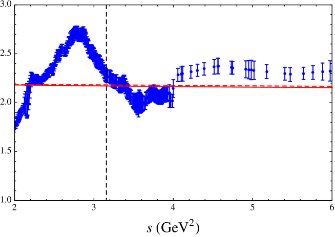
As already mentioned, the aim of this paper is to investigate the validity of the tOPE strategy using data for the EM spectral function obtained from $e^{+}e^{-}\to\mbox{hadrons}(\gamma)$. This is not an exercise of academic interest since, as was shown in Ref. BGMP16 , the assumptions underpinning the tOPE strategy affect the value extracted for $\alpha_{s}$ using this strategy. We will use the recent compilation of exclusive experimental data for the $R$-ratio provided in Ref. KNT18 , which was also recently employed in a determination of $\alpha_{s}$ using a different strategy alphasEM . The sum-of-exclusive-modes part of the compilation of Ref. KNT18 reaches up to $s=4$ GeV², after which the compilation relies on inclusive data sets. We show these data in Fig. 1 in the region $2$ GeV${}^{2}\leq s\leq 6$ GeV², with the transition from exclusive to inclusive regions clearly visible. In Ref. alphasEM it was found that including the much more scarce data above $s=4$ GeV² leads to values of $\alpha_{s}$ consistent with those found from the exclusive data, but without decreasing the error. Also, using Eq. (6) with only values of $s_{0}$ in the inclusive region leads to a still consistent, but higher value of $\alpha_{s}$ with a much larger error. The reason is that the inclusive data for the $R$-ratio tends to be larger than what one would expect from perturbation theory, cf. the red solid and dashed curves in Fig. 1. However, despite the visually apparent tension between the inclusive data and perturbation theory, it was found that the larger values of these data are consistent with it being a statistical fluctuation, given the strong correlations that exist between the inclusive data points at different values of $s$.

Given all this, we will limit ourselves in this paper to an investigation of the tOPE approach using the $R$-ratio data up to $s=4$ GeV²; this is the same region employed in the determination of $\alpha_{s}$ in Ref. alphasEM .

The rest of this paper is organized as follows. Having already reviewed the tOPE strategy and the goal of this paper in this section, we discuss in more detail the assumptions on which our investigation will rely, and elaborate further on our methodology, in Sec. II. Then, in Sec. III, we will present our results, which are shown in Figs. 3 to 10, and explained in the main text. A final section restates our assumptions and contains our conclusions. A preliminary account of this work was presented in Ref. prelim .

II Assumptions and methodology

The tOPE strategy has often been employed previously in analyses of FESRs based on hadronic $\tau$-decay data. As our aim is to use values of $s_{0}$ greater than $m_{\tau}^{2}$ to test the strategy, we will focus instead on FESRs based on EM spectral data. The spectral function obtained from the $R$-ratio is, of course, not the same as the spectral functions obtained from $\tau$ decays. Here, we discuss the differences in some detail, spelling out the assumptions underlying our use of analyses based on the former to cast light on those based on the latter.

It has been advocated, in the literature applying the tOPE strategy to $\tau$-decay data, that analyses of the sum $V+A$ of the non-strange $V$ and $A$ channels are preferable, based on the notion that this sum will be less sensitive to duality violations, and that, in general, non-perturbative effects may be smaller for the sum than for the individual $V$ or $A$ channels. Of course, in the EM case only a $V$-channel spectral function is available, as the photon does not couple to axial currents. There are two reasons to believe that, nevertheless, it is reasonable to expect that useful lessons can be learned by considering the purely $V$-channel EM current only.

First, it was found in Ref. alphasEM that for a determination of $\alpha_{s}$ from $R$-ratio data in the region above about $3.25$ GeV² duality violations can be neglected, with results that are fully consistent with a sum-rule analysis of the $\tau$-based spectral data which modeled duality violations below the $\tau$ mass. This observation implies that the OPE should provide a good representation of the contour integral over $\Pi(s)$ in Eq. (7b) if the radius $s_{0}$ is chosen to be not smaller than approximately $3.25$ GeV². As we will draw our main conclusions from fits of electroproduction data with values of $s_{0}$ above the $\tau$ mass, it therefore appears that the issue of sensitivity to duality violations does not constitute a problem for tests of the tOPE strategy based on EM $V$-channel data.

Moreover, the tOPE-based results obtained in Ref. Pich show excellent consistency for the values of $\alpha_{s}$ extracted from $V$-channel fits and $V+A$-channel fits, employing the weights of Eqs. (10) and (11). The values obtained from $k\ell$ spectral weights differ by slightly more than $1\ \sigma$ between $V$ and $V+A$, while those obtained from optimal weights differ by much less than $1\ \sigma$. In both cases, the quality of the $V$-channel fits is better than that of the $V+A$ channel fits, as measured by the $\chi^{2}$ value per degree of freedom.

Therefore, while we have to assume that $V$-channel-only investigations can shed light on the tOPE strategy as applied to $\tau$ decays, it appears to us that this is, in fact, a rather innocuous assumption.

A second difference between a $\tau$-based analysis and an $R$-ratio-based analysis is that the non-strange spectral functions obtained from $\tau$ decays have isospin $I=1$, while the spectral function obtained from the $R$-ratio has both $I=1$ and $I=0$ components. We thus need to assume that the OPE behavior of the scalar polarization $\Pi_{\rm EM}$ is similar to that of the scalar polarization $\Pi_{I=1}$, if we want to use $R$-ratio based tests to investigate the validity of the tOPE strategy as applied to analyses of hadronic $\tau$-decay data.

In this paper, we will make this assumption, believing that it is well motivated. If the strange-quark mass $m_{s}$ were to be negligibly small, like the up- and down-quark masses, the $I=1$ and $I=0$ currents would be components of an $SU(3)$-flavor multiplet, and any conclusions reached in the study of the EM polarization would directly apply to the $I=1$ case. For $|s|=s_{0}$, the OPE for $\Pi_{\rm EM}(s)$ differs from that for $\Pi_{I=1}(s)$ by terms of order $m_{s}^{2}/s_{0}$, which for $s_{0}\geq m_{\tau}^{2}$ is smaller than $m_{s}^{2}/m_{\tau}^{2}\sim 0.003$. Indeed, in Ref. alphasEM it was found that the effect of $m_{s}$ on the central values of $\alpha_{s}(m_{\tau}^{2})$ and the OPE condensates $C_{6,8,10}$ is significantly smaller than the fit error on the values of these parameters. In addition, we emphasize again that Ref. alphasEM finds excellent agreement between $\alpha_{s}$ determinations based on $R$-ratio and the $\tau$ data, if the OPE is treated consistently and the same strategy is used in both cases alphas1 ; alphas2 ; alphas14 . We conclude that it seems unlikely that the presence of an $I=0$ component in the EM case would have a significant impact on the applicability of the tOPE strategy to $R$-ratio data, in comparison with $\tau$-decay data, at least if the value of $s_{0}$ is large enough.

In our study of the tOPE, we will repeat the $V$-channel fits carried out in Ref. Pich , employing the weights (10) and (11), but now using the $R$-ratio data compilation of Ref. KNT18 . We will consider values of $s_{0}$ ranging from $m_{\tau}^{2}$ to $4$ GeV². If we find a good fit, we will compare the experimental spectral moments $I_{w}^{\rm exp}(s_{0})$ and their theoretical representation based on that fit $I_{w}^{\rm th}(s_{0})$ as follows. First, if we fit at the value $s_{0}=s_{0}^{*}$, we compute the differences

$$\Delta_{w}^{\rm exp}(s_{0};s_{0}^{*}) \equiv I_{w}^{\rm exp}(s_{0})-I_{w}^{\rm exp}(s_{0}^{*})\ ,$$ (12)

$$\Delta_{w}^{\rm th}(s_{0};s_{0}^{*}) \equiv I_{w}^{\rm th}(s_{0})-I_{w}^{\rm th}(s_{0}^{*})\ ,$$

as a function of $s_{0}$. Note that the correlations between spectral integrals at different $s_{0}$, as well as those between OPE integrals at different $s_{0}$, are very strong; working with the differences in Eq. (12) helps to avoid being misled by these correlations when comparing experimental and fitted theory integrals. Then, in order to compare experiment and theoretical representation, we compute the differences

$$\Delta_{w}^{(2)}(s_{0};s_{0}^{*})\equiv\Delta_{w}^{\rm th}(s_{0};s_{0}^{*})-\Delta_{w}^{\rm exp}(s_{0};s_{0}^{*})\ ,$$ (13)

where all correlations, including those between data and fit parameters, are fully taken into account. Considering these double differences avoids any issues with under- or over-estimating errors in the comparison between theory and experiment. Note that, by construction, $\Delta_{w}^{(2)}(s_{0}^{*};s_{0}^{*})=0$, with zero uncertainty.

We will have reason to consider both fully correlated $\chi^{2}$ fits and what we will refer to as “diagonal” fits, where, in the positive quadratic form to be minimized, we only retain the diagonal part of the covariance matrix for the integrated spectral data (in computing this covariance matrix, however, the full data covariance matrix is taken into account). We emphasize that, when computing errors on the fitted parameter values produced by such diagonal fits, we take into account the full covariance matrix for the integrated spectral data, without ignoring any correlations. Although correlated fits are more popular, such diagonal fits can also be a useful tool in cases where the strong correlations make a correlated fit fail. For a detailed explanation of the diagonal fit procedure, we refer the reader to the appendix of Ref. alphas1 . All correlations, including those between data and fit parameters, are always fully taken into account in the computation of the single and double differences $\Delta_{w}^{\rm exp/th}(s_{0};s_{0}^{*})$ and $\Delta_{w}^{(2)}(s_{0};s_{0}^{*})$, for both types of fits.

III Results

$s_{0}^{*}$ (GeV2)	$\chi^{2}/$dof	$p$-value	$\alpha_{s}(m_{\tau}^{2})$	$\alpha_{s}(m_{\tau}^{2})$ (diag)
$m_{\tau}^{2}$	62.7/1	$2\times 10^{-15}$	0.308(4)	0.245(10)
3.6	0.669/1	0.41	0.264(5)	0.256(12)

Table 1: Fit results with optimal weights. We show the fits at $s_{0}^{*}=m_{\tau}^{2}$ and at a value of $s_{0}^{*}$ for which the fit has a $p$-value greater than 10%. Errors shown are fit errors only.

$s_{0}^{*}$ (GeV2)	$\chi^{2}/$dof	$p$-value	$\alpha_{s}(m_{\tau}^{2})$	$\alpha_{s}(m_{\tau}^{2})$ (diag)
$m_{\tau}^{2}$	87.8/1	$7\times 10^{-21}$	0.322(3)	0.281(6)
3.7	1.97/1	0.16	0.277(5)	0.268(9)

Table 2: Fit results with $k\ell$ spectral weights. We show the fits at $s_{0}^{*}=m_{\tau}^{2}$ and at a value of $s_{0}^{*}$ for which the fit has a $p$-value greater than 10%. Errors shown are fit errors only.

We begin with showing and discussing some numerical results from fits employing the tOPE strategy, using fixed-order perturbation theory (FOPT). In Table 1 we show tOPE fit results with optimal weights. We first attempted a correlated fit at $s_{0}^{*}=m_{\tau}^{2}$, precisely following the strategy of Ref. Pich , but employing $R$-ratio data instead of hadronic $\tau$-decay data. We find, as the table shows in the first line, that this fit is very bad. To the right of the double vertical line, we show the corresponding value of $\alpha_{s}(m_{\tau}^{2})$ obtained from a diagonal fit. Not surprisingly, the fit values of $\alpha_{s}(m_{\tau}^{2})$ for these two fits do not agree. We observe that, while the correlated fit produces what, nominally at least, looks like a reasonable result for $\alpha_{s}(m_{\tau}^{2})$, this result cannot be accepted because of the very bad fit quality. The value of $\alpha_{s}(m_{\tau}^{2})$ from the diagonal fit, on the other hand, is very low in comparison with the world average, $\alpha_{s}(m_{\tau}^{2})=0.315(9)$ PDG ; GS17 .

We repeated the same exercise employing $k\ell$ spectral weights, with the results shown in the first line of Table 2. The results look qualitatively similar to those shown in Table 1, but they are not in quantitative agreement.

Clearly, our attempts to apply the tOPE strategy of Ref. Pich at $s_{0}^{*}=m_{\tau}^{2}$ to the electro-production data lead to disastrous results, and an obvious question is what causes this to happen. Assuming that there is no problem with the data (which have been extensively used in Refs. alphasEM ; KNT18 ) leads to the conclusion that the tOPE strategy does not provide a good fit of the $R$-ratio data, while, according to Refs. ALEPH13 ; Pich , it does provide a good fit of the $\tau$-decay data. In fact, it was already observed in Ref. alphasEM that the OPE does not give a good representation of the $w_{\tau}$-spectral integral of the $R$-ratio data for $s_{0}\lesssim 3.25\,\mathrm{GeV}^{2}$ even when no terms from the OPE selected by Eq. (9) were neglected in the analysis. Since consistently good fits were obtained at higher values, $3.25\lesssim s_{0}\leq 4\,\mathrm{GeV}^{2}$, in Ref. alphasEM , it seems reasonable to infer that $s_{0}=m_{\tau}^{2}$ is too small for the OPE to reliably describe the $R$-ratio through the spectral integrals appearing in the FESRs (6) — even more so if, in addition, the OPE is naively truncated. Another possible contributor to the difference might be that the $R$-ratio spectral integrals, being more precise than their counterparts obtained from $\tau$-decay data, provide a more stringent test of the tOPE strategy.

In order to make progress, given this somewhat inconclusive state of affairs, we proceed to consider fits of Eq. (6) using a value $s_{0}=s_{0}^{*}$ larger than $m_{\tau}^{2}$. We increase $s_{0}^{*}$ (in steps of $0.1$ GeV², starting from $s_{0}^{*}=3.2$ GeV²) until the corresponding correlated fit produces a $p$-value greater than 10%. For the optimal and $k\ell$ spectral weight sets, we find this occurs for $s_{0}^{*}=3.6$ GeV² and $s_{0}^{*}=3.7$ GeV², respectively. Both correlated and diagonal fit results are shown in the second lines of Tables 1 and 2, respectively. We see that the results obtained from correlated and diagonal fits are in good agreement for both set of weights. However, the correlated fit values for $\alpha_{s}(m_{\tau}^{2})$ obtained from the optimal and $k\ell$ spectral weight fits are around $2.5~{}\sigma$ or more apart.

Figure 2: $\alpha_{s}(m_{\tau}^{2})$ as a function of $s_{0}$. Blue points (open circles) are correlated optimal-weight fit results, red points (squares) are diagonal optimal-weight fit results, cyan pionts (filled circles) are correlated $k\ell$-spectral weights fit results, and magenta points (triangles) are diagonal $k\ell$-spectral weights fit results. Red, cyan and magenta points are slightly offset horizontally for better visibility.

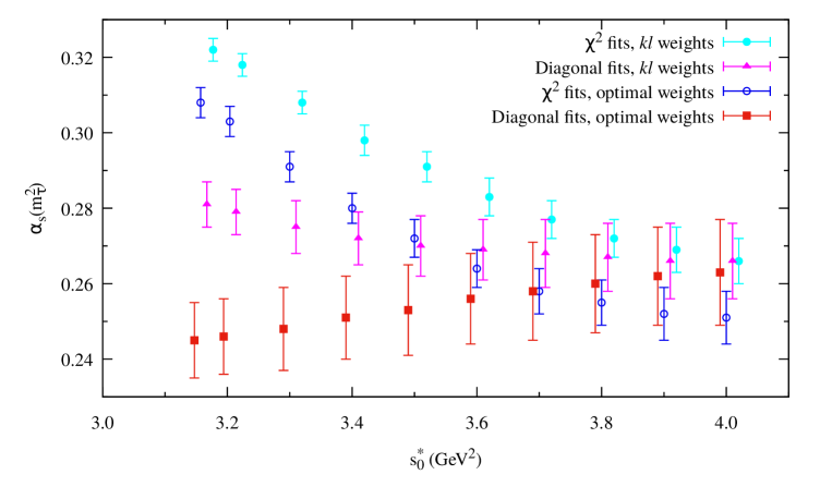
We show results for the strong coupling for each of these types of fits, as a function of $s_{0}^{*}$, in Fig. 2, with correlated fit results for $\alpha_{s}(m_{\tau}^{2})$ for optimal, respectively, $k\ell$ spectral weights shown as blue, respectively, cyan points, and diagonal fit results shown as red, respectively, magenta points. We emphasize that correlated fits with $s_{0}^{*}$ smaller than $3.6$ GeV² have very small $p$-values, which rapidly deteriorate down toward $s_{0}^{*}=m_{\tau}^{2}$. In the region where good correlated fits can be obtained, i.e., for $s_{0}^{*}\,\raisebox{-1.72218pt}{\hbox to0.0pt{$\sim$\hss}}\raisebox{1.72218pt}{$>$}\,3.6$ GeV², there is good agreement with diagonal fits for each set of weights, with the correlated fits yielding the smaller errors. However, there is less good agreement between the results obtained using the optimal and $k\ell$ spectral weight sets. If we were to attempt extracting a value of $\alpha_{s}(m_{\tau}^{2})$ from this collection of fits, we would have to accept a central value of roughly $0.26$–$0.27$, which is again very low compared to the world average; in particular, compared with the values obtained in Refs. alphas1 ; alphasEM ; ALEPH13 ; Pich ; alphas2 ; alphas14 .

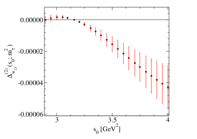
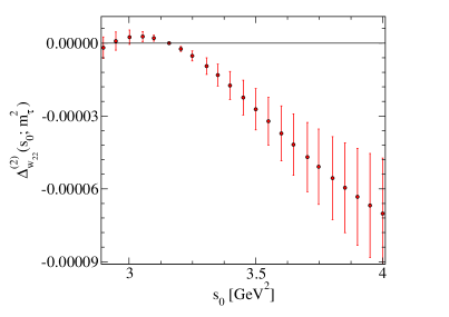
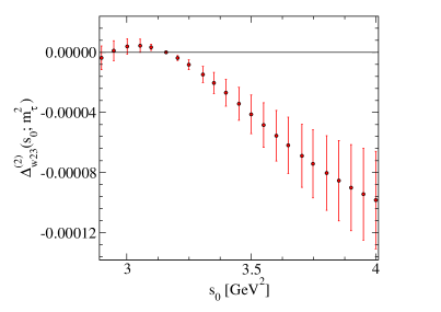
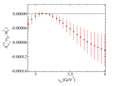
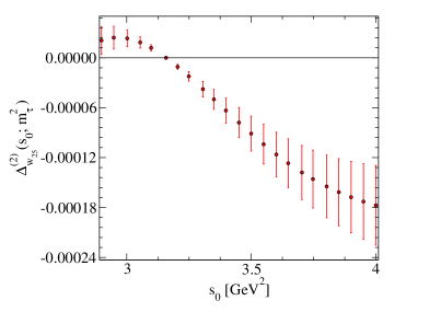
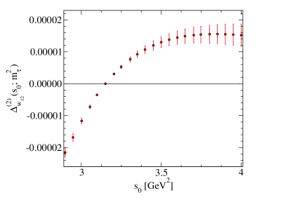
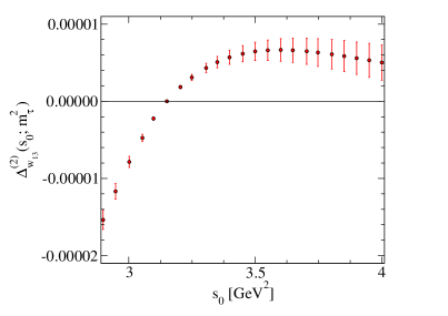
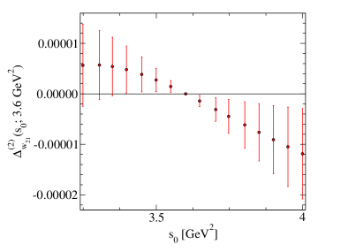
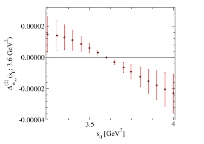
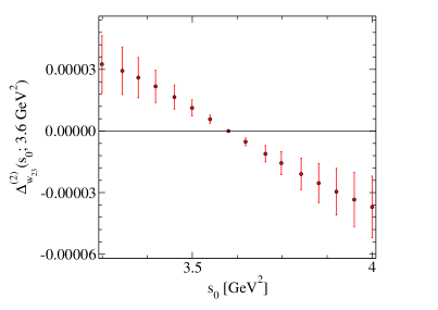
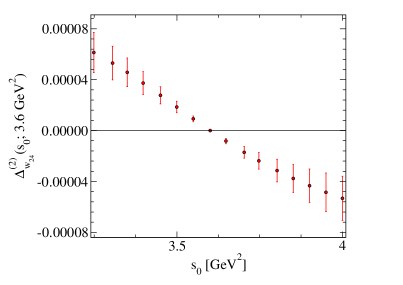
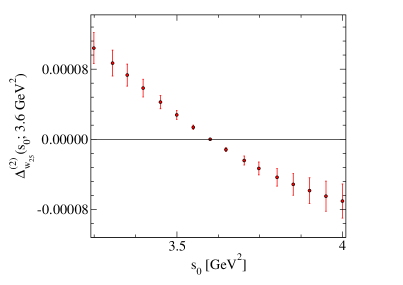
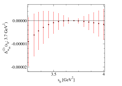
A much more stringent test of the quality of these fits, and thus the assumptions underlying the tOPE strategy, is provided by consideration of the double-differences $\Delta_{w}^{(2)}(s_{0};s_{0}^{*})$ defined in Eq. (13), which we will turn to next. As explained above, a fundamental assumption of the tOPE strategy is that it provides a good theoretical description of the data for the spectral moments $I_{w}^{\rm exp}(s_{0})$ above $s_{0}\approx m_{\tau}^{2}$. Given a fit at some $s_{0}=s_{0}^{*}$, we can vary $s_{0}$, and plot $\Delta_{w}^{(2)}(s_{0};s_{0}^{*})$ as a function of $s_{0}$. If the assumption is correct, we should find good agreement between theory (fitted at $s_{0}^{*}$) and experiment, for any value $s_{0}\geq m_{\tau}^{2}$. This means we should find that $\Delta_{w}^{(2)}(s_{0};s_{0}^{*})=0$ within errors for $m_{\tau}^{2}\leq s_{0}\leq 4$ GeV² for all weights $w$ included in the fit.

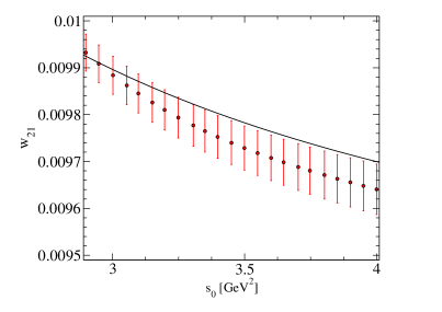
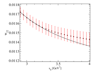
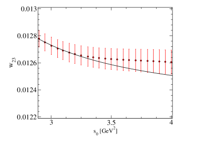
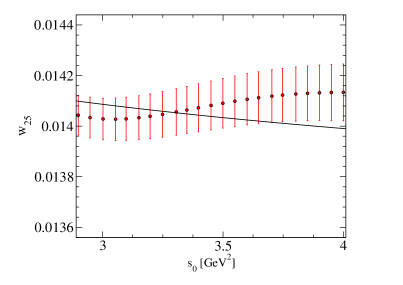
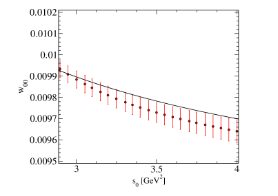
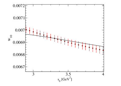
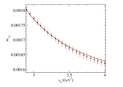
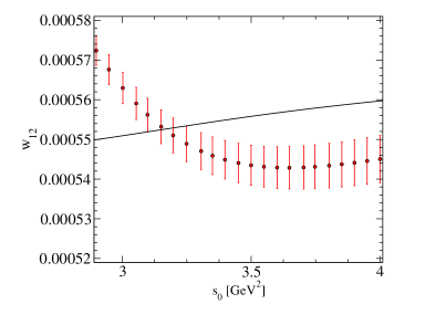
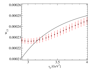
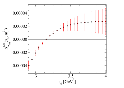
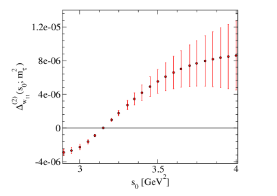
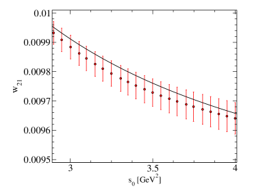
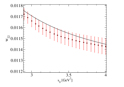
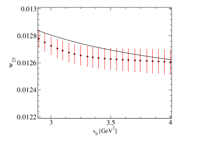
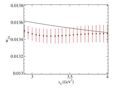
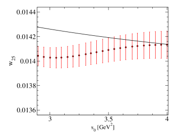
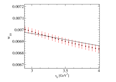
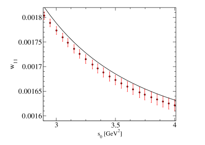
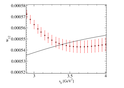
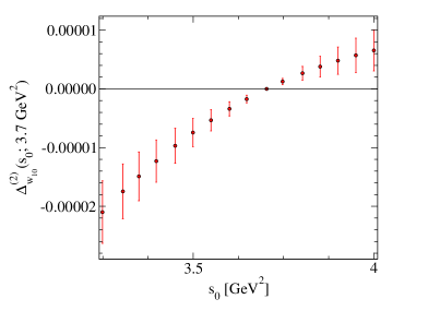
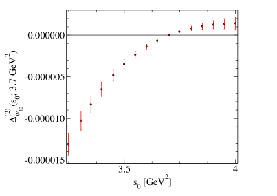
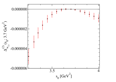
In Figs. 3 to 10 we show the data and the fitted theory curves, as well as the double differences $\Delta_{w}^{(2)}(s_{0};s_{0}^{*})$ for the diagonal fits at $s_{0}^{*}=m_{\tau}^{2}$ in the optimal (Figs. 3 and 4) and $k\ell$ spectral (Figs. 5 and 6) weight cases; for the correlated fit at $s_{0}^{*}=3.6$ GeV² in the optimal weight case (Figs. 7 and 8); and for the correlated fit at $s_{0}^{*}=3.7$ GeV² in the $k\ell$ spectral weight case (Figs. 9 and 10). We emphasize again that all errors shown in all five panels in all four double-difference plots have been computed taking all correlations, including those between data and the fit parameters, into account.

Figures 3, 5, 7, and 9, which show the data compared with the fitted theory curves (using central values for the fit parameters) show what the fits look like, as a function of $s_{0}$. It is clear that the theory, fixed by a fit at $s_{0}=s_{0}^{*}$, does not do a very good job of describing the $s_{0}$ dependence, but, given the strong correlations, it is hard to ascertain, from these figures alone, how bad this problem actually is. It is for this reason that we focus on the comparison between experiment and theory provided by the “double-difference” figures, where we consider the quantity $\Delta_{w}^{(2)}(s_{0};s_{0}^{*})$ as a function of $s_{0}$ for the fixed values of $s_{0}^{*}$ used in the corresponding fits. These results are shown in Figs. 4,  6, 8, and 10.

Three different observations are of relevance to assessing the lessons to be learned from the results shown in the double-difference figures. First, in obtaining results from a fit at $s_{0}=s_{0}^{*}$, it has been assumed that the tOPE strategy provides a valid theory representation at that value of $s_{0}$. This implies, with certainty, that this strategy should provide a good theory representation for any value of $s_{0}\geq s_{0}^{*}$. The plots of $\Delta_{w}^{(2)}(s_{0};s_{0}^{*})$ for $s_{0}>s_{0}^{*}$ directly test this assumption. Second, if the claim is that the tOPE strategy works at $s_{0}=m_{\tau}^{2}$, this implies that, for any $s_{0}^{*}\in[m_{\tau}^{2},4~{}\mbox{GeV}^{2}]$, $\Delta_{w}^{(2)}(s_{0};s_{0}^{*})$ should be consistent with zero for all $s_{0}\geq m_{\tau}^{2}$, irrespective of the value of $s_{0}^{*}$ used in the fit. Finally, for a fit to five spectral moments (whether employing Eq. (10) or Eq. (11)) to be successful, $\Delta_{w}^{(2)}(s_{0};s_{0}^{*})$ has to be consistent with zero as a function of $s_{0}$ for each of the five weights in the set. If $\Delta_{w}^{(2)}(s_{0};s_{0}^{*})$ shows a significant deviation from zero for just one or two weights, this indicates a problem with the fit, and thus with the tOPE strategy.

From Figs. 3, 5, 7, and 9, we see that the fitted theory curves do agree within errors with all five of the corresponding weighted spectral integrals for $s_{0}$ in the vicinity of the tOPE fit point $s_{0}=s_{0}^{*}$. This is, however, not typically the case for $s_{0}$ farther away from $s_{0}^{*}$. One clearly observes, however, that, for many weights, $\Delta_{w}^{(2)}(s_{0};s_{0}^{*})$, shown in Figs. 4, 6,  8, and 10, is not consistent with zero for $m_{\tau}^{2}\leq s_{0}\leq 4$ GeV², and that many points are, in fact, many $\sigma$ away from zero. This is particularly true for the correlated fits shown in Figs. 8 and 10 in the region $3.25$ GeV${}^{2}\leq s_{0}<s_{0}^{*}$. This casts serious doubt on the validity of the tOPE strategy in the whole region we have investigated here, i.e., the region between $s\approx m_{\tau}^{2}$ and $s=4$ GeV².

IV Discussion and conclusion

In this paper, we have continued our investigation of the validity of the truncated OPE (tOPE) approach to FESR analyses, an investigation of relevance, for example, to the determination of $\alpha_{s}$ from such analyses of hadronic $\tau$-decay data. The key observation is that if the tOPE approach works at a “fit point” $s_{0}^{*}$ near $m_{\tau}^{2}$, it should (a) certainly work at higher values of $s_{0}^{*}$, and (b) given a fit at $s_{0}=s_{0}^{*}$ equal to $m_{\tau}^{2}$ or higher, there should be good agreement between the experimental spectral moments and the theory representations employing the OPE parameter fit values at $s_{0}\geq s_{0}^{*}$.

Under rather mild assumptions, tests of these two observations can be carried out using $R$-ratio data, for which very precise results are available up to $s=4$ GeV² KNT18 ; DHMZg . The two assumptions are that (i) it is sufficient to consider only EM vector-channel data (with the axial-channel data available in $\tau$ decays not being accessible through $e^{+}e^{-}\to\mbox{hadrons}$), and (ii) the presence of an $I=0$ component in the $R$-ratio data does not change the behavior of the OPE in an essential way as far as the tOPE strategy is concerned. We discussed these two assumptions, and the reasons for expecting them to be reliable, in detail in Sec. II.

The tOPE approach makes two basic assumptions. The first is that violations of quark-hadron duality can be ignored already at energies as low as the $\tau$ mass, and the second that the expansion in $1/s_{0}$ of the integrated OPE, though in actual fact divergent, acts as if it were rapidly converging already at $s_{0}=m_{\tau}^{2}$. If we assume that in the region $s_{0}\,\raisebox{-1.72218pt}{\hbox to0.0pt{$\sim$\hss}}\raisebox{1.72218pt}{$>$}\,m_{\tau}^{2}$ duality violations are relatively unimportant (an assumption that is consistent with the results of Ref. alphasEM ), the question centers on the nature of the OPE for values of $Q^{2}$ with $|Q^{2}|=s_{0}$ in this region.

Our central results are shown in Figs. 4, 6, 8, and 10. If the tOPE were to be valid, they should show data points consistent with zero for all $s_{0}\geq m_{\tau}^{2}$. Instead, these figures show very significant disagreements, as a function of $s_{0}$, between the experimental values of the spectral moments and the theory representations based on the tOPE fits at various fit points $s_{0}^{*}$, for both the optimal-weight- and $k\ell$-spectral-weight-based fits. We emphasize that the error bars shown for the double differences, defined in Eq. (13), take all correlations into account, including those between data and the fit parameter values.

The first two of these figures show the results of diagonal fits at $s_{0}^{*}=m_{\tau}^{2}$, which we considered after we found that correlated fits do not work at this $s_{0}^{*}$ (cf. Tables 1 and 2). More important are the fits at $s_{0}^{*}=3.6$ GeV² (for optimal weights, shown in Fig. 8) and $s_{0}^{*}=3.7$ GeV² (for $k\ell$ spectral weights, shown in Fig. 10). These are correlated $\chi^{2}$ fits with acceptable $p$-values, where the figures nonetheless show very serious mismatches between the experimental data and the theory representations provided by the fits. We observe that if the tOPE strategy does not work for a value of $s_{0}^{*}$ significantly larger than $m_{\tau}^{2}$, it certainly cannot be expected to be reliable at $s_{0}^{*}=m_{\tau}^{2}$, thus making our tests at $s_{0}^{*}=m_{\tau}^{2}$ less relevant. Nevertheless, the fact that correlated fits at $s_{0}^{*}=m_{\tau}^{2}$ do not work stands in sharp contrast to what is found with data from hadronic $\tau$ decays BGMP16 ; Pich .

We may also ask what our results imply for the OPE itself, rather than just for the tOPE strategy. Our tests probe the integrated OPE up to dimension 16, for both the optimal and $k\ell$ spectral weight sets. As the OPE is (at best) an asymptotic expansion, the question is to which order one can expect to be able to use it while still having the truncated expansion approach the underlying true physical value. The answer to this question will, of course, depend on the value of $s_{0}$. The analysis in Ref. alphasEM showed that the OPE provides a consistent representation of the EM vacuum polarization up to dimension $D=10$, a conclusion supported, in particular, by the consistency of the results for the effective $D=6$ condensate, $C_{6}$, obtained using different weights with degree up to $4$, in the region $m_{\tau}^{2}\leq s_{0}\leq 4\,\mathrm{GeV}^{2}$. It is possible that the OPE starts to already diverge before one reaches the term of dimension $16$ for $s_{0}$ in the range between $m_{\tau}^{2}$ and 4 GeV², but it is also possible that it approaches the (unknown) exact answer reasonably well, to this order, and in this range. Our tests leave this question undecided. What they do show is that even if the OPE is still approaching the true answer out to $D=16$, it is not doing so rapidly enough that terms with $D>10$ (for the optimal weights) or $D>8$ (for the $k\ell$ spectral weights) can be neglected, in the sum rules considered here. In any case, our analysis provides a clear message that it is safest to restrict the analysis to those observables which only receive a contribution from the lower-dimension terms in the OPE.

Our main conclusion is that even if one considers an energy region in which duality violations are likely to be strongly suppressed, the tOPE strategy leads to inconsistent results, thus invalidating the neglect of higher-order terms in the OPE in that energy region. Taken together with our earlier investigations of the tOPE strategy reported in Ref. BGMP16 , the implication is that the tOPE strategy is not a reliable one. It should thus no longer be employed, for example, in the extraction of $\alpha_{s}$ from hadronic $\tau$ decays or $R$-ratio data, up to at least $s=4$ GeV², particularly since an alternative method which does not suffer from the shortcomings of the tOPE strategy exists alphas1 ; alphasEM ; alphas2 ; alphas14 .

Acknowledgments

DB, KM and SP would like to thank the Department of Physics and Astronomy at San Francisco State University for hospitality, and MG would like to thank the Department of Mathematics and Statistics at York University for hospitality. The work of DB is supported by the São Paulo Research Foundation (FAPESP) Grant No. 2015/20689-9 and by CNPq Grant No. 309847/2018-4. The work of MG is supported by the U.S. Department of Energy, Office of Science, Office of High Energy Physics, under Award Number DE-FG03-92ER40711. KM is supported by a grant from the Natural Sciences and Engineering Research Council of Canada. SP is supported by CICYTFEDER-FPA2017-86989-P and by Grant No. 2017 SGR 1069.

Figure 3: Comparison of $I_{w}^{\rm exp}(s_{0})$ with $I_{w}^{\rm th}(s_{0})$ with parameter values obtained from diagonal fits with optimal weights, as a function of $s_{0}$ with $s_{0}^{*}=m_{\tau}^{2}$.

Figure 4: The double differences, $\Delta^{(2)}_{w}(s_{0};s_{0}^{*})$, obtained from diagonal fits with optimal weights, as a function of $s_{0}$ with $s_{0}^{*}=m_{\tau}^{2}$.

Figure 5: Comparison of $I_{w}^{\rm exp}(s_{0})$ with $I_{w}^{\rm th}(s_{0})$ with parameter values obtained from diagonal fits with $k\ell$ spectral weights, as a function of $s_{0}$ with $s_{0}^{*}=m_{\tau}^{2}$.

Figure 6: The double differences, $\Delta^{(2)}_{w}(s_{0};s_{0}^{*})$, obtained from diagonal fits with $k\ell$ spectral weights, as a function of $s_{0}$ with $s_{0}^{*}=m_{\tau}^{2}$.

Figure 7: Comparison of $I_{w}^{\rm exp}(s_{0})$ with $I_{w}^{\rm th}(s_{0})$ with parameter values obtained from correlated fits with optimal weights, as a function of $s_{0}$ with $s_{0}^{*}=3.6$ GeV².

Figure 8: The double differences, $\Delta^{(2)}_{w}(s_{0};s_{0}^{*})$, obtained from correlated fits with optimal weights, as a function of $s_{0}$ with $s_{0}^{*}=3.6$ GeV².

Figure 9: Comparison of $I_{w}^{\rm exp}(s_{0})$ with $I_{w}^{\rm th}(s_{0})$ with parameter values obtained from correlated fits with $k\ell$ spectral weights, as a function of $s_{0}$ with $s_{0}^{*}=3.7$ GeV².

Figure 10: The double differences, $\Delta^{(2)}_{w}(s_{0};s_{0}^{*})$, obtained from correlated fits with $k\ell$ spectral weights, as a function of $s_{0}$ with $s_{0}^{*}=3.7$ GeV².

References

- (1)
- (2) Y. S. Tsai, Phys. Rev. D 4, 2821 (1971) Erratum: [Phys. Rev. D 13, 771 (1976)].
- (3) J. Erler, Rev. Mex. Fis. 50, 200 (2004) [hep-ph/0211345].
- (4) R. Shankar, Phys. Rev. D 15, 755 (1977); R. G. Moorhouse, M. R. Pennington and G. G. Ross, Nucl. Phys. B 124, 285 (1977); K. G. Chetyrkin and N. V. Krasnikov, Nucl. Phys. B 119, 174 (1977); K. G. Chetyrkin, N. V. Krasnikov and A. N. Tavkhelidze, Phys. Lett. B 76, 83 (1978); N. V. Krasnikov, A. A. Pivovarov and N. N. Tavkhelidze, Z. Phys. C 19, 301 (1983); E. G. Floratos, S. Narison and E. de Rafael, Nucl. Phys. B 155, 115 (1979); R. A. Bertlmann, G. Launer and E. de Rafael, Nucl. Phys. B 250, 61 (1985).
- (5) E. Gamiz et al., JHEP, 0301, 060 (2003); Phys. Rev. Lett., 94, 011803 (2005); PoS, KAON 2007, 008 (2008).
- (6) K. Maltman, et al., Nucl. Phys. Proc. Suppl., 189, 175 (2009); K. Maltman, Nucl. Phys. Proc. Suppl., 218, 146 (2011).
- (7) R. J. Hudspith, R. Lewis, K. Maltman and J. Zanotti, Phys. Lett. B 781, 206 (2018) [arXiv:1702.01767 [hep-ph]].
- (8) M. Davier, L. Girlanda, A. Höcker and J. Stern, Phys. Rev. D 58, 096014 (1998) [hep-ph/9802447]; S. Dürr and J. Kambor, Phys. Rev. D 61, 114025 (2000) [hep-ph/9907539]; M. Golterman, K. Maltman and S. Peris, Phys. Rev. D 89, no. 5, 054036 (2014) [arXiv:1402.1043 [hep-ph]].
- (9) E. C. Poggio, H. R. Quinn and S. Weinberg, Phys. Rev. D 13, 1958 (1976).
- (10) K. Maltman, Phys. Lett. B 440, 367 (1998); C. A. Dominguez and K. Schilcher, Phys. Lett. B bf 448, 93 (1999).
- (11) O. Catà, M. Golterman and S. Peris, Phys. Rev. D 79, 053002 (2009) [arXiv:0812.2285 [hep-ph]].
- (12) D. Boito, O. Catà, M. Golterman, M. Jamin, K. Maltman, J. Osborne and S. Peris, Phys. Rev. D 84, 113006 (2011) [arXiv:1110.1127 [hep-ph]].
- (13) D. Boito, I. Caprini, M. Golterman, K. Maltman and S. Peris, Phys. Rev. D 97, 054007 (2018) [arXiv:1711.10316 [hep-ph]].
- (14) D. Boito, M. Golterman, K. Maltman and S. Peris, Phys. Rev. D 95, 034024 (2017) [arXiv:1611.03457 [hep-ph]].
- (15) D. Boito, M. Golterman, A. Keshavarzi, K. Maltman, D. Nomura, S. Peris and T. Teubner, Phys. Rev. D 98, no. 7, 074030 (2018) [arXiv:1805.08176 [hep-ph]].
- (16) F. Le Diberder and A. Pich, Phys. Lett. B 289, 165 (1992).
- (17) M. Davier, A. Höcker, B. Malaescu, C. Z. Yuan and Z. Zhang, Eur. Phys. J. C 74, 2803 (2014) [arXiv:1312.1501 [hep-ex]].
- (18) A. Pich and A. Rodríguez-Sánchez, Phys. Rev. D 94, 034027 (2016) [arXiv:1605.06830 [hep-ph]].
- (19) A. Keshavarzi, D. Nomura and T. Teubner, Phys. Rev. D 97, no. 11, 114025 (2018) [arXiv:1802.02995 [hep-ph]].
- (20) D. Boito, M. Golterman, K. Maltman and S. Peris, SciPost Phys. Proc. 1, 053 (2019) [arXiv:1811.01581 [hep-ph]].
- (21) D. Boito, M. Golterman, M. Jamin, A. Mahdavi, K. Maltman, J. Osborne and S. Peris, Phys. Rev. D 85, 093015 (2012) [arXiv:1203.3146 [hep-ph]].
- (22) D. Boito, M. Golterman, K. Maltman, J. Osborne and S. Peris, Phys. Rev. D 91, 034003 (2015) [arXiv:1410.3528 [hep-ph]].
- (23) A. A. Pivovarov, Z. Phys. C 53, 461 (1992) [Sov. J. Nucl. Phys. 54, 676 (1991)] [Yad. Fiz. 54 (1991) 1114] [arXiv:hep-ph/0302003]; F. Le Diberder and A. Pich, Phys. Lett. B 286, 147 (1992).
- (24) M. Beneke and M. Jamin, JHEP 0809, 044 (2008) [arXiv:0806.3156 [hep-ph]].
- (25) M. Beneke, D. Boito and M. Jamin, JHEP 1301, 125 (2013) [arXiv:1210.8038 [hep-ph]].
- (26) M. Tanabashi et al. [Particle Data Group], Phys. Rev. D 98, no. 3, 030001 (2018).
- (27) G. P. Salam, arXiv:1712.05165 [hep-ph].
- (28) M. Davier, A. Höcker, B. Malaescu and Z. Zhang, Eur. Phys. J. C 77, no. 12, 827 (2017) [arXiv:1706.09436 [hep-ph]].