Hybridized Threshold Clustering for Massive Data

Abstract

As the size $n$ of datasets become massive, many commonly-used clustering algorithms (for example, $k$-means or hierarchical agglomerative clustering (HAC) require prohibitive computational cost and memory. In this paper, we propose a solution to these clustering problems by extending threshold clustering (TC) to problems of instance selection. TC is a recently developed clustering algorithm designed to partition data into many small clusters in linearithmic time (on average). Our proposed clustering method is as follows. First, TC is performed and clusters are reduced into single “prototype” points. Then, TC is applied repeatedly on these prototype points until sufficient data reduction has been obtained. Finally, a more sophisticated clustering algorithm is applied to the reduced prototype points, thereby obtaining a clustering on all $n$ data points. This entire procedure for clustering is called iterative hybridized threshold clustering (IHTC). Through simulation results and by applying our methodology on several real datasets, we show that IHTC combined with $k$-means or HAC substantially reduces the run time and memory usage of the original clustering algorithms while still preserving their performance. Additionally, IHTC helps prevent singular data points from being overfit by clustering algorithms.

Keywords: Threshold Clustering, Hybridized Clustering, Instance Selection, Prototypes, Massive Data

1 Introduction

Clustering, also known as unsupervised learning, is a well-studied problem in machine learning. It aims to group units with similar features together and separate units with dissimilar features (Friedman et al., 2001). Cluster analysis has been used in many fields like biology, management, pattern recognition, etc. Additionally, many methods (for example, $k$-means clustering, hierarchical agglomerative clustering, etc.) have been developed that successfully tackle the clustering problem.

However, enormous amounts of data are collected every day. For example, Walmart performs more than 1 million customer transactions per hour (Cukier, 2010), and Google performs more than 3 billion searches per day (Sullivan, 2015). This becomes a massive accumulation of data. When working with data of such a large size, many of the state-of-the-art clustering methods become intractable. That is, massive data requires novel statistical methods to process this data; research on scaling up existing statistical algorithms and scaling down the size of data without loss of information is of critical importance (Jordan and Mitchell, 2015).

Instance selection is a commonly-used pre-possessing method for scaling down the size of data (Liu and Motoda, 1998; Blum and Langley, 1997; Liu and Motoda, 2002). The goal of instance selection is to shorten the execution time of data analysis by reducing data size $n$ while maintaining the integrity of data (Olvera-López et al., 2010). Instance selection methods rely on sampling, classification algorithms, or clustering algorithms. Previous work has shown methods reliant on clustering have better performance (accuracy) than some methods that rely on classification (Riquelme et al., 2003; Raicharoen and Lursinsap, 2005; Olvera-López et al., 2007, 2008, 2010). However, current instance selection methods that rely on classification often have faster runtimes.

On the other hand, threshold clustering (TC) is a recently developed method for clustering that is extremely efficient. TC is a method of clustering units so that each cluster contains at least a pre-specified number of units $t^{*}$ while ensuring that the within-cluster dissimilarities are small. Previous work has shown that, when the objective is to minimize the maximum within-cluster dissimilarities, a solution within a factor of four of optimal can often be obtained in $O(t^{*}n)$ time and space when the $(t^{*}-1)$-nearest-neighbors graph is given (Higgins et al., 2016). The runtime and memory usage required for TC is smaller compared to other clustering methods, for example, $k$-means and hierarchical agglomerative clustering (HAC).

In this paper, we propose the use of TC for instance selection. The proposed method, which is called iterated threshold instance selection (ITIS), works as follows. For a given $t^{*}$, TC is applied on $n$ units to form $n^{*}$ clusters; each cluster will contain at least $t^{*}$ units. Then prototypes are formed by finding the center of each cluster. TC is applied again to the $n^{*}$ prototypes if the data is not sufficiently reduced. Otherwise, the procedure is stopped.

We also propose using ITIS as a pre-processing step on large data to allow for the use of more sophisticated clustering methods. First, ITIS is applied to form a sufficiently small set of prototypes. Then, a more sophisticated clustering algorithm (for example $k$-means, HAC) is applied on this set of prototypes. Finally, a clustering on all $n$ units is obtained by ”backing out” the cluster assignments for the prototypes—for each prototype, the units used to form the prototype are determined; these units are assigned to the same cluster assigned to the prototype. This clustering process on all $n$ units is called Iterative Hybridized Threshold Clustering (IHTC).

We show, using simulations and applications of our algorithm to six large datasets, that IHTC combined with other clustering algorithms reduces the run time and memory usage of the original clustering algorithms while still preserving their performance. Additionally, we show IHTC also prevents singular data points from being overfit by desired clustering methods. Specifically, for $m$ iterations of ITIS at size threshold $t^{*}$, IHTC ensures that each cluster contains at least $(t^{*})^{m}$ units.

The rest of this paper is organized as follows. A brief summary about clustering algorithms ($k$-means, HAC, TC) is given in section 2. Section 3 shows how to extend threshold clustering as an instance selection method and combine the iterated threshold instance selection method with other clustering methods. A simulation study is presented in section 4 and application of our methods on real datasets are presented in section 5. The last section discuss about our method.

2 Notation and Preliminaries

Consider a dataset with n units, numbered 1 through $n$. Each unit $i$ has a response vector $\mathbf{y}_{i}$ and a $d$-dimensional covariate vector $\mathbf{x}_{i}=(x_{i1},x_{i2},\ldots,x_{id})$. For each pair of units $i,j$, the dissimilarity between $i$ and $j$, denoted $d_{ij}$, can be computed. Often, the dissimilarity is chosen so that, if units $i$ and $j$ have similar values of covariates $\mathbf{x}$, then $d_{ij}$ is small. We assume that $d_{ij}\geq 0$, and that dissimilarities satisfy the triangle inequality; for any units $i$, $j$, $\ell$,

$$d_{ij}+d_{jk}\geq d_{i\ell}$$ (1)

Common choices of dissimilarities include Euclidean distance, Manhattan distance and average distance.

We define a clustering of a set of units as a partitioning of units such that units within each cluster of a partition have “small dissimilarity” and units belonging to two different clusters have “large dissimilarity.” That is, at minimum, a clustering $\mathbf{v}=\{V_{1},V_{2},\ldots,V_{m}\}$ will satisfy the following properties:

1. (Non-empty): $V_{\ell}\neq\emptyset$ for all $V_{\ell}\in\mathbf{v}$.

2. (Spanning): For all units $i$, there exists a cluster $V_{\ell}\in\mathbf{v}$ such that $i\in V_{\ell}$.

3. (Disjoint): For any two clusters $V_{\ell},V_{\ell^{\prime}}\in\mathbf{v}$, $V_{\ell}\cap V_{\ell^{\prime}}=\emptyset$

The way of measuring “large” and “small” cluster dissimilarity will vary across clustering algorithms.

There are currently hundreds of available methods for clustering units. Moreover, some of these methods may be combined to construct additional hybridized clustering methods—our procedure for hybridizing is the major contribution of this paper. For brevity, we apply our hybridizing procedure to two clustering methods—$k$-means and hierarchical clustering—with a note that this procedure may be applied to many other types of clustering. We now give a brief summary of these clustering methods.

2.1 K-means Clustering

The $k$-means clustering algorithm (Lloyd, 1982) is one of the most widely used and effective methods that attempts to partition units into exactly $k$-clusters.

The $k$-means clustering algorithm proceeds as follows:

1. (Initialization) Randomly select a set of $k$ units (referred as centers) from the dataset. $K$ denote the number of clusters and it should be pre-specified.

2. (Assignment) Assign all the units to the nearest center, based on squared Euclidean distance, to form $k$ temporary clusters.

3. (Updating) Recompute the mean of each cluster. Replace the centers with the new $k$ cluster means.

4. (Terminate) Repeat step 2 and  3 until there is no further change for the centers.

The time complexity for the $k$-means clustering algorithm is $O(nkLd)$ and the space complexity is $O((k+n)d)$ (Hartigan and Wong, 1979; Firdaus and Uddin, 2015) where $d$ is the number of attributes for each unit, $L$ is the number of iterations taken by the algorithm to converge.

The $k$-means algorithm suffers from a number of drawbacks  (Hastie et al., 2009). First, there tends to be high sensitivity to the selection of initial units in Step 1. Additionally, it tends to overfit isolated units leading to some clusters containing only a few units. Finally, the number of clusters $k$ is fixed; if $k$ is misspecified, $k$-means may perform poorly. In particular, many methods have been developed to mitigate problems due to initialization (Fränti et al., 1997; Frnti et al., 1998; Arthur and Vassilvitskii, 2007; Fränti and Kivijärvi, 2000).

2.2 Hierarchical Agglomerative Clustering

Hierarchical agglomerative clustering (HAC) (Ward Jr, 1963) is a ”bottom up” approach that aims to build a hierarchy clusters. It initially treats each unit as a cluster and then continues to merge two clusters together until only one cluster remains. HAC does not require a pre-specified number of clusters; the desired number of clusters can be obtained by using a dendogram—a tree that shows how the units are merged.

The HAC proceeds as follows:

1. (Initial Clusters) Start with $n$ clusters, each cluster only contains one unit.

2. (Merge) Merge the closest (most similar) pair of clusters into a single cluster.

3. (Updating) Recompute the distance between the new cluster and the original clusters.

4. (Terminate) Repeat step 2 and  3 until one cluster remains, the cluster contains $n$ units.

HAC requires linkage criteria to measure inter-cluster distance, but initialization and the choice of $k$ is no longer a problem. However, the time complexity of HAC is $O(n^{2}\log(n))$ (Kurita, 1991) and space complexity is $O(n^{2})$ (Jain et al., 1999). This complexity limits its application to massive data. Another hindrance of HAC is that every merging decision is final. Once two clusters are merged into a new cluster, there is no way to partition the new cluster in later steps.

2.3 Threshold Clustering (TC)

Our hybridization method makes use of a recently developed clustering method called threshold clustering (TC). Initially this method was developed for performing statistical blocking of massive experiments (Higgins et al., 2016). TC differs in two significant ways from traditional clustering approaches. First, TC does not fix the number of clusters formed, but instead, it ensures that each cluster contains a pre-specified number of units. Thus, TC is an effective way of obtaining many clusters, with each containing only a few units. Second, TC ensures the formation of a clustering with a small maximum within-group dissimilarity—more precisely, TC finds approximately optimal clustering with respect to a bottleneck objective—as opposed to an average or median within-group dissimilarity. The bottleneck objective is chosen not only to prevent largely dissimilar units from being grouped together, but also because these types of optimization problems often have approximate solutions that can be found efficiently (Hochbaum and Shmoys, 1986).

More precisely, let $\mathbf{B}(t^{*})$ denote the set of all threshold clusterings—those clusterings $\mathbf{v}$ such that $|V_{\ell}|\geq t^{*}$ for each cluster $V_{\ell}\in\mathbf{v}$. The bottleneck threshold partitioning problem (BTPP) is to find the threshold clustering that minimizes the maximum within-cluster dissimilarity. That is, BTPP aims to find $\mathbf{v}^{\dagger}\in\mathbf{B}(t^{*})$ satisfying:

$$\max_{V_{\ell}\in\mathbf{v}^{\dagger}}\max_{ij\in V_{\ell}}d_{ij}=\min_{\mathbf{v}\in\mathbf{B}(t^{*})}\max_{V_{\ell}\in\mathbf{v}}\max_{ij\in V_{\ell}}d_{ij}\equiv\lambda;$$ (2)

here, $\lambda$ is the optimal value of the maximum within-cluster dissimilarity.

It can be shown that BTPP is NP-hard, and in fact, no $(2-\epsilon)$–approximation algorithm for BTPP exists unless $\text{P}=\text{NP}$. However, Higgins et al. (2016) develop a threshold clustering algorithm (for clarity, the abbreviation TC refers specifically to this algorithm) to find a threshold clustering with maximum within-cluster dissimilarity at most $4\lambda$. That is, TC is a 4–approximation algorithm for BTPP. The time and space requirement for TC are $O(t^{*}n)$ outside of the construction of a $t^{*}$–nearest neighbors graph (Higgins et al., 2016). Constructing a nearest neighbor graph is a well-studied problem for which many efficient algorithms already exist. At worst, forming a $k$–nearest neighbor graph requires $O(n^{2}\log n)$ time (Knuth, 1998); however, if the covariate space is low-dimensional, this construction may only require $O(kn\log n)$ time (Friedman et al., 1976; Vaidya, 1989). Hence, TC may be used for large datasets, especially when the threshold $t^{*}$ and the dimensionality of the covariate space are small.

TC uses graph theoretic ideas in its implementation. See Appendix C for graph theory definitions. TC with respect to a pre-specified minimum cluster size threshold $t^{*}$ is performed as follows:

1. (Construct nearest-neighbor subgraph) Construct a $(t^{*}-1)$-nearest-neighbors subgraph $NG_{t^{*}-1}$ with respect to the dissimilarity measure $d_{ij}$ (We use Euclidean distance to measure dissimilarity in this paper).

2. (Choose set of seeds) Choose a set of units $\mathbf{S}$ such that

   1. For any two distinct units $i,j\in\mathbf{S}$, there is no walk of length one or two in $NG_{t^{*}-1}$ from $i$ to $j$.

   2. For any unit $i\notin\mathbf{S}$, there is a unit $j\in\mathbf{S}$ such that there exists a walk from $i$ to $j$ of length at most two in $NG_{t^{*}-1}$.

   Units in $S$ are known as seeds.

3. (Grow from seeds) For each $\ell\in\mathbf{S}$, form a cluster of units $V^{*}_{\ell}$ comprised of unit $\ell$ and all units adjacent to $\ell$ in $NG_{t^{*}-1}$.

4. (Assign remaining vertices) Some units $j$ may not be assigned to a cluster yet. These units are a walk of length two from at least one seed $\ell\in\mathbf{S}$ in $NG_{t^{*}-1}$. Assign the unassigned units to the cluster associated with seed $\ell$. If there are several choices of seeds, choose the one that with the smallest dissimilarity $d_{\ell j}$.

The set of clusters $\mathbf{v}=\{V^{*}_{\ell}\}_{\ell\in\mathbf{S}}$ form a threshold clustering. Additionally, polynomial-time improvements to this algorithm—for example, in selecting cluster seeds or splitting large clusters—may improve the performance of TC without substantially increasing its runtime. An implementation of TC can be found in the R package scclust (Savje et al., 2017).

3 Extension of Threshold Clustering

We now describe two extensions of TC: applying TC to instance selection problems and using TC as a preprocessing step for statistical clustering methods.

3.1 Threshold clustering as instance selection

Instance selection methods are used in massive data settings to efficiently scale down the size of the data (Leyva et al., 2015). Common techniques for instance selection include subsampling (Pooja, 2013) and constructing prototypes (Plasencia-Calaña et al., 2014)—pseudo data points where each prototype represents a group of similar individual units. These methods tend to work quite well for massive data applications.

Suppose the researcher desires to reduce the size of the data by a factor of $\alpha$. We propose the following method for instance selection, which we call iterated threshold instance selection (ITIS):

1. (Threshold clustering) Perform threshold clustering with respect to a small size threshold $t^{*}$ (for example, $t^{*}=2$) on the $n$ data points to form $n^{*}$ clusters, each containing $t^{*}$ or more points.

2. (Create prototypes) Compute a center point for each of the $n^{*}$ groups (for example, centroid or medoid).

3. (Terminate or continue) If the data is reduced by a factor of $\alpha$, stop. Otherwise, replace the $n$ data points with the $n^{*}$ centers and go back to Step 1.

An illustration of the ITIS procedure is given in Figure 1.

Figure 1: An illustration of iterated threshold instance selection (ITIS) with threshod $t^{*}=2$ on a sample of $n=30$ data points drawn from a bivariate Gaussian mixture model. In (2.a), each unit is represented by a point. Applying threshold clustering on the data, 12 clusters are formed in (2.b). A prototype is formed for each of the 12 groups in (2.c). In (2.d), apply threshold clustering on the prototype, 5 clusters are formed. 5 prototypes are formed for the 5 clusters, the results are shown in (2.e). For this illustration, We perform two iterations of ITIS.

Ultimately, the choice of the number of iterations of ITIS $m$ depends on the researcher. For example, a researcher may want to scale down the data as little as necessary in order to perform a computationally intensive statistical procedure on the reduced data. Additionally, the performance of TC may depend on the dissimilarity measure $d_{ij}$; in our experience, using the standardized Euclidean distance tends to work well.

The running time of $m$ iterations of ITIS is $O(t^{*}mn\log n)$. Moreover, since the size of the data is reduced by a factor of $t^{*}$ with each iteration, the computational bottleneck of ITIS becomes the construction of a $t^{*}$–nearest-neighbors graph on all $n$ units. This also suggests that the computation required of ITIS may be drastically improved through the discovery of methods for parallelization of threshold clustering.

The iterative nature of ITIS does have a drawback; with each iteration, the prototype units become less similar to the units comprising the prototype. In particular, the approximate optimality property of TC may not hold if $m>1$. However, simulations suggest that this issue is not severe in massive data settings. Alternatively, approximate optimality may be preserved by choosing $t^{*}=\alpha$ and running one iteration of ITIS. However, the one iteration version does not seem to be as promising under massive data settings since the runtime of TC increases as $t^{*}$ increases. See Appendix A for details.

3.2 Iterative Hybridized Threshold Clustering

Often, researchers would like to use certain clustering methods (for example, $k$-means, HAC, etc.) because of favorable or familiar properties of these clustering methods. However, under massive data settings, using such clustering techniques may not be feasible because of prohibitive computational costs. We propose the following method for using ITIS as a pre-processing step on all $n$ units to allow for the use of more sophisticated clustering methods. We call this procedure Iterative Hybridized Threshold Clustering (IHTC). It works as follows:

1. (Create prototypes) Perform iterative threshold instance selection with respect to a size threshold $t^{*}$ on the $n$ data points $m$ times to form prototypes.

2. (Cluster prototypes) Cluster the prototypes (for example, using $k$-means) obtained by 1.

3. (”Back out” assignment) For each prototype, determine which of the original $n$ units contributed to the formation of that prototype and assign these units to the cluster belonging to the prototype.

Figure 2 gives an illustration of IHTC with $k$-means.

Figure 2: An illustration of hybridized threshold clustering with $k$-means on bivariate data: $n=20,k=3,t^{*}=2$. In graph (3.a), each unit is represented by a point. Applying threshold clustering on the data, 7 clusters are formed in (3.b). A prototype is formed for each of the 7 groups in (3.c). In (3.d), $k$-means clustering is performed on the prototypes. The ”backed out” final clustering results are given in (3.e).

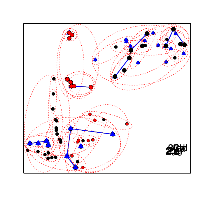
IHTC reduces the size of the data by a factor of $(t^{*})^{m}$, which can improve the efficiency of the original clustering algorithm. Additionally, IHTC also prevents overfitting of individual points, which may lead to a more effective clustering regardless with just a couple iterations of IHTC. Specifically, for $m$ iterations of ITIS at size threshold $t^{*}$, IHTC ensures that each cluster contains at least $(t^{*})^{m}$ units. Finally, we note that IHTC may be applied to most other clustering algorithms—not just $k$-means or HAC.

4 Simulation

We first demonstrate properties of IHTC using simulated data. We apply IHTC to samples of varying sizes where each data point is sampled from a mixture of three bivariate Gaussian distributions. Specifically, samples are drawn independently from a distribution with pdf:

$$f(\mathbf{x})=0.5p(\mathbf{x}|\mathbf{\mu_{1},\Sigma_{1}})+0.3p(\mathbf{x}|\mathbf{\mu_{2},\Sigma_{2}})+0.2p(\mathbf{x}|\mathbf{\mu_{3},\Sigma_{3}})$$

where $p(\mathbf{x}|\mathbf{\mu_{j},\Sigma_{j}})$ is the pdf of a Gaussian with parameters $\mathbf{\mu_{j}}$ and $\mathbf{\Sigma_{j}}$, $j=1,2,3$,

$$\mathbf{\mu_{1}}=\begin{bmatrix}1\\ 2\end{bmatrix},\mathbf{\mu_{2}}=\begin{bmatrix}7\\ 8\end{bmatrix},\mathbf{\mu_{3}}=\begin{bmatrix}3\\ 5\end{bmatrix},$$

$$\mathbf{\Sigma_{1}}=\begin{bmatrix}1&0\\ 0&0.5\end{bmatrix},\mathbf{\Sigma_{2}}=\begin{bmatrix}2&0\\ 0&1\end{bmatrix},\mathbf{\Sigma_{3}}=\begin{bmatrix}3&0\\ 0&4\end{bmatrix}.$$

We use Euclidean distance as our dissimilarity measure. The data size $n$ varies between $10^{4}$ and $10^{8}$ observations and each setting is replicated 1000 times. For each simulation, we record the run time in seconds and memory usage in megabytes for the whole procedure.

Algorithms are implemented in the R programming language. We use the scclust package to perform threshold clustering (Savje et al., 2017). The default kmeans and hclust functions in R are used for $k$-means and hierarchical agglomerative clustering respectively. This simulation was performed on the Beocat Research Cluster at Kansas State University, which is funded in part by NSF grants CNS-1006860, EPS-1006860, and EPS-0919443 (University, 2018). We perform simulations on a single core Intel Xeon E5-2680 v3 with 2.5 GHz processor with 30 GM of RAM at maximum.

4.1 IHTC with K-means Clustering

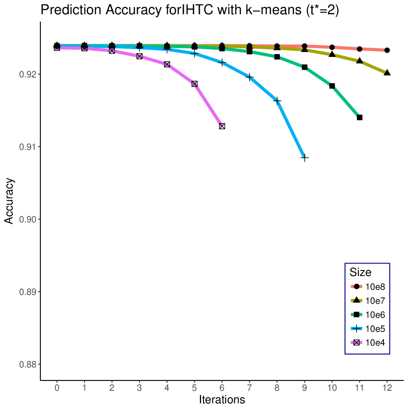
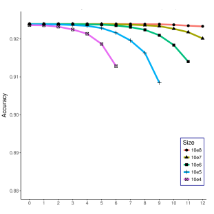
We perform IHTC with $k$-means with threshold $t^{*}=2$ and number of clusters $k=3$. The run time and memory usage are in Figure 3 and Table 1. Because we simulated data from a Gaussian mixture model, each cluster roughly should correspond to a different Gaussian distribution. Hence, we can use prediction accuracy to measure the performance of our methods. The prediction accuracy is the number of units correct clustered divided by data size $n$. The prediction accuracy for IHTC with $k$-means are in Figure 4 and Table 1. The first point of each curve (iteration $m=0$) indicates the performance without pre-processing of the data; that is $m=0$ indicates where only the original clustering algorithm is applied to the data.

From Figures 3 and 4, and from Table 1, we find that using IHTC with $k$-means decreases the runtime and memory required compared to without IHTC. After one iteration, the runtime and memory usage decreases by about half while the prediction accuracy remains the same. As the number of iterations increases, the additional improvements in runtime and memory usage decrease. After several iterations, runtime and memory usage tend to level off and prediction accuracy slowly decreases.

Iteration	Run Time (second)					Memory (Mb)					Accuracy
($m$)	$10^{4}$	$10^{5}$	$10^{6}$	$10^{7}$	$10^{8}$	$10^{4}$	$10^{5}$	$10^{6}$	$10^{7}$	$10^{8}$	$10^{4}$	$10^{5}$	$10^{6}$	$10^{7}$	$10^{8}$
0	0.143	1.613	18.773	218.43	2815	19.39	241.64	2556	27540	279346	0.9236	0.9239	0.9239	0.9239	0.9239
1	0.084	0.909	10.337	119.86	1767	8.70	99.14	1019	11097	110467	0.9236	0.9239	0.9239	0.9239	0.9239
2	0.072	0.647	7.886	97.07	1572	3.99	44.00	488	5462	54773	0.9232	0.9238	0.9239	0.9239	0.9239
3	0.058	0.550	6.975	88.52	1522	1.76	23.55	253	3104	31764	0.9225	0.9237	0.9239	0.9239	0.9239
4	0.053	0.502	6.534	83.86	1487	0.97	14.19	166	2150	21962	0.9214	0.9234	0.9238	0.9239	0.9239
5	0.053	0.497	6.332	81.46	1378	0.81	8.62	130	1761	17757	0.9187	0.9229	0.9238	0.9239	0.9239
6	0.051	0.487	6.272	80.90	1350	0.81	7.94	112	1614	16478	0.9128	0.9216	0.9235	0.9239	0.9239
7	-	0.487	6.263	80.62	1336	-	7.69	106	1560	15813	-	0.9196	0.9231	0.9238	0.9239
8	-	0.490	6.254	80.28	1305	-	7.56	105	1561	16005	-	0.9163	0.9224	0.9236	0.9239
9	-	0.490	6.243	80	1288	-	7.91	105	1574	16099	-	0.9085	0.9210	0.9234	0.9239
10	-	-	6.245	79.95	1252	-	-	106	1596	16512	-	-	0.9184	0.9227	0.9237
11	-	-	6.246	79.75	1268	-	-	109	1630	16587	-	-	0.9140	0.9218	0.9235
12	-	-	-	79.72	1247	-	-	-	1662	17036	-	-	-	0.9201	0.9233

Table 1: Cluster performance of IHTC with $K$-means ($k=3,t^{*}=2$).

Figure 3: Run time and memory usage of IHTC with $k$-means clustering ($k=3,t^{*}=2$).

Figure 4: Prediction accuracy of IHTC with $k$-means clustering ($k=3,t^{*}=2$).

4.2 IHTC with HAC

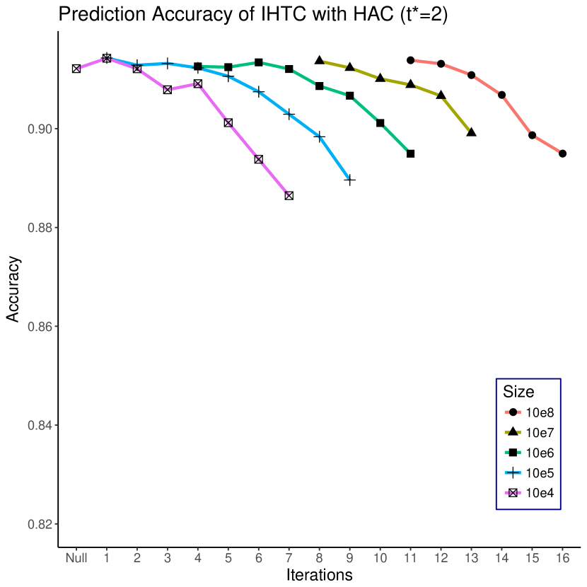
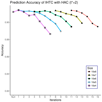
HAC is an computationally expensive algorithm. For example, if data size exceed 65,536 datapoints, the hclust function in R will throw an error. We applied IHTC with HAC and consider with respect to threshold $t^{*}=2$. Comparing the performance with pre-processing and without pre-processing, we found the reduction for runtime and memory requirement is dramatic when we apply IHTC with HAC, while prediction accuracy falls slightly. As the number iterations increase, the improvements in runtime and memory usage decrease, and after several iterations, runtime and memory tend to a certain stable value and prediction accuracy decreases. Thus, the number of iterations to perform is an unsolved problem. Figures 5 and 6, and Table 2 give the results of IHTC with HAC.

Iterations	Run Time (second)					Memory (Mb)					Accuracy
$m$	$10^{4}$	$10^{5}$	$10^{6}$	$10^{7}$	$10^{8}$	$10^{4}$	$10^{5}$	$10^{6}$	$10^{7}$	$10^{8}$	$10^{4}$	$10^{5}$	$10^{6}$	$10^{7}$	$10^{8}$
Null	5.425	-	-	-	-	796.46	-	-	-	-	0.9122	-	-	-	-
1	0.940	88.619	-	-	-	177.27	20193.0	-	-	-	0.9142	0.9143	-	-	-
2	0.220	15.755	-	-	-	20.49	3537.4	-	-	-	0.9121	0.9129	-	-	-
3	0.073	2.992	-	-	-	7.01	459.9	-	-	-	0.9079	0.9132	-	-	-
4	0.048	0.752	62.28	-	-	1.11	117.9	10891	-	-	0.9091	0.9123	0.9126	-	-
5	0.044	0.393	15.41	-	-	0.73	28.7	1940	-	-	0.9012	0.9106	0.9124	-	-
6	0.045	0.350	7.44	-	-	0.74	11.2	435	-	-	0.8938	0.9075	0.9134	-	-
7	0.044	0.343	6.21	-	-	0.74	9.3	165	-	-	0.8864	0.9029	0.9121	-	-
8	-	0.342	5.99	93.8	-	-	9.3	120	2405	-	-	0.8984	0.9086	0.9137	-
9	-	0.342	5.98	90.4	-	-	9.4	115	1648	-	-	0.8896	0.9067	0.9123	-
10	-	-	5.99	89.2	1299	-	-	118	1564	19113	-	-	0.9012	0.9101	0.9159
11	-	-	6.04	89.7	1267	-	-	123	1523	16932	-	-	0.8949	0.9089	0.9139
12	-	-	-	90.1	1288	-	-	-	1579	16760	-	-	-	0.9066	0.9131
13	-	-	-	89.9	1253	-	-	-	1604	17041	-	-	-	0.8991	0.9109
14	-	-	-	-	1272	-	-	-	-	17505	-	-	-	-	0.9068
15	-	-	-	-	1283	-	-	-	-	17784	-	-	-	-	0.8987
16	-	-	-	-	1288	-	-	-	-	18220	-	-	-	-	0.8950

Table 2: Cluster performance for IHTC with HAC ($t^{*}=2$)

Figure 5: Run time and memory usage of IHTC with HAC ($t^{*}=2$).

Figure 6: Prediction accuracy of IHTC with HAC ($k=3,t^{*}=2$).

5 Experiments

In this section, we will use our threshold clustering algorithm performance on several publicly available datasets. A brief description of each dataset can be found in Table 3. The Euclidean distance is used to measure the dissimilarity and principal component analysis (Hotelling, 1933; Friedman et al., 2001) is used for each dataset to perform feature selection. The number of classes ($k$) is chosen by the elbow of plot of within-cluster sum of squared distances for different $k$. All experiments run on a single CPU core laptop.

Name	Instances	Attributes	Classes
PM 2.5 (Havera, 2017)	41757	5	4
Credit Score (Kaggle, 2011)	120269	6	5
Black Friday (Dagdoug, 2018)	166986	7	4
Covertype (Blackard and Dean, 1999)	581012	6	7
House Price (Zillow, 2017)	2885485	5	5
Stock (Brogaard et al., 2014; Carrion, 2013)	7026593	5	7

Table 3: Data description.

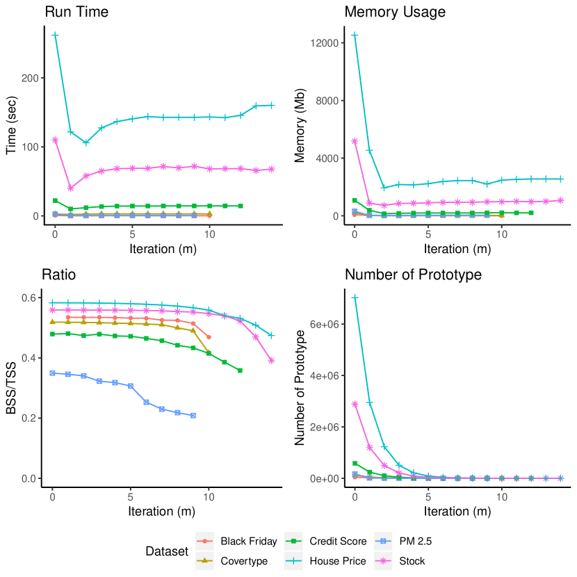
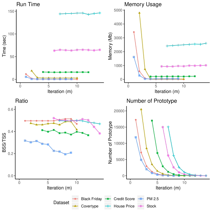
Tables 4, 5, and 6, and Figures 7 and 8 demonstrate results of IHTC with $k$-means and HAC for these datasets. Iteration $m=0$ indicates the performance when no pre-processing was conducted; only $k$-means clustering was applied to the data. BSS/TSS is the ratio of between cluster sum of squares and total sum of squares. Larger ratio value indicates better cluster performance. The number of prototypes is the size of the reduced data after $m$ iterations. We found that using IHTC with $k$-means or HAC decreases the runtime and memory required compared to without IHTC. After one iteration, the runtime and memory usage decreases by about half while preserving the value of the BSS/TSS ratio. As the number of iterations becomes large, the improvements in runtime and memory usage decrease and the BSS/TSS ratio decreases slowly.

To demonstrate the versitility of IHTC, we also consider its performance with the clustering method DBSCAN (Ester et al., 1996). The results of DBSCAN are contained in Appendix B.

Name	Run Time (second)				Memory Usage (Mb)				BSS/TSS				Number of Prototypes
	$m=0$	$m=1$	$m=2$	$m=3$	$m=0$	$m=1$	$m=2$	$m=3$	$m=0$	$m=1$	$m=2$	$m=3$	$m=0$	$m=1$	$m=2$	$m=3$
PM 2.5	0.636	0.282	0.232	0.268	71.28	25.69	3.7	5.91	0.5347	0.5346	0.5345	0.5344	41757	17281	7166	2984
Credit Score	2.902	2.046	2.696	2.904	224.55	23.9	13.95	17.65	0.5187	0.5184	0.5178	0.5169	120269	49669	20471	8456
Black Fridy	2.802	0.468	0.522	0.554	317.05	32.95	24.5	28.91	0.3493	0.3456	0.3402	0.3226	166986	11868	4914	2017
Covertype	22.244	10.184	11.968	13.562	1073.9	387.66	150.46	172.78	0.4791	0.4806	0.4741	0.4787	581012	241072	99509	41102
House Price	110.08	40.24	58.02	65.05	5178.7	881.2	726.4	859.4	0.5589	0.5589	0.5589	0.5587	2885485	1196674	496442	206332
Stock	262	121.82	105.98	127.62	12528.9	4545.9	1943.8	2169.9	0.5829	0.5828	0.5825	0.5820	7026593	2952376	1226666	508366

Table 4: Cluster performance for IHTC with $k$-means ($t^{*}=2$).

Performance	PM 2.5			Credit Score			Black Friday
	$m=1$	$m=2$	$m=3$	$m=2$	$m=3$	$m=4$	$m=1$	$m=2$	$m=3$
Run Time (second)	11.7	1.9	0.48	18.87	3.79	3.07	5.66	1.01	0.60
Memory Usage (Mb)	3420.6	588.9	79.7	4799.3	730.98	21.32	1618.94	277.87	38.44
BSS/TSS	0.4964	0.4964	0.4964	0.4746	0.4612	0.4613	0.3176	0.3024	0.3142
Number of Prototypes	17281	7166	2984	20471	8456	3508	11868	4914	2017

Table 5: Cluster performance for IHTC with HAC ($t^{*}=2$).

Performance	Covertype			House Price			Stock
	$m=4$	$m=5$	$m=6$	$m=6$	$m=7$	$m=8$	$m=7$	$m=8$	$m=9$
Run Time (second)	16.34	15.96	15.72	63.3	65.1	64.4	144.24	144.84	145.12
Memory Usage (Mb)	206.53	211.25	210.1	940.74	934.97	933.79	2415.6	2443.9	2471.9
BSS/TSS	0.4124	0.3982	0.4144	0.5213	0.5017	0.5017	0.4986	0.4945	0.4993
Number of Prototypes	17015	7015	2911	15014	6268	2598	15085	6267	2603

Table 6: Cluster performance for IHTC with HAC ($t^{*}=2$).

Figure 7: Cluster performance for IHTC with K-means.

Figure 8: Cluster performance for IHTC with HAC.

6 Discussion

Many clustering methods share one ubiquitous drawback: as the size of the data becomes massive—that is, as the number of units $n$ for the data becomes large—these methods become intractable. Even efficient implementations of these algorithms require prohibitive computational resources under massive $n$ settings. Recently, threshold clustering (TC) has been developed as a way of clustering units so that each cluster contains a pre-specified number of units and so that the maximum within-cluster dissimilarity is small. Unlike many clustering methods, TC is designed to form clustering comprised of many groups of only a few units. Moreover, the runtime and memory requirement for TC is smaller compared to other clustering methods.

In this paper, we propose using TC as an instance selection method called iterative threshold instance selection (ITIS) to efficiently and effectively reduce the size of data. Additionally, we propose coupling ITIS with other, more sophisticated clustering methods to obtain method to sufficiently scale down the size of data. and introduced IHTC that can efficiently and effectively scale down the size of data so that more sophisticated clustering methods can be applied on the reduced data.

Simulation results and application on real datasets show that implementing clustering methods with IHTC may decrease their runtime and memory usage without sacrificing the their performance. For more sophisticated clustering methods, this reduction in runtime and memory usage may be dramatic. Even for the standard implementation of $k$-means in R, one iteration of IHTC decreases the runtime and memory usage by more than half while maintaining clustering performance.

A Cluster Performance for IHTC with Varying Threshold Size

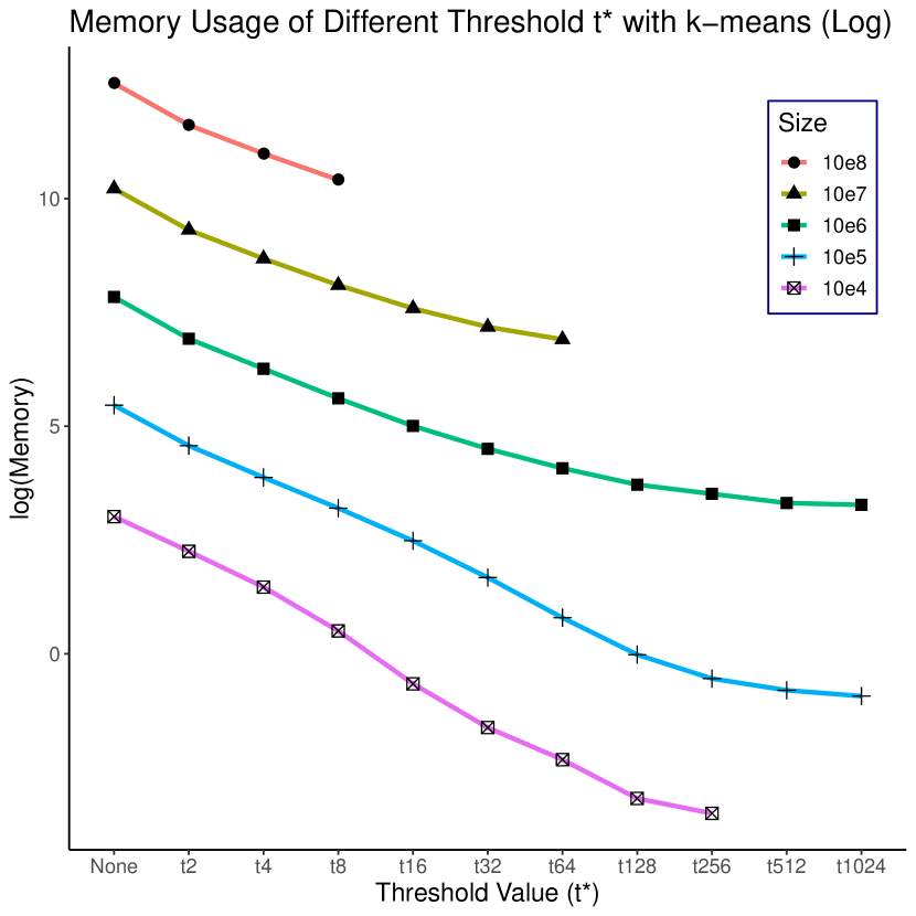
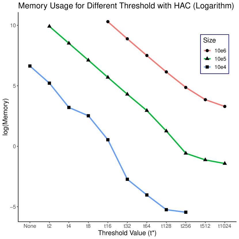
We compare the cluster performance for IHTC with varying threshold $t^{*}$ across different data size. For this example, we generate data using the multivariate Gaussian model in Section 4. We set $k=3$, $n$ is between $10^{4}$ and $10^{8}$, and perform one iteration of IHTC ($m=1$). We analyze performance across different thresholds: $t^{*}=2,4,8,16,32,64,128,256,512$ and $1024$. The runtime, memory usage and prediction accuracy for IHTC with $k$-means can be found in Figures 9 and 11, and Table 7. Figures 10 and 11, and Table 8 present the cluster performance for IHTC with HAC.

We find, that when the threshold $t^{*}$ is small, pre-processing the data with IHTC decreases runtime and memory usage compared to without pre-processing, and prediction accuracy fluctuates within a narrow range. When $t^{*}$ is large, the runtime for our method takes longer than the runtime without pre-processing. In general, across all data sizes, the runtime initially decreases before steadily increasing as $t^{*}$ increases. On the other hand, despite increasing the threshold $t^{*}$, the memory usage for IHTC with $k$-means or HAC is continually reducing. Additionally, the prediction accuracy decreases slightly with larger values of $t^{*}$.

Figure 9: Run time and memory usage of different t* with $k$-means ($k=3,m=1$).

Figure 10: Runtime and memory usage of for different threshold $t^{*}$ with HAC ($m=1$).

Figure 11: Prediction accuracy of for different threshold $t^{*}$ ($m=1$).

	Run Time (second)					Memory Usage (Mb)					Accuracy
$t^{*}$	$10^{4}$	$10^{5}$	$10^{6}$	$10^{7}$	$10^{8}$	$10^{4}$	$10^{5}$	$10^{6}$	$10^{7}$	$10^{8}$	$10^{4}$	$10^{5}$	$10^{6}$	$10^{7}$	$10^{8}$
None	0.152	1.44	17.5	214	2697	20.37	235.36	2538	27468	278617	0.9238	0.9240	0.9239	0.9239	0.9239
2	0.109	0.75	9.6	118	1640	9.50	96.73	1014	11085	110919	0.9237	0.9240	0.9239	0.9239	0.9239
4	0.067	0.53	7.7	98	1540	4.33	48.17	525	5898	59288	0.9236	0.9240	0.9239	0.9239	0.9239
8	0.070	0.56	9.4	119	2137	1.65	24.50	274	3293	33316	0.9233	0.9239	0.9239	0.9239	0.9239
16	0.099	0.86	15.5	197	-	0.52	11.97	149	1975	-	0.9230	0.9238	0.9239	0.9239	-
32	0.161	1.64	29.8	467	-	0.20	5.34	90	1314	-	0.9219	0.9238	0.9239	0.9239	-
64	0.297	3.54	62.3	1032	-	0.10	2.21	59	999	-	0.9203	0.9233	0.9238	0.9239	-
128	0.658	8.72	200.8	-	-	0.04	0.98	41	-	-	0.9174	0.9231	0.9238	-	-
256	1.565	37.38	546.4	-	-	0.03	0.58	34	-	-	0.9086	0.9221	0.9238	-	-
512	-	100.56	1585	-	-	-	0.45	27	-	-	-	0.9204	0.9235	-	-
1024	-	384.17	5541	-	-	-	0.39	26	-	-	-	0.9162	0.9231	-	-

Table 7: Cluster performance for iterate once with $k$-means ($k=3,m=1$).

	Run Time (s)			Memory Usage (Mb)			Accuracy
$t^{*}$	$10^{4}$	$10^{5}$	$10^{6}$	$10^{4}$	$10^{5}$	$10^{6}$	$10^{4}$	$10^{5}$	$10^{6}$
Null	5.366	-	-	764.5	-	-	0.9111	-	-
2	0.984	115.9	-	184.8	20196	-	0.9113	0.9140	-
4	0.246	22.59	-	24.84	4992	-	0.9113	0.9127	-
8	0.095	5.491	-	12.46	1230	-	0.9118	0.9135	-
16	0.091	2.047	165.8	1.720	298.4	29701	0.9106	0.9131	0.9075
32	0.153	2.035	65.59	0.066	73.78	7207	0.9093	0.9127	0.9117
64	0.297	3.919	69.05	0.018	19.17	1813	0.9078	0.9123	0.9125
128	0.697	9.522	201.3	0.005	3.517	466.2	0.9076	0.9121	0.9143
256	1.662	40.73	534.3	0.004	0.561	130.2	0.9056	0.9105	0.9112
512	-	105.2	1630	-	0.325	47.29	-	0.9096	0.9139
1024	-	401.4	6042	-	0.241	26.97	-	0.9049	0.9115

Table 8: Simulation result for different threshold $t^{*}$ with HAC ($m=1$).

B Experiment for IHTC with DBSCAN

Table 9 shows the result on the four datasets with the fewest instances. The parameters $\epsilon$ and $Minpts$ are decided by subsample of size 1000 of each dataset with a 10-fold cross-validation method. Comparing the performance for DBSCAN with and without IHTC, we find that IHTC with DBSCAN has shorter runtime but higher memory usage than DBSCAN itself. Total sum of squares (TSS) is equal to between-cluster sum of squares (BSS) plus within-cluster sum of squares. Higher ratio of BSS and TSS indicates the clusters are more compact. We found that the ratio of BSS and TSS is higher when applying IHTC, which shows our method has comparable clustering performance.

Name	Run Time (second)			Memory Usage (Mb)			BSS/TSS
	$m=0$	$m=1$	$m=2$	$m=0$	$m=1$	$m=2$	$m=0$	$m=1$	$m=2$
PM 2.5	3.96	0.9	0.26	0.8	0.4	0.2	0.5036	0.5627	0.5336
Credit Score	25.78	4.16	2.66	3.3	1.2	38	0.4731	0.6015	0.6441
Black Fridy	9.26	0.64	0.56	13.5	62.1	66.2	0.3103	0.9657	0.9985
Covertype	233.9	223.8	231.4	13.3	15.6	15.6	0.1785	0.1785	0.1785

Table 9: Cluster performance for IHTC with DBSCAN ($t^{*}=2$).

C Graph theory definitions

Let $G=(V,E)$ denote an undirected graph.

Definition 1

Vertices $i$ and $j$ are adjacent in $G$ if the edge $ij\in E$.

Definition 2

A set of vertices $I\subseteq V$ is independent in $G$ if no vertices in the set are adjacent to each other. That is, for all $i,j\in I$, $ij\notin E$.

Definition 3

An independent set of vertices $I$ in $G$ is maximal if, for any additional vertex $i\in V$, the set $i\cup I$ is not independent. That is, for all $i\in V\setminus I$, there exists $j\in I$ such that $ij\in E$.

Definition 4

For $i,j\in V$, a walk from $i$ to $j$ of length $m$ in $G$ is a sequence of $m+1$ vertices $(i=i_{0},i_{1},\ldots,i_{m}=j)$ such that the edge $i_{\ell-1}i_{\ell}\in E$.

Note that, if $(i=i_{0},i_{1},i_{2},\cdots,i_{m}=j)$ is a walk of length $m$ from $i$ to $j$ and the edge weights of $G$ satisfy the triangle inequality (1), then the weight $w_{ij}$ satisfies the inequality:

$$w_{ij}\leq m\max_{\ell}(w_{i_{\ell-1}i_{\ell}}).$$ (3)

Definition 5

The $d^{\text{th}}$ power of $G$, denoted $G^{d}=(V,E^{d})$, is a graph such that an edge $ij\in E^{d}$ if and only if there is a walk from $i$ to $j$ of length at most $d$ in $G$.

Definition 6

The $k$-nearest-neighbors subgraph of $G$ is a subgraph $NG_{k}=(V,NE_{k})$ where an edge $ij\in NE_{k}$ if and only if $j$ is one of the $k$ closest vertices to $i$ or $i$ is one of the $k$ closest vertices to $j$. Rigorously, for a vertex $i$, let $i_{(\ell)}$ denote the vertex that corresponds to the $\ell^{\text{th}}$ smallest value of $w_{ij},ij\in E$, where ties are broken arbitrarily: $w_{ii_{(1)}}\leq w_{ii_{(2)}}\leq\cdots\leq w_{ii_{(m)}}$. Then

$$NE_{k}\equiv\left\{ij\in E:j\in(i_{(\ell)})_{\ell=1}^{k}\text{ or }i\in(j_{(\ell)})_{\ell=1}^{k}\right\}.$$ (4)

References

- Arthur and Vassilvitskii (2007) David Arthur and Sergei Vassilvitskii. k-means++: The advantages of careful seeding. In Proceedings of the eighteenth annual ACM-SIAM symposium on Discrete algorithms, pages 1027–1035. Society for Industrial and Applied Mathematics, 2007.
- Blackard and Dean (1999) Jock A. Blackard and Denis J. Dean. Comparative accuracies of artificial neural networks and discriminant analysis in predicting forest cover types from cartographic variables, 1999.
- Blum and Langley (1997) Avrim L Blum and Pat Langley. Selection of relevant features and examples in machine learning. Artificial intelligence, 97(1-2):245–271, 1997.
- Brogaard et al. (2014) Jonathan Brogaard, Terrence Hendershott, and Ryan Riordan. High-frequency trading and price discovery. The Review of Financial Studies, 27(8):2267–2306, 2014.
- Carrion (2013) Allen Carrion. Very fast money: High-frequency trading on the nasdaq. Journal of Financial Markets, 16(4):680–711, 2013.
- Cukier (2010) Kenneth Cukier. Data, data everywhere: A special report on managing information. Economist Newspaper, 2010.
- Dagdoug (2018) Mehdi Dagdoug. Black friday: A study of sales trough consumer behaviours, 2018. URL https://www.kaggle.com/mehdidag/black-friday.
- Ester et al. (1996) Martin Ester, Hans-Peter Kriegel, Jörg Sander, Xiaowei Xu, et al. A density-based algorithm for discovering clusters in large spatial databases with noise. In Kdd, volume 96, pages 226–231, 1996.
- Firdaus and Uddin (2015) Sabhia Firdaus and Md Ashraf Uddin. A survey on clustering algorithms and complexity analysis. International Journal of Computer Science Issues (IJCSI), 12(2):62, 2015.
- Fränti and Kivijärvi (2000) Pasi Fränti and Juha Kivijärvi. Randomised local search algorithm for the clustering problem. Pattern Analysis & Applications, 3(4):358–369, 2000.
- Fränti et al. (1997) Pasi Fränti, Juha Kivijärvi, Timo Kaukoranta, and Olli Nevalainen. Genetic algorithms for large-scale clustering problems. The Computer Journal, 40(9):547–554, 1997.
- Friedman et al. (2001) Jerome Friedman, Trevor Hastie, and Robert Tibshirani. The elements of statistical learning, volume 1. Springer series in statistics Springer, Berlin, 2001.
- Friedman et al. (1976) Jerome H Friedman, Jon Louis Bentley, and Raphael Ari Finkel. An algorithm for finding best matches in logarithmic time. ACM Trans. Math. Software, 3(SLAC-PUB-1549-REV. 2):209–226, 1976.
- Frnti et al. (1998) P Frnti, J Kivijrvi, and OLLI Nevalainen. Tabu search algorithm for codebook generation in vector quantization. Pattern Recognition, 31(8):1139–1148, 1998.
- Hartigan and Wong (1979) John A Hartigan and Manchek A Wong. Algorithm as 136: A k-means clustering algorithm. Journal of the Royal Statistical Society. Series C (Applied Statistics), 28(1):100–108, 1979.
- Hastie et al. (2009) Trevor Hastie, Robert Tibshirani, and Jerome Friedman. Unsupervised learning. In The elements of statistical learning, pages 485–585. Springer, 2009.
- Havera (2017) David Havera. Beijing pm2.5 data data set, 2017. URL https://www.kaggle.com/djhavera/beijing-pm25-data-data-set/activity.
- Higgins et al. (2016) Michael J Higgins, Fredrik Sävje, and Jasjeet S Sekhon. Improving massive experiments with threshold blocking. Proceedings of the National Academy of Sciences, 113(27):7369–7376, 2016.
- Hochbaum and Shmoys (1986) Dorit S Hochbaum and David B Shmoys. A unified approach to approximation algorithms for bottleneck problems. Journal of the ACM (JACM), 33(3):533–550, 1986.
- Hotelling (1933) Harold Hotelling. Analysis of a complex of statistical variables into principal components. Journal of educational psychology, 24(6):417, 1933.
- Jain et al. (1999) Anil K Jain, M Narasimha Murty, and Patrick J Flynn. Data clustering: a review. ACM computing surveys (CSUR), 31(3):264–323, 1999.
- Jordan and Mitchell (2015) Michael I Jordan and Tom M Mitchell. Machine learning: Trends, perspectives, and prospects. Science, 349(6245):255–260, 2015.
- Kaggle (2011) Kaggle. Give me some credit. Website, 2011. URL https://www.kaggle.com/c/GiveMeSomeCredit/data. last checked: 12.08.2018.
- Knuth (1998) Donald Ervin Knuth. The art of computer programming: sorting and searching, volume 3. Pearson Education, 1998.
- Kurita (1991) Takio Kurita. An efficient agglomerative clustering algorithm using a heap. Pattern Recognition, 24(3):205–209, 1991.
- Leyva et al. (2015) Enrique Leyva, Antonio González, and Raúl Pérez. Three new instance selection methods based on local sets: A comparative study with several approaches from a bi-objective perspective. Pattern Recognition, 48(4):1523–1537, 2015.
- Liu and Motoda (1998) Huan Liu and Hiroshi Motoda. Feature extraction, construction and selection: A data mining perspective, volume 453. Springer Science & Business Media, 1998.
- Liu and Motoda (2002) Huan Liu and Hiroshi Motoda. On issues of instance selection. Data Mining and Knowledge Discovery, 6(2):115–130, 2002.
- Lloyd (1982) Stuart Lloyd. Least squares quantization in pcm. IEEE transactions on information theory, 28(2):129–137, 1982.
- Olvera-López et al. (2007) J Arturo Olvera-López, J Ariel Carrasco-Ochoa, and J Francisco Martínez-Trinidad. Object selection based on clustering and border objects. In Computer Recognition Systems 2, pages 27–34. Springer, 2007.
- Olvera-López et al. (2008) J Arturo Olvera-López, J Ariel Carrasco-Ochoa, and J Fco Martínez-Trinidad. Prototype selection via prototype relevance. In Iberoamerican Congress on Pattern Recognition, pages 153–160. Springer, 2008.
- Olvera-López et al. (2010) J Arturo Olvera-López, J Ariel Carrasco-Ochoa, J Francisco Martínez-Trinidad, and Josef Kittler. A review of instance selection methods. Artificial Intelligence Review, 34(2):133–143, 2010.
- Plasencia-Calaña et al. (2014) Yenisel Plasencia-Calaña, Mauricio Orozco-Alzate, Heydi Méndez-Vázquez, Edel García-Reyes, and Robert PW Duin. Towards scalable prototype selection by genetic algorithms with fast criteria. In Joint IAPR International Workshops on Statistical Techniques in Pattern Recognition (SPR) and Structural and Syntactic Pattern Recognition (SSPR), pages 343–352. Springer, 2014.
- Pooja (2013) Saroj Ratnoo Pooja. A comparative study of instance reduction techniques. In Proceedings of 2nd International Conference on Emerging Trends in Engineering and Management, ICETEM. Citeseer, 2013.
- Raicharoen and Lursinsap (2005) Thanapant Raicharoen and Chidchanok Lursinsap. A divide-and-conquer approach to the pairwise opposite class-nearest neighbor (poc-nn) algorithm. Pattern recognition letters, 26(10):1554–1567, 2005.
- Riquelme et al. (2003) José C Riquelme, Jesús S Aguilar-Ruiz, and Miguel Toro. Finding representative patterns with ordered projections. Pattern Recognition, 36(4):1009–1018, 2003.
- Savje et al. (2017) Fredrik Savje, Michael Higgins, and Jasjeet Sekhon. scclust: Size-Constrained Clustering, 2017. URL https://CRAN.R-project.org/package=scclust. R package version 0.1.1.
- Sullivan (2015) Danny Sullivan. Google still doing at least 1 trillion searches per year. Retrieved September, 29:2015, 2015.
- University (2018) Kansas State University. Acknowledging use of beocat resources and/or personnel in publications, 2018. URL https://support.beocat.ksu.edu/BeocatDocs/index.php/Policy.
- Vaidya (1989) Pravin M Vaidya. An algorithm for the all-nearest-neighbors problem. Discrete & Computational Geometry, 4(2):101–115, 1989.
- Ward Jr (1963) Joe H Ward Jr. Hierarchical grouping to optimize an objective function. Journal of the American statistical association, 58(301):236–244, 1963.
- Zillow (2017) Zillow. Zillow prize: Zillow’s home value prediction (zestimate), 2017. URL https://www.kaggle.com/c/zillow-prize-1.