Preliminary Results in Current Profile Estimation and Doppler-aided Navigation
for Autonomous Underwater Gliders

Abstract

This paper describes the development and experimental results of navigation algorithms for an autonomous underwater glider (AUG) that uses an on-board acoustic Doppler current profiler (ADCP). AUGs are buoyancy-driven autonomous underwater vehicles that use small hydrofoils to make forward progress while profiling vertically. During each dive, which can last up to 6 hours, the Seaglider AUG used in this experiment typically reaches the depth of 1000 m and travels 3-6 km horizontally through the water, relying solely on dead-reckoning. Horizontal through-the-water (TTW) progress of AUG is 20-30 cm/s, which is comparable to the speed of the stronger ocean currents. Underwater navigation of an AUG in the presence of unknown advection therefore presents a considerable challenge. We develop two related formulations for post-processing. Both use ADCP observations, through the water velocity estimates, and GPS fixes to estimate current profiles. However, while the first solves an explicit inverse problem for the current profiles only, the second solves a deconvolution problem that infers both states and current profiles using a state-space model.

Both approaches agree on their estimates of the ocean current profile through which the AUG was flown using measurements of current relative to the AUG from the ADCP, and estimates of the AUGs TTW velocity from a hydrodynamic model. The result is a complete current profile along the AUGs trajectory, as well as over-the-ground (OTG) velocities for the AUG that can be used for more accurate subsea positioning. Results are demonstrated using 1 MHz ADCP data collected from a Seaglider AUG deployed for 49 days off the north coast of Alaska during August and September 2017. The results are compared to ground truth data from the top 40 meters of the water column, from a moored, upward-facing 600 kHz ADCP. Consequences of the state-space formulation are discussed in the Conclusions section.

I Introduction

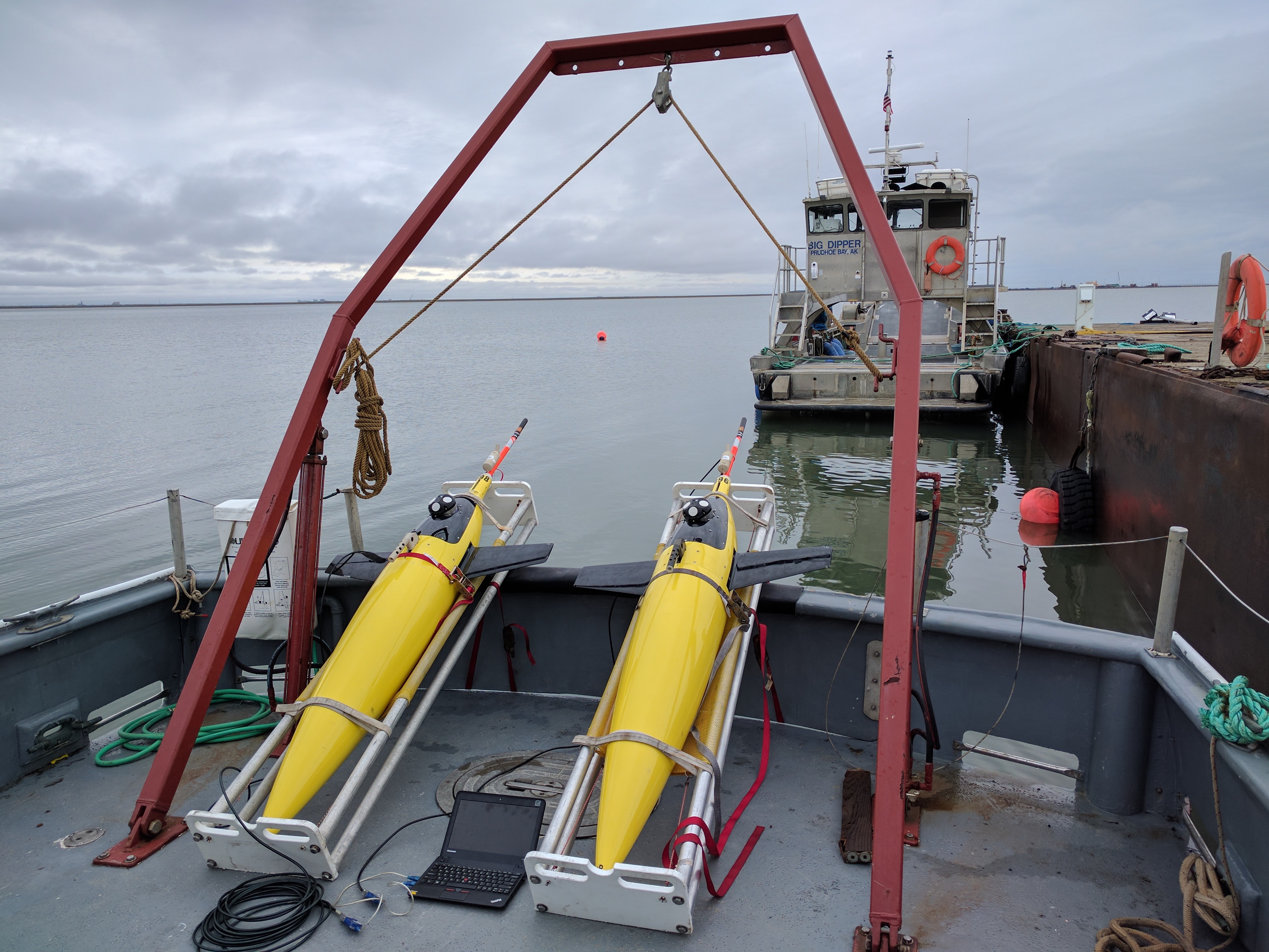
The goal of this work is to simultaneously estimate a) absolute (Earth-referenced) ocean velocity profile, and b) the absolute autonomous underwater glider (AUG) path over the bottom, based on on-board acoustic Doppler current profiler (ADCP) observations of relative current velocity profiles. Figure 1 shows two Seagliders with upward-facing ADCPs mounted in the aft fairing.

Figure 1: Ready for launch, Seagliders SG196 and SG198 are loaded on the R/V Ukpik in Prudhoe Bay, AK, with the upward-facing ADCPs visible where they are installed in the aft fairing.

The main challenge of AUG-based ADCP velocity profiling is that each velocity profile is measured relative to the through-the-water (TTW) motion of the glider, as opposed to the earth referenced glider velocity. The AUG’s TTW velocity can be inferred from the AUG dynamic model, but is subject to uncertainty because the model is based on steady state flight and doesn’t take roll into account. This lack of a georeferenced platform velocity requires a simultaneous estimation of current and glider TTW velocity using all available data—ADCP velocity profiles, surrounding water density, glider buoyancy engine state, glider attitude and angle of attack, glider depth, and GPS positions at the start and end of the dive.

Here we describe two different frameworks for performing this estimation—a linear global inverse, and a flexible state space approach. In this initial work, we use a pre-computed estimate of the glider TTW velocity from the hydrodynamic model for both methods. The overarching future goal is to use the flexibility of the state-space model to include the nonlinear hydrodynamic model and nonlinear range measurements as part of the approach.

II Background

Historically, ADCP measurements were made from ships with with relatively low frequency systems (70 kHz) or from moorings with low or mid-frequency instruments (300 kHz). The 300 kHz ADCPs are also common on large underwater vehicles, in particular instruments that can be used as a Doppler velocity log to provide “bottom lock”—i.e., vehicle velocity relative to the seafloor [1] or, in some specialized cases, the underside of ice [2].

To provide better resolution of deep currents from shipboard measurements, lowered ADCP methods were developed using overlapping shear traces from a higher frequency (typically 150 or 300 kHz) ADCP lowered from a (relatively) stationary ship. The shear traces are then used to reconstruct the full current profile. The two main lowered ADCP processing frameworks are the shear method, originally described by [3, 4], and the velocity inversion method [5].

In the last 10 years, there has been increased interest in using ADCPs from autonomous underwater vehicles to characterize the currents between the surface and the seafloor and to close the gap of uncertainty in vehicle drift between when GPS is available at the surface and bottom lock is obtained within range of the seafloor [6, 7, 8].

Aided by the development of very high frequency ADCPs (1 MHz) specifically for autonomous underwater gliders, the two main lowered ADCP processing frameworks—the shear method and the inversion method—have been modified to estimate depth-varying current profiles from gliders by [9] and [10, 11] respectively. A related, but distinctly different method based on non-linear objective mapping of ADCP shear has been also developed by [12]. In all implementations ([9, 11, 12]), the authors needed to contend with the limitation of Slocum and Spray glider ADCPs that only collect data during one half of the dive (either ascending or descending).

Our contribution builds on and extends the velocity inversion method with several key innovations. We use current data from the entire dive (as opposed to just during descent), which is crucial for multi-hour dives where, as we show, the current profiles on descent versus ascent differ significantly. We then explicitly separate the over-the-ground glider velocity into the drift velocity (as a result of advection), and the glider’s horizontal through-the-water velocity. This enables us to directly incorporate hydrodynamic model velocity estimates and independently control the smoothness regularization of the different velocity components.

III Finding the Current Profile by Inversion

In this section we develop an approach to use (1) on-board ADCP observations of relative current velocity profiles, (2) dive start and end GPS coordinates and (3) a measure of through the water (TTW) velocity obtained from the glider to simultaneously estimate (a) absolute (Earth-referenced) ocean velocity profile, and (b) the glider path through the water. We present the derivation for a scalar velocity $v$, which can be understood to be either one of the velocity components $(u,v)$, or a complex-number representation of velocity, $u+iv$.

III-A Formulation of the inverse problem

Similar to [5, 10], glider-borne ADCP observations of horizontal currents are considered to be a sum of three unknown components:

$$u^{a}(z,t)=u^{o}(z)-u^{g}(t)+\epsilon(z,t),$$

where

• $u^{o}$ is the absolute ocean velocity

• $u^{g}$ is the over-the-ground (OTG) velocity of the glider platform

• $\epsilon$ is the ADCP measurement noise.

Here, we separate the OTG glider velocity into the drift velocity $u^{d}=u^{o}(z^{g}(t))$, equal to the ocean velocity at the glider depth $z^{g}$, and the glider horizontal TTW ”propulsion” speed $u^{p}$, which is determined by the glider control and its flight dynamics:

$$u^{g}(t)=u^{o}(z^{g}(t))+u^{p}(t).$$

Thus the inverse problem is to obtain $u^{o}(z)$ and $u^{g}(t)$ such that the discrepancy with the observed values of $u^{a}$ are minimized,

$$\min{\|u^{a}(z,t)-(u^{o}(z)-u^{o}(z^{g}(t))-u^{p}(t))\|_{2}^{2}}.$$ (1)

This formulation uses the least squares loss, corresponding to a Gaussian assumption on the noise $\epsilon$. More robust losses are of interest and will be studied in future work.

This formulation is more complex than that of [10], as it requires interpolation of ocean velocity onto the glider location ($u^{o}(z^{g}(t))$), but it allows explicit treatment of the glider state. Additionally, applying smoothness regularization to $u^{p}$ as discussed below is more appropriate than to $u^{g}$.

III-B Discrete formulation

We consider a set of individual ADCP observations $u^{a}_{ij}=u^{a}(z_{ij},t_{j})$ at depth cells $z_{ij}$ and times $t_{j}$, with the $i\in[1,I]$ being the ADCP range cell index, and $j\in[1,J]$ being the sample time (ping) index. All the valid observations form an observation column vector

$$u^{a}=[u^{a}_{1}...u^{a}_{k}]^{\top},$$

where the index $k\in[1,K],K\leq IJ$ enumerates valid observations. The vectors $[z_{k}]$ and $[t_{k}]$ represent the corresponding depth and time coordinates of the $k$-th valid observation.

The unknown state vector

$$x=\begin{bmatrix}{u^{g}}\\ u^{o}\end{bmatrix}$$

consists of a vector of the unknown glider OTG velocities

$${u^{g}}=[u^{g}_{1}...u^{g}_{M}]^{\top}$$

defined on a temporal grid $\hat{t}_{m},m\in[1,M]$, and a vector of the unknown ocean velocities

$$u^{o}=[u^{o}_{1}...u^{o}_{L}]^{\top}$$

defined on a regular vertical grid $\hat{z}_{l}=(l-1)\Delta\hat{z},l\in[1,L]$. For convenience, the temporal grid $\hat{t}_{m}$ is taken to be a superset of the sample times $t_{j}$, with the extra intervals added during the gaps in the ADCP record (at the beginning and the end of the dive, as well as during a brief intermission at the bottom of the dive); the spacing of the extra intervals is set to the average ADCP sampling interval. Discrete formulation of the ADCP sampling problem (1) then becomes

$$u^{a}=-H^{t}u^{g}+H^{z}u^{0}+\epsilon,$$

where $\epsilon$ is the noise vector. The matrix operator $H^{t}$ represents temporal interpolation from the time grid $\{\hat{t}_{m}\}$ onto the sampling times $\{t_{k}\}$, and $H^{z}$ represents spatial interpolation from the vertical grid $\{\hat{z}_{l}\}$ onto $\{z_{k}\}$. Since $\{t_{k}\}\subset\{\hat{t}_{m}\}$ by construction, $H^{t}$ is simply a subsampling matrix,

$$H^{t}_{km}=\begin{cases}1,&\text{if }t_{k}=\hat{t}_{m}\\ 0,&\text{otherwise }\end{cases}.$$

The formulation of vertical interpolation matrices depends on the chosen interpolation method. Visbeck [5] method is equivalent to the nearest-neighbor interpolation. Here, we employ linear interpolation, corresponding to a matrix operator

$$H^{z}_{kl}=\begin{cases}1-(\hat{z}_{l}-z_{k})/\Delta\hat{z},&\hat{z}_{l-1}\leq z_{k}<\hat{z}_{l}\\ 1-(z_{k}-\hat{z}_{l})/\Delta\hat{z},&\hat{z}_{l}\leq z_{k}<\hat{z}_{l+1}\\ 0,&\text{otherwise.}\end{cases}$$

III-C Additional Regularization

The inversion framework balances physical knowledge of the glider’s motion (such as start- and end-of-dive GPS fixes) against assumptions about the physical environment, including smoothness of current profiles in time and space.

Start- and End-of-Dive GPS: GPS fixes before and after the dive provide tie-points on the integral $\int u^{g}dt$ over the duration of the dive. The discrete formulation of these relationships is given by

$$Sx\approx s,$$

where $s$ is the scalar (complex) horizontal displacement between the two GPS fixes, $S=\begin{bmatrix}w&0\end{bmatrix},$ and $w$ represents the weights corresponding to trapezoidal rule integration,

$$w_{m}=\begin{cases}0.5(\hat{t}_{2}-\hat{t}_{1}),&m=1\\ 0.5(\hat{t}_{m+1}-\hat{t}_{m-1}),&1<m<M\\ 0.5(\hat{t}_{M}-\hat{t}_{M-1}),&m=M\end{cases}$$

Glider Velocity: A measure of the glider’s TTW velocity, such as that provided by the glider hydrodynamic model, can be used to provide a constraint on $u^{p}$(t) in (1). Discrete formulation of this constraint is

$$u^{p}=-H^{t}u^{g}+H^{z0}u^{o}+\epsilon,$$

where $u^{p}$ is the TTW velocity predicted by the hydrodynamic model, and $H^{z0}$ represents spatial interpolation of ocean velocity profile onto the glider depth (so that $H^{z0}x$ is the glider drift speed); this matrix is constructed in the same way as $H^{z}$. The relative confidence, within the model, of these measurements compared to the ADCP measurements can be controlled by adjusting the relative magnitude of the noise vectors $\epsilon$ for the two measurements. As is demonstrated and discussed in the Results section, however, understanding the subtleties of how to weight the constraints is still a work in progress.

Smoothness Regularization: Additionally, we require both the ocean and the glider velocities to be smooth, which is equivalent to minimization of ${D_{2}u^{g}}$, and ${D_{2}u^{o}}$ where $D_{2}$ are the second derivative operators of the appropriate sizes,

$$D_{2}=\begin{bmatrix}1&-2&1&0&\cdots&0\\ 0&1&-2&1&\\ \vdots&&&\ddots&\ddots\\ 0&\cdots&0&1&-2&1\end{bmatrix}.$$

Subtleties of Regularization: Ideally, we want to solve an inverse problem that is aware of both the vehicle dynamics and control and the ADCP observations, because this is the only way to make a self-consistent estimate. The challenge, as mentioned above with the glider velocity estimates in particular, is that measurements are inherently noisy, often biased, and optimally choosing the relative weighting between measurements is still a work in progress.

In the extreme case, if we had a perfect hydrodynamic model, we would not need the inverse at all, as we would know the TTW velocity at any moment (based solely on the buoyancy and pitch control), and therefore would have absolute ocean velocity estimates from every trace. At the other extreme, if the ADCP measurements were perfect and extended close to the vehicle, we would have a direct measure of the TTW velocity from that information alone and would not need the dynamic model.

In reality, the ADCP is noisy and has gaps (notably, the blanking distance). And without the hydrodynamic model, we can’t distinguish between the legitimate accelerations due to AUG control (which should be kept) and spurious accelerations arising from ADCP noise (which should be eliminated)—and we would be forced to either keep both, or eliminate both, which is suboptimal.

III-D Least-Squares Formulation

The final least-squares problem formulation is given by

$$\min_{x}{\|{Gx-d}\|_{2}^{2}},$$

where

$$G=\begin{bmatrix}-H^{t}&H^{z}\\ w&0\\ -H^{t}&H^{z0}\\ r_{o}D_{2}&0\\ 0&r_{g}D_{2}\end{bmatrix},\qquad d=\begin{bmatrix}{u^{a}}\\ s\\ u^{p}\\ 0\\ 0\end{bmatrix},$$

and $r_{o}$ and $r_{g}$ are regularization parameters. The solution is given by

$$x=(G^{\top}G)^{-1}G^{\top}d,$$

and can be computed in a more efficient manner (e.g., using a QR decomposition aware of the block structure of $G$).

III-E Modification: two-profile solution

The ocean velocity profile is expected to change over the duration of the dive. Therefore, it may be reasonable to seek two ocean velocity profiles $u^{d}$ and $u^{u}$, corresponding to the descent and asent. The state vector and the observation matrix then become

$$x=\begin{bmatrix}{u^{g}}\\ u^{d}\\ u^{u}\end{bmatrix},$$

$$H=\begin{bmatrix}&-H^{t}&|&H^{zd}&|&H^{zu}&\end{bmatrix},$$

where the interpolation matrices $H^{zd}$ and $H^{zu}$ are constructed as $H^{z}$ before, except that only those rows of $H^{zd}$ that correspond to the downcast $z_{k}$ are non-zero, and vise versa.

An additional constraint is necessary, requiring the ocean velocity profiles to match at the bottom end, i.e.

$$\begin{bmatrix}0&e_{n}^{\top}&-e_{n}^{\top}\end{bmatrix}x=0.$$

where $e_{n}$ is the elementary vector with $1$ in the last entry.

The modified system is given by

$$\min_{x}{\|{Gx-d}\|_{2}^{2}},$$

where

$$G=\begin{bmatrix}-H^{t}&H^{zd}&H^{zu}\\ w&0&0\\ -H^{t}&H^{z0d}&H^{z0u}\\ r_{o}D_{2}&0&0\\ 0&r_{g}D_{2}&r_{g}D_{2}\end{bmatrix},\qquad d=\begin{bmatrix}{u^{a}}\\ s\\ u^{p}\\ 0\\ 0\end{bmatrix},$$

For shorter dives, assuming identical current profiles on ascent and descent may be a reasonable assumptions. For the data collected over multi-hour dives, however, as we show, there can be significant deviation in the current profile during descent and ascent, and we use the two-profile solution.

IV Deconvolving Glider State and Current Profile: State-Space Approach

In this section, we propose a state-space model that fuses available information (ADCP current profiles, GPS coordinates, and measure of smoother velocities) to simultaneously infer the states of the glider together with current profile estimation. The formulation uses identical information to that used in Section III. However, the main innovation here is to use a more detailed navigation model, with a view toward simultaneously solving the current mapping and glider localization problems. A direct consequence of this is an updated estimate of the state variables of the glider, along with the estimates of the current profile.

IV-A Glider State-Space Model

We start by constructing a linear four-dimensional state-space model for the glider positions and their derivatives (OTG velocity):

$$x_{k} :=\begin{bmatrix}e^{g}_{k}&n^{g}_{k}&\dot{e}^{g}_{k}&\dot{n}^{g}_{k}\end{bmatrix}^{T},$$ (2)

$$x_{k+1} =G_{k}x_{k}+\epsilon_{k},\quad\epsilon_{k}\sim\mathcal{N}(0,Q_{k})$$

$$z_{k} =H_{k}x_{k}+\nu_{k},\quad\nu_{k}\sim\mathcal{N}(0,R_{k}),\quad\text{for }k=1,N$$

$$\quad G_{k} =\begin{bmatrix}1&0&\Delta t_{k}&0\\ 0&1&0&\Delta t_{k}&\\ 0&0&1&0\\ 0&0&0&1\end{bmatrix},H_{k}=\begin{bmatrix}1&0&0&0\\ 0&1&0&0\end{bmatrix}$$

The four states are east/north over-the-ground (OTG) velocities and their approximate integrals. The only measurements used here are the GPS position fixes at the beginning and end of the dive. A separate term is added later to compare OTG velocities with (measured) TTW velocities.

The state-space model (2) does not force smoothness of the velocities, unlike the previous section. The full-state block bi-diagonal process-discrepancy matrix $G$, and block diagonal matrices $H,Q,R$ are

$$G=\begin{bmatrix}I&0&&\\ -G_{2}&I&\ddots&\\ &\ddots&\ddots&0\\ &&-G_{N}&I\end{bmatrix},\quad H=\begin{bmatrix}H_{1}&0&&\\ 0&\ddots&\ddots&\\ &\ddots&\ddots&0\\ &&0&H_{N}\end{bmatrix}$$

$$Q=\begin{bmatrix}Q_{1}&0&&\\ 0&\ddots&\ddots&\\ &\ddots&\ddots&0\\ &&0&Q_{N}\end{bmatrix},\quad R=\begin{bmatrix}R_{1}&0&&\\ 0&\ddots&\ddots&\\ &\ddots&\ddots&0\\ &&0&R_{N}\end{bmatrix}$$

We also introduce notation for the full state $X$, measurements $z$, and initial state $w$:

$$x=\begin{bmatrix}x_{1}\\ x_{2}\\ \vdots\\ x_{N}\end{bmatrix},\quad z=\begin{bmatrix}z_{1}\\ z_{2}\\ \vdots\\ z_{N}\end{bmatrix},\quad w=\begin{bmatrix}x_{0}\\ 0\\ \vdots\\ 0\end{bmatrix}$$

The Kalman smoother estimate for the velocities (and their derivatives) from direct observations would be obtained by solving the single least squares problem

$$\min_{x}||Gx-w||^{2}_{Q^{-1}}+||Hx-z||^{2}_{R^{-1}}$$

IV-B ADCP Measurements

We now consider unknown current profiles $c_{u}$ and $c_{v}$, which connect to the glider states in the previous sections via the simple equations

$$c_{u}=\dot{e}^{g}+z^{o}_{u}+\epsilon_{cu}$$

$$c_{v}=\dot{n}^{g}+z^{o}_{v}+\epsilon_{cv}$$

The additional decision variables $c_{u},c_{v}$ are indexed by depth. The model linking the ADCP observations to current profiles and states is given by

$$z^{o}_{u} =A_{c}c_{u}-A_{u}x+\epsilon_{cu}$$

$$z^{o}_{v} =A_{c}c_{v}-A_{v}x+\epsilon_{cv}$$

where $A_{u},A_{v}$ select out the OTG velocities at the time the measurements were taken and $A_{c}$ selects out the depths for the given measurement.

Depending on the discretization of $c_{u},c_{v}$, there may be depths without associated measurements. To estimate currents at these depths and to smooth out the final ocean velocity estimate we impose regularization terms on $c_{u}$ and $c_{v}$:

$$R(c_{u},c_{v}):=\sum_{i=1}^{N-1}({c_{u}}_{i}-{c_{u}}_{i+1})^{2}+({c_{v}}_{i}-{c_{v}}_{i+1})^{2},$$

which can be written as

$$R(c_{u},c_{v})=||A_{r}c_{u}||^{2}+||A_{r}c_{v}||^{2}$$

where $A_{r}$ compute adjacent differences.

IV-C Comparing OTG and TTW Velocities

The difference between OTG and TTW Velocities depends on the current, so we add a least squares term for this estimation. The three variables are connected via the equations

$$\dot{e}^{g}=e\_ttw^{g}+c_{u}+\epsilon_{e}v$$

$$\dot{n}^{g}=n\_ttw^{g}+c_{v}+\epsilon_{n}v$$

These can be written using existing variables as follows

$$A_{OTGe}x-(A_{TTWe}x_{TTW}+A_{cvelu}c_{u})+\epsilon_{e}v=0$$

$$A_{OTGn}x-(A_{TTWn}x_{TTW}+A_{cvelv}c_{v})+\epsilon_{n}v=0,$$

where $A_{OTG},A_{TTW}$ select the appropriate velocities at each time and $A_{cvel}$ selects the current for the depth at the given time.

IV-D Joint Inversion

Combining the state-space model with the ADCP observations, current profiles, and velocity comparisons gives the least squares problem

$$\min_{x,x_{TTW},c_{u},c_{v}} ||Gx-w||^{2}_{Q^{-1}}+||Hx-z||^{2}_{R^{-1}}$$ (3)

$$+ \eta_{1}||A_{c}c_{v}-A_{v}x-z^{o}_{v}||^{2}+\eta_{1}||A_{c}c_{u}-A_{u}x-z^{o}_{u}||^{2}$$

$$+ \eta_{2}||A_{OTGe}x-(A_{TTWe}x_{TTW}+A_{cvelu}c_{u})||^{2}$$

$$+ \eta_{2}||A_{OTGn}x-(A_{TTWn}x_{TTW}+A_{cvelv}c_{v}||^{2}$$

$$+ \eta_{3}||A_{r}c_{u}||^{2}+\eta_{3}||A_{r}c_{v}||^{2}$$

The joint inverse problem is interesting because it violates the classic Kalman smoothign block tridiagonal structure. In particular, while $G^{T}G$ is sparse and block tridiagonal, and $H^{T}H$ is sparse and block diagonal, the matrix $A_{v}^{T}A_{v}$ is a generic sparse matrix. In the experiments, we exploit the sparsity of the final least squares problem (3) to solve the problem efficiently. We leave further structure-exploiting innovations for ADCP-informed navigation to future work.

V Experimental Data Collection

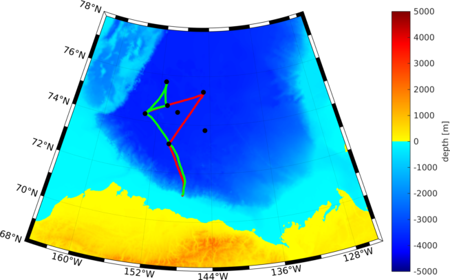
As part of the Canada Basin Glider Experiment (CABAGE), two Seagliders, SG196 and SG198, were deployed on 6 August 2017 at the shelf break north of Prudhoe Bay, AK. From there, they flew up to and around the CANAPE mooring array until they were recovered on 17 September 2017, for a total of 49 days. Together the gliders covered approximately 1730 km over the course of 712 dives, with SG196 diving to 480 m depth and SG198 diving to 750 m. Figure 2 shows the glider tracklines for both a short test deployment in 2016 and the 2017 deployment.

Figure 2: SG196 (green) and SG198 (red) were deployed at the shelf break north of Prudhoe Bay, AK. From there, they flew up to and around the CANAPE mooring array (black dots) for 49 days until they were recovered by the USCGC Healy.

Each glider was equipped with a Nortek Signature1000 1 MHz ADCP, as well as the standard suite of conductivity temperature (CT) sensor, pressure sensor, WHOI MicroModem, and custom-built passive marine acoustic recorders (PMARs). Figure 1 shows the gliders loaded on the R/V Ukpik, ready for launch, with the upward-facing ADCPs, installed in the tail section, clearly visible.

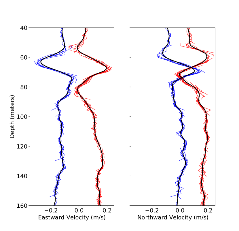
For clarity during the discussion here, when referring to the ADCP data, we will use trace to refer to an individual profile collected by the ADCP, and profile to refer to the result of the inverse, i.e. the current profile for the entire dive. The ADCPs were programmed to collect a trace every 15 seconds with 2.0 m bins. Each trace typically covered 10-15 m depth, with the actual usable range varying with the amount of acoustic scatterers in the water. In practice any given depth bin was covered by 5-7 different traces. Figure 3 illustrates a section of the current profile with overlapping ADCP traces after alignment.

VI Results

In this section we compare the results obtained using the approaches detailed in Sections III and IV.

Figure 3 shows a short section of the current profile with the individual overlapping traces that have been aligned and averaged to produce the final current profile (black). This is from a 750 m dive, so the sections of data shown were collected 3.5 hrs apart. The difference in the current profile during ascent and descent are clearly visible.

Figure 3: Overlapping ADCP traces during descent (blue) and ascent (red) for dive 99 of sg198, after alignment. The current profile produced by the state-space approach is shown as the thick black line.

Figure 4: Comparison of the full results from the method of Section III (black dashed) to that of Section IV (colored).

Figure 5: Zooming in on the upper 100m of the profiles in Figure 4, we use current profile data from a 600 kHz ADCP on a mooring that was approx. 13 km away during this dive. Current data was collected hourly. The time evolution of the surface currents over the 5 hours during the dive, is captured by the color scale, starting with blue at the beginning of the dive and ending with red.

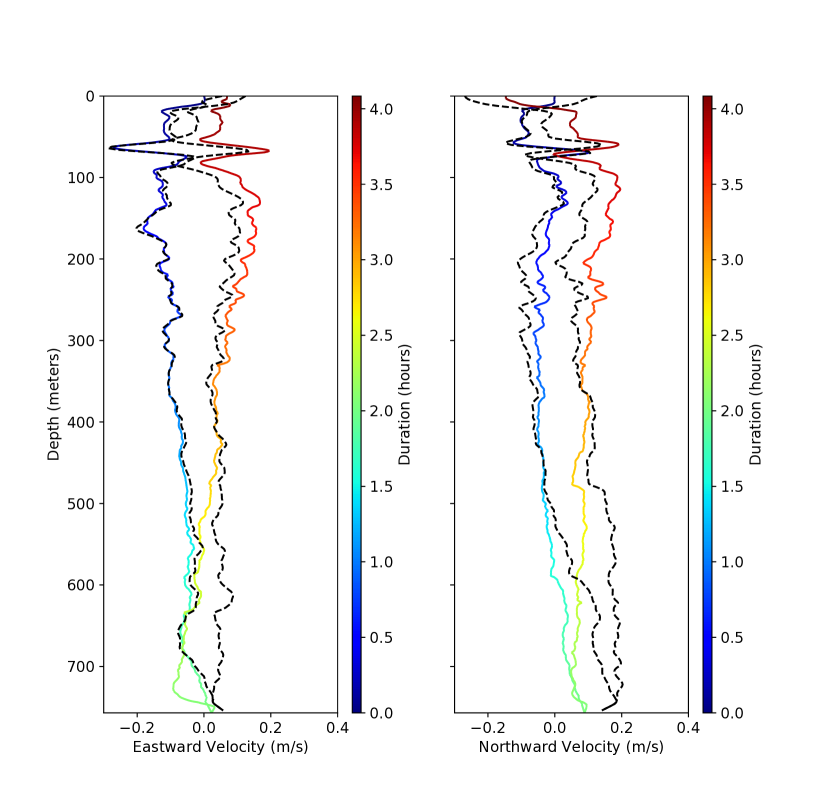
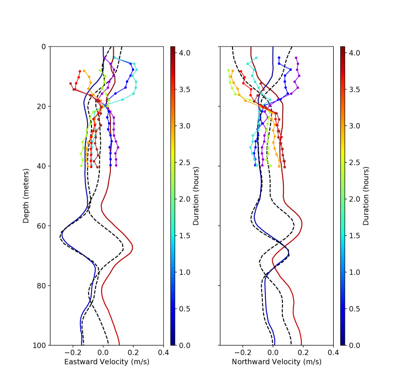
A comparison of the results of the two methods for the entire dive is shown in Figure 4. Both approaches find highly correlated estimates of current profiles, which is reassuring, though there is a clear offset between the results that varies by depth. We believe that this is due in large part to the sensitivity of the state-space approach to the weighting applied to the different terms in the minimization, which are difficult challenging to vet without ground truth for the entire current profile.

The only ground truth available for this dive is for the upper 40 m, shown in Figure 5. These data are from an upward-facing 600 kHz moored ADCP that was approximately 13 km away during this dive. The time evolution of the surface currents, measured hourly, is captured by the same color scale used for the glider data, starting with blue at the beginning of the dive and ending with red. Current data, as shown here, has not yet been corrected for the motion of the mooring. This correction and aggregate comparisons for other dives that are near moorings is the topic of future work.

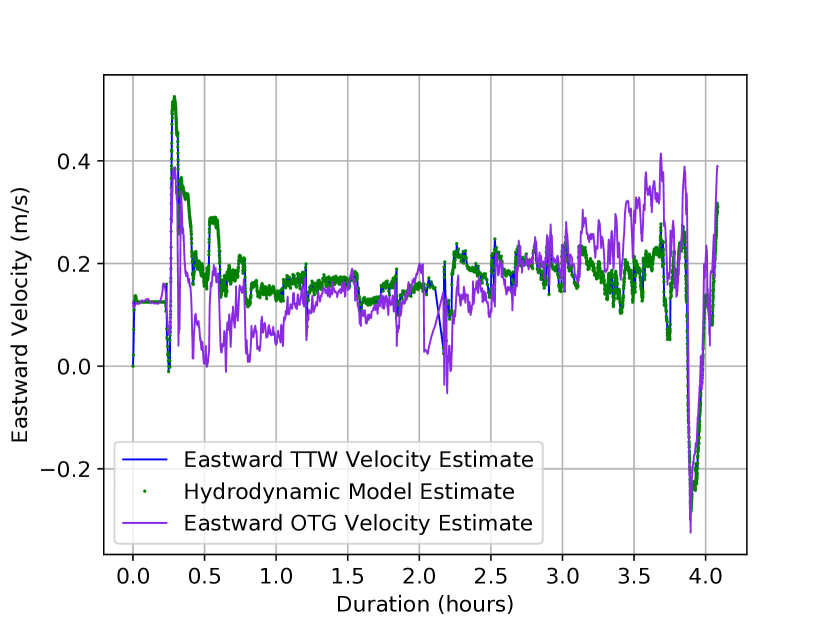
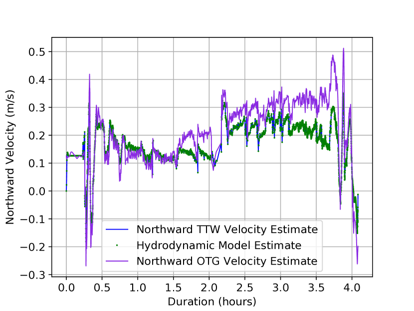
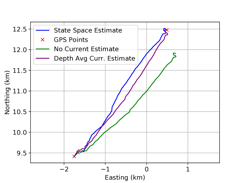
The second approach also produces updated velocity profiles, which are shown in Figure 6 and the resulting glider trajectory, shown in Figure 7. Comparing the x-y position estimates from a glider trajectory computed using the naive approach of uniformly applying a single depth-averaged current estimate across the dive versus using the ADCP-based current profile to inform the glider position throughout the dive, shows a dramatic difference. The ADCP-based correction not only shifts the trajectory, but also compresses the dive and stretches the climb. This leads to a maximum horizontal offset of 449m in this case. We look forward to using range measurements from the CANAPE moorings to both improve and validate these results in future work.

Figure 6: Updated velocities after processing the ADCP data.

Figure 7: We compare position estimates from a glider trajectory computed without knowledge of current (dead reckoning), using the naive approach of applying a depth-averaged current uniformly across the dive, and using the ADCP-based current profile to inform the glider position throughout the dive. The ADCP-based correction not only shifts the trajectory, but also compresses the dive and stretches the climb, leading to a max horizontal offset of 449m.

VII Conclusions and Future Work

The main contribution of the work is to validate the idea of solving the state-space and current deconvolution problem using ADCP measurements. Two related approaches were developed, implemented, and compared; both made use of glider-estimated velocities, ADCP observations, and GPS fixes. The estimated current profiles were reasonably comparable to those obtained by a ‘ground truth’ ADCP on a nearby mooring.

The state-space approach in Section IV is more informative than the first, since it also produces modified post-processed state estimates of the glider, see Figure 6. While there is no ground truth on the estimated velocities, the high degree of correlation between the deconvolution and inversion method for estimating current profiles validates the approach, and opens doors for future work using the state-space approach.

First, the state-space approach builds an explicit connection between variables used during navigation to those informed by the ADCP. This is a promising development for ADCP-aided navigation.

Second, the state-space framework allows a broad set of optimization-based tools to be applied to the deconvolution problem. In particular we can incorporate constraints [13], robust losses [14], and nonsmooth regularization [15, 16], as well as singular state-space models that make use of these innovations [17]. The state-space formulation also allows nonlinear models [13, 18], as needed by range measurements. All of these innovations make it possible to fuse information from noisy measurements along with statistical models that are robust to noisy data and constraints that incorporate prior knowledge. Efficient implementation of these formulations requires significant additional work in understanding the structure of the underlying linear algebra problem (3).

References

- [1] D. R. Yoerger, A. M. Bradley, B. B. Walden, H. Singh, and R. Bachmeyer, “Surveying a subsea lava flow using the autonomous benthic explorer (abe),” International Journal of Systems Science, vol. 29, no. 10, pp. 1031–1044, 1998.
- [2] C. J. McFarland, M. V. Jakuba, S. Suman, J. C. Kinsey, and L. L. Whitcomb, “Toward ice-relative navigation of underwater robotic vehicles under moving sea ice: Experimental evaluation in the arctic sea,” in Proc. IEEE Intl. Conf. Robot. Auto. (ICRA), May 2015, pp. 1527–1534.
- [3] E. Firing and R. L. Gordon, “Deep ocean acoustic Doppler current profiling,” in Proceedings of the IEEE Fourth Working Conference on Current Measurement, April 1990, pp. 192–201.
- [4] J. Fischer and M. Visbeck, “Deep velocity profiling with self-contained ADCPs,” Journal of Atmospheric and Oceanic Technology, vol. 10, no. 5, pp. 764–773, 1993.
- [5] M. Visbeck, “Deep velocity profiling using lowered acoustic Doppler current profilers: Bottom track and inverse solutions,” Journal of Atmospheric and Oceanic Technology, vol. 19, no. 5, pp. 794–807, 2002.
- [6] M. Stanway, “Water profile navigation with an acoustic doppler current profiler,” in Proc. IEEE/MTS OCEANS Conf. Exhib., Sydney, Australia, May 2010, pp. 1–5.
- [7] M. J. Stanway, “Dead reckoning through the water column with an acoustic doppler current profiler: Field experiences,” in Proc. IEEE/MTS OCEANS Conf. Exhib., Kona, HI, Sep. 2011, pp. 1–8.
- [8] L. Medagoda, M. V. Jakuba, O. Pizarro, and S. B. Williams, “Water column current profile aided localisation for autonomous underwater vehicles,” in Proc. IEEE/MTS OCEANS Conf. Exhib., Sydney, Australia, May 2010, p. 10 pp.
- [9] A. M. Thurnherr, D. Symonds, and L. St. Laurent, “Processing explorer ADCP data collected on Slocum gliders using the LADCP shear method,” in 2015 IEEE/OES Eleveth Current, Waves and Turbulence Measurement (CWTM), March 2015, pp. 1–7.
- [10] R. E. Todd, D. L. Rudnick, M. R. Mazloff, R. E. Davis, and B. D. Cornuelle, “Poleward flows in the southern California Current system: Glider observations and numerical simulation,” Journal of Geophysical Research: Oceans, vol. 116, no. C02026, pp. 2156–2202, 2011.
- [11] R. E. Todd, D. L. Rudnick, J. Sherman, W. Owens, and L. George, “Absolute velocity estimates from autonomous underwater gliders equipped with doppler current profilers,” J. Atmos. Oceanic Tech., vol. 34, no. 2, pp. 309–333, 2017.
- [12] R. E. Davis, “On the coastal-upwelling overturning cell,” J. Marine Res., vol. 68, no. 3-4, pp. 369–385, May 2010.
- [13] B. M. Bell, J. V. Burke, and G. Pillonetto, “An inequality constrained nonlinear Kalman–Bucy smoother by interior point likelihood maximization,” Automatica, vol. 45, no. 1, pp. 25–33, 2009.
- [14] A. Aravkin, J. Burke, and G. Pillonetto, “Robust and trend-following student’s t Kalman smoothers,” SIAM Journal on Control and Optimization, vol. 52, no. 5, pp. 2891–2916, 2014.
- [15] A. Y. Aravkin, J. V. Burke, and G. Pillonetto, “Sparse/robust estimation and Kalman smoothing with nonsmooth log-concave densities: Modeling, computation, and theory,” J. Mach. Learn. Res., vol. 14, no. 1, pp. 2689–2728, 2013.
- [16] A. Aravkin, J. V. Burke, L. Ljung, A. Lozano, and G. Pillonetto, “Generalized Kalman smoothing: Modeling and algorithms,” Automatica, vol. 86, pp. 63–86, 2017.
- [17] J. Jonker, A. Aravkin, J. V. Burke, G. Pillonetto, and S. Webster, “Fast robust methods for singular state-space models,” Automatica, vol. 105, pp. 399–405, 2019.
- [18] A. Y. Aravkin, J. V. Burke, and G. Pillonetto, “Optimization viewpoint on kalman smoothing with applications to robust and sparse estimation,” in Compressed sensing & sparse filtering. Springer, 2014, pp. 237–280.