Abstract

I argue that regularizing terms in standard regression methods not only help against overfitting finite data, but sometimes also yield better causal models in the infinite sample regime. I first consider a multi-dimensional variable linearly influencing a target variable with some multi-dimensional unobserved common cause, where the confounding effect can be decreased by keeping the penalizing term in Ridge and Lasso regression even in the population limit. Choosing the size of the penalizing term, is however challenging, because cross validation is pointless. Here it is done by first estimating the strength of confounding via a method proposed earlier, which yielded some reasonable results for simulated and real data.

Further, I prove a ‘causal generalization bound’ which states (subject to a particular model of confounding) that the error made by interpreting any non-linear regression as causal model can be bounded from above whenever functions are taken from a not too rich class. In other words, the bound guarantees ‘generalization’ from observational to interventional distributions, which is usually not subject of statistical learning theory (and is only possible due to the underlying symmetries of the confounder model).

1 Introduction

Predicting a scalar target variable $Y$ from a $d$-dimensional predictor ${\bf X}:=(X_{1},\dots,X_{d})$ via appropriate regression models is among the classical problems of machine learning, see e.g. Schölkopf & Smola (2002). In the standard supervised learning scenario, some finite number of observations, independently drawn from an unknown but fixed joint distribution $P_{Y,{\bf X}}$, are used for inferring $Y$-values corresponding to unlabelled ${\bf X}$-values. To solve this task, regularization is known to be crucial for obtaining regression models that generalize well from training to test data Vapnik (1998). Deciding whether such a regression model admits a causal interpretation is, however, challenging. Even if causal influence from $Y$ to ${\bf X}$ can be excluded (e.g. by time order), the statistical relation between ${\bf X}$ and $Y$ cannot necessarily be attributed to the influence of ${\bf X}$ on $Y$. Instead, it could be due to possible common causes, also called ‘confounders’. For the case where common causes are known and observed, there is a huge number of techniques to infer the causal influence, e.g., (Rubin, 2004), addressing different challenges, for instance, high dimensional confounders (Chernozhukov et al., 2018) or the case where some variables other than the common causes are observed (Pearl, 2000), just to mention a few of them. If common causes are not known, the task of inferring the influence of ${\bf X}$ on $Y$ gets incredibly hard. Given observations from any further variables other than ${\bf X}$ and $Y$, conditional independences may help to detect or disprove the existence of common causes (Pearl, 2000), and so-called instrumental variables may admit the identification of causal influence (Imbens & Angrist, 1994).

Here we consider the case where only observations from ${\bf X}$ and $Y$ are given. In this case, naively interpreting the regression model as causal model is a natural baseline. Within our simplified scenario, we show that strong regularization increases the chances that the regression model contains some causal truth. I am aware of the risk that this result could be mistaken as a justification to ignore the hardness of the problem and blindly infer causal models by strong regularization. My goal is, instead, to inspire a discussion on to what extent causal modelling should regularize even in the infinite sample limit due to some analogies between generalizing across samples from the same distribution and ‘generalizing’ from observational to interventional distributions, which appear in a particular model of confounding, while they need not apply to other confounding scenarios. The idea that regularization can also help for better generalization across different environments rather than only across different subsamples from the same distribution can already be found in the literature Heinze-Deml & Meinshausen (2017), but here I describe a model of confounding for which the analogy between confounding and overfitting is so tight that exactly the same techniques help against both.

Scenario 1: inferring a linear statistical model

To explain the idea, we consider the simple case where the statistical relation between ${\bf X}$ and $Y$ is given by the linear model

$$Y={\bf X}{\bf a}+E,$$ (1)

where ${\bf a}$ is a column vector in ${\mathbb{R}}^{d}$ and $E$ is an uncorrelated unobserved noise variable, i.e., $\Sigma_{{\bf X}E}=0$. We are given observations from ${\bf X}$ and $Y$. Let $\hat{Y}$ denote the column vector of centred renormalized observations $y^{i}$ of $Y$, i.e., with entries $(y^{i}-\frac{1}{n}\sum_{i=1}^{n}y^{i})/\sqrt{n-1}$, and similarly, $\hat{E}$ denotes the centred renormalized values of $E$. Likewise, let $\hat{{\bf X}}$ denote the $n\times d$ matrix whose $j$th column contains the centred renormalized observations from $X_{j}$. Let, further, $\hat{{\bf X}}^{-1}$ denote its (Moore-Penrose) pseudoinverse. To avoid overfitting, the least squares estimator

$$\hat{{\bf a}}:={\rm argmin}_{\bf a}^{\prime}\|\hat{Y}-\hat{{\bf X}}{\bf a}^{\prime}\|^{2}=\hat{{\bf X}}^{-1}\hat{Y}={\bf a}+\hat{{\bf X}}^{-1}\hat{E},$$ (2)

is replaced with the Ridge and Lasso estimators

$$\hat{{\bf a}}^{\rm ridge}_{\lambda} := {\rm argmin}_{{\bf a}^{\prime}}\{\lambda\|{\bf a}^{\prime}\|^{2}_{2}+\|\hat{Y}-\hat{{\bf X}}{\bf a}^{\prime}\|^{2}\}$$ (3)

$$\hat{{\bf a}}^{\rm lasso}_{\lambda} := {\rm argmin}_{{\bf a}^{\prime}}\{\lambda\|{\bf a}^{\prime}\|_{1}+\|\hat{Y}-\hat{{\bf X}}{\bf a}^{\prime}\|^{2}\},$$ (4)

where $\lambda$ is a regularization parameter (Hastie et al., 2001).

So far we have only described the standard scenario of inferring properties of the conditional $P_{Y|X}$ from finite observations $\hat{{\bf X}},\hat{Y}$ without any causal semantics.

Scenario 2: inferring a linear causal model

We now modify the scenario in three respects. First, we assume that $E$ and ${\bf X}$ in (1) correlate due to some unobserved common cause. Second, we interpret (1) in a causal way in the sense that setting ${\bf X}$ to ${\bf x}$ lets $Y$ being distributed according to ${\bf x}{\bf a}+E$. Using Pearl’s do-notation (Pearl, 2000), this can be phrased as

$$Y|_{do({\bf X}={\bf x})}={\bf x}{\bf a}+E\quad\neq Y|_{{\bf X}={\bf x}}.$$ (5)

Third, we assume the infinite sample limit where $P_{{\bf X},Y}$ is known. We still want to infer ${\bf a}$ because we are interested in causal statements but regressing $Y$ on ${\bf X}$ yields $\hat{{\bf a}}$ instead which describes the observational conditional on the right hand side of (5).

Conceptually, Scenario 1 and 2 deal with two entirely different problems: inferring $P_{Y|{X=x}}$ from finite samples $(\hat{{\bf X}},\hat{Y})$ versus inferring the interventional conditional $P_{Y|do({\bf X}={\bf x})}$ from the observational distribution $P_{Y,{\bf X}}$. However, in our case, both problems amount to inferring the vector ${\bf a}$. Further, for both scenarios, the error term $\hat{{\bf X}}^{-1}\hat{E}$ is responsible for the failure of ordinary least squares regression. Only the reason why this term is non-zero differs: in the first scenario it is a finite sample effect, while it results from confounding in the second one. The idea of the present paper is simply that standard regularization techniques do not care about the origin of this error term. Therefore, they can temper the impact of confounding in the same way as they help avoiding to overfit finite data. Such a strong statement, for course, relies heavily on our highly idealized generating model for the confounding term. We therefore ask the reader not to quote it without also mentioning the strong assumptions.

The paper is structured as follows. Section 2 elaborates on the analogy between overfitting and confounding by only slightly generalizing observations of Janzing & Schölkopf (2018). Section 3 describes population versions of Ridge and Lasso regression and provides a Bayesian justification. Section 4 proposes a way to determine the regularization parameter in scenario 2 by estimating the strength of confounding via a method proposed by Janzing & Schölkopf (2018). Section 5 describes some empirical results. Section 6 describes a modified statistical learning theory that states that regression models from not too rich function classes ‘generalize’ from statistical to causal statements.

2 Analogy between overfitting and confounding

The reason why our scenario 2 only considers the infinite sample limit of confounding is that mixing finite sample and confounding significantly complicates the theoretical results. For a concise description of the population case, we consider the Hilbert space ${\cal H}$ of centred random variables (on some probability space without further specification) with finite variance. The inner product is given by the covariance, e.g.,

$$\langle X_{i},X_{j}\rangle:={\rm cov}(X_{i},X_{j}).$$ (6)

Accordingly, we can interpret ${\bf X}$ as an operator ${\mathbb{R}}^{d}\to{\cal H}$ via $(b_{1},\dots,b_{d})\mapsto\sum_{j}b_{j}X_{j}$. Then the population version of (2) reads

$$\tilde{{\bf a}}={\rm argmin}_{\bf a}^{\prime}\{\|Y-{\bf X}{\bf a}^{\prime}\|^{2}\}={\bf X}^{-1}Y={\bf a}+{\bf X}^{-1}E,$$ (7)

where the square length is induced by the inner product (6), i.e., it is simply the variance. Extending the previous notation, ${\bf X}^{-1}$ now denotes the pseudoinverse of the operator ${\bf X}$ (Beutler, 1965). To see that ${\bf X}^{-1}E$ is only non-zero when ${\bf X}$ and $E$ are correlated it is helpful to rewrite it as

$${\bf X}^{-1}E=\Sigma_{{\bf X}{\bf X}}^{-1}\Sigma_{{\bf X}E},$$ (8)

where we have assumed $\Sigma_{{\bf X}{\bf X}}$ to be invertible (see appendix for a proof). The claim that standard regularization like Ridge and Lasso work for tempering the impact of the term ${\bf X}^{-1}E$ in the same way as they work for $\hat{{\bf X}}^{-1}\hat{E}$ is inspired by the observation of Janzing & Schölkopf (2018) that these terms follow the same distribution subject to the idealized model assumptions described there. We obtain the same analogy for a slightly more general model which we describe now.

Figure 1: Left: In scenario 1, the empirical correlations between $X$ and $E$ are only finite sample effects. Right: In scenario 2, ${\bf X}$ and $E$ are correlated due to their common cause ${\bf Z}$. We sample the structural parameters $M$ and ${\bf c}$ from distributions in a way that entails a simple analogy between scenario 1 and 2.

Generating model for scenario 1

The following procedure generates samples according to the DAG in Figure 1, left:

1.	Draw $n$ observations from $(X_{1},\dots,X_{d})$
	independently from $P_{X}$
2.	Draw samples of $E$ independently from $P_{E}$
3.	Draw the vector ${\bf a}$ of structure coefficients
	from some distribution $P_{\bf a}$
4.	Set $\hat{Y}:=\hat{{\bf X}}{\bf a}+\hat{E}$.

Generating model for scenario 2

To generate random variables according to the DAG in Figure 1, right, we assume that both variables ${\bf X}$ and $E$ are generated from the same set of independent sources by applying a random mixing matrix or a random mixing vector, respectively:

Given an $\ell$-dimensional random vector ${\bf Z}$ of sources with distribution ${\cal N}(0,I)$.

1 .	Choose an $\ell\times d$ mixing matrix $M$
	and set ${\bf X}:={\bf Z}M$.
2.	Draw ${\bf c}\in{\mathbb{R}}^{\ell}$ from some distribution $P_{\bf c}$
	and set $E:={\bf Z}{\bf c}.$
3.	Draw the vector ${\bf a}$ of structure coefficients
	from some distribution $P_{\bf a}$
4.	Set $Y:={\bf X}{\bf a}+E$.

We then obtain:

Theorem 1 (population and empirical covariances).

Let the number $\ell$ of sources in scenario 2 be equal to the number $n$ of samples in scenario 1 and $P_{M}$ coincide with the distribution of sample matrices $\hat{{\bf X}}$ induced by $P_{\bf X}$. Let, moreover, $P_{\bf c}$ in scenario 2 coincide with the distribution of $\hat{E}$ induced by $P_{E}$ in scenario 1, and $P_{\bf a}$ be the same in both scenarios. Then the joint distribution of ${\bf a},\Sigma_{{\bf X}{\bf X}},\Sigma_{{\bf X}Y},\Sigma_{{\bf X}E}$ in scenario 2 coincides with the joint distribution of ${\bf a},\widehat{\Sigma_{{\bf X}{\bf X}}},\widehat{\Sigma_{{\bf X}Y}},\widehat{\Sigma_{{\bf X}E}}$ in scenario 1.

Proof.

We have $\widehat{\Sigma_{{\bf X}{\bf X}}}=\hat{{\bf X}}^{T}\hat{{\bf X}}$ and $\Sigma_{{\bf X}{\bf X}}={\bf X}^{T}{\bf X}=M^{T}{\bf Z}^{T}{\bf Z}M=M^{T}M$, where we have used that ${\bf Z}$ has full rank due to the uncorrelatedness of its components. Likewise, $\widehat{\Sigma_{{\bf X}E}}=\hat{{\bf X}}^{T}\hat{E}$ and $\Sigma_{{\bf X}E}=({\bf Z}M)^{T}{\bf Z}{\bf c}=M^{T}{\bf c}$. Further, $\widehat{\Sigma_{{\bf X}Y}}=\hat{{\bf X}}^{T}{\bf X}{\bf a}+\hat{\Sigma_{{\bf X}E}}$ and $\Sigma_{{\bf X}Y}={\bf X}^{T}{\bf X}{\bf a}+\Sigma_{{\bf X}E}$. Then the statement follows from the correspondences $M\equiv\hat{{\bf X}}$, ${\bf c}\equiv\hat{E}$, ${\bf a}\equiv{\bf a}$. ∎

Theorem 1 provides a canonical way to transfer methods for inferring the vector ${\bf a}$ from empirical covariance matrices in scenario 1 to similar methods for inferring ${\bf a}$ in scenario 2 from population covariance matrices. Motivated by this insight we will now develop our ‘causal’ Ridge and Lasso for the population case. To emphasize that this method uses weaker assumptions than Theorem 1, we will not strictly build on it and use a more abstract condition that is only motivated by the concrete model above.

3 Bayesian justification for Ridge and Lasso in scenario 2

We now define population versions of Ridge and Lasso that temper confounding in the same way as the usual versions temper overfitting.

$$\tilde{{\bf a}}^{\rm ridge}_{\lambda} := {\rm argmin}_{{\bf a}^{\prime}}\{\lambda\|{\bf a}^{\prime}\|^{2}_{2}+\|Y-{\bf X}{\bf a}^{\prime}\|^{2}\}$$ (9)

$$\tilde{{\bf a}}^{\rm lasso}_{\lambda} := {\rm argmin}_{{\bf a}^{\prime}}\{\lambda\|{\bf a}^{\prime}\|_{1}+\|Y-{\bf X}{\bf a}^{\prime}\|^{2}\}.$$ (10)

We briefly sketch standard Bayesian arguments for the finite sample versions Hoerl & Kennard (2000). Let the prior distributions for ${\bf a}$ be given by

$$p_{\rm ridge}({\bf a}) \sim \exp\left(-\frac{1}{2\tau^{2}}\|{\bf a}\|^{2}\right)$$ (11)

$$p_{\rm lasso}({\bf a}) \sim \exp\left(-\frac{1}{2\tau^{2}}\|{\bf a}\|_{1}\right).$$ (12)

If we assume that the noise variable $E$ is Gaussian with standard deviation $\sigma_{E}$ we obtain

$$p({\bf y}|{\bf x},{\bf a})\sim\exp\left(-\frac{1}{2\sigma_{E}^{2}}\|{\bf y}-{\bf x}{\bf a}\|^{2}\right),$$

which yields the posteriors

$$\log p_{\rm ridge}({\bf a}|\hat{{\bf X}},\hat{Y}) \stackrel{{\scriptstyle+}}{{=}}-\frac{1}{2\tau^{2}}\|{\bf a}\|^{2}-\frac{1}{2\sigma_{E}^{2}}\|\hat{Y}-\hat{{\bf X}}{\bf a}\|^{2}$$ (13)

$$\log p_{\rm lasso}({\bf a}|\hat{{\bf X}},\hat{{\bf Y}}) \stackrel{{\scriptstyle+}}{{=}}-\frac{1}{2\tau^{2}}\|{\bf a}\|_{1}-\frac{1}{2\sigma_{E}^{2}}\|\hat{Y}-\hat{{\bf X}}{\bf a}\|^{2},$$ (14)

which are maximized for $\hat{{\bf a}}_{\lambda}$ in (3) and (4), respectively, after setting $\lambda=\sigma^{2}_{E}/\tau^{2}$ (here $\stackrel{{\scriptstyle+}}{{=}}$ denotes equality up to an additive ${\bf a}$-independent term).

To derive the posterior for ${\bf a}$ for scenario 2, we recall that now the entire distribution $P_{{\bf X},Y}$ is given. We also know that ${\bf X}$ ad $Y$ are related by $Y={\bf X}{\bf a}+E$, but ${\bf a}$ and $E$ are unknown. For ${\bf a}$ we will adopt the priors (11) and (12), but to define a reasonable prior for $E$ is less obvious. Note that we are not talking about a prior for the values attained by $E$. Instead, $E$ is an unknown vector in the infinite dimensional Hilbert space ${\cal H}$. Fortunately, we do not need to specify a prior for $E$, it is sufficient to specify a prior for the projection $E_{\bf X}$ onto the image of ${\bf X}$. We assume:

$$E_{\bf X}\sim{\cal N}(0,\sigma_{E_{\bf X}}^{2}{\bf I})$$ (15)

for some ‘confounding parameter’ $\sigma_{E_{\bf X}}^{2}$. This implies the following distribution for the projection $Y_{\bf X}$ of $Y$ onto the image of ${\bf X}$:

$$p(Y_{\bf X}|{\bf X},{\bf a})\sim\exp\left(-\frac{1}{\sigma_{E_{\bf X}}^{2}}\|Y_{\bf X}-{\bf X}{\bf a}\|^{2}\right).$$

This way, we obtain the following posteriors for ${\bf a}$:

$$\log p_{\rm ridge}({\bf a}|{\bf X},Y_{\bf X}) \stackrel{{\scriptstyle+}}{{=}}-\frac{1}{2\tau^{2}}\|{\bf a}\|^{2}-\frac{1}{2\sigma_{E_{\bf X}}^{2}}\|Y_{\bf X}-{\bf X}{\bf a}\|^{2}$$ (16)

$$\log p_{\rm lasso}({\bf a}|{\bf X},Y_{\bf X}) \stackrel{{\scriptstyle+}}{{=}}-\frac{1}{2\tau^{2}}\|{\bf a}\|_{1}-\frac{1}{2\sigma_{E_{\bf X}}^{2}}\|Y_{\bf X}-{\bf X}{\bf a}\|^{2}.$$ (17)

After replacing $Y_{\bf X}$ with $Y$ (which is irrelevant for the maximization) we observe that the posterior probabilities are maximized by (9) and (10) with $\lambda:=\sigma_{E_{\bf X}}^{2}/\tau^{2}$.

We phrase our findings as a theorem:

Theorem 2 (justification of population Ridge and Lasso).

Given a $d$-dimensional random variable ${\bf X}$ and a scalar random variable $Y$ for which $P_{{\bf X},Y}$ is known. Let they be linked by

$$Y={\bf X}{\bf a}+E,$$

where ${\bf a}\in{\mathbb{R}}^{d}$ is unknown and $E$ is a random variable whose distribution is unknown. Assume (11) and (12) as priors for ${\bf a}$, respectively. Assume that the projection $E_{\bf X}$ of $E$ on the image of ${\bf X}$ follows the prior distribution

$$E_{\bf X}\sim\exp\left(-\frac{1}{2\sigma_{E_{\bf X}}^{2}}\|E_{\bf X}\|^{2}\right).$$

Then the posterior probability $p({\bf a}|P_{{\bf X},Y})$ is maximized by the population Ridge and Lasso estimators (9) and (10), respectively, for $\lambda:=\sigma_{E_{\bf X}}^{2}/\tau^{2}$.

Here we decided to write $p({\bf a}|P_{{\bf X},Y})$ instead of $p({\bf a}|{\bf X},Y)$ to avoid that it could be misunderstood as the conditional given observations from ${\bf X},Y$ instead of the entire statistics. In the derivations above it was convenient to keep them as similar to the finite sample case as possible by simply removing the symbol $\hat{}$.

The results raise the questions how to select $\lambda$ for our population Ridge and Lasso. First note that information criteria like AIC and BIC (Chakrabarti & Ghosh, 2011) cannot be applied: since they require the sample size in scenario 1, they would require the number of sources in scenario 2, which we assume to be unknown (assuming it to be known seems to go too far away from real-world scenarios). To focus on another standard approach of choosing $\lambda$, note that transferring cross-validation (Hastie et al., 2001) from scenario 1 to scenario 2 requires data from different distributions (recall that drawing $\hat{{\bf X}},\hat{E}$ corresponds to drawing $M$ and ${\bf c}$ in Section 2), which we do not assume to be available here. Therefore we need to estimate the strength of confounding to choose the regularization constant.

4 Choosing the regularization constant by estimating confounding

The only approaches that directly estimate the strength of confounding from $P_{{\bf X},Y}$ alone we are aware of are given by Janzing & Schölkopf (2017; 2018). The first paper considers only one-dimensional confounders, which is complementary to our confounding scenario, while we will use the approach from the second paper because it perfectly matches our scenario 2 in Section 2 with fixed $M$. Janzing & Schölkopf (2018) use the slightly stronger assumption that ${\bf a}$ and ${\bf c}$ are drawn from ${\cal N}(0,\sigma^{2}_{a}I)$ and ${\cal N}(0,\sigma^{2}_{c}I)$, respectively. We briefly rephrase the method.

The idea is that the unregularized regression vector $\tilde{{\bf a}}$ in (7) follows the distribution ${\cal N}(0,\sigma_{a}^{2}{\bf I}+\sigma_{c}^{2}M^{-1}M^{-T})$. This results from

$$\tilde{{\bf a}}={\bf a}+X^{-1}E={\bf a}+M^{-1}{\bf c},$$

(see proof of Theorem 1 by Janzing & Schölkopf (2018)). Then the quotient $\sigma_{c}^{2}/\sigma^{2}_{a}$ can be inferred from the direction of $\hat{{\bf a}}$ (intuitively: the more $\hat{{\bf a}}$ concentrates in small eigenvalue eigenspaces of $\Sigma_{{\bf X}{\bf X}}=M^{T}M$, the larger is this quotient). Using some approximations that hold for large $d$, the confounding strength

$$\beta:=\frac{\|\tilde{{\bf a}}-{\bf a}\|^{2}}{\|\tilde{{\bf a}}-{\bf a}\|^{2}+\|{\bf a}\|^{2}}\in[0,1]$$ (18)

can be estimated from the input $(\widehat{\Sigma_{{\bf X}{\bf X}}},{\bf a}^{\prime})$. Janzing & Schölkopf (2018) already observed the analogy between overfitting and confounding and also used the algorithm to estimate overfitting in scenario 1, which inspired this work. Using the approximation $\|\tilde{{\bf a}}-{\bf a}\|^{2}+\|{\bf a}\|^{2}\approx\|\tilde{{\bf a}}\|^{2}$ Janzing & Schölkopf (2017), we have $\|{\bf a}\|^{2}\approx(1-\beta)\cdot\|\tilde{{\bf a}}\|^{2}.$ Hence, the length of the true causal regression vector ${\bf a}$ can be estimated from the length $\tilde{{\bf a}}$. This way, we can adjust $\lambda$ such that $\|\hat{{\bf a}}_{\lambda}\|$ coincides with the estimated length. Since the estimation is based on a Gaussian (and not a Laplacian) prior for ${\bf a}$, it seems more appropriate to combine it with Ridge regression than with Lasso. However, since Lasso regression is known to have important advantages (e.g. that sparse solutions yield more interpretable results), we also use Lasso. After all, the qualitative statement that strong confounding amounts to vectors $\hat{{\bf a}}$ that tend to concentrate in low eigenvalue subspaces of $\Sigma_{{\bf X}{\bf X}}$ still hold true when ${\bf c}$ is chosen from an isotropic prior.

Confounding estimation via the algorithm of Janzing & Schölkopf (2018) requires the problematic decision of whether the variables $X_{j}$ should be rescaled to variance $1$. If different $X_{j}$ refer to different units, there is no other straightforward choice of the scale. It is not recommended, however, to always normalize $X_{j}$. If $\Sigma_{{\bf X}{\bf X}}$ is diagonal, for instance, the method would be entirely spoiled by normalization. The difficulty of deciding whether data should be renormalizing as an additional preprocessing step will be inherited by our algorithm.

Our confounder correction algorithm reads:

ConCorr

1:  Input: I.i.d. samples from $P({\bf X},Y)$.

2:  Rescale $X_{j}$ to variance $1$ if desired.

3:  Compute the empirical covariance matrices $\widehat{\Sigma_{{\bf X}{\bf X}}}$ and $\widehat{\Sigma_{{\bf X}Y}}$

4:  Compute the regression vector $\hat{{\bf a}}:=\widehat{\Sigma_{{\bf X}{\bf X}}}^{-1}\widehat{\Sigma_{{\bf X}Y}}$

5:  Compute an estimator $\hat{\beta}$ for the confounding strength $\beta$ via the algorithm in Janzing & Schölkopf (2018) from $\widehat{\Sigma_{{\bf X}{\bf X}}}$ and $\hat{{\bf a}}$ and estimate the squared length of ${\bf a}$ via

$$\|{\bf a}\|^{2}\approx(1-\hat{\beta})\|\hat{{\bf a}}\|^{2}$$ (19)

6:  find $\lambda$ such that the squared length of $\hat{{\bf a}}^{\tt lasso/ridge}_{\lambda}$ coincides with the right hand side of (19)

7:  Compute Ridge or Lasso regression model using this value of $\lambda$

8:  Output: Regularized regression vector ${\bf a}_{\lambda}$

5 Experiments

5.1 Simulated data

We have generated data in a way that admits moving between scenarios 1 and 2 by simply changing some parameters. For some fixed values of $d$ and $\ell$, we generate one mixing matrix $M$ in each run by drawing its entries from the standard normal distribution. In each run we generate $n$ instances of the $\ell$-dimensional standard normal random vector ${\bf Z}$ and compute the ${\bf X}$ values by ${\bf X}={\bf Z}M$. Then we choose $\sigma_{c}$, the parameter that crucially controls confounding: for $\sigma_{c}=0$, we obtain scenario 1. For scenario 2, we choose $\sigma_{c}$ uniformly at random from $[0,1]$. Likewise, we draw $\sigma_{a}$, the parameter that controls the strength of the causal influence, uniformly at random from $[0,1]$. Then we draw the entries of ${\bf c}$ and ${\bf a}$ from ${\cal N}(0,\sigma_{c}^{2})$ and ${\cal N}(0,\sigma^{2}_{a})$, respectively, and compute the values of $Y$ via $Y={\bf X}{\bf a}+{\bf Z}{\bf c}+E,$ where $E$ is random noise drawn from ${\cal N}(0,\sigma^{2}_{E})$ (the parameter $\sigma_{E}$ has previously been chosen uniformly at random from $[0,5]$, which yields quite noisy data). While such a noise term didn’t exist in our description of scenario 2, we add it here to study typical finite sample effects (without noise, $Y$ depends deterministically on ${\bf X}$ for $\ell\leq d$).

To evaluate the performance of causal regularization we define the relative squared error of any regression vector ${\bf a}^{\prime}$ by

$$\epsilon_{{\bf a}^{\prime}}:=\frac{\|{\bf a}^{\prime}-{\bf a}\|^{2}}{\|{\bf a}^{\prime}-{\bf a}\|^{2}+\|{\bf a}\|^{2}}.$$

Note that $\|{\bf a}^{\prime}-{\bf a}\|^{2}+\|{\bf a}\|^{2}\approx\|{\bf a}^{\prime}\|^{2}$ whenever the error $\|{\bf a}^{\prime}-{\bf a}\|^{2}$ is close to orthogonal to ${\bf a}$, which is a priori likely for vectors in high dimensions. Then $\epsilon_{{\bf a}^{\prime}}\approx\|{\bf a}^{\prime}-{\bf a}\|^{2}/\|{\bf a}^{\prime}\|^{2}$, which justifies the name ‘relative squared error’.

For the special case where ${\bf a}^{\prime}$ is the unregularized regression vector $\hat{{\bf a}}$ in (2), we define

$$\epsilon_{\rm unreg}:=\frac{\|\hat{{\bf a}}-{\bf a}\|^{2}}{\|\hat{{\bf a}}-{\bf a}\|^{2}+\|{\bf a}\|^{2}},$$

by slightly overloading notation. In the infinite sample limit $\epsilon_{\rm unreg}$ converges to the confounding strength $\beta$, see (18).

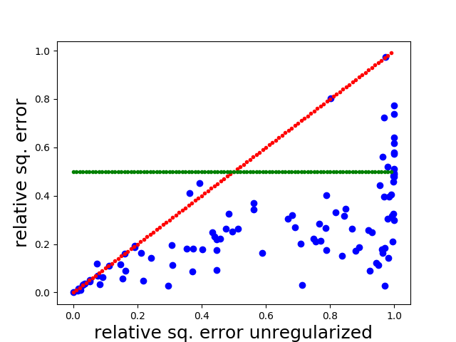
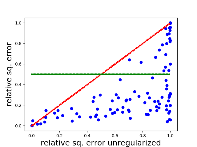
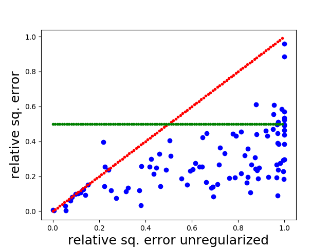
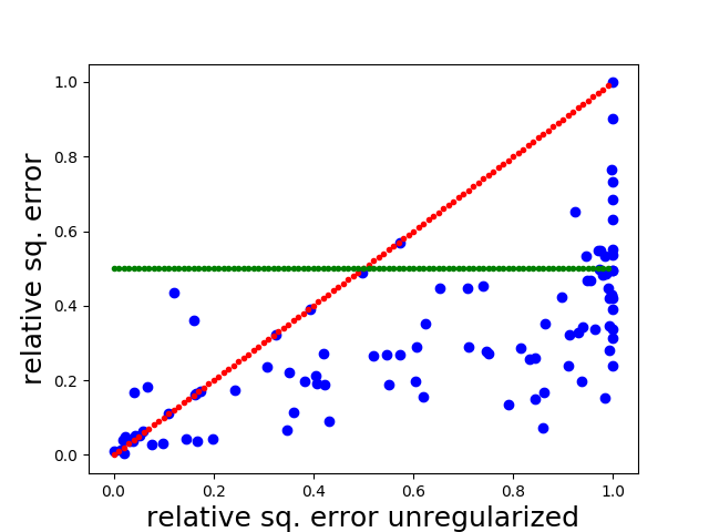
We begin with the unconfounded case $\sigma_{c}=0$ with $d=\ell=30$ and $n=50$. Figures 2, left and right, show the relative squared errors obtained by our method ConCorr over the unregularized errors. The red and green lines show two different baselines: first, the unregularized error, and second, the error $1/2$ obtained by the trivial regression vector $0$. The goal is to stay below both baselines. Apart from those two trivial baselines, another natural baseline is regularized regression where $\lambda$ is chosen by cross-validation, because this would be the default approach for the unconfounded case. We have used leave-one-out CV from the Python package scikit for Ridge and Lasso, respectively.

Figure 2: Results for Ridge (top) and Lasso (bottom) regression with ConCorr (left) versus cross-validated version (right) for the unconfounded case where artifacts are only due to overfitting. The results are roughly the same.

To quantitatively evaluate the performance, we have defined the success rate as the fraction of cases in which the relative squared error is at least by $0.05$ below both baselines, the unregularized relative squared error and the value $1/2$. Likewise, we define the failure rate as the fraction of cases where the relative squared error is by $0.05$ larger than at least one of the baselines. We obtained the following results:

method	successes	failures
ConCorr Ridge/Lasso	$0.63/0.61$	$0.11/0.16$
CV Ridge/Lasso	$0.65/0.72$	$0.21/0.15$

The results are roughly comparable, if we abstain from over-interpretations. In the regime where the unregularized relative squared error is around $1/2$, all $4$ methods yield errors that are most of the time significantly lower. All $4$ methods have problems in the regime where the unregularized error is close to $1$ and sometimes regularize to little for these cases.

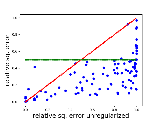
To test the performances for scenario 2, we considered the large sample case ($n=1000$, $d=30$) with confounding, where we obtained the results in Figure 3.

Figure 3: Results for Ridge (top) and Lasso (bottom) regression with ConCorr (left) versus cross-validated version (right) for the confounded case with large sample size where artifacts are almost only due to confounding.

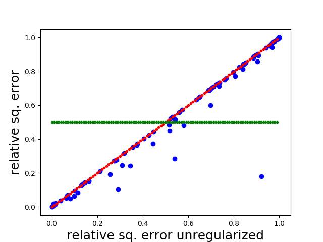
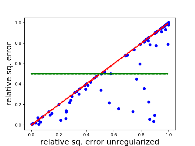
Remarkably, ConCorr performed quite quite well also with Lasso regression although the Laplacian prior of Lasso does not match our data generating process where the vector ${\bf a}$ has been chosen from a Gaussian. One may argue that experiments for the confounded large sample regime are pointless since our theory states the equivalence of scenario 1 and 2. We show the experiments nevertheless for two reasons. First, it is not obvious which sample size approximates the population limit sufficiently well, and second, we have, by purpose, not chosen the parameters for generating $M$ according to the theoretical correspondence in order not to repeat equivalent experiments. The success and failure rates read:

method	successes	failures
ConCorr Ridge/Lasso	$0.69/0.55$	$0.08/0.13$
CV Ridge/Lasso	$0.08/0.15$	$0.56/0.54$

Figure 4: Results for Ridge (left) and Lasso (right) regression for the data from the optical device in Janzing & Schölkopf (2018). The $y$-axis is the relative squared error achieved by ConCorr, while the $x$-axis is the cross-validated baseline.

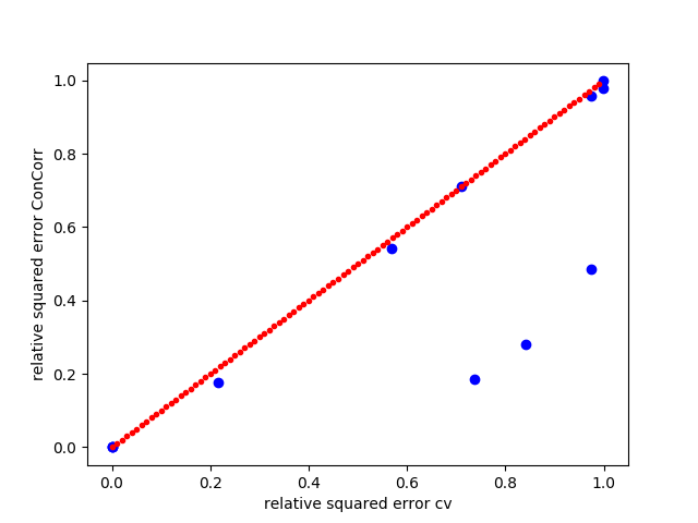
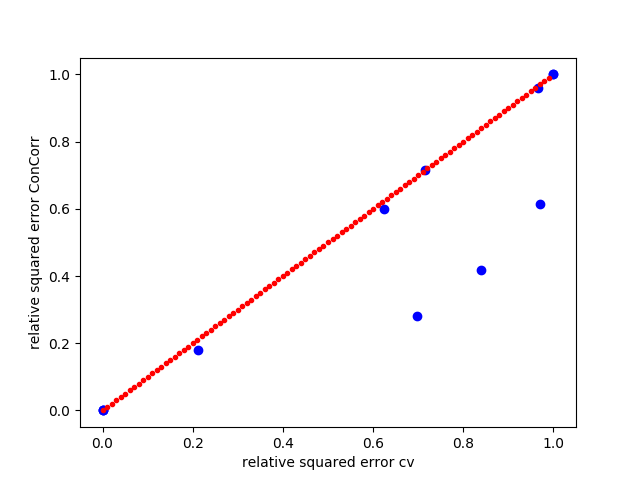
Here, ConCorr clearly outperforms cross-validation (for both Ridge and Lasso), which shows that cross-validation regularizes too weakly for causal modelling, as expected. One should add, however, that we increased the number of iterations in the $\lambda$-optimization to get closer to optimal leave-one-out performance since the default parameters of scikit already resulted in regularizing more strongly than that. Note that the goal of this paper is not to show that ConCorr outperforms other methods. Instead, we want to argue that for causal models it is often recommended to regularize more strongly than criteria of statistical predictability suggests. If ‘early stopping’ in common CV algorithms also yields stronger regularization, this can be equally helpful for causal inference, although the way ConCorr choses $\lambda$ is less arbitrary than just bounding the number of iterations.

We briefly mention results for the confounded case with small sample size, a regime for which we have no theoretical results. Here, CV Lasso performs comparably to ConCorr, which is probably due to the strong finite sample effects.

We also checked how the performance depends on the dimension, but one should not overestimate the value of these experiments since the estimation of confounding already depends heavily on the distribution of eigenvalues of $\Sigma_{{\bf X}{\bf X}}$.

5.2 Real data

To get confounded real data with ${\bf X}$ and $Y$ being linked by a linear causal relation with known regression vector is not easy. One approach is to restrict an unconfounded model to a subset of variables: whenever $Y={\bf X}{\bf a}+E$ is unconfounded, the statistical relation between $Y$ and a subset of ${\bf X}$ can become confounded by dropping parts of ${\bf X}$ that influence $Y$ (if the dropped components and the remaining ones have a common cause or the dropped ones influence the remaining ones). The true causal regression vector for the reduced system is given by simply reducing ${\bf a}$ to the respective components (if the sample size is large enough to avoid overfitting, which we assume below in agreement with Janzing & Schölkopf (2018)). However, to find multivariate data that is known to be unconfounded is difficult too.

Optical device

For this reason, (Janzing & Schölkopf, 2018) have build an optical device where the screen of a Laptop shows an image with extremely low resolution (in their case $3\times 3$-pixel) captured from a webcam. In front of the screen they mounted a photodiode measuring the light intensity $Y$, which is mainly influenced by the pixel vector ${\bf X}$ of the image.

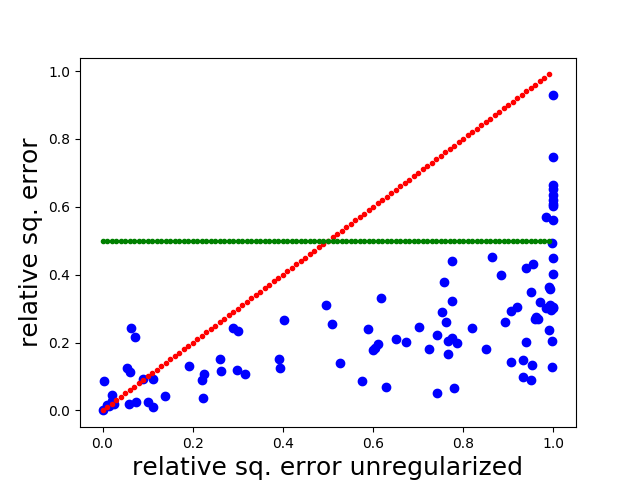
As confounder $W$ they generated a random voltage controlling two LEDs, one in front of the webcam (and thus influencing ${\bf X}$) and the second one in front of the photodiode (thus influencing $Y$). Since $W$ is also measured, the vector ${\bf a}_{{\bf X},W}$ obtained by regressing $Y$ on $({\bf X},W)$ is causal (no confounders by construction), if one accepts the linearity assumption. Dropping $W$ yielded significant confounding, with $\beta$ ranging from $0$ to $1$. We applied ConCorr to ${\bf X},Y$ and compared the output with the ground truth. Figure 4, left and right, show the results for Ridge and Lasso, respectively. The point $(0,0)$ happened to be met by three cases, where no improvement was possible. Fortunately, ConCorr did not make the result worse. One can see that in $3$ out of the remaining nine cases (note that the point $(1,1)$ is also met by two cases), ConCorr significantly improved the causal prediction. Fortunately, there is no case where ConCorr is worse than the baseline.

Taste of wine

(Janzing & Schölkopf, 2018), moreover, used a dataset from the UCI machine learning repository Newman et al. (1998) of which they believe that it is almost unconfounded. ${\bf X}$ contains $11$ ingredients of different sorts of red wine and $Y$ is the taste assigned by human subjects. Regressing $Y$ on ${\bf X}$ yields a regression vector for which the ingredient alcohol dominates. Since alcohol strongly correlates with some of the other ingredients, dropping it amounts to significant confounding (assuming that the correlations between alcohol and the other ingredients is due to common causes and not due to the influence of alcohol on the others).

After normalizing the ingredients, ConCorr with Ridge and Lasso yielded a relative error of $0.45$ and $0.35$, respectively, while Janzing & Schölkopf (2018) computed the confounding strength $\beta\approx 0.8$, which means that ConCorr significantly corrects for confounding (we confirmed that CV also yielded errors close to $0.8$ which suggests that finite sample effects did not matter for the error).

6 Learning theory on ‘generalization’ from observational to interventional distributions

So far, we have motivated causal regularization mainly via transferring Bayesian arguments for regularization from scenario 1 to scenario 2. An alternative perspective on regularization is provided by statistical learning theory (Vapnik, 1998). Generalization bounds guarantee that the expected error is unlikely to significantly exceed the empirical error for any regression function $f$ from a not too rich class ${\cal F}$. We will argue that our analogy between overfitting and confounding can be further extended to translate generalization bounds in a way that they bound the error made by the causal interpretation of regression models when they are taken from a not too rich model class. To make the analogy as natural as possible, we rephrase usual generalization bounds as:

error of $f$ w.r.t. true (observational) distribution

$\leq$ error of $f$ w.r.t. empirical distribution + $C({\cal F})$,

where $C({\cal F})$ is some ‘capacity’ term that accounts for the richness of the class ${\cal F}$. Then we expect, subject to some conditions on the confounder, ‘causal generalization bounds’ of the form :

error of $f$ w.r.t. interventional distribution

$\leq$ error of $f$ w.r.t. observational distribution + $C({\cal F})$.

Figure 5: Our confounding scenario: the high-dimensional common cause ${\bf Z}$ influences $Y$ in a linear additive way, while the influence on ${\bf X}$ is arbitrary.

Figure 5 shows our confounding model that significantly generalizes our previous models. ${\bf Z}$ and ${\bf X}$ are arbitrary random variables of dimensions $\ell$ and $d$, respectively. Apart from the graphical structure, we only add the parametric assumption that the influence of ${\bf Z}$ on ${\bf Y}$ is linear additive:

$$Y=Y^{\prime}+{\bf Z}{\bf c},$$ (20)

where ${\bf c}\in{\mathbb{R}}^{\ell}$. The change of $Y$ caused by setting ${\bf X}$ to ${\bf x}$ via interventions is given by Pearl’s backdoor criterion (Pearl, 2000) via

$$p(y|do({\bf x}))=\int p(y|{\bf x},{\bf z})p({\bf z})d{\bf z}.$$

For any function $f:{\mathbb{R}}^{d}\to{\mathbb{R}}$ we want to quantify how well it captures the behavior of $Y$ under interventions on ${\bf X}$ and introduce the interventional loss

$$\mathbf{E}_{do({\bf X})}[(Y-f({\bf X}))^{2}]:=\int(y-f({\bf x}))^{2}p(y|do({\bf x}))p({\bf x})d{\bf x}.$$ (21)

We want to compare it to the observational loss

$$\mathbf{E}[(Y-f({\bf X}))^{2}]=\int(y-f({\bf x}))^{2}p(y|{\bf x})p({\bf x})d{\bf x}.$$ (22)

In other words, we compare the expectations of the random variable $(Y-f({\bf X}))^{2}$ w.r.t.  the distributions $p(y,{\bf x})$ and $p(y|do({\bf x}))p({\bf x})$. The appendix shows that the difference between (21) and (22) can be concisely phrases in terms of covariances:

Lemma 1 (interventional minus observational loss).

Let $g({\bf x}):=\mathbf{E}[Y^{\prime}|{\bf x}]$. Then

$$\mathbf{E}_{do({\bf X})}[(Y-f({\bf X}))^{2}]-\mathbf{E}[(Y-f({\bf X}))^{2}]=(\Sigma_{(f-g)({\bf X}){\bf Z}}){\bf c}.$$

For every single $f$, the vector $\Sigma_{(f-g)({\bf X}){\bf Z}}$ is likely to be almost orthogonal to ${\bf c}$ if ${\bf c}$ is randomly drawn from a rotation invariant distribution in ${\mathbb{R}}^{\ell}$. In order to derive statements of this kind that hold uniformly for all functions from a function class ${\cal F}$ we introduce the following concept quantifying the richness of ${\cal F}$:

Definition 1 (correlation dimension).

Let ${\cal F}$ be some class of functions $f:{\mathbb{R}}^{d}\to{\mathbb{R}}$. Given the distribution $P_{{\bf X},{\bf Z}}$, the correlation dimension $d_{\rm corr}$ of ${\cal F}$ is the dimension of the span of

$$\{\Sigma_{f({\bf X}){\bf Z}}\,\,|f\in{\cal F}\}.$$

To intuitively understand this concept it is instructive to consider the following immediate bounds:

Lemma 2 (bounds on correlation dimension).

The correlation dimension of ${\cal F}$ is bounded from above by the dimension of the span of ${\cal F}$. Moreover, if ${\cal F}$ consists of linear functions, another upper bound is given by the rank of $\Sigma_{{\bf X}{\bf Z}}$.

In the appendix I show:

Theorem 3 (causal generalization bound).

Given the causal structure in Figure 5, where ${\bf Z}$ is $\ell$-dimensional with covariance matrix $\Sigma_{{\bf Z}{\bf Z}}={\bf I}$, influencing ${\bf X}$ in an arbitrary way. Let the influence of ${\bf Z}$ on $Y$ be given by a ‘random linear combination’ of ${\bf Z}$ with variance $V$. Explicitly,

$$Y^{\prime}\mapsto Y=Y^{\prime}+{\bf Z}{\bf c},$$

where ${\bf c}\in{\bf c}^{\ell}$ is randomly drawn from the sphere of radius $\sqrt{V}$ according to the Haar measure of $O(\ell)$. Let ${\cal F}$ have correlation dimension $d_{\rm corr}$ and satisfy the bound $\|(f-g)({\bf X})\|_{\cal H}\leq b$ for all $f\in{\cal F}$ (where $g({\bf x}):=\mathbf{E}[Y^{\prime}|{\bf x}]$). Then, for any $\beta>1$,

$$\mathbf{E}_{do({\bf X})}[(Y-f({\bf X})^{2}]\leq\mathbf{E}[(Y-f({\bf X}))^{2}]$$

$$+b\cdot\sqrt{V\cdot\beta\cdot\frac{d_{\rm corr}+1}{\ell}},$$

holds uniformly for all $f\in{\cal F}$ with probability $e^{n(1-\beta+\ln\beta)/2}$.

Note that $\Sigma_{{\bf Z}{\bf Z}}={\bf I}$ can always be achieved by the ‘whitening’ transformation ${\bf Z}\mapsto(\Sigma_{{\bf Z}{\bf Z}})^{-1/2}{\bf Z}$. Normalization is convenient just because it enables a simple way to define a ‘random linear combination of ${\bf Z}$ with variance $V$’, which would be cumbersome to define otherwise.

Theorem 3 basically says that the interventional loss is with high probability close to the expected observational loss whenever the number of sources significantly exceeds the correlation dimension. Note that the confounding effect can nevertheless be large. Consider, for instance, the case where $\ell=d$ and ${\bf X}$ and ${\bf Z}$ are related by ${\bf X}={\bf Z}$. Let, moreover, $Y^{\prime}={\bf X}{\bf a}$ for some ${\bf a}\in{\mathbb{R}}^{d}$. Then the confounding can have significant impact on the correlations between $Y$ and ${\bf X}$ due to $Y={\bf X}({\bf a}+{\bf c})$, whenever ${\bf c}$ is large compared to ${\bf a}$. However, whenever ${\cal F}$ has low correlation dimension, the selection of the function $f$ that optimally fits observational data is not significantly perturbed by the term ${\bf X}{\bf c}$. This is because ${\bf X}{\bf c}$ ‘looks like random noise’ since ${\cal F}$ contains no function that is able to account for ‘such a complex correlation’. Since $\ell,d_{\rm corr},b$ in Theorem 3 are unobserved, its value will mostly consist in qualitative insights rather than providing quantitative bounds of practical use.

7 What do we learn for the general case?

Despite all concerns against our oversimplified assumptions, I want to stimulate a general discussion about recommending stronger regularization than criteria of statistical predictability suggest – whenever one is actually interested in causal models, which are more and more believed to be required for generalization across different domains (Peters et al., 2016; Zhang et al., 2017; Heinze-Deml et al., 2017; Shen et al., 2017). It is, however, by no means intended to suggest that this simple recommendation would solve any of the hard problems in causal inference.

8 Appendix

8.1 Inferring ${\bf a}$ from covariance matrices alone

The following result shows that standard Ridge and Lasso regression can be rephrased in a way, that they receive only empirical covariance matrices $\widehat{\Sigma_{{\bf X}{\bf X}}},\widehat{\Sigma_{{\bf X}Y}}$ as input. Likewise our population Ridge and Lasso only require population covariance matrices $\Sigma_{{\bf X}{\bf X}},\Sigma_{{\bf X}Y}$ as input:

Lemma 3 (inferring the vector ${\bf a}$ from covariances).

The posterior probabilities (13) and (14) can be equivalently written as

$$\log \,p_{\rm ridge}({\bf a}|\widehat{\Sigma_{{\bf X}{\bf X}}},\widehat{\Sigma_{{\bf X}Y}})$$

$$\stackrel{{\scriptstyle+}}{{=}}-\frac{1}{2\tau^{2}}\|{\bf a}\|^{2}-({\bf a}-\hat{{\bf a}})^{T}\widehat{\Sigma_{{\bf X}{\bf X}}}^{-1}({\bf a}-\hat{{\bf a}}),$$

$$\log \,p_{\rm lasso}({\bf a}|\widehat{\Sigma_{{\bf X}{\bf X}}},\widehat{\Sigma_{{\bf X}Y}})$$

$$\stackrel{{\scriptstyle+}}{{=}}-\frac{1}{2\tau^{2}}\|{\bf a}\|_{1}-({\bf a}-\hat{{\bf a}})^{T}\widehat{\Sigma_{{\bf X}{\bf X}}}^{-1}({\bf a}-\hat{{\bf a}}),$$

and $\hat{{\bf a}}$ in (2) can be written as

$$\hat{{\bf a}}=\widehat{\Sigma_{{\bf X}{\bf X}}}^{-1}\widehat{\Sigma_{{\bf X}Y}}.$$

Likewise, the population versions (16) and (17) are equal to

$$\log \,p_{\rm ridge}({\bf a}|\Sigma_{{\bf X}{\bf X}},\Sigma_{{\bf X}Y})$$

$$\stackrel{{\scriptstyle+}}{{=}}-\frac{1}{2\tau^{2}}\|{\bf a}\|^{2}-({\bf a}-\tilde{{\bf a}})^{T}\Sigma_{{\bf X}{\bf X}}^{-1}({\bf a}-\tilde{{\bf a}}),$$

$$\log \,p_{\rm lasso}({\bf a}|\Sigma_{{\bf X}{\bf X}},\Sigma_{{\bf X}Y})$$

$$\stackrel{{\scriptstyle+}}{{=}}-\frac{1}{2\tau^{2}}\|{\bf a}\|_{1}-({\bf a}-\tilde{{\bf a}})^{T}\Sigma_{{\bf X}{\bf X}}^{-1}({\bf a}-\tilde{{\bf a}}),$$

and $\tilde{{\bf a}}$ in (7) can be written as

$$\tilde{{\bf a}}=\Sigma_{{\bf X}{\bf X}}^{-1}\Sigma_{{\bf X}Y}.$$

Proof.

To rewrite $p_{\rm ridge}({\bf a}|\hat{{\bf X}},\hat{Y})$ and $p_{\rm lasso}({\bf a}|\hat{{\bf X}},\hat{Y})$ we note that for any ${\bf a}^{\prime}$,

$$\|\hat{Y}-\hat{{\bf X}}{\bf a}^{\prime}\|^{2}=({\bf a}^{\prime}-\hat{{\bf a}})^{T}\widehat{\Sigma_{{\bf X}{\bf X}}}^{-1}({\bf a}^{\prime}-\hat{{\bf a}})+\|\hat{Y}^{\perp}\|^{2},$$

where $\hat{Y}^{\perp}$ denotes the component of $\hat{Y}$ orthogonal to the image of $\hat{{\bf X}}$, with $\hat{{\bf a}}$ from (2). Since the second term does not depend on ${\bf a}^{\prime}$, it is absorbed by the normalization. The statement for the population versions follows similarly. ∎

Using Lemma 3, we can also directly justify the population versions of Ridge and Lasso without Theorem 2 by observing that they maximize posterior probabilities of ${\bf a}$ in scenario 2, provided that one is willing to accept the strong assumption from Theorem 1.

8.2 Proof of Theorem 3

We first need the following result which is basically Lemma 2.2 in (Dasgupta & Gupta, 2003) together with the remarks preceding 2.2:

Lemma 4 (Johnson-Linderstrauss type result).

Let $P$ be the orthogonal projection onto an $n$-dimensional subspace of ${\mathbb{R}}^{m}$ and $v\in{\mathbb{R}}^{m}$ be randomly drawn from the uniform distribution on the unit sphere. Then $\|Pv\|^{2}\geq\beta n/m$ with probability at most $e^{n(1-\beta+\ln\beta)/2}$.

We are now able to prove Theorem 3. Let ${\bf c}^{{\cal F}}$ be the orthogonal projection of ${\bf c}$ onto the span of $\{\Sigma_{(g-f)({\bf X}){\bf Z}}\,|f\in{\cal F}\}$ (whose dimension is at most $d_{\rm corr}+1$). Note that the vector $\Sigma_{(g-f)({\bf X}){\bf Z}}\in{\mathbb{R}}^{\ell}$ has the components $\langle(g-f)({\bf X}),Z_{j}\rangle$ if $Z_{j}$ denotes the components of ${\bf Z}$, which are orthonormal in ${\cal H}$. Hence

$$\|\Sigma_{(g-f)({\bf X}){\bf Z}}\|\leq b.$$

Thus the absolute value of the difference of the losses is equal to

$$|\Sigma_{(g-f)({\bf X}){\bf Z}}{\bf c}^{\cal F}|\leq b\sqrt{V}\|{\bf c}^{\cal F}\|.$$

Then the proof follows from Lemma 4.

8.3 Poof of equation (8)

Due to $\Sigma_{{\bf X}{\bf X}}={\bf X}^{T}{\bf X}$ we have

$$\Sigma_{{\bf X}{\bf X}}X^{-1}=X^{\dagger}XX^{-1}=X^{\dagger},$$

since $XX^{-1}$ is the orthogonal projection onto the image of $X$, which is orthogonal to the kernel of $X^{T}$. Then invertibility of $\Sigma_{{\bf X}{\bf X}}$ implies

$$X^{-1}E=\Sigma_{{\bf X}{\bf X}}^{-1}X^{T}E=\Sigma_{{\bf X}{\bf X}}^{-1}\Sigma_{{\bf X}E}.$$

8.4 Proof of Lemma 1

Using definitions (23) and (22) the difference between the two losses can be written as:

$$\int(y-f({\bf x}))^{2}[p(y|{\bf x})-p(y|do({\bf x}))]p({\bf x})d{\bf x}$$

$$=\int(y-f({\bf x}))^{2}p(y|{\bf x},{\bf z})\{p({\bf x},{\bf z})-p({\bf x})p({\bf z})\}d{\bf z}d{\bf x}$$

$$=\mathbf{E}[(Y-f({\bf X}))^{2}|{\bf x},{\bf z}]\{p({\bf x},{\bf z})-p({\bf x})p({\bf z})\}d{\bf z}d{\bf x}.$$

We rewrite the conditional expectation as

$$\mathbf{E}[(Y-f({\bf X}))^{2}|{\bf x},{\bf z}]$$ (23)

$$=\mathbf{E}[(Y^{\prime}+{\bf z}{\bf c}-f({\bf x}))^{2}|{\bf x},{\bf z}]$$

$$=\mathbf{E}[Y^{\prime 2}|{\bf x},{\bf z}]+({\bf z}{\bf c})^{2}+f({\bf x})^{2}$$

$$+\mathbf{E}[Y^{\prime}|{\bf x},{\bf z}]{\bf z}{\bf c}-\mathbf{E}[Y^{\prime}|{\bf x},{\bf z}]f({\bf x})-f({\bf x}){\bf z}{\bf c}.$$

$$=\mathbf{E}[Y^{\prime 2}|{\bf x}]+({\bf z}{\bf c})^{2}+f({\bf x})^{2}$$

$$+g({\bf x}){\bf z}{\bf c}-g({\bf x})f({\bf x})-f({\bf x}){\bf z}{\bf c},$$

where we have used (20). Since this conditional expectation is integrated over $p({\bf x},{\bf z})-p({\bf x})p({\bf z})$, only terms matter that contain both ${\bf x}$ and ${\bf z}$. We therefore obtain

$$\mathbf{E}[(Y-f({\bf X}))^{2}]-\mathbf{E}_{do({\bf X})}[(Y-f({\bf X}))^{2}]$$

$$=\int(g({\bf x})-f({\bf x})){\bf z}{\bf c}\{p({\bf x},{\bf z})-p({\bf x})p({\bf z})\}d{\bf z}d{\bf x}$$

$$=(\Sigma_{(g-f)({\bf X}),{\bf Z}}){\bf c}.$$

References

- Beutler (1965) Beutler, F. The operator theory of the pseudo-inverse I. Bounded operators. Journal of Mathematical Analysis and Applications, 10(3):451 – 470, 1965.
- Chakrabarti & Ghosh (2011) Chakrabarti, A. and Ghosh, J. AIC, BIC and recent advances in model selection. In Bandyopadhyay, P. and Forster, M. (eds.), Philosophy of Statistics, volume 7 of Handbook of the Philosophy of Science, pp. 583 – 605. North-Holland, Amsterdam, 2011.
- Chernozhukov et al. (2018) Chernozhukov, V., Chetverikov, D., Demirer, M., Duflo, E., Hansen, C., Newey, W., and Robins, J. Double/debiased machine learning for treatment and structural parameters. The Econometrics Journal, 21(1):C1 – C68, 2018.
- Dasgupta & Gupta (2003) Dasgupta, S. and Gupta, A. An elementary proof of a theorem of Johnson and Lindenstrauss. Structures and Algorithms, 22(1):60–65, 2003.
- Hastie et al. (2001) Hastie, T., Tibshirani, R., and Friedman, J. The elements of statistical learning: Data mining, inference, and prediction. Springer-Verlag, New York, NY, 2001.
- Heinze-Deml & Meinshausen (2017) Heinze-Deml, C. and Meinshausen, N. Conditional variance penalties and domain shift robustness. arXiv:1710.11469, 2017.
- Heinze-Deml et al. (2017) Heinze-Deml, C., Peters, J., and Meinshausen, N. Invariant causal prediction for nonlinear models. Journal of Causal Inference, 6:20170016, 2017.
- Hoerl & Kennard (2000) Hoerl, A. and Kennard, R. Ridge regression: Biased estimation for nonorthogonal problems. Technometrics, 42(1):80–86, 2000.
- Hoyer et al. (2008) Hoyer, P., Shimizu, S., Kerminen, A., and Palviainen, M. Estimation of causal effects using linear non-gaussian causal models with hidden variables. International Journal of Approximate Reasoning, 49(2):362 – 378, 2008.
- Imbens & Angrist (1994) Imbens, G. and Angrist, J. Identification and estimation of local average treatment effects. Econometrica, 62(2):467 – 475, 1994.
- Janzing & Schölkopf (2017) Janzing, D. and Schölkopf, B. Detecting confounding in multivariate linear models via spectral analysis. Journal of Causal Inference, 6(1), 2017.
- Janzing & Schölkopf (2018) Janzing, D. and Schölkopf, B. Detecting non-causal artifacts in multivariate linear regression models. In Proceedings of the 35th International Conference on Machine Learning (ICML 2018), 2018.
- Janzing et al. (2009) Janzing, D., Peters, J., Mooij, J., and Schölkopf, B. Identifying latent confounders using additive noise models. In Proceedings of the 25th Conference on Uncertainty in Artificial Intelligence (UAI 2009), 249-257. (Eds.) A. Ng and J. Bilmes, AUAI Press, Corvallis, OR, USA, 2009.
- Lopez-Paz et al. (2015) Lopez-Paz, D., Muandet, K., Schölkopf, B., and Tolstikhin, I. Towards a learning theory of cause-effect inference. In Proceedings of the 32nd International Conference on Machine Learning, volume 37 of JMLR Workshop and Conference Proceedings, pp. 1452–1461. JMLR, 2015.
- Newman et al. (1998) Newman, D. J., Hettich, S., Blake, C. L., and Merz, C. J. UCI repository of machine learning databases. http://www.ics.uci.edu/$∼$mlearn/MLRepository.html, 1998.
- Pearl (2000) Pearl, J. Causality. Cambridge University Press, 2000.
- Peters et al. (2016) Peters, J., Bühlmann, P., and Meinshausen, N. Causal inference using invariant prediction: identification and confidence intervals. Journal of the Royal Statistical Society, Series B (Statistical Methodology), 78(5):947–1012, 2016.
- Raskutti et al. (2011) Raskutti, G., Wainwright, M., and Yu, B. Early stopping for non-parametric regression: An optimal data-dependent stopping rule. In 2011 49th Annual Allerton Conference on Communication, Control, and Computing (Allerton), pp. 1318–1325, Sep. 2011.
- Rubin (2004) Rubin, D. Direct and indirect causal effects via potential outcomes. Scandinavian Journal of Statistics, 31:161–170, 2004.
- Schölkopf & Smola (2002) Schölkopf, B. and Smola, A. Learning with kernels. MIT Press, Cambridge, MA, 2002.
- Shen et al. (2017) Shen, Z., Cui, P., Kuang, K., and Li, B. On image classification: Correlation v.s. causality. CoRR, abs/1708.06656, 2017.
- Tibshirani & L. (2015) Tibshirani, R. and L., W. Course on Statistical Machine Learning, chapter: “Sparsity and the Lasso”, 2015. http://www.stat.cmu.edu/~ryantibs/statml/.
- Vapnik (1998) Vapnik, V. Statistical learning theory. John Wileys & Sons, New York, 1998.
- Zhang et al. (2017) Zhang, K., Huang, B., Zhang, J., Glymour, C., and Schölkopf, B. Causal discovery from nonstationary/heterogeneous data: Skeleton estimation and orientation determination. IJCAI : proceedings of the conference, pp. 1347–1353, 2017.
8 Appendix
8.1 Inferring from covariance matrices alone