Symmetric Exclusion Process under Stochastic Resetting

Abstract

We study the behaviour of a Symmetric Exclusion Process (SEP) in presence of stochastic resetting where the configuration of the system is reset to a step-like profile with a fixed rate $r.$ We show that the presence of resetting affects both the stationary and dynamical properties of SEP strongly. We compute the exact time-dependent density profile and show that the stationary state is characterized by a non-trivial inhomogeneous profile in contrast to the flat one for $r=0.$ We also show that for $r>0$ the average diffusive current grows linearly with time $t,$ in stark contrast to the $\sqrt{t}$ growth for $r=0.$ In addition to the underlying diffusive current, we identify the resetting current in the system which emerges due to the sudden relocation of the particles to the step-like configuration and is strongly correlated to the diffusive current. We show that the average resetting current is negative, but its magnitude also grows linearly with time $t.$ We also compute the probability distributions of the diffusive current, resetting current and the total current (sum of the diffusive and the resetting currents) using the renewal approach. We demonstrate that while the typical fluctuations of both the diffusive and reset currents around the mean are typically Gaussian, the distribution of the total current shows a strong non-Gaussian behaviour.

I Introduction

Stochastic resetting, which refers to intermittent interruption and restart of a dynamical process, has been a subject of immense interest in recent years. It has found applications in a wide range of areas starting from search problems search1 ; search4 ; Arnab2017 ; Arnab2019 , population dynamics population1 ; population2 , enzymatic catalysis catalysis ; bio4 to computer sciencesearch2 ; search3 , stock markets stock and biological processes bio1 ; bio2 ; bio3 . Stochastic resetting of a single Brownian particle is the paradigmatic example where the position of the particle is reset to a fixed point in space with a certain rate Brownian . This simple act has drastic consequences on the statistical properties of the particle — it results in a nontrivial stationary state, anomalous relaxation behaviour, as well as finite mean first passage time.

Several variations and extensions of this simple model have been explored in recent yearsBrownian2 ; Brownian3 ; absorption ; highd ; Mendez2016 ; Puigdellosas ; deepak ; Arnab2019 . Specific examples include: resetting in presence of an external potential Arnab2015 ; potential , in a confinement circle ; interval or to an extended region CCRW , and resetting to already excursed positions Boyer2014 ; Sanjib2015 . Stochastic resetting has also been studied in more general nonequilibrium contexts – in reaction processes bio4 ; catalysis , Lévy flights Levy , coagulation-diffusion process coagulation , telegraphic process telegraphic , for run-and-tumble particles RTP and to model nonequilibrium baths Maes2017 . Studies were not only limited to a constant rate resetting, other protocols have also been investigated in great details. These include deterministic resetting deterministic , space Roldan2017 or time dependent time-dep1 ; time-dep2 resetting rate, resetting followed by a refractory periodrefractory ; refractory2 , non-Markovian resetting ShamikPRE ; nonmarkov2 ; nonmarkov3 and resetting sensitive to internal dynamics Evans2017 .

Figure 1: Typical snapshots of time evolution of a system of size $L=400$ for two different values of the resetting rate $r=0.01$ (left) and $r=0.1$(right). The dark blue points indicate presence of particles while the light Grey ones indicate empty sites. For a small value of $r$ (left) the typical duration between two consecutive resetting events are longer, and the particles spread deeper into the empty half of the lattice whereas for larger $r$ (right) the resetting occurs more frequently and the density profile remains close to the step-like initial state.

An important question that naturally arises is how the presence of resetting dynamics affects the systems with many interacting degrees of freedom. This issue has not been explored much so far except for a few handful of models. These studies include dynamics of KPZ-like fluctuating interfaceskpz-reset ; Shamik2016 , one-dimensional quantum spin chainKS2018 , and a pair of interacting Brownian particles Evans2017 ; Silva2018 . In all these cases, resetting leads to nonequilibrium stationary states, characterized by non-Gaussian fluctuations. However, the effect of resetting on the behaviour of current, which plays an important role in characterizing the nonequilibrium stationary state, has not been studied yet. This question is of paramount importance, because presence of stochastic resetting introduces an additional time-scale and is expected to modify the behaviour of current significantly. The exclusion processes Liggett , which are simple well known models of interacting particles, provide a natural playground for exploring these questions.

In this article we study the effect of stochastic resetting on Symmetric Exclusion Process (SEP) Spitzer ; Liggett and explore how the presence of resetting changes the dynamical and stationary properties of SEP. The stochastic resetting is implemented by interrupting the time-evolution at some rate $r,$ and restarting the process from a specific configuration. It turns out that the incorporation of the resetting mechanism introduces an extra current $J_{\text{reset}}$ in addition to the usual diffusive particle current $J_{\text{d}}.$ We show that, for $r>0,$ the average diffusive current increases linearly with time $t,$ in contrast to the $\sqrt{t}$ behaviour in the absence of the resetting Derrida1 . Additionally, the average resetting current also shows a linear temporal growth in magnitude, although it remains negative. We also compute the distribution of the diffusive current $J_{\text{d}}$, resetting current $J_{\text{reset}},$ as well as the total current $J_{r}=J_{\text{d}}+J_{\text{reset}}$. We observe that, while the diffusive and resetting current show Gaussian behaviour, the fluctuations of the total current are characterized by a strongly non-Gaussian distribution.

The article is organized as follows: In the next section we define our system and summarize our main results. Sec III is devoted to the computation of the time evolution of the density profile under resetting. In Sec. IV we investigate the behaviour of the particle current – Sec. IV.1 and IV.2 focus on the diffusive and resetting currents respectively, whereas the behaviour of the total current $J_{r}$ is explored in Sec. IV.3. We conclude with some open questions in Sec. V.

II Model and Results

The symmetric exclusion processes (SEP) is a paradigmatic model for interacting particle systems Spitzer ; Liggett which have been used to describe a wide range of physical phenomena including particle transport in narrow channels, motion of molecular motors, ion transport through porous medium etc. This process describes unbiased motion of particles on a lattice which interact via mutual local exclusion. In this section we define the dynamics of SEP with stochastic resetting and present a brief summary of our main results.

Let us consider a periodic lattice of size $L$ where each lattice site can contain at most one particle. The state of a site, say $x$, is characterized by a variable $s_{x}$ which takes values $1$ and $0$ depending on whether the site $x$ is occupied or not, respectively. The configuration of the system is characterized by ${\mathcal{C}}=\{s_{x};x=0,1,2,\dots L-1\}.$ We consider the case of half-filling, i.e., the total number of particles $\sum_{x}s_{x}=\frac{L}{2}.$ The system evolves according to the following two dynamical moves:

• Hopping: A particle randomly hops to one of its nearest neighbouring sites with unit rate, provided the target site is empty.

• Resetting: In addition, the system is ‘reset’ to some specific configuration ${\mathcal{C}_{0}}$ with rate $r.$ In the following we consider ${\mathcal{C}_{0}}$ to be a step like state where all the particles are in the left-half of the lattice:

  $${\mathcal{C}_{0}}:=\left\{\begin{split}s_{x}=1~{}&~{}\text{for}~{}0\leq x\leq\frac{L}{2}-1,\\ s_{x}=0~{}&~{}\text{otherwise.}\end{split}\right.$$ (1)

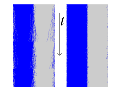
Both the hopping and resetting dynamics conserve the total number of particles, so that the half-filling condition is respected at all times, and the global particle density remains fixed at $1/2.$ Between two resetting events the time evolution of the system is governed by the hopping dynamics only. The time-scale associated with the resetting mechanism is given by $r^{-1},$ which also gives a measure of the typical duration between two consecutive resetting events. Figure 1 shows typical examples of the time evolution for two different values of the resetting rate $r.$

In the absence of resetting, the master equation governing the time-evolution of the probability ${\mathcal{P}}_{0}({\mathcal{C}},t)$ for the system to be in the configuration ${\mathcal{C}}$ at time $t$ is given by

$$\frac{\textrm{d}}{\textrm{d}t}{\mathcal{P}}_{0}({\mathcal{C}},t)={\mathcal{L}}_{0}{\mathcal{P}}_{0}({\mathcal{C}},t).$$ (2)

Here ${\mathcal{L}}_{0}$ is the Markov matrix in absence of the resetting, i.e., ${\mathcal{L}}_{0}{\mathcal{P}}_{0}({\mathcal{C}},t)=\sum_{\mathcal{C}^{\prime}}[W_{\mathcal{C^{\prime}\to C}}{\mathcal{P}}_{0}({\mathcal{C}^{\prime},t})-W_{\mathcal{C\to C^{\prime}}}{\mathcal{P}}_{0}({\mathcal{C}},t)]$ where $W_{\mathcal{C^{\prime}\to C}}$ denotes the rate for the jump $\mathcal{C\to C^{\prime}}$ due to hopping dynamics only. Note that, $W_{\mathcal{C^{\prime}\to C}}=1$ only if the two configurations $\mathcal{C}$ and $\mathcal{C^{\prime}}$ are connected by a single hop of a particle to a neighbouring site.

Let ${\mathcal{P}}({\mathcal{C}},t)$ denote the probability of finding the system in the configuration ${\mathcal{C}}$ at time $t$ in presence of resetting. In this case, the master equation reads,

$$\frac{\textrm{d}}{\textrm{d}t}{\mathcal{P}}({\mathcal{C}},t) = {\mathcal{L}}_{0}{\mathcal{P}}({\mathcal{C}},t)$$ (4)

$$+r\sum_{\mathcal{C^{\prime}\neq C}_{0}}{\mathcal{P}}({\mathcal{C}^{\prime}},t)\delta_{\mathcal{C,C}_{0}}-r{\mathcal{P}}({\mathcal{C}},t)(1-\delta_{\mathcal{C,C}_{0}})$$

$$= ({\mathcal{L}}_{0}-r){\mathcal{P}}({\mathcal{C}},t)+r\delta_{C,C_{0}},$$ (5)

where $\delta_{\mathcal{C,C}_{0}}$ is the Kronecker delta symbol, which takes the value unity when $\mathcal{C}$ is same as $\mathcal{C}_{0},$ and is zero otherwise. It is straightforward to write a formal solution of Eq. (5),

$${\mathcal{P}}({\mathcal{C}},t) = e^{(\mathcal{L}_{0}-r)t}{\mathcal{P}}(\mathcal{C},0)+r\int_{0}^{t}\textrm{d}s~{}e^{(\mathcal{L}_{0}-r)s}\delta_{C,C_{0}}$$ (6)

$$= e^{-rt}{\mathcal{P}}_{0}(\mathcal{C},t)+r\int_{0}^{t}\textrm{d}s~{}e^{-rs}{\mathcal{P}}_{0}(\mathcal{C},s).$$ (7)

Here ${\mathcal{P}}_{0}(\mathcal{C},t)=e^{\mathcal{L}_{0}t}{\mathcal{P}}(\mathcal{C},0)$ is the probability of finding the system in configuration $\mathcal{C}$ at time $t$ in the absence of resetting given that the system was initially at $\mathcal{C}_{0},$ i.e., $\mathcal{P}(\mathcal{C},0)={\mathcal{P}}_{0}(\mathcal{C},0)=\delta_{\mathcal{C},\mathcal{C}_{0}}$. Equation (7) is nothing but the renewal equation for the configuration probability, which has been obtained earlier and used to study resetting phenomena in various other contexts Brownian ; kpz-reset . Note that Eq. (7) holds true irrespective of the specific choice of $\mathcal{C}_{0}$ given in Eq. (1).

In the absence of resetting the ordinary SEP on a ring relaxes to an equilibrium state with flat density profile and zero current. The approach to the equilibrium state, starting from the step-like initial configuration ${\mathcal{C}}_{0},$ is characterized by a diffusive current flowing through the system. It has been shown that, for an infinitely large system, the time-integrated current measuring the net particle flux through the central bond up to time $t,$ grows as $\sqrt{t}$ for large $t$ Derrida1 ; Derrida2 . Presence of resetting is expected to affect these characteristics of SEP which we investigate in detail in this paper. A brief summary of our results is presented below.

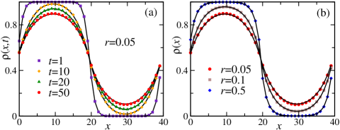
• First, we compute an exact expression for the evolution of the average density profile $\rho(x,t)=\langle s_{x}(t)\rangle$ for any arbitrary value of the resetting rate $r,$ which is given in Eq. (15). We observe that the evolution is non-trivially modified due to the presence of resetting which leads to an inhomogeneous stationary density profile [see Fig. 2(b)] in contrast to the flat one for $r=0$.

• This inhomogeneous density profile provides some characterization of the non-equilibrium state of the system. It is, however, also important to look at how the particle currents in the system are affected by the introduction of resetting. In addition to the usual diffusive current $J_{\textrm{d}}(t)$ created due to the local hopping of the particles, there is also a contribution $J_{\text{reset}}(t)$ to the total current due to the global movements of the particles during the resetting events.

  We show that the behaviour of the diffusive current changes drastically in presence of resetting. In particular, we compute the average diffusive current $\langle J_{\text{d}}(t)\rangle$ exactly, which, in the long time limit, shows a linear growth with time $t,$

  $$\langle J_{\text{d}}(t)\rangle\simeq t\sqrt{\frac{r}{r+4}}.$$

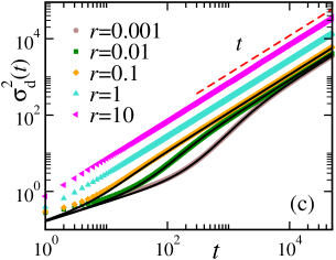
  This behaviour is in stark contrast to the $\sqrt{t}$ growth which is seen in absence of resetting Derrida1 . Similar change in the dynamical behaviour is also observed for the variance of the diffusive current, which also grows as $\sim t$ in presence of resetting, as opposed to $\sqrt{t}.$ We explore the behaviour of the resetting current $J_{\text{reset}}$ too and show that, its average and variance also grow linearly with time. We also investigate the probability distribution of $J_{\text{d}}(t)$ and demonstrate that, in the long-time regime, the typical fluctuations of $J_{\text{d}}(t)$ around its mean is characterized by a Gaussian distribution. Similar Gaussian fluctuations are also expected for the resetting current $J_{\text{reset}}.$

• Finally, we study the behaviour of the total current $J_{r}=J_{\text{d}}+J_{\text{reset}}$ and calculate the average $\langle J_{r}(t)\rangle$ and the second moment $\langle J_{r}^{2}(t)\rangle$ as functions of time $t.$ In the long-time limit the moments reach stationary values. In particular, we show that the average stationary current is given by

  $$\langle J_{r}\rangle=\frac{1}{\sqrt{r(r+4)}}.$$ (8)

  We also compute the stationary probability distribution of the total current $P_{r}^{\text{st}}(J_{r}),$ for small values of $r,$ using a renewal approach. Interestingly, it turns out that, this distribution is non-Gaussian, and has very asymmetric behaviour at the two tails.

III Density profile

Presence of repeated resetting to the inhomogeneous configuration $\mathcal{C}_{0}$ destroys the translational invariance in the system and a non-trivial density profile can be expected, even in the stationary state. The average density $\rho(x,t)=\langle s_{x}(t)\rangle$ is given by the probability that the site $x$ is occupied any time $t.$ The time-evolution equation for the density profile can be derived by multiplying Eq. (5) by $s_{x}$ and summing over all configurations $\mathcal{C},$

$$\frac{\textrm{d}}{\textrm{d}t}\rho(x,t) = \rho(x+1,t)+\rho(x-1,t)-2\rho(x,t)$$ (10)

$$-r\rho(x,t)+r\phi(x)$$

Here $\phi(x)$ is the density profile corresponding to the resetting configuration ${\mathcal{C}}_{0}$ which, as mentioned before, is also taken as the initial profile. The exact time-dependent density profile $\rho(x,t)$ can be obtained by solving Eq. (10). To this end we introduce the discrete Fourier transform

$$\tilde{\rho}(n,t)=\sum_{x=0}^{L-1}e^{i\frac{2\pi nx}{L}}\rho(x,t),\;\text{with}~{}n=0,1,2\dots L-1.~{}~{}$$ (11)

Substituting Eq. (11) in Eq. (10), we get,

$$\frac{\textrm{d}}{\textrm{d}t}\tilde{\rho}(n,t)=-(\lambda_{n}+r)\tilde{\rho}(n,t)+r\tilde{\phi}(n)$$ (12)

with $\lambda_{n}=2\left(1-\cos\frac{2\pi n}{L}\right)$ and $\tilde{\phi}(n)$ is the Fourier transform of the resetting (and initial) profile $\phi(x).$ Equation (12) can immediately be solved,

$$\tilde{\rho}(n,t)=\frac{r\tilde{\phi}(n)}{r+\lambda_{n}}+\frac{\lambda_{n}\tilde{\phi}(n)}{r+\lambda_{n}}e^{-(r+\lambda_{n})t}$$ (13)

The density profile is then obtained by inverting the Fourier transform,

$$\rho(x,t) = \frac{r}{L}\sum_{n=0}^{L-1}\frac{\tilde{\phi}(n)}{r+\lambda_{n}}e^{-i\frac{2\pi nx}{L}}$$ (15)

$$+\frac{1}{L}\sum_{n=0}^{L-1}\frac{\lambda_{n}\tilde{\phi}(n)}{r+\lambda_{n}}e^{-(r+\lambda_{n})t}e^{-i\frac{2\pi nx}{L}}$$

Figure 2: Density profile: (a) Time evolution of the density profile $\rho(x,t),$ starting from a step-like initial condition, for resetting rate $r=0.05,$ and for different values of time $t.$ The symbols correspond to the data obtained from numerical simulations and the solid lines correspond to the analytical result [see Eq. (LABEL:eq:rhor_t_C0)]. (b) The stationary density profile $\rho(x)$ for different reset rates $r.$ The symbols correspond to the data obtained from numerical simulations and the solid lines correspond to the analytical result [see Eq. (22)]. The lattice size $L=40$ for both (a) and (b).

In the stationary state, the second term decays exponentially and the stationary density profile is given by,

$$\rho(x) = \frac{r}{L}\sum_{n=0}^{L-1}\frac{\tilde{\phi}(n)}{r+\lambda_{n}}e^{-i\frac{2\pi nx}{L}}$$ (16)

$$= \frac{1}{2}+\frac{r}{L}\sum_{n=1}^{L-1}\frac{\tilde{\phi}(n)}{r+\lambda_{n}}e^{-i\frac{2\pi nx}{L}}$$ (17)

where we have used the fact that $\tilde{\phi}(0)=\sum_{x}\phi(x)=L/2.$ Clearly, in absence of resetting, i.e.for $r=0,$ we get the flat profile which corresponds to the equilibrium scenario. For non-zero $r,$ however, the stationary profile is non-trivial and corresponds to a non-equilibrium stationary state, carrying non-zero current. We will explore that in the next section.

It is worth mentioning that $\rho(x,t)$ also satisfies a renewal equation (following directly from Eq. (7)) in terms of the density profile $\rho_{0}(x,t)$ in absence of resetting,

$$\rho(x,t)=e^{-rt}\rho_{0}(x,t)+r\int_{0}^{t}\textrm{d}\tau~{}e^{-r\tau}\rho_{0}(x,\tau).$$ (18)

For the sake of completeness we have added a brief review of the density profile and its evolution for ordinary SEP in the Appendix A. Using the explicit form of $\rho_{0}(x,t)$ given in Eq. (111) it is straightforward to check that Eq. (18) leads to Eq. (15).

We have not used any specific form of $\phi(x)$ so far; in fact, the results above are valid for resetting to any generic profile. For the specific choice of the step-like configuration given in Eq. (1) we have $\phi(x)=1-\Theta(x+1-\frac{L}{2})$ and

$$\tilde{\phi}(n)=\frac{1-(-1)^{n}}{1-e^{i\frac{2\pi n}{L}}}=\left\{\begin{split}1+i~{}\cot\frac{\pi n}{L}&\qquad\text{for odd}~{}~{}~{}n\cr 0~{}~{}~{}~{}~{}&\qquad\text{for even}~{}~{}~{}n\end{split}\right.$$ (19)

In that case, the density profile takes the form,

$$\rho(x,t) = \rho(x)+\frac{1}{L}\sum_{n=1,3}^{L-1}e^{-i\frac{2\pi nx}{L}}\frac{\lambda_{n}(1+i~{}\cot\frac{\pi n}{L})}{r+\lambda_{n}}e^{-(r+\lambda_{n})t}$$ (20)

where

$$\rho(x)=\frac{1}{2}+\frac{r}{L}\sum_{n=1,3}^{L-1}e^{-i\frac{2\pi nx}{L}}\frac{(1+i~{}\text{cot}\frac{\pi n}{L})}{r+\lambda_{n}}$$ (22)

is the stationary profile.

Figure 2(a) shows the time-evolution of the density profile $\rho(x,t)$ for a specific resetting rate $r$ and Fig. 2(b) shows stationary profiles $\rho(x)$ for different values of $r.$ In both cases, the analytical results (solid lines) are compared with the data obtained from numerical simulations (symbols). An excellent match confirms our analytical prediction.

IV Particle current

The behaviour of current plays an important role in characterizing the interacting particle systems like exclusion processes. For ordinary SEP, there is no particle current flowing through the system in the stationary (equilibrium) state. However, starting from a step-like initial configuration, the relaxation to equilibrium is characterized by the presence of a non-vanishing particle current. In particular, the behaviour of the time-integrated current, i.e., the net particle flux through the central bond up to time $t,$ has been studied extensively in the past and it was shown that at long time limit, the average flux grows $\sim\sqrt{t}$ Derrida1 ; Derrida2 .

In presence of resetting, there are two different kinds of particle motions, consequently the total current can be expressed as,

$$J_{r}(t)=J_{\text{d}}(t)+J_{\text{reset}}(t)$$ (23)

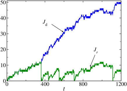
Here $J_{\text{d}}$ is net diffusive flux, i.e., the net number of particles which crossed the central bond due to the nearest neighbour hopping. $J_{\text{reset}}$ denotes the contribution due to the sudden reset to the step-like configuration $\mathcal{C}_{0}$. Note that, after a resetting, the system is brought back to $\mathcal{C}_{0}$, i.e., there are no particles to the right of the central bond, implying that the total current $J_{r}$ is also reset to zero after each resetting event. Figure 3 shows the time evolution of $J_{\text{d}}$ and $J_{r}$ for a typical trajectory of the system. The sudden jumps in $J_{r}$ indicate the resetting events.

Figure 3: Time evolution of the diffusive current $J_{\text{d}}(t)$ and the total current $J_{r}(t)$ along a typical trajectory of the system. On an average, the diffusive current increases with time $t.$ The total current vanishes after each resetting event –indicated by the vertical lines on the light green curve – and reaches a stationary state in the long time limit.

In the absence of resetting, the only source of current is the diffusive hopping motion. In the following we explore the behaviours of all these three different currents, in presence of resetting.

Figure 4: Behaviour of the diffusive current $J_{\text{d}}.$ (a) Plot of $\langle J_{\text{d}}(t)\rangle$ as a function of time $t$ for different values of $r.$ The symbols correspond to the data obtained from numerical simulations whereas the solid lines correspond to the analytical prediction [see Eq. (34)]. The lowermost curve corresponds to the smallest value of $r.$ (b) Scaling collapse of $\sqrt{r}\langle J_{\text{d}}(t)\rangle$ for small $r$ according to Eq.  (37); the solid line corresponds to the predicted scaling function. (c) Plot of the variance $\sigma_{\textrm{d}}^{2}(t)$ vs $t$ for different values of $r.$ The curves corresponding to small values of $r$ (three lower curves) are compared with the analytical predictions (solid lines). A lattice of size $L=1000$ is used here for the numerical simulations.

IV.1 Diffusive current

The diffusive current $J_{\text{d}}(t)$ measures the total number of particles which crossed the central bond $(\frac{L}{2}-1,\frac{L}{2})$ during the time interval $[0,t],$ and can be expressed as a time integral,

$$J_{\text{d}}(t) = \int_{0}^{t}\textrm{d}s~{}j(s)$$ (24)

Here, $j(t)$ denotes the instantaneous diffusive current, i.e., the number of particles crossing the central bond during the time-interval $t$ and $t+\textrm{d}t.$ The average instantaneous current is given by,

$$\langle j(t)\rangle = \left\langle s_{\frac{L}{2}-1}(1-s_{\frac{L}{2}})\right\rangle-\left\langle(1-s_{\frac{L}{2}-1})s_{\frac{L}{2}}\right\rangle$$ (25)

$$= \rho\left(\frac{L}{2}-1,t\right)-\rho\left(\frac{L}{2},t\right)$$ (26)

Using the explicit expression for the density from eq. (LABEL:eq:rhor_t_C0) one gets,

$$\langle j(t)\rangle=\frac{2}{L}\sum_{n=1,3}^{L-1}\bigg{[}\frac{r}{r+\lambda_{n}}+\frac{\lambda_{n}}{r+\lambda_{n}}e^{-(r+\lambda_{n})t}\bigg{]}.$$ (27)

In the limit of thermodynamically large system size, i.e.$L\to\infty$, the sum in the above expression can be converted to an integral over continuous variable $q=2\pi n/L$ and we get,

$$\langle j(t)\rangle=\int_{0}^{2\pi}\frac{\textrm{d}q}{2\pi}\bigg{[}\frac{r}{r+\lambda_{q}}+\frac{\lambda_{q}}{r+\lambda_{q}}e^{-(r+\lambda_{q})t}\bigg{]}$$ (28)

where $\lambda_{q}=2(1-\cos q).$ In the long-time regime, the second term decays exponentially and $\langle j(t)\rangle$ reaches a stationary value,

$$\lim_{t\to\infty}\langle j(t)\rangle=\int_{0}^{2\pi}\frac{\textrm{d}q}{2\pi}\frac{r}{r+2(1-\cos q)}=\sqrt{\frac{r}{r+4}}.$$ (29)

The average net flux $\langle J_{\text{d}}(t)\rangle$ up to time $t$ can be found by integrating the instantaneous current,

$$\langle J_{\text{d}}(t)\rangle = \sqrt{\frac{r}{r+4}}t$$ (30)

$$+ \int_{0}^{2\pi}\frac{\textrm{d}q}{2\pi}\frac{\lambda_{q}}{(r+\lambda_{q})^{2}}(1-e^{-(r+\lambda_{q})t}).$$ (31)

Clearly, in the long-time regime, the second term goes to a constant and the first term dominates the behaviour of the average current which grows linearly with time,

$$\langle J_{\text{d}}(t)\rangle\simeq\sqrt{\frac{r}{r+4}}t.$$ (32)

This equation is one of our main results, which shows that the behaviour of the diffusive current changes drastically by the presence of resetting; instead of the standard $\sqrt{t}$ growth in a diffusive system, resetting yields a much faster, linear, temporal growth of the diffusive current. The average current $\langle J_{\text{d}}(t)\rangle$ at any time $t,$ i.e., before reaching the $\sim t$ behaviour, can be obtained from Eq. (31) by evaluating the $q$-integral numerically. In fact, one can also derive an alternative expression which lends itself more easily to numerical evaluation. Let us recall that the density profile $\rho(x,t)$ satisfies a renewal equation (18) for any $x$. Then, clearly, $\langle j(t)\rangle$ must also satisfy the same renewal equation,

$$\langle j(t)\rangle = e^{-rt}\langle j_{0}(t)\rangle+r\int_{0}^{t}\textrm{d}\tau~{}e^{-r\tau}\langle j_{0}(\tau)\rangle$$ (33)

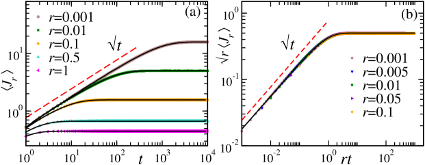
where $j_{0}(t)$ denotes instantaneous current through the central bond in the absence of resetting. The average instantaneous current is given by $\langle j_{0}(t)\rangle=e^{-2t}I_{0}(2t)$ where $I_{0}$ is the Modified Bessel function of the first kind (see Appendix B for the details). The average diffusive net current is obtained by integrating the above equation w.r.t. time [see Eq. (24)],

$$\langle J_{\text{d}}(t)\rangle = \int_{0}^{t}\textrm{d}\tau~{}e^{-r\tau}(1+rt-r\tau)\langle j_{0}(\tau)\rangle.\;\;$$ (34)

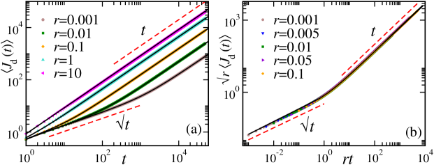
It is straightforward to show that Eq. (34) is equivalent to Eq. (31). Average current $\langle J_{\text{d}}(t)\rangle$ computed from Eq. (34), for different values of $r,$ are plotted together with the same obtained from simulation in Figure 4(a).

An explicit form for $\langle J_{\text{d}}(t)\rangle$ can be derived for small $r\ll 1.$ Using a variable transformation $w=r\tau,$ and using the exact form for $\langle j_{0}(\tau)\rangle$ we get,

$$\langle J_{\text{d}}(t)\rangle = \frac{1}{r}\int_{0}^{rt}\textrm{d}w(1+rt-w)e^{-w}e^{-\frac{2w}{r}}I_{0}\left(\frac{2w}{r}\right).\;\;\;$$ (35)

For small $r,$ the argument of $I_{0}$ is large and one can use the asymptotic form for the Modified Bessel function given in Eq.  (117),

$$\langle J_{\text{d}}(t)\rangle \simeq \frac{1}{r}\int_{0}^{rt}\textrm{d}w(1+rt-w)e^{-w}\frac{1}{2\sqrt{\pi w/r}}$$ (36)

$$= \frac{1}{2\sqrt{r}}\bigg{[}\left(rt+\frac{1}{2}\right)\text{erf}(\sqrt{rt})+\sqrt{\frac{rt}{\pi}}e^{-rt}\bigg{]}.$$ (37)

In the short time-regime this function grows as $\sqrt{t}$ which is reminiscent of the free SEP and crosses over to the linear behaviour for $t\gg r^{-1}.$ Figure 4(b) shows plot of $\sqrt{r}\langle J_{\text{d}}(t)\rangle$ as a function of $rt$ for different small values of $r$ which shows a perfect collapse and matches with the scaling function given by the above equation.

To characterize the fluctuation of the diffusive current we next calculate the second moment of $J_{\text{d}}.$ The above renewal equation method cannot be applied directly to compute higher order moments. To this end, we now adopt a different approach. Let us assume that there are $n$ resetting events during the time interval $[0,t];$ moreover, let $t_{i}$ denote the interval between $(i-1)^{th}$ and $i^{th}$ events, so that $\sum_{i=1}^{n+1}t_{i}=t.$ Note that, $t_{n+1}$ denotes the time-interval between the last reset and the final time $t.$ Let us also recall that between two consecutive resetting events the system evolves following ordinary SEP dynamics. The diffusive current during the interval $[0,t]$ can, then, be expressed as,

$$J_{\text{d}}=\sum_{i=1}^{n+1}J_{0}(t_{i}),$$ (38)

where, $J_{0}(t_{i})$ are independent of each other. For notational convenience, we denote $J_{i}\equiv J_{0}(t_{i}).$ The probability density that the diffusive current will have a value $J_{\text{d}}$ in time $t$ is then given by

$$P(J_{\text{d}},t) = \sum_{n=0}^{\infty}\int_{0}^{t}\prod_{i=1}^{n+1}\textrm{d}t_{i}~{}{\mathcal{P}}_{n}(\{t_{i}\};t)$$ (40)

$$\times\int\prod_{i=1}^{n+1}\textrm{d}J_{i}P_{0}(J_{i},t_{i})~{}\delta(J_{\text{d}}-\sum_{i}J_{i}),\quad\text{where,}$$

$${\mathcal{P}}_{n}(\{t_{i}\};t) = r^{n}e^{-r\sum_{i=1}^{n+1}t_{i}}\delta(t-\sum_{i}t_{i})$$ (41)

denotes the probability of having $n$ resetting events with duration $t_{i}$ within the interval $[0,t].$ The distribution of the individual $J_{i}$-s are denoted by $P_{0}(J_{i},t_{i})$ which is exactly the distribution of the diffusive current in SEP, in the absence of resetting.

To handle the constraints presented by the $\delta$-functions, it is convenient to calculate the Laplace transform w.r.t. time $t$ of the moment generating function $\langle e^{\lambda J_{\text{d}}}\rangle,$

$$Q(s,\lambda) = {\mathcal{L}}_{t\to s}[\langle e^{\lambda J_{\text{d}}}\rangle]=\int_{0}^{\infty}\textrm{d}t~{}e^{-st}\langle e^{\lambda J_{\text{d}}}\rangle$$ (42)

$$= \int_{0}^{\infty}\textrm{d}t~{}e^{-st}\int\textrm{d}J_{\text{d}}~{}e^{\lambda J_{\text{d}}}P(J_{\text{d}},t).$$ (43)

Using Eq. (41), and performing the integrals over $J_{\text{d}}$ and $t,$ we get,

$$Q(s,\lambda) = \sum_{n=0}^{\infty}r^{n}\int_{0}^{\infty}\prod_{i}^{n+1}\textrm{d}t_{i}\exp{\bigg{[}-(r+s)\sum_{i=1}^{n+1}t_{i}\bigg{]}}$$ (44)

$$\times\int\prod_{i}^{n+1}\textrm{d}J_{i}\exp{\bigg{[}\lambda\sum_{i=1}^{n+1}J_{i}\bigg{]}}P_{0}(J_{i},t_{i})$$

$$= \sum_{n=0}^{\infty}r^{n}h(s,\lambda)^{n+1}$$ (45)

where, we have denoted,

$$h(s,\lambda)=\int_{0}^{\infty}\textrm{d}\tau~{}e^{-(r+s)\tau}\int\textrm{d}J_{0}~{}e^{\lambda J_{0}}P_{0}(J_{0},\tau)$$ (46)

Performing the sum in Eq. (45), we get,

$$Q(s,\lambda)=\frac{h(s,\lambda)}{1-rh(s,\lambda)}$$ (47)

which gives a simple relation between the moment generating functions of the current in the presence and absence of resetting. To calculate $h(s,\lambda)$ we need the current distribution $P_{0}(J_{0},\tau)$ for the ordinary SEP, which is not known in general for arbitrary values of $\tau$. However, for small values of $r$ and $s,$ the $\tau$-integral in Eq. (46) is dominated by large values of $\tau,$ and in that case one can use the result of Ref. Derrida1 where the authors have derived an expression for the moment generating function of $J_{0}(\tau)$ in the large time limit. Adapting their result to our specific case (see Appendix B.1 for the details), we have,

$$\int\textrm{d}J_{0}~{}e^{\lambda J_{0}}P_{0}(J_{0},\tau)=\langle e^{\lambda J_{0}}\rangle\simeq e^{\sqrt{\tau}F(\lambda)},$$ (48)

with,

$$F(\lambda)=-\frac{1}{\sqrt{\pi}}\text{Li}_{3/2}(1-e^{\lambda}).$$ (49)

Here $\text{Li}_{\alpha}(z)$ denotes the Poly-Logarithm function (see Ref. polylog , Eq. 25.12.10). Substituting Eq. (48) in Eq. (46) and performing the integral over $\tau,$ we get, for small $r$ and $s,$

$$h(s,\lambda) = \frac{1}{r+s}\bigg{[}1+\frac{\sqrt{\pi}F(\lambda)}{2\sqrt{r+s}}e^{\frac{F(\lambda)^{2}}{4(r+s)}}\bigg{(}1+\text{erf}\bigg{[}\frac{F(\lambda)}{2\sqrt{r+s}}\bigg{]}\bigg{)}\bigg{]}$$ (50)

One can easily extract the Laplace transforms of the moments using Eq. (LABEL:eq:hsl_F) along with (47). First, we have,

$${\mathcal{L}}_{t\to s}\left[\langle J_{\text{d}}(t)\rangle\right] = \frac{\textrm{d}}{\textrm{d}\lambda}Q(s,\lambda)\bigg{|}_{\lambda=0}$$ (52)

$$= \frac{\sqrt{r+s}}{2s^{2}}$$ (53)

The average current can be obtained by inverting the Laplace transform,

$$\mu_{\textrm{d}}(t)\equiv\langle J_{\text{d}}(t)\rangle = {\mathcal{L}}^{-1}_{s\to t}\left[\frac{\sqrt{r+s}}{2s^{2}}\right]$$ (54)

The inversion can be performed exactly using Mathematica, and yields,

$$\mu_{\textrm{d}}(t) = \frac{1}{2\sqrt{r}}\bigg{[}\left(rt+\frac{1}{2}\right)\text{erf}(\sqrt{rt})+\sqrt{\frac{rt}{\pi}}e^{-rt}\bigg{]}$$ (55)

Note that the above equation is the same as Eq. (37), which was obtained using a different method.

Figure 5: Distribution of the diffusive current $P(J_{\textrm{d}},t)$ for $r=0.01$: (a) Plot of $P(J_{\textrm{d}},t)$ vs $J_{\text{d}}$ for different values of $t,$ the left most curve corresponding to the smallest value of $t.$ The solid lines correspond to the predicted Gaussian form (61). (b) The same data are plotted as a function of $(J_{\textrm{d}}-\mu_{\textrm{d}})/\sigma_{d}.$ The solid black line corresponds to a standard normal distribution ${\mathcal{N}}(0,1).$

The Laplace transform of the second moment is obtained from the second derivative of $Q(s,\lambda),$

$${\mathcal{L}}_{t\to s}\langle J_{\text{d}}^{2}(t)\rangle = \frac{\textrm{d}^{2}}{\textrm{d}\lambda^{2}}Q(s,\lambda)\bigg{|}_{\lambda=0}$$ (56)

$$= \frac{1}{\pi s^{2}}+\frac{b\sqrt{r+s}}{2s^{2}}+\frac{r}{2s^{3}}$$ (57)

where $b=(1-1/\sqrt{2}).$ Fortunately, the inverse Laplace transform can be performed exactly in this case also, and it yields, for small $r,$

$$\langle J_{\text{d}}^{2}(t)\rangle = \frac{1}{4\pi}\bigg{[}t(\pi rt+4)+2b\sqrt{\pi t}e^{-rt}$$ (59)

$$\quad+\frac{b\pi}{\sqrt{r}}(1+2rt)\text{erf}(\sqrt{rt})\bigg{]}$$

Note that, the above expression is expected to be valid for large $t,$ as we have assumed $s$ to be small. The variance of the diffusive current $\sigma^{2}_{\text{d}}(t)=\langle J_{\text{d}}^{2}(t)\rangle-\langle J_{\text{d}}(t)\rangle^{2}$ can be obtained using Eqs. (55) and (59). In particular, in the long time limit, the variance increases linearly with time $t$, and is given by,

$$\sigma_{\text{d}}^{2}(t)\simeq t\bigg{[}\frac{4-\pi}{4\pi}+\frac{\sqrt{r}}{2}\bigg{(}1-\frac{1}{\sqrt{2}}\bigg{)}\bigg{]}$$ (60)

Figure 4(c) shows a plot of $\sigma^{2}_{\text{d}}(t)$ vs $t$ for different values of $r,$ obtained from numerical simulations; all the curves show linear growth in the long time regime. The curves corresponding to small values of $r\ll 1$ are compared with the analytical result (solid lines) which shows a perfect match for $t>10.$

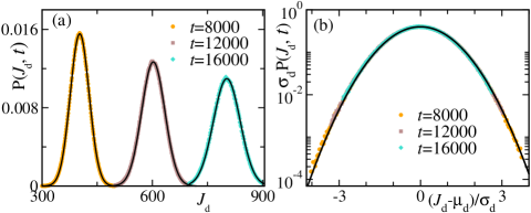
Distribution of $J_{\text{d}}$: It is interesting to investigate the probability distribution of the diffusive current $J_{d}(t)$. From Eq. (38) we observe that $J_{d}(t)$ is the sum of the hopping currents $J_{0}(t_{i})$ between successive resetting events. Since the time-evolution of the system is Markovian and after each resetting event the system is brought back to the initial configuration, the variables $J_{0}(t_{i})$ are independent and distributed identically . As mentioned earlier, the distribution of $J_{0}(t_{i})$ is known Derrida1 and has finite moments. Over a large time interval $t$, the number $n$ of resetting events, which is also a random quantity, is typically large and on an average grows linearly with time $t;$ in fact, $\langle n\rangle=rt.$ For $t\gg r^{-1},$ $J_{\text{d}}(t)$ is a sum of large number of independent random variables. Hence, by central limit theorem, one can expect that for large $t$, the typical distribution of $J_{d}$ would be a Gaussian:

$$P(J_{\text{d}},t)\simeq\frac{1}{\sqrt{2\pi\sigma_{d}^{2}(t)}}\exp\left(-\frac{[J_{d}-\mu_{\textrm{d}}(t)]^{2}}{2\sigma_{d}^{2}(t)}\right)$$ (61)

where the mean $\mu_{\textrm{d}}(t)$ and the variance $\sigma_{d}^{2}(t)$ are given in Eqs. (55) and (60) respectively. This prediction is verified in Fig. 5(a) where the Gaussian form of $P(J_{\text{d}},t)$ is compared to the data obtained from numerical simulations for a set of (large) values of $t$ and fixed $r.$ Clearly, the analytical curves are indistinguishable from the simulation data, which confirms our prediction. Fig. 5(b) shows the same data plotted against the scaled variable $(J_{\text{d}}-\mu_{d}(t))/\sigma_{d}(t)$ and compared with the standard normal distribution (solid black line).

IV.2 Resetting current

Presence of the resetting dynamics gives rise to a resetting current $J_{\text{reset}}$ [see Eq. (23)] which measures the flow of particles due to the sudden change in the configuration of the system. In this Section we investigate the properties of this resetting current. Let us remember that the number of particles crossing the central bond (from right to left) at the resetting event is exactly same as the hopping current (from left to right) during the period after the previous resetting event. Net resetting current during a time interval $[0,t],$ then, can be expressed as,

$$J_{\text{reset}}=-\sum_{i=1}^{n}{J_{0}(t_{i})}$$ (62)

where, as before, $n$ denotes the number of resetting events in time $t$ and $t_{i}$ denotes the interval between $(i-1)^{th}$ and $i^{th}$ resetting events. Note that, the upper limit of the sum is $n$ in the above Eq. (62) as there is no contribution to the resetting current after the last resetting event.

Figure 6: Behaviour of the resetting current $J_{\text{reset}}:$ (a) Plot of $-\langle J_{\text{reset}}(t)\rangle$ as a function of time for different values of $r$ obtained from numerical simulations. The lowermost curve corresponds to the smallest value of $r.$ The black solid lines correspond to the analytical prediction Eq. (70) for small values of $r.$ (b) Variance of the resetting current $\langle\sigma^{2}_{\text{reset}}(t)\rangle$ as a function of time $t$ for different values of $r.$ The curves corresponding to small values of $r$ (three lower curves) are compared with the analytical result (black solid lines). A lattice of size $L=1000$ is used for all the numerical simulations.

To calculate the moments of $J_{\text{reset}}$ we follow the same method as in Sec. IV.1 and calculate the Laplace transform of the moment generating function of $J_{\text{reset}},$

$$K(s,\lambda)=\int_{0}^{\infty}\textrm{d}t~{}e^{-st}\int\textrm{d}J_{\text{reset}}e^{\lambda J_{\text{reset}}}\mathscr{P}(J_{\text{reset}},t).~{}~{}$$ (63)

Here $\mathscr{P}(J_{\text{reset}},t)$ denotes the probability that the resetting current has a value $J_{\text{reset}}$ at time $t,$ and is given by,

$$\mathscr{P}(J_{\text{reset}},t) = \sum_{n=0}^{\infty}\int_{0}^{t}\prod_{i=1}^{n+1}\textrm{d}t_{i}~{}{\mathcal{P}}_{n}(\{t_{i}\};t)$$ (64)

$$\times \int\prod_{i=1}^{n}\textrm{d}J_{i}P_{0}(J_{i},t_{i})~{}\delta(J_{\text{reset}}+\sum_{i=1}^{n}J_{i}).~{}~{}$$ (65)

with ${\mathcal{P}}_{n}(\{t_{i}\};t)$ given in Eq. (41). As before, we have used $J_{i}\equiv J_{0}(t_{i}).$ Using Eq. (65) in Eq. (63) and performing the integrals over $t$ and $J_{\text{reset}},$ we get,

$$K(s,\lambda) = \frac{1}{(r+s)}\sum_{n=0}^{\infty}r^{n}h(s,-\lambda)^{n}$$ (66)

$$= \frac{1}{(r+s)[1-rh(s,-\lambda)]}$$ (67)

where $h(s,\lambda)$ is given by Eq. (46). As mentioned already, it can computed exactly for small values of $r,s$ and is given by Eq. (LABEL:eq:hsl_F).

Next we calculate the moments of the resetting current using Eqs. (67) along with Eq. (LABEL:eq:hsl_F). First, we have the Laplace transform of the average resetting current,

$$\mathcal{L}_{t\to s}[\langle J_{\text{reset}}(t)\rangle] = \frac{\textrm{d}}{\textrm{d}\lambda}K(s,\lambda)\bigg{|}_{\lambda=0}$$ (68)

$$= -\frac{r}{2s^{2}\sqrt{r+s}}.$$ (69)

The inverse transform can be performed exactly to obtain,

$$\langle J_{\text{reset}}(t)\rangle=-\frac{1}{2\sqrt{r}}\bigg{[}(rt-\frac{1}{2})\text{erf}(\sqrt{rt})+\sqrt{\frac{rt}{\pi}}e^{-rt}\bigg{]}.~{}~{}$$ (70)

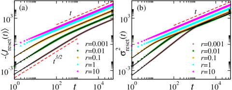
Note that the above expression is expected to be valid for small values of $r\ll 1$ and large $t\gg 1.$ Equation (70) is very similar to Eq. (55), which gives the average diffusive current $\langle J_{\text{d}}(t)\rangle$, except, of course, the fact that the average reseting current is negative. In fact, at very long-times $t\gg r^{-1},$ we see a linear growth in magnitude,

$$\langle J_{\text{reset}}(t)\rangle=-\langle J_{\text{d}}(t)\rangle\simeq-\frac{\sqrt{r}t}{2},$$ (71)

At short-times, however, a different behaviour is seen. From Eq. (70), for $t\ll r^{-1},$ we have,

$$\langle J_{\text{reset}}(t)\rangle=-\frac{2rt^{3/2}}{3\sqrt{\pi}}+\mathcal{O}(t^{5/2}).$$ (72)

Clearly, at short-times, the resetting current grows much faster than the diffusive current. Figure 6(a) shows a plot of $\langle J_{\text{reset}}(t)\rangle$ as a function of $t$ for different values of $r$ which illustrates these features.

It is also interesting to look at the fluctuations of $J_{\text{reset}}.$ From Eq. (67) we can find the Laplace transform of the second moment,

$$\mathcal{L}_{t\to s}[\langle J_{\text{reset}}^{2}(t)\rangle] = \frac{\textrm{d}^{2}}{\textrm{d}\lambda^{2}}K(s,\lambda)\bigg{|}_{\lambda=0}$$ (73)

$$= \frac{br}{2s^{2}\sqrt{r+s}}+\frac{r(\pi r+2s)}{2\pi s^{3}(r+s)}$$ (74)

where, as before, we have used $b=1-\frac{1}{\sqrt{2}}.$ Once again, the Laplace transform can be inverted exactly and yields, for $r\ll 1$ and $t\gg 1,$

$$\langle J_{\text{reset}}^{2}(t)\rangle = \frac{1}{4\pi r}\bigg{[}2e^{-rt}(2-\pi+br\sqrt{\pi t})+\pi-r+4rt$$ (75)

$$+ \pi(rt-1)^{2}+b\pi\sqrt{r}(2rt-1)\text{erf}(\sqrt{rt})\bigg{]}.$$ (76)

The variance of the resetting current $\sigma_{\text{reset}}^{2}(t)=\langle J_{\text{reset}}^{2}(t)\rangle-\langle J_{\text{reset}}(t)\rangle^{2}$ can be computed from Eqs. (76) and (70) and it turns out that the variance also increases linearly at the long time limit $t\gg r^{-1}$. In fact, it is straightforward to show that, in this limit, $\sigma_{\text{reset}}^{2}(t)=\sigma_{\textrm{d}}^{2}(t)$ [see Eq. (60)]. Figure 6(b) shows $\sigma_{\text{reset}}^{2}(t)$ for different values of $r$ obtained from numerical simulations together with the analytical prediction for small $r.$

We conclude the discussion about the resetting current with a brief comment about the probability distribution $\mathscr{P}(J_{\text{reset}},t).$ Since $J_{\text{reset}},$ similar to $J_{\text{d}}$, is also a sum of a set of independent variables $J_{0}(t_{i})$, we can use the central limit theorem to predict the behaviour of the corresponding distribution. In fact, for $rt\gg 1,$ one can expect that $\mathscr{P}(J_{\text{reset}},t)$ is similar to $P(J_{\text{d}},t)$ and has a Gaussian behaviour around the mean value,

$$\mathscr{P}(J_{\text{reset}},t)\simeq\frac{1}{\sqrt{2\pi\sigma^{2}_{\text{reset}}(t)}}\exp\bigg{[}-\frac{(J_{\text{reset}}-\langle J_{\text{reset}}(t)\rangle)^{2}}{2\sigma_{\text{reset}}^{2}(t)}\bigg{]}.$$

IV.3 Total current

In this section we investigate the behaviour of the total current $J_{r},$ as defined in Eq. (23). $J_{r}(t)$ measures the net number of particles which have crossed the central bond towards right (by hopping, or due to resetting) up to time $t.$ As already mentioned, $J_{r}$ is set to zero after every resetting event; the contribution to the total current comes only from the diffusion of the particles after the last resetting event. Consequently, one can write a renewal equation for $P_{r}(J_{r},t),$ the probability that, at time $t,$ the total current will have a value $J_{r},$

$$P_{r}(J_{r},t)=e^{-rt}P_{0}(J_{r},t)+r\int_{0}^{t}\textrm{d}s~{}e^{-rs}P_{0}(J_{r},s).$$ (77)

Here $P_{0}(J_{r},s)$ denotes the probability that, starting from $\mathcal{C}_{0},$ in absence of resetting, $J_{r}$ number of particles cross the central bond until time $s.$ We will use the above equation to explore $P_{r}(J_{r},t),$ but, first it is useful to investigate the mean and the variance of the total current.

It is easy to see that all moments of $J_{r}$ should also satisfy a renewal equation similar to Eq. (77). In particular, the average total current must satisfy,

$$\langle J_{r}(t)\rangle=e^{-rt}\langle J_{0}(t)\rangle+r\int_{0}^{t}\textrm{d}\tau~{}e^{-r\tau}\langle J_{0}(\tau)\rangle$$ (78)

where $\langle J_{0}(t)\rangle$ is the average current in absence of resetting, and is given by Eq. (116). Unfortunately, the above integral in Eq. (78) cannot be computed analytically. However, it is possible to numerically evaluate the integral and get $\langle J_{r}(t)\rangle$ for any time $t.$ This is shown in Fig. 7 for different values of $r$ and compared with numerical simulations (symbols) which matches perfectly at all times.

Figure 7: Behaviour of the total current $J_{r}:$ (a) Plot of average total current $\langle J_{r}(t)\rangle$ as a function of time for different values of $r,$ with the uppermost curve corresponding to the smallest value of $r.$ Solid lines and symbols correspond to the analytical result and data from numerical simulations, respectively. (b) Plot of $\sqrt{r}\langle J_{r}(t)\rangle$ as a function of the scaled variable $rt,$ for small values of $r.$ The solid line corresponding to the scaling function $\text{erf}(\sqrt{rt})/2$ [see Eq. (80)] (c) Second moment of the total current $\langle J^{2}_{r}(t)\rangle$ as a function of time $t$ for different values of $r.$ The curves corresponding to small values of $r$ (three upper curves) are compared with the analytical result Eq. (87) (solid lines). A lattice of size $L=1000$ is used for all the numerical simulations.

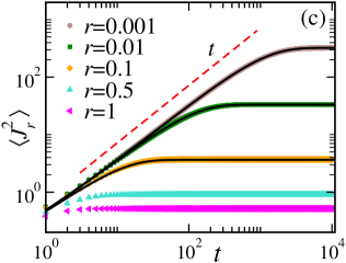
For small values of $r,$ a more explicit expression for the average total current $\langle J_{r}(t)\rangle$ can be derived. In that case, it is convenient to rewrite Eq. (78) as

$$\langle J_{r}(t)\rangle=e^{-rt}\langle J_{0}(t)\rangle+\int_{0}^{rt}\textrm{d}u~{}e^{-u}\left\langle J_{0}\left(\frac{u}{r}\right)\right\rangle$$ (79)

The integral is dominated by the contribution from small $u\sim\mathcal{O}(1);$ consequently, $u/r$ is large for small $r,$ and we can use the asymptotic expression $\langle J_{0}(u/r)\rangle\simeq\sqrt{u/r\pi}.$ Substituting that in the above equation, and performing the integral, we get, for large $t,$

$$\langle J_{r}(t)\rangle=\frac{1}{2\sqrt{r}}\text{erf}(\sqrt{rt}).$$ (80)

Equation (80) provides an explicit expression for the average total current for small $r,$ and in the large time regime. Note that, $\langle J_{r}(t)\rangle$ given by the above equation is same as $\langle J_{\text{d}}(t)\rangle+\langle J_{\text{reset}}(t)\rangle,$ as clearly seen from Eqs. (55) and (70). This is expected as the total current is a sum of the diffusive current and the resetting current [see Eq. (23)].

We have also measured the total current $J_{r}$ from numerical simulations. Figure 7(b) shows a plot of $\sqrt{r}\langle J_{r}(t)\rangle$ as a function of $rt$ for different (small) values of $r,$ as obtained from numerical simulation; the solid line corresponds to $\text{erf}(\sqrt{rt}).$ The perfect collapse of all the curves verifies our analytical prediction.

From Eq. (80) it can be seen that for $t\ll r^{-1}$ the average total current grows as $\sqrt{t},$ which is a signature of the ordinary SEP. On the other hand, in the large time limit $\langle J_{r}\rangle$ reaches a stationary value $1/2\sqrt{r}.$

In fact, the stationary value of the average total current $\langle J_{r}\rangle$ can be calculated exactly from Eq. (78) for any value of $r.$ As we have already seen, at large times $t,$ $\langle J_{0}(t)\rangle\sim\sqrt{t},$ hence, the first term in Eq. (78) decays exponentially and the large-time behaviour of the average total current is dominated by the second integral in the above equation. Recalling Eq. (116) and using the series expansion of the Modified Bessel functions $I_{0}$ and $I_{1},$ (see Ref. polylog , Eq. 10.25.2) we have,

$$\int_{0}^{t}\textrm{d}\tau~{}e^{-r\tau}\langle J_{0}(\tau)\rangle$$ (81)

$$= \sum_{m=0}^{\infty}\frac{1}{m!(m+1)!}\frac{1}{(r+2)^{2m+3}}\bigg{[}\Gamma_{2m+3}-\Gamma_{2m+3}\big{[}(r+2)t\big{]}$$ (83)

$$+~{}(r+2)(m+1)\bigg{(}\Gamma_{2m+2}-\Gamma_{2m+2}[(r+2)t]\bigg{)}\bigg{]},$$

where $\Gamma_{n}$ and $\Gamma_{n}(x)$ are the Gamma function and the incomplete Gamma function, respectively. $\Gamma_{n}(x)$ decays to zero for large $x$ for all values of $n,$ and hence, in the long time limit we have the contributions only from the $t$-independent terms,

$$\lim_{t\to\infty}\langle J_{r}\rangle \simeq r\sum_{m=0}^{\infty}\frac{(2m+1)!}{m!(m+1)!}\frac{(m+1)(r+2)+2m+2}{(r+2)^{2m+3}}$$ (84)

$$= \frac{1}{\sqrt{r(r+4)}}.$$ (85)

Clearly, in the long-time limit the average total current reaches a stationary value $\mu_{r}=1/{\sqrt{r(r+4)}}$ which decreases as the resetting rate $r$ is increased. For small $r,$ $\mu_{r}\approx\frac{1}{2\sqrt{r}}$ which is same as what we obtained by taking $t\to\infty$ limit in Eq. (80). On the other hand, for large $r\gg 1,$ $\mu_{r}$ approaches $1/r.$

Physically, the limiting behaviours of the stationary value of the average total current can be understood from the following argument. Since the value of $J_{r}$ is reset to zero after each resetting event, the final contribution to $J_{r}$ comes only from the diffusion of particles after last resetting event. Moreover, the typical duration since the last resetting event is $\tau_{r}\sim 1/r.$ For small $r,$ this typical duration is long, and the average diffusive current (without resetting) during this period is $\sim\sqrt{\tau_{r}}=1/\sqrt{r}.$ On the other hand, for large $r,$ $\tau_{r}$ is small, the diffusive current is $\sim\tau_{r}=1/r.$

Next we calculate the second moment of the total current $\langle J_{r}(t)^{2}\rangle.$ As mentioned already, the second moment also satisfies a renewal equation of the form,

$$\langle J_{r}(t)^{2}\rangle=e^{-rt}\langle J^{2}_{0}(t)\rangle+r\int_{0}^{t}\textrm{d}\tau~{}e^{-r\tau}\langle J^{2}_{0}(\tau)\rangle.$$ (86)

The above equation is valid at all times and for all values of $r.$ Unfortunately, however, the behaviour of $\langle J^{2}_{0}(\tau)\rangle$ is known only for long time $\tau$ (see Eq. (119)) so we are not able to calculate an exact analytical expression for $\langle J_{r}(t)^{2}\rangle$ for any arbitrary time $t.$ Nevertheless, one can use Eq. (86) along with Eqs. (118) and (119) to calculate $\langle J_{r}(t)^{2}\rangle$ for small values of $r,$ where the integral in Eq. (86) is dominated by the contribution from large $\tau\gg r^{-1}.$ This exercise leads to a simple analytical formula for the second moment for small $r$ (and large time $t$),

$$\langle J^{2}_{r}(t)\rangle\simeq\frac{1}{\pi r}\left(1-e^{-rt}\right)+\frac{1}{2\sqrt{r}}\left(1-\frac{1}{\sqrt{2}}\right)\text{erf}(\sqrt{rt})\qquad$$ (87)

Figure 7(c) shows the plot of $\langle J_{r}^{2}(t)\rangle$ as a function of $t$ for different values of $r.$ The curves for small $r$ are compared with the analytical result Eq. (87) which show an excellent match. Similar to the average total current, the second moment $\langle J_{r}^{2}(t)\rangle$ also eventually reaches a stationary value which, for small values of $r,$ can be obtained by taking $\lim t\to\infty$ in Eq. (87),

$$\langle J_{r}^{2}\rangle=\frac{1}{\pi r}+\frac{1}{2\sqrt{r}}\left(1-\frac{1}{\sqrt{2}}\right).$$ (88)

One can immediately calculate the stationary value of the variance $\sigma_{r}^{2}=\langle J_{r}^{2}\rangle-\langle J_{r}\rangle^{2};$ as $r\to 0,$ $\sigma_{r}^{2}\simeq(4-\pi)/4\pi r.$

On the other hand, for short time $t,$ we have,

$$\langle J_{r}^{2}(t)\rangle\simeq\frac{t}{\pi}+\sqrt{\frac{t}{\pi}}\left(1-\frac{1}{\sqrt{2}}\right)$$ (89)

At very short-times, one expects a $\sqrt{t}$ behaviour which crosses over to a linear behavior as $t$ is increased. This is also seen in Figure 7(c), where the approach to the stationary value appears predominantly linear.

Correlation between $J_{\text{d}}$ and $J_{\text{reset}}$: The computation of the second moment of the total current $J_{r}$ provides a way to estimate the correlation between the diffusive and resetting components of the current. From the definition of the total current Eq. (23), we get,

$$\langle J_{r}^{2}(t)\rangle=\langle J_{\text{d}}^{2}(t)\rangle+\langle J_{\text{reset}}^{2}(t)\rangle+2\langle J_{\text{d}}(t)J_{\text{reset}}(t)\rangle.$$ (90)

The connected correlation $C(t)=\langle J_{\text{d}}(t)J_{\text{reset}}(t)\rangle-\langle J_{\text{d}}(t)\rangle\langle J_{\text{reset}}(t)\rangle$ is then given by,

$$C(t)=\frac{1}{2}\bigg{[}\sigma_{r}^{2}(t)-\sigma_{\textrm{d}}^{2}(t)-\sigma_{\text{reset}}^{2}(t)\bigg{]}$$ (91)

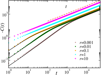
where $\sigma_{r}^{2},\sigma_{\textrm{d}}^{2}$ and $\sigma_{\text{reset}}^{2}$ are the variances of the total, diffusive and resetting currents, respectively. Using Eqs.  (87), (59), and (76) along with Eqs. (80), (55) and (70), we get, for small values of $r,$

$$C(t) = \frac{1}{4\pi r}\Bigg{[}4-\pi+rte^{-2rt}$$ (92)

$$+ e^{-rt}\left(\pi-4-2r\sqrt{\pi t}[b-\sqrt{r}t~{}\text{erf}(\sqrt{rt})]\right)$$ (93)

$$- rt(4-\pi+\pi rt)-b\pi\sqrt{r}(2rt-1)\text{erf}(\sqrt{rt})$$ (94)

$$+ \pi\left(r^{2}t^{2}-\frac{1}{4}\right)\text{erf}(\sqrt{rt})^{2}\Bigg{]}.$$ (95)

Clearly, the diffusive and resetting currents are strongly correlated. To understand the nature of this correlation we look at the limiting behaviour of $C(t).$ At long times $t\gg r^{-1},$ we get a linear temporal growth from Eq. (95),

$$C(t)\simeq-\sigma_{\textrm{d}}^{2}(t)\simeq-t\left[\frac{4-\pi}{4\pi}+\frac{b\sqrt{r}}{2}\right].$$ (96)

On the other hand, for short-times $t\ll r^{-1}$ (but $t\gg 1$) we get,

$$C(t)=-\frac{2br}{3\sqrt{\pi}}t^{3/2}+\mathcal{O}(t^{2}).$$ (97)

In fact, the correlation remains negative at all times. Figure 8 shows a plot of $-C(t)$ vs $t$ for different values of $r$ obtained from numerical simulations (symbols) along with the analytical prediction (solid lines) for small values of $r.$

Figure 8: Correlation between diffusive and resetting currents: Plot of $-C(t)$ as a function of time $t$ for different values of $r;$ the lowest curve corresponds to the smallest value of $r.$ The data from the numrical simulations (symbols) are compared to the analytical prediction from Eq. (95) (solid lines) for small values of $r.$ Lattice size $L=1000$ is used for the simulations.

The presence of a non-trivial correlation between the diffusive and resetting currents suggests that even though the fluctuations of both these components of current are Gaussian in nature, the distribution of the total current need not be so. In the following we investigate this issue and show that, indeed the fluctuations of $J_{r}$ are characterized by a strongly non-Gaussian distribution.

Probability distribution of $J_{r}$: In this Section we explore the behaviour of the probability distribution of the total current $P_{r}(J_{r},t)$ using the renewal equation (77). In the absence of resetting, the fluctuations of the total (diffusive) current are characterized by a Gaussian distribution in the long-time limit (see Appendix B.1 for more details). Using the Gaussian form of $P_{0}(J_{r},t)$ one can calculate the total current distribution $P_{r}(J_{r},t)$ for small values of $r$ (for small $r$ the integral is dominated by the large $t$ contribution). It is particularly interesting to look at the stationary distribution,

$$P_{r}^{\text{st}}(J_{r})=r\int_{0}^{\infty}\textrm{d}\tau\frac{e^{-r\tau}}{\sqrt{2\pi\sigma_{\tau}^{2}}}\exp{\bigg{[}-\frac{(J_{r}-\mu_{\tau})^{2}}{2\sigma_{\tau}^{2}}\bigg{]}}$$ (98)

where $\mu_{\tau}=\sqrt{\tau/\pi}$ and $\sigma_{\tau}^{2}=\sqrt{\tau/\pi}(1-1/\sqrt{2})$ are the mean and the variance of the current in absence of resetting, respectively. Clearly, for any finite value of $J_{r},$ the Gaussian part of the integrand, i.e., $\exp{[-(J_{r}-\mu_{\tau})^{2}/2\sigma_{\tau}^{2}]},$ vanishes both at $\tau\to 0$ and $\tau\to\infty$ limits, ensuring that the integral is convergent. One can then use the series expansion of $e^{-r\tau}$ in Eq. (98) to express $P_{r}^{\text{st}}(J_{r})$ as an infinite sum of integrals,

$$P_{r}^{\text{st}}(J_{r})=r\sum_{n=0}^{\infty}\frac{(-r)^{n}}{\sqrt{2\pi}n!}\int_{0}^{\infty}\textrm{d}\tau\frac{\tau^{n}}{\sigma_{\tau}}\exp{\bigg{[}-\frac{(J_{r}-\mu_{\tau})^{2}}{2\sigma_{\tau}^{2}}\bigg{]}}.$$

Because of the asymptotic properties of $\exp{[-(J_{r}-\mu_{\tau})^{2}/2\sigma_{\tau}^{2}]}$ mentioned above, each of these integrals converge. It turns out that, these integrals can be evaluated exactly for all values of $n$ and yields an explicit expression for the stationary distribution in the form of an infinite series,

$$P_{r}^{\text{st}}(J_{r}) = \frac{2\sqrt{2}r}{\pi^{1/4}\sqrt{b}}\exp{\bigg{(}\frac{J_{r}}{b}\bigg{)}}$$ (100)

$$\times\sum_{n=0}^{\infty}\frac{(-r)^{n}}{n!}\big{(}\sqrt{\pi}J_{r}\big{)}^{2n+\frac{3}{2}}K_{2n+\frac{3}{2}}\bigg{(}\frac{J_{r}}{b}\bigg{)}.$$

We here have used $b=(1-1/\sqrt{2})$ for brevity, and $K_{\nu}(z)$ is the Modified Bessel function of the second kind polylog (see Eq. 10.31.1 therein). Convergence of the original integral in Eq. (98) ensures that the series is also convergent for any finite $J_{r}.$ Hence, the stationary distribution $P_{r}^{\text{st}}(J_{r})$ can be computed to arbitrary accuracy using Eq. (100). This is demonstrated in Fig. 9(a) where the theoretical computation is plotted together with the simulation results.

Figure 9: Stationary probability distribution of the total current $P_{r}^{\text{st}}(J_{r})$: (a) Plot of $P_{r}^{\text{st}}(J_{r})$ for different (small) values of $r;$ symbols represent the data obtained from numerical simulations and solid lines correspond to the analytical result obtained using Eq. (100). (b) Plot of the same data as in (a) as a function of $Y=(J_{r}-\mu_{r})/\sigma_{r}$. For simulations we have used $L=1000.$

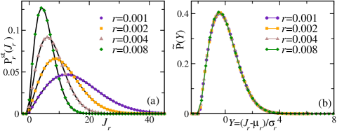
The stationary distribution has some interesting features which are visible from Fig. 9(a). First, it is apparent that $P_{r}^{\text{st}}(J_{r})$ is vanishingly small for negative values of $J_{r}.$ This can be understood in the following way. Let us recall that, at any time, the total current is nothing but the net number of particles hopping across the central bond since the last resetting event, i.e., after being brought to the configuration ${\mathcal{C}}_{0}$ where the left half of the lattice is filled-up. To produce a negative current, the number of particles crossing the central bond from left to right should be lower than that from right to left i.e., there should be a net flux of the particles to the left. Since, the particles are allowed to hop only to empty neighbouring sites, starting from the configuration ${\mathcal{C}}_{0},$ this is an extremely unlikely event and has a vanishingly small probability.

Secondly, it also appears that $P_{r}^{\text{st}}(J_{r})$ is strongly non-Gaussian which is manifest in the asymmetric behaviour of the two tails, as seen in Fig. 9(a). To characterize this asymmetry and the non-Gaussian nature quantitatively we look at the decay of $P_{r}^{\text{st}}(J_{r})$ at the two tails, namely, near $J_{r}=0$ and large $J_{r}.$ Near $J_{r}=0,$ for small values of $r,$ the behaviour is dominated by the $n=0$ term in Eq. (100). One can then use the asymptotic behaviour of $K_{\frac{3}{2}}(z)$ near $z=0$ to get

$$P_{r}^{\text{st}}(J_{r})\approx 2\pi r\left(J_{r}+1-\frac{1}{\sqrt{2}}\right)+\mathcal{O}(r^{2}).$$ (101)

Clearly, for small values of $r,$ the probability distribution of the total current $J_{r}$ decays linearly near $J_{r}=0.$

To determine how $P_{r}^{\text{st}}(J_{r})$ decays for large $J_{r}$ we use the asymptotic behaviour of $K_{\nu}(z);$ for large values of the argument $z,$ we have (see Ref. polylog , Eq. 10.40.2),

$$\lim_{z\to\infty}K_{\nu}(z)\approx\sqrt{\frac{\pi}{2z}}e^{-z}.$$ (102)

Using that in Eq. (100) and performing the sum over $n,$ we get,

$$P_{r}^{\text{st}}(J_{r})\approx 2\pi rJ_{r}e^{-\pi rJ_{r}^{2}}+\mathcal{O}(r^{2}).$$ (103)

Note that the above expression holds true to the leading order in $r,$ higher order corrections can be systematically calculated by including higher order terms in (102).

We conclude the discussion about $P_{r}^{\text{st}}(J_{r})$ with one final remark. From our numerical data, we observe a surprising collapse of the current distribution when plotted as a function of the scaled variable $Y=(J_{r}-\mu_{r})/\sigma_{r}$ where $\mu_{r}$ and $\sigma_{r}$ are, respectively, the mean and the variance of $J_{r}.$ The collapse is shown in Fig. 9(b) where the scaled distribution $\tilde{P}(Y)$ appears to be independent of $r$ as the curves corresponding to different values of $r$ from Fig. 9(a) fall on top of each other. To understand this collapse, let us look at $\tilde{P}(Y)$ predicted from Eqs. (103) and (101). Recalling that for small values of $r,$ $\mu_{r}\simeq\frac{1}{2\sqrt{r}}$ and $\sigma_{r}\simeq\sqrt{\frac{(4-\pi)}{4\pi r}},$ we get from Eq. (103),

$$\tilde{P}(Y) \approx \frac{1}{2}\bigg{(}\sqrt{\pi(4-\pi)}+(4-\pi)Y\bigg{)}e^{-\frac{1}{4}(\sqrt{\pi}+\sqrt{4-\pi}Y)^{2}}$$ (105)

$$\qquad+~{}\mathcal{O}(r^{3/2}).$$

Clearly, to the leading order in $r,$ $\tilde{P}(Y)$ calculated from Eq. (103) (corresponding to large values of $J_{r}$) is independent of $r,$ and is consistent with the scaling collapse observed in Fig. 9(b). On the other hand, it can be easily seen, that Eq.(101) does not lend itself to a similar form; $\tilde{P}(Y)$ derived from Eq.(101) depends explicitly on $r,$

$$\tilde{P}(Y) \approx \frac{1}{2}\sqrt{\pi(4-\pi)}\bigg{(}1+\sqrt{\frac{4-\pi}{\pi}}Y+(2-\sqrt{2})\sqrt{r}\bigg{)}$$ (107)

$$+\mathcal{O}(r^{3/2}).$$

Hence, while for large positive $J_{r}$ ($\gtrsim\mu_{r}+\sigma_{r}$), the distribution $\tilde{P}(Y)$ becomes independent of $r$, it is not the case in the $J_{r}\to 0$ limit. Indeed, as seen from Eq. (107), $\tilde{P}(Y)$ explicitly depends on $r.$ However, notice that the $r$-dependence in Eq. (107) comes in the form of an additional term proportional to $\sqrt{r},$ which is vanishingly small for $r\ll 1.$ This makes the expected mismatch in the collapse at the left tail in Fig. 9(b) practically invisible where an apparent collapse is also observed.

V Conclusion

In this article, we explore the effect of stochastic resetting on interacting many particle systems. To this end, we study the dynamical properties of a canonical set-up, namely, the symmetric exclusion process in the presence of stochastic resetting. The resetting is implemented by interrupting the dynamical evolution of the exclusion process with some rate $r$ and restarting it from a step-like configuration where all the particles are clustered together in the left-half of the system.

We find that the presence of resetting strongly affects the behaviour of the system. The key findings are as follows. First, in a finite size system, the density profile evolves to an inhomogeneous stationary profile in contrast to the flat profile in the absence of resetting. We have exactly calculated the full time-dependent density profile for arbitrary resetting rate $r.$ Secondly, we find that, in a thermodynamically large system the resetting mechanism drastically changes the $\sqrt{t}$ growth of the diffusive current to linear in $t$. We have explicitly computed the mean and variance of the diffusive current, the latter is also shown to have a linear growth in the long-time regime. Apart from the diffusive current, we also identify the another component of the current which arises due the resetting move and show that this resetting current is negative, with a linear temporal growth in magnitude. The moments of the total current, i.e., the sum of the diffusive and resetting current, are also calculated using the renewal approach.

We also have investigated the probability distribution of the diffusive current $J_{\text{d}},$ resetting current $J_{\text{reset}},$ as well the total current $J_{r}.$ We have found that that while the typical fluctuations of $J_{\text{d}}$ and $J_{\text{reset}}$ are Gaussian in nature, the distribution of $J_{r}$ is strictly non-Gaussian. The non-Gaussian nature is manifest in the asymmetric asymptotic behaviour of the distribution at the two tails, which we also demonstrate.

Our study opens up a new direction in the area of stochastic resetting and gives rise to a wide range of further questions. For example, it would be interesting to study the effect of stochastic resetting in other interacting particle systems, e.g., the asymmetric exclusion process, driven and equilibrium lattice gas models etc. Furthermore, it would also be interesting to study behavior of these interacting particle systems under various other resetting mechanisms like resetting at power-law times or time-dependent resetting etc.

Apart from these theoretical questions, the framework of stochastic resetting in exclusion processes can also be relevant in the context of certain biophysical systems. For example, stochastic motion of backtracked RNA polymerases can be modelled as an interacting many particle random walk on the DNA template, with RNA cleavage playing the role of resetting dynamics bio3 ; Lisica .
Similarly, motion of two-headed molecular motors such as kinesin and Myosin V moving on a polymeric track can be modelled as an energy driven hopping process in the presence of backward jumps (or resetting)Astumian . We believe that the formalism introduced in the present work will be useful in understanding such systems.

Appendix A Density profile of SEP in absence of resetting

In this section we present a brief account of the dynamical evolution of the density profile and current for ordinary SEP, starting from the step-like configuration $\mathcal{C}_{0}.$ In absence of resetting, the time evolution of the system is governed by the free Markov matrix ${\mathcal{L}}_{0}$ which yields, for the density profile,

$$\frac{\textrm{d}}{\textrm{d}t}\rho_{0}(x,t) = \rho_{0}(x+1,t)+\rho_{0}(x-1,t)-2\rho_{0}(x,t).\;\;$$ (108)

The corresponding Fourier components $\tilde{\rho}_{0}(n,t)$ evolve following,

$$\frac{\textrm{d}}{\textrm{d}t}\tilde{\rho}_{0}(n,t)=-\lambda_{n}\tilde{\rho}_{0}(n,t)$$ (109)

where, as before, $\lambda_{n}=2\left(1-\cos\frac{2\pi n}{L}\right),$ with $n=0,1,2,\dots L-1.$ The above equation is immediately solved to obtain,

$$\tilde{\rho}_{0}(n,t)=e^{-\lambda_{n}t}\tilde{\phi}(n).$$ (110)

where $\tilde{\phi}(n)$ corresponds to the initial profile $\phi(x).$ Note that $\lambda_{0}=0$ and hence $\tilde{\rho}_{0}(0,t)=\tilde{\phi}(0)=\frac{L}{2}$ does not evolve with time.

The spatial density profile is obtained by taking inverse Fourier transform of Eq. (110). In particular, for the step-like initial profile $\phi(x)=1-\Theta(x+1-\frac{L}{2})$ we have,

$$\rho_{0}(x,t)=\frac{1}{2}+\frac{1}{L}\sum_{n=1,3}^{L-1}e^{-i\frac{2\pi nx}{L}}\left(1+i\cot\frac{\pi n}{L}\right)e^{-\lambda_{n}t}~{}~{}\;\;$$ (111)

Appendix B Behaviour of current in absence of resetting

In the absence of resetting the only source of current in SEP is the hopping dynamics of the particles. The average instantaneous current across the initial step, i.e., across the central bond $\left(\frac{L}{2}-1,\frac{L}{2}\right)$ is given by,

$$\langle j_{0}(t)\rangle = \rho_{0}\left(\frac{L}{2}-1,t\right)-\rho_{0}\left(\frac{L}{2},t\right)$$ (112)

$$= \frac{2}{L}\sum_{n=1,3}^{L-1}e^{-\lambda_{n}t}$$ (113)

where we have used Eq. (111) to calculate the average densities at the sites $x=\frac{L}{2}-1$ and $x=\frac{L}{2}.$ Clearly, in the long-time limit $t\to\infty,$ the instantaneous current vanishes as the density profile becomes flat.

We are interested in the time-integrated current $J_{0}(t)=\int_{0}^{t}\textrm{d}s~{}j_{0}(s)$ which measures the net number of particles crossing the central bond towards right. The average time-integrated current is obtained by integrating Eq. (113),

$$\langle J_{0}(t)\rangle=\frac{2}{L}\sum_{n=1,3}^{L-1}\frac{1}{\lambda_{n}}(1-e^{-\lambda_{n}t}).$$ (114)

For any finite $L,$ the average time-integrated current $J_{0}(t)$ saturates to an $L$-dependent constant value in the long-time limit.

To understand the behaviour of a thermodynamically large system, one has to take the limit $L\to\infty$ first. In this case, the sum in Eq. (113) can be can be converted to an integral by denoting $q=2\pi n/L,$ and we have the mean instantaneous current,

$$\langle j_{0}(t)\rangle = \int_{0}^{2\pi}\frac{\textrm{d}q}{2\pi}~{}e^{-2(1-\cos q)t}$$

$$= e^{-2t}I_{0}(2t).$$

Here $I_{0}(x)$ is the Modified Bessel function of the first kind polylog (see Eq. 10.25.2 therein). In this limit, the average time-integrated current becomes,

$$\langle J_{0}(t)\rangle=e^{-2t}t[I_{0}(2t)+I_{1}(2t)].$$ (116)

For large values of the argument $x,$ both $I_{0}(x)$ and $I_{1}(x)$ have the same asymptotic behaviour (see polylog , Eq. 10.40.1 ),

$$\lim_{x\to\infty}I_{0,1}(2x)\sim\frac{e^{2x}}{2\sqrt{\pi x}}$$ (117)

which yields, in the long-time regime,

$$\langle J_{0}(t)\rangle\simeq\sqrt{\frac{t}{\pi}}.$$ (118)

This result has been obtained in Ref. Derrida1 , albeit using a different method. In fact, it has also been shown Derrida1 that, in the long-time regime, all the higher moments of $J_{0}$ show a similar behaviour. In particular, the variance is given by,

$$\langle J_{0}^{2}(t)\rangle-\langle J_{0}(t)\rangle^{2}\simeq\sqrt{\frac{t}{\pi}}\left(1-\frac{1}{\sqrt{2}}\right).$$ (119)

The above equation is used in Eq. (86) in the main text to calculate $\langle J_{r}^{2}\rangle.$

B.1 Probability Distribution of $J_{0}$

For ordinary SEP, the probability distribution of the time-integrated current $J_{0}$ was explored in Ref. Derrida1 . There the authors considered a scenario where, initially, each site to the left (respectively, right) of the origin ($x\leq 0$ and $x>0$ respectively) is occupied with probability $\rho_{a}$ (respectively $\rho_{b}$). It was shown that, for large $t,$ the moment generating function of the total particle flux $J_{0}(t)$ through the origin is given by,

$$\langle e^{\lambda J_{0}(t)}\rangle\sim e^{\sqrt{t}F(\omega)}$$ (120)

where $\omega=\rho_{a}(e^{\lambda}-1)+\rho_{b}(e^{-\lambda}-1)+\rho_{a}\rho_{b}(e^{\lambda}-1)$ and

$$F(\omega) = \frac{1}{\sqrt{\pi}}\sum_{n=1}^{\infty}\frac{(-1)^{n+1}\omega^{n}}{n^{3/2}}$$ (121)

$$\equiv -\frac{1}{\sqrt{\pi}}\text{PolyLog}_{3/2}(-\omega).$$ (122)

In our case, we have $\rho_{a}=1$ and $\rho_{b}=0$ which simplifies $\omega$ and in turn $F(\omega);$ we get $\omega=e^{\lambda}-1$ and

$$F(\lambda)=-\frac{1}{\sqrt{\pi}}\text{PolyLog}_{3/2}(1-e^{\lambda})$$ (123)

which is quoted in Eq. (49) in the main text.

It has been shown in Ref. Derrida1 that the corresponding probability distribution $P_{0}(J_{0},t),$ in the long-time limit, is of the form,

$$P_{0}(J_{0},t)\sim e^{\sqrt{t}G(J_{0}/\sqrt{t})}.$$ (124)

The large deviation function $G(q=J_{0}/\sqrt{t})$ is related to $F(\lambda)$ through a Legendre transform,

$$G(q) = \min_{\lambda}[F(\lambda)-\lambda q]$$ (125)

$$= F(\lambda^{*})-\lambda^{*}q,$$ (126)

where $\lambda^{*}$ corresponds to the minimum of the function $F(\lambda)-\lambda q$ and is obtained by solving $\frac{\textrm{d}F(\lambda)}{\textrm{d}\lambda}=q.$ It is easy to see that for small values of $q,$ $\lambda^{*}$ is also small. Hence, it is convenient to use the series expansion of $F(\lambda)$ near $\lambda=0$

$$F(\lambda)=\frac{\lambda}{\sqrt{\pi}}+\frac{\lambda^{2}}{2\sqrt{\pi}}\left(1-\frac{1}{\sqrt{2}}\right)+\mathcal{O}(\lambda^{3}),$$ (127)

to find $\lambda^{*}$ for small values of $q.$ Restricting ourselves to the quadratic order in $\lambda,$ we get $\lambda^{*}=\frac{(q\sqrt{\pi}-1)\sqrt{2}}{(\sqrt{2}-1)}.$ Substitution of this $\lambda^{*}$ in Eq. (126) yields,

$$G(q)=\frac{(q-\frac{1}{\sqrt{\pi}})^{2}}{\frac{2}{\sqrt{\pi}}(1-\frac{1}{\sqrt{2}})}$$ (128)

Using the above $G(q)$ in Eq. (124) results in a Gaussian form for the current distribution,

$$P_{0}(J_{0},t)=\frac{1}{\sqrt{2\pi\sigma_{0}^{2}(t)}}\exp{\bigg{(}-\frac{[J_{0}-\mu_{0}(t)]^{2}}{2\sigma^{2}_{0}(t)}\bigg{)}}$$ (129)

where the prefactor is just a normalization constant. Here, $\mu_{0}(t)=\sqrt{\frac{t}{\pi}}$ is nothing but the average hopping current $\langle J_{0}(t)\rangle$ and $\sigma_{0}^{2}(t)=\sqrt{\frac{t}{\pi}}\left(1-\frac{1}{\sqrt{2}}\right)$ is the variance [see Eq. (119)]. Note that, this Gaussian distribution is expected only in the long-time limit, as Eq. (124) holds true in this limit only.

Figure 10: (a) Plot of $P_{0}(J_{0},t)$ vs $J_{0}$ for different (large) values of $t.$ The symbols indicate the data obtained from numerical simulation of a system of size $L=1000,$ whereas the solid black lines correspond to the Gaussian distribution (see Eq. (129)). (b) The same data plotted as function of $(J_{0}-\mu_{0}(t))/\sigma_{0}(t);$ the solid line indicates the standard normal distribution.

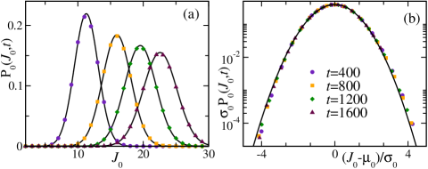
Figure 10 (a) shows a comparison of $P_{0}(J_{0},t)$ obtained from numerical simulations (symbols) with the that predicted from Eq. (129) (solid lines) for different (large) values of $t.$ Fig. 10 (b) shows the same data but plotted against the scaled variable $y=\frac{J_{0}-\mu_{0}(t)}{\sigma_{0}(t)};$ the solid line corresponds to the standard normal distribution $\frac{1}{\sqrt{2\pi}}e^{-y^{2}/2}.$ The numerical data shows a very good match with the predicted Gaussian curve for typical values of $J_{0},$ there are deviations only at the regime $|y|\gg 1$ which are visible only at a logarithmic scale. The large deviation function calculated in Ref Derrida1 describes the distribution for these atypical values. However, as shown in Sec. IV.3, for our purposes it suffices to consider the typical fluctuations and we use the Gaussian distribution (129) to calculate the distribution of the diffusive current $J_{\text{d}}$ in presence of resetting.

References

- (1) O. Bénichou, C. Loverdo, M. Moreau, and R. Voituriez, Rev. Mod. Phys. 83, 81 (2011).
- (2) A. Chechkin and I. M. Sokolov Phys. Rev. Lett. 121, 050601 (2018).
- (3) A. Pal and S. Reuveni, Phys. Rev. Lett. 118, 030603 (2017).
- (4) A. Pal, Ł. Kuśmierz, S. Reuveni, arXiv:1906.06987.
- (5) S. C. Manrubia and D. H. Zanette Phys. Rev. E 59, 4945 (1999).
- (6) P. Visco, R. J. Allen, S. N. Majundar, and M. R. Evans, Biophys. J. 98, 1099 (2010).
- (7) T. Rotbart, S. Reuveni and M. Urbakh, Phys. Rev. E 92, 060101(R) (2015).
- (8) S. Reuveni, M. Urbakh, and J. Klafter, Proc. Natl. Acad. Sci. 111, 4391 (2014).
- (9) A. Montanari and R. Zecchina, Phys. Rev. Lett. 88, 178701 (2002).
- (10) L. Lovasz, in Combinatronics, Vol. 2, p. 1, (Bolyai Society for Mathematical Studies, Budapest), 1996.
- (11) D. Sornette, Phys. Rep. 378, 1 (2003); D. Sornette, Why Stock Markets Crash (Princeton, NJ: Princeton University Press), 2017.
- (12) E. Kussell and S. Leiber, Science 309, 2075 (2005).
- (13) E. Kussell, R. Kishony, N. Q. Balaban and S. Leiber, Genetics 169, 1807 (2005).
- (14) E. Roldán, A. Lisica, D. Sánchez-Taltavull, and S. W. Grill, Phys. Rev. E 93, 062411 (2016).
- (15) M. R. Evans and S. N. Majumdar, Phys. Rev. Lett. 106, 160601 (2011).
- (16) M. R. Evans and S. N. Majumdar, J. Phys. A: Math. Theor. 44, 435001 (2011).
- (17) M. R. Evans, S. N. Majumdar, and K. Mallick, J. Phys. A: Math. Theor. 46, 185001 (2013).
- (18) J. Whitehouse, M. R. Evans, and S. N. Majumdar, Phys. Rev. E 87, 022118 (2013).
- (19) M. R. Evans and S. N. Majumdar, J. Phys. A: Math. Theor. 47, 285001 (2014).
- (20) V. Méndez and D. Campos, Physical Review E 93, 022106 (2016).
- (21) A. Masó-Puigdellosas, D. Campos, and V. Méndez, Physical Review E 99, 012141 (2019).
- (22) D. Gupta, J. Stat. Mech., 033212 (2019).
- (23) A. Pal, R. Chatterjee, S. Reuveni, and A. Kundu, J. Phys. A 52, 264002 (2019).
- (24) A. Pal, Phys. Rev. E 91, 012113 (2015).
- (25) S. Ahmad, I. Nayak, A. Bansal, A. Nandi, and D. Das, Phys. Rev. E 99, 022130 (2019).
- (26) A. Chatterjee, C. Christou, and A. Schadschneider, Phys. Rev. E 97, 062106 (2018).
- (27) A. Pal and V. V. Prasad, Phys. Rev. E 99, 032123 (2019)
- (28) M. Basu, P. K. Mohanty, Europhys. Lett., 90, 50005 (2010).
- (29) D. Boyer and C. Solis-Salas, Phys. Rev. Lett. 112, 240601 (2014).
- (30) S. N. Majumdar, S. Sabhapandit, and G. Schehr, Phys. Rev. E 92, 052126 (2015).
- (31) Ł. Kuśmierz, S. N. Majumdar, S. Sabhapandit, and G. Schehr, Phys. Rev. Lett. 113, 220602 (2014).
- (32) X. Durang, M. Henkel, and H. Park, J. Phys. A: Math. Theor. 47, 045002 (2014).
- (33) J. Masoliver, Phys. Rev. E 99, 012121 (2019).
- (34) M. R. Evans, S. N. Majumdar, J. Phys. A: Math. Theor. 51, 475003 (2018).
- (35) C. Maes and T. Thiery, J. Phys. A: Math. Theor. 50, 415001 (2017).
- (36) U. Bhat, C. De Bacco, and S. Redner J. Stat. Mech., 083401 (2016).
- (37) E. Roldán, S. Gupta, Phys. Rev. E 96, 022130 (2017).
- (38) A. Pal, A. Kundu, and M. R. Evans J. Phys. A: Math. Theor. 49, 225001 (2016).
- (39) V. P. Shkilev, Phys. Rev. E 96, 012126 (2017).
- (40) M. R. Evans and S. N. Majumdar, J. Phys. A: Math. Theor. 52, 01LT01 (2019).
- (41) A. Masó-Puigdellosas, D. Campos and V. Méndez, J. Stat. Mech., 033201 (2019).
- (42) A. Nagar and S. Gupta, Phys. Rev. E 93, 060102 (2016).
- (43) S. Eule and J. J. Metzger, New J. Phys. 18, 033006 (2016).
- (44) A. S. Bodrova, A. V. Chechkin, I. M. Sokolov, Phys. Rev. E 100, 012120 (2019); Phys. Rev. E 100, 012119 (2019).
- (45) R. Falcao and M. R. Evans, J. Stat. Mech., 023204 (2017).
- (46) S. Gupta, S. N. Majumdar, and G. Schehr, Phys. Rev. Lett. 112, 220601 (2014).
- (47) S. Gupta and A. Nagar J. Phys. A: Math. Theor. 49, 445001 (2016).
- (48) B. Mukherjee, K. Sengupta, and S. N. Majumdar, Phys. Rev. B98, 104309 (2018).
- (49) T. T. da Silva and M. D. Fragoso, J. Phys. A: Math. Theor. 51, 505002 (2018).
- (50) T. Liggett, Interacting Particle Systems, Springer-Verlag, Berlin (1985).
- (51) F. Spitzer, Adv. in Math. 5, 256 (1970).
- (52) B. Derrida, A. Gerschenfeld, J. Stat. Phys. 136: 1 (2009).
- (53) B. Derrida, B. Douçot, and P. E. Roche, J. Stat. Phys. 115 (2004).
-
(54)
NIST Digital Library of Mathematical Functions. F. W. J. Olver, A. B. Olde Daalhuis, D. W. Lozier, B. I. Schneider, R. F. Boisvert, C. W. Clark, B. R. Miller, and B. V. Saunders, eds.
- (55) A. Lisica, C. Engel, M. Jahnel, E. Roldán, E. A. Galburt, P. Cramer, and S. W. Grill, Proc. Nat. Ac. Sc. 113, 2946 (2016).
- (56) R. D. Astumian, Biophys. J. 98, 2401 (2010).