\WarningFilter

captionUnsupported document class

Learning Orthogonal Projections in Linear Bandits

Qiyu Kang, and Wee Peng Tay, This research is supported in part by the Singapore Ministry of Education Academic Research Fund Tier 2 grant MOE2018-T2-2-019.The authors are with the School of Electrical and Electronic Engineering, Nanyang Technological University, Singapore. Email: kang0080@e.ntu.edu.sg, wptay@ntu.edu.sg.
Abstract

In a linear stochastic bandit model, each arm is a vector in an Euclidean space and the observed return at each time step is an unknown linear function of the chosen arm at that time step. In this paper, we investigate the problem of learning the best arm in a linear stochastic bandit model, where each arm’s expected reward is an unknown linear function of the projection of the arm onto a subspace. We call this the projection reward. Unlike the classical linear bandit problem in which the observed return corresponds to the reward, the projection reward at each time step is unobservable. Such a model is useful in recommendation applications where the observed return includes corruption by each individual’s biases, which we wish to exclude in the learned model. In the case where there are finitely many arms, we develop a strategy to achieve O(|𝔻|logn)𝑂𝔻𝑛O(|\mathbb{D}|\log n) regret, where n𝑛n is the number of time steps and |𝔻|𝔻|\mathbb{D}| is the number of arms. In the case where each arm is chosen from an infinite compact set, our strategy achieves O(n2/3(logn)1/2)𝑂superscript𝑛23superscript𝑛12O(n^{2/3}(\log{n})^{1/2}) regret. Experiments verify the efficiency of our strategy.

Index Terms:
Linear bandit, multi-armed bandit, orthogonal projection, discrimination aware

I Introduction

Multi-armed bandit (MAB) problems, introduced by Robbins [1] model the exploration and exploitation trade-off of sequential decision making under uncertainty. In its most basic paradigm, at each time step, the decision maker is given d𝑑d decisions or arms from which he is supposed to select one, and as a response, he observes a stochastic reward after each decision-making. The arm chosen at each time step is based on the information gathered at all the previous time steps. Therefore, in order to maximize the expected cumulative reward, exploitation of the current empirically best arm and exploration of less frequently chosen arms should be balanced carefully. Stochastic independence of rewards is assumed for different arms in some works like [2, 3, 4, 5, 6, 7, 8, 9, 10]. In other works like [11, 12, 13, 14, 15], reward dependence between arms is assumed, which allows the decision maker to gather information for more than one arm at each time step. One such specific assumption is that arms are vectors containing numeric elements, and the expected reward of choosing each arm is an inner product of the arm vector with an unknown parameter vector [16, 17, 14, 15]. In [14, 15], the authors proposed effective strategies that balance exploration and exploitation based on the optimism-in-the-face-of-uncertainty principle. This principle maintains a high probability confidence set for the estimated parameter vector, and at each time step, the decision maker chooses an arm and a parameter vector from the decision set and the confidence set respectively, so that their inner product is maximized. Note that the independent d𝑑d-armed bandit problem can be viewed as a special case of the general linear stochastic bandit problem, where the set of d𝑑d available decisions serves as a standard orthonormal basis of dsuperscript𝑑\mathbb{R}^{d}[14].

The linear stochastic bandit model has been successfully applied to some real-world problems like personalized news article recommendation [18], advertisement selection [19], and information retrieval [20]. For example, in news recommendation applications, typical features, including the news’ topic categories, the users’ race, gender, location, etc., can be treated as components in each arm or decision vector, while the users’ clicks are the rewards. A plausible recommendation scheme is to get as many clicks as possible. Another application is in sequential clinical trials [21, 22, 23] whose aims are to balance the correct identification of the best treatment (exploration) and the effectiveness of the treatment during the trials (exploitation). The classical sequential clinical trials containing d𝑑d different drugs can be modeled as an independent d𝑑d-armed bandit problem. However, this may be impractical as treatments may utilize multiple drugs simultaneously. A more feasible and general way is to model the treatment decision as a set of mixed drugs instead. An arm corresponds to a mixed drugs treatment with specific dosages of each kind. The reward at each time step is the curative efficacy after applying the mixed drug treatment to a patient at each trial.

However, in some scenarios, the decision maker is more interested in some criterion other than maximizing the cumulative reward in the standard linear stochastic bandit model. One example is a discrimination-aware movie recommendation system. To avoid racially discriminatory recommendations, a user’s race should not play any role in the recommendation system. However, the observed reward (number of clicks) may be biased by racial factors. A black user may have a history of following a particular black actor, but it does not mean that he or she should always be recommended movies with black actors. For example, Netflix last year angered black subscribers with targeted posters containing black actors no matter how minor their roles in the film are [24]. In principle, to avoid discrimination, protected or sensitive attributes such as race or gender should not be included in recommendation algorithms. Nonetheless, discarding such attributes directly and modeling the reward as a linear function of the other unprotected attributes may introduce system bias during the learning process. In another example, some clinical trials seek to maximize the curative effect on one disease of a mixed drugs treatment, while at the same time the patients who have this disease may concurrently have another disease. These patients need to take other drugs that have a positive or negative impact on the targeted disease. One typical example is the treatment of hypertension in chronic kidney disease. Hypertension is present in more than 80%percent8080\% of the patients with chronic kidney disease, and drugs like ACEi and ARB targeted for reducing proteinuria may also have an effect on blood pressure[25]. To study the effect of a mixed drug treatment targeted for controlling hypertension, the decision maker is supposed to discount the impact of drugs like ACEi and ARB in the decision process.

In this paper, we propose a linear stochastic bandit formulation that maximizes the (expected) cumulative reward over a subspace of decision attributes, based on the reward observed for the full space. Specifically, each arm is projected orthogonally onto a target subspace 𝕌𝕌\mathbb{U}. The reward is then decomposed into two components, one of which is due to 𝕌𝕌\mathbb{U}, and the other is due to 𝕌superscript𝕌perpendicular-to\mathbb{U}^{\perp}. We call the first component the projection reward and the second component the corruption. We develop a strategy that achieves111For non-negative functions f(n)𝑓𝑛f(n) and g(n)𝑔𝑛g(n), we write f(n)=O(g(n))𝑓𝑛𝑂𝑔𝑛f(n)=O(g(n)) if lim supnf(n)/g(n)<subscriptlimit-supremum𝑛𝑓𝑛𝑔𝑛\limsup_{n\to\infty}f(n)/g(n)<\infty, f(n)=o(g(n))𝑓𝑛𝑜𝑔𝑛f(n)=o(g(n)) if limnf(n)/g(n)=0subscript𝑛𝑓𝑛𝑔𝑛0\lim_{n\to\infty}f(n)/g(n)=0, and f(n)=Θ(g(n))𝑓𝑛Θ𝑔𝑛f(n)=\Theta(g(n)) if 0<lim infnf(n)/g(n)lim supnf(n)/g(n)<0subscriptlimit-infimum𝑛𝑓𝑛𝑔𝑛subscriptlimit-supremum𝑛𝑓𝑛𝑔𝑛0<\liminf_{n\to\infty}f(n)/g(n)\leq\limsup_{n\to\infty}f(n)/g(n)<\infty. O(|𝔻|logn)𝑂𝔻𝑛O(|\mathbb{D}|\log n) cumulative projection regret when there are finitely many |𝔻|𝔻|\mathbb{D}| arms and where n𝑛n is the number of time steps. In the case where the arms are drawn from an infinite compact set, we achieve a cumulative projection regret of O(n2/3(logn)1/2)𝑂superscript𝑛23superscript𝑛12O(n^{2/3}(\log{n})^{1/2}). Here, the projection regret at each time step is defined as the difference between the current expected projection reward of making one decision and the oracle best expected projection reward. This algorithm is based on the ϵtsubscriptitalic-ϵ𝑡\epsilon_{t}-greedy policy [2], which is a simple and well-known algorithm for the standard finite multi-armed bandit problem.

I-A Related Work

Two categories of work are related to our problem of interest: 1) the linear stochastic bandit model; and 2) the multi-objective Pareto bandit problem.

In the linear stochastic bandit model, the decision maker predicts the reward of an arm in dsuperscript𝑑\mathbb{R}^{d} based on the given context vector of this decision. In [26], the author proposed an algorithm based on least squares estimation and high probability confidence bounds, and showed that it has O(dnlog3/2(n|𝔻|))𝑂𝑑𝑛superscript32𝑛𝔻O(\sqrt{dn}\log^{3/2}(n|\mathbb{D}|)) regret upper bound for the case of finitely many decisions, where |𝔻|𝔻|\mathbb{D}| is the number of arms. The work [22] extended [26] to the problem with an arbitrary compact set of arms and presented a policy with O(dnlog3/2n)𝑂𝑑𝑛superscript32𝑛O(d\sqrt{n}\log^{3/2}n) regret upper bound. References [14, 15] further improved the regret upper bound using smaller confidence sets established using martingale techniques. In [27], the authors proposed a linear bandit formulation with hidden features where the reward of choosing one decision is the sum of two components, one of which is a linear function of the observable features, and the other is a linear function of the unobservable features. They applied a upper confidence bound (UCB)-type linear bandit policy with a coordinate descent [28, 29] algorithm in which estimating the hidden features and the unknown coefficients jointly over time is achieved. Our work is different from the above-mentioned papers in that we seek to maximize only the cumulative projection reward rather than the reward observed for the full space. Furthermore, the projection reward is formed by projecting both the decision arm and context vectors into a subspace.

In the stochastic multi-objective multi-armed bandit (MOMAB) problem [30, 31, 32, 33], the reward of making one decision is a vector rather than the scalar reward in the standard multi-armed bandit problem. Because of the possible conflicting objectives, a set of Pareto optimal arms [31] [34] is considered in the MOMAB problem instead of a single best arm. Scalarization techniques can be used to transform a MOMAB problem to a single objective MAB, and an arm belonging to the Pareto optimal set is regarded as a best arm in a particular scalarization function. In our work, we consider the decomposition of the reward where the decomposition is similar to a two-objective MAB applied with a linear scalarization function [31]. However, the difference between our model and MOMAB with linear scalarization is that we can only observe the sum of the (desired) projection reward and (undesired) corruption at each time step rather than a reward vector consisting of the two components as in MOMAB. Furthermore, our objective is to minimize the cumulative projection regret rather than minimizing the three types of regret defined in [31].

I-B Our Contributions

In this paper, we study the orthogonal projection problem in linear bandits, where our aim is to maximize the expected projection reward, which is an unknown linear function of a projection of the chosen arm onto a target subspace 𝕌d𝕌superscript𝑑\mathbb{U}\subseteq\mathbb{R}^{d}. In the case where there are finitely many arms, we develop a strategy to achieve O(|𝔻|logn)𝑂𝔻𝑛O(|\mathbb{D}|\log n) cumulative projection regret, where n𝑛n is the number of time steps and |𝔻|𝔻|\mathbb{D}| is the number of arms. In the case where the arm is chosen from an infinite compact set, our strategy achieves O(n2/3(logn)1/2)𝑂superscript𝑛23superscript𝑛12O(n^{2/3}(\log{n})^{1/2}) cumulative projection regret.

In the linear stochastic bandit literature, the best cumulative regret upper bound for the case of a compact decision set is O(dnpolylog(n))𝑂𝑑𝑛polylog𝑛O(d\sqrt{n}\,\text{polylog}(n)) [14, 15], where polylog(n)polylog𝑛\text{polylog}(n) means a polynomial in logn𝑛\log n. If a further smoothness assumption same as that in [15] is made, we show that it is possible to achieve the O(dn)𝑂𝑑𝑛O(d\sqrt{n}) projection regret upper bound in our problem formulation. However, the existence of a policy with O(dnpolylog(n))𝑂𝑑𝑛polylog𝑛O(d\sqrt{n}\,\text{polylog}(n)) cumulative projection regret for the general compact decision set remains an open question for our problem. We verify our proposed policies on both synthetic simulations and experiments on a wine quality dataset [35].

The rest of this paper is organized as follows. In Section II, we present our system model and assumptions. In Section III, we introduce our strategies and prove that they achieve sublinear cumulative projection regret. In Section IV, we present simulations and experiments to verify the performance of our strategies. Section V concludes the paper.

Notations: We use Ecsuperscript𝐸𝑐E^{c} to denote the complement of the event E𝐸E. The indicator function 𝟏A(ω)=1subscript1𝐴𝜔1{\bf 1}_{A}(\omega)=1 if and only if ωA𝜔𝐴\omega\in A. 𝐈𝐈\mathbf{I} is the identity matrix. For 𝐱,𝐲d𝐱𝐲superscript𝑑\mathbf{x},\mathbf{y}\in\mathbb{R}^{d}, let 𝐱superscript𝐱\mathbf{x}^{\intercal} be the transpose of 𝐱𝐱\mathbf{x} , and 𝐱,𝐲=𝐱𝐲𝐱𝐲superscript𝐱𝐲{\left\langle{\mathbf{x}},\,{\mathbf{y}}\right\rangle}=\mathbf{x}^{\intercal}\mathbf{y}. We use 𝐱2subscriptnorm𝐱2\|\mathbf{x}\|_{2} to denote the L2subscript𝐿2L_{2}-norm 𝐱,𝐱𝐱𝐱\sqrt{{\left\langle{\mathbf{x}},\,{\mathbf{x}}\right\rangle}} and 𝐱𝐀subscriptnorm𝐱𝐀\|\mathbf{x}\|_{\mathbf{A}} to denote the weighted L2subscript𝐿2L_{2}-norm 𝐱,𝐀𝐱𝐱𝐀𝐱\sqrt{{\left\langle{\mathbf{x}},\,{\mathbf{A}\mathbf{x}}\right\rangle}} for any 𝐀d×d𝐀superscript𝑑𝑑\mathbf{A}\in\mathbb{R}^{d\times d} is a positive definite matrix. We use 𝒰(a,b)𝒰𝑎𝑏\mathcal{U}(a,b) to denote the continuous uniform distribution whose density function has support [a,b]𝑎𝑏[a,b], and 𝒩(0,ϑ2)𝒩0superscriptitalic-ϑ2\mathcal{N}(0,\vartheta^{2}) to denote the Gaussian distribution with variance ϑ2superscriptitalic-ϑ2\vartheta^{2} and mean 00.

II System Model

Let 𝔻d𝔻superscript𝑑\mathbb{D}\subseteq\mathbb{R}^{d} be a compact set of decisions or arms from which the decision maker has to choose an arm Xtsubscript𝑋𝑡X_{t} at each time step t𝑡t. The observed return rtsubscript𝑟𝑡r_{t} after choosing Xtsubscript𝑋𝑡X_{t} is given by

rt=Xt,𝜽+ηt,subscript𝑟𝑡subscript𝑋𝑡𝜽subscript𝜂𝑡\displaystyle r_{t}={\left\langle{X_{t}},\,{\bm{\theta}}\right\rangle}+\eta_{t}, (1)

where 𝜽d𝜽superscript𝑑\bm{\theta}\in\mathbb{R}^{d} is a fixed but unknown parameter and ηtsubscript𝜂𝑡\eta_{t} is a zero mean independent and identically distributed (i.i.d.) random noise.

In the standard linear bandit problem, the performance of a policy is measured by the difference between the decision maker’s cumulative reward and the cumulative reward achieved by the oracle policy with knowledge of 𝜽𝜽\bm{\theta}. Formally, the goal of the decision maker is to minimize the cumulative regret over n𝑛n time steps defined by

R(n)=t=1n(X,𝜽𝔼[Xt,𝜽]),𝑅𝑛superscriptsubscript𝑡1𝑛superscript𝑋𝜽𝔼delimited-[]subscript𝑋𝑡𝜽\displaystyle R(n)=\sum_{t=1}^{n}\big{(}{\left\langle{X^{*}},\,{\bm{\theta}}\right\rangle}-\mathbb{E}\left[{{\left\langle{X_{t}},\,{\bm{\theta}}\right\rangle}}\right]\big{)}, (2)

where X=argmax𝐱𝔻𝐱,𝜽superscript𝑋subscriptargmax𝐱𝔻𝐱𝜽X^{*}=\operatorname*{arg\,max}_{\mathbf{x}\in\mathbb{D}}{\left\langle{\mathbf{x}},\,{\bm{\theta}}\right\rangle} is the optimal arm in the standard linear bandit problem.

In our orthogonal projection linear bandit model, we consider a decomposition of the observed return into two components. Let 𝕌𝕌\mathbb{U}, whose dimension is not more than d𝑑d, be a subspace of the Euclidean vector space dsuperscript𝑑\mathbb{R}^{d}. Let 𝕌={𝐪d:𝐪,𝐩=0,𝐩𝕌}superscript𝕌perpendicular-toconditional-set𝐪superscript𝑑formulae-sequence𝐪𝐩0for-all𝐩𝕌\mathbb{U}^{\perp}=\{\mathbf{q}\in\mathbb{R}^{d}:{\left\langle{\mathbf{q}},\,{\mathbf{p}}\right\rangle}=0,\forall\mathbf{p}\in\mathbb{U}\} be the orthogonal complement of 𝕌𝕌\mathbb{U}. It is a standard result [36] that d=𝕌𝕌superscript𝑑direct-sum𝕌superscript𝕌perpendicular-to\mathbb{R}^{d}=\mathbb{U}\oplus\mathbb{U}^{\perp}, and each 𝐰d𝐰superscript𝑑\mathbf{w}\in\mathbb{R}^{d} can be written uniquely as a sum 𝐩+𝐪𝐩𝐪\mathbf{p}+\mathbf{q}, where 𝐩𝕌𝐩𝕌\mathbf{p}\in\mathbb{U} and 𝐪𝕌𝐪superscript𝕌perpendicular-to\mathbf{q}\in\mathbb{U}^{\perp}. We define the linear orthogonal projection operator as P𝕌:d𝕌:subscript𝑃𝕌maps-tosuperscript𝑑𝕌P_{\mathbb{U}}:\mathbb{R}^{d}\mapsto\mathbb{U} such that P𝕌(𝐰)=𝐩subscript𝑃𝕌𝐰𝐩P_{\mathbb{U}}(\mathbf{w})=\mathbf{p}. The operator P𝕌subscript𝑃𝕌P_{\mathbb{U}} can be represented by a d×d𝑑𝑑d\times d matrix whose rank is the dimension of 𝕌𝕌\mathbb{U}. The expected observed return can therefore be decomposed as

Xt,𝜽subscript𝑋𝑡𝜽\displaystyle{\left\langle{X_{t}},\,{\bm{\theta}}\right\rangle} =P𝕌(Xt)+P𝕌(Xt),P𝕌(𝜽)+P𝕌(𝜽)absentsubscript𝑃𝕌subscript𝑋𝑡subscript𝑃superscript𝕌perpendicular-tosubscript𝑋𝑡subscript𝑃𝕌𝜽subscript𝑃superscript𝕌perpendicular-to𝜽\displaystyle={\left\langle{P_{\mathbb{U}}(X_{t})+P_{\mathbb{U}^{\perp}}(X_{t})},\,{P_{\mathbb{U}}(\bm{\theta})+P_{\mathbb{U}^{\perp}}(\bm{\theta})}\right\rangle}
=P𝕌(Xt),P𝕌(𝜽)+P𝕌(Xt),P𝕌(𝜽).absentsubscript𝑃𝕌subscript𝑋𝑡subscript𝑃𝕌𝜽subscript𝑃superscript𝕌perpendicular-tosubscript𝑋𝑡subscript𝑃superscript𝕌perpendicular-to𝜽\displaystyle={\left\langle{P_{\mathbb{U}}(X_{t})},\,{P_{\mathbb{U}}(\bm{\theta})}\right\rangle}+{\left\langle{P_{\mathbb{U}^{\perp}}(X_{t})},\,{P_{\mathbb{U}^{\perp}}(\bm{\theta})}\right\rangle}. (3)

We call P𝕌(Xt),P𝕌(θ)subscript𝑃𝕌subscript𝑋𝑡subscript𝑃𝕌𝜃{\left\langle{P_{\mathbb{U}}(X_{t})},\,{P_{\mathbb{U}}(\theta)}\right\rangle} the projection reward on the subspace 𝕌𝕌\mathbb{U}, which is denoted by r𝕌,tsubscript𝑟𝕌𝑡r_{\mathbb{U},t}. The other part of the observed return, P𝕌(Xt),P𝕌(𝜽)subscript𝑃superscript𝕌perpendicular-tosubscript𝑋𝑡subscript𝑃superscript𝕌perpendicular-to𝜽{\left\langle{P_{\mathbb{U}^{\perp}}(X_{t})},\,{P_{\mathbb{U}^{\perp}}(\bm{\theta})}\right\rangle}, is called the corruption. Different from the standard linear bandit model, where the reward can be observed (with random perturbation), in our orthogonal projection linear bandit model, we do not directly observe the projection reward r𝕌,tsubscript𝑟𝕌𝑡r_{\mathbb{U},t}. Furthermore, the cumulative projection regret is defined as

R𝕌(n)=t=1n(P𝕌(X𝕌(𝜽)),P𝕌(𝜽)𝔼[P𝕌(Xt),P𝕌(𝜽)]),subscript𝑅𝕌𝑛superscriptsubscript𝑡1𝑛subscript𝑃𝕌superscriptsubscript𝑋𝕌𝜽subscript𝑃𝕌𝜽𝔼delimited-[]subscript𝑃𝕌subscript𝑋𝑡subscript𝑃𝕌𝜽\displaystyle R_{\mathbb{U}}(n)=\sum_{t=1}^{n}\big{(}{\left\langle{P_{\mathbb{U}}(X_{\mathbb{U}}^{*}(\bm{\theta}))},\,{P_{\mathbb{U}}(\bm{\theta})}\right\rangle}-\mathbb{E}\left[{{\left\langle{P_{\mathbb{U}}(X_{t})},\,{P_{\mathbb{U}}(\bm{\theta})}\right\rangle}}\right]\big{)}, (4)

where

X𝕌(𝜽)=argmax𝐱𝔻P𝕌(𝐱),P𝕌(𝜽)superscriptsubscript𝑋𝕌𝜽subscriptargmax𝐱𝔻subscript𝑃𝕌𝐱subscript𝑃𝕌𝜽\displaystyle X_{\mathbb{U}}^{*}(\bm{\theta})=\operatorname*{arg\,max}_{\mathbf{x}\in\mathbb{D}}{\left\langle{P_{\mathbb{U}}(\mathbf{x})},\,{P_{\mathbb{U}}(\bm{\theta})}\right\rangle} (5)

is the best projection arm. The objective in our model is to minimize the cumulative projection regret R𝕌(n)subscript𝑅𝕌𝑛R_{\mathbb{U}}(n) rather than the cumulative regret R(n)𝑅𝑛R(n), base on the observed returns r1,,rn1subscript𝑟1subscript𝑟𝑛1r_{1},\ldots,r_{n-1}.

For a concrete illustration, consider again the discrimination prevention problem in a movie recommendation system described in Section I. An arm is a movie to be recommended to a specific set of users and is represented by the features of the movie. The features include the movie genre, movie length, music types used, ages and races of the actors or actresses, etc. Suppose that each arm is a d𝑑d dimensional vector, where some of its elements like the ages and races may lead to discriminatory recommendations and are “protected”. To eliminate the effect of those features when performing the recommendations, the system should consider only the non-protected dimensions. In [37], the authors proposed to control the discrimination effect in a linear regression model, where P𝕌subscript𝑃𝕌P_{\mathbb{U}} in their formulation can also be viewed as a projection matrix.

We use span(𝔻)span𝔻\text{span}(\mathbb{D}) to denote the set of finite linear combinations of arms in 𝔻𝔻\mathbb{D}. In the ideal case, if at each time step t𝑡t the return rtsubscript𝑟𝑡r_{t} is available without the random noise ηtsubscript𝜂𝑡\eta_{t}, and if 𝔻𝔻\mathbb{D} is specified by linear inequality constraints, the problem then degenerates to a linear programming problem that finds 𝐱𝔻𝐱𝔻\mathbf{x}\in\mathbb{D} to maximize

P𝕌(𝐱),P𝕌(𝜽)subscript𝑃𝕌𝐱subscript𝑃𝕌𝜽\displaystyle{\left\langle{P_{\mathbb{U}}(\mathbf{x})},\,{P_{\mathbb{U}}(\bm{\theta})}\right\rangle}
=P𝕌(𝐱),𝜽absentsubscript𝑃𝕌𝐱𝜽\displaystyle={\left\langle{P_{\mathbb{U}}(\mathbf{x})},\,{\bm{\theta}}\right\rangle}
=P𝕌(𝐱),Pspan(𝔻)(𝜽)+Pspan(𝔻)(𝜽)absentsubscript𝑃𝕌𝐱subscript𝑃span𝔻𝜽subscript𝑃spansuperscript𝔻perpendicular-to𝜽\displaystyle={\left\langle{P_{\mathbb{U}}(\mathbf{x})},\,{P_{\text{span}(\mathbb{D})}(\bm{\theta})+P_{\text{span}(\mathbb{D})^{\perp}}(\bm{\theta})}\right\rangle}
=P𝕌(𝐱),Pspan(𝔻)(𝜽)+P𝕌(𝐱),Pspan(𝔻)(𝜽).absentsubscript𝑃𝕌𝐱subscript𝑃span𝔻𝜽subscript𝑃𝕌𝐱subscript𝑃spansuperscript𝔻perpendicular-to𝜽\displaystyle={\left\langle{P_{\mathbb{U}}(\mathbf{x})},\,{P_{\text{span}(\mathbb{D})}(\bm{\theta})}\right\rangle}+{\left\langle{P_{\mathbb{U}}(\mathbf{x})},\,{P_{\text{span}(\mathbb{D})^{\perp}}(\bm{\theta})}\right\rangle}. (6)

However, since Pspan(𝔻)(𝜽)subscript𝑃spansuperscript𝔻perpendicular-to𝜽P_{\text{span}(\mathbb{D})^{\perp}}(\bm{\theta}) is unobservable even in the ideal case, and argmax𝐱𝔻subscriptargmax𝐱𝔻\operatorname*{arg\,max}_{\mathbf{x}\in\mathbb{D}} P𝕌(𝐱),Pspan(𝔻)(𝜽)subscript𝑃𝕌𝐱subscript𝑃span𝔻𝜽{\left\langle{P_{\mathbb{U}}(\mathbf{x})},\,{P_{\text{span}(\mathbb{D})}(\bm{\theta})}\right\rangle} is not equal to X𝕌(𝜽)superscriptsubscript𝑋𝕌𝜽X_{\mathbb{U}}^{*}(\bm{\theta}) in 5 when P𝕌(𝐱),Pspan(𝔻)(𝜽)0subscript𝑃𝕌𝐱subscript𝑃spansuperscript𝔻perpendicular-to𝜽0{\left\langle{P_{\mathbb{U}}(\mathbf{x})},\,{P_{\text{span}(\mathbb{D})^{\perp}}(\bm{\theta})}\right\rangle}\neq 0, a linear cumulative projection regret is therefore inevitable in the worst case. In order to get a sublinear cumulative regret, further assumptions are required.

A possible assumption is P𝕌(𝐱),Pspan(𝔻)(𝜽)=0subscript𝑃𝕌𝐱subscript𝑃spansuperscript𝔻perpendicular-to𝜽0{\left\langle{P_{\mathbb{U}}(\mathbf{x})},\,{P_{\text{span}(\mathbb{D})^{\perp}}(\bm{\theta})}\right\rangle}=0 for all 𝐱𝐱\mathbf{x} and 𝜽𝜽\bm{\theta}. This is equivalent to saying 𝕌span(𝔻)𝕌span𝔻\mathbb{U}\subseteq\text{span}(\mathbb{D}). To see this, note that this assumption means that Pspan(𝔻)(𝜽)kernel(P𝕌)=P𝕌=P𝕌subscript𝑃spansuperscript𝔻perpendicular-to𝜽kernelsubscript𝑃𝕌superscriptsubscript𝑃𝕌perpendicular-tosubscript𝑃superscript𝕌perpendicular-toP_{\text{span}(\mathbb{D})^{\perp}}(\bm{\theta})\in\text{kernel}(P_{\mathbb{U}})=P_{\mathbb{U}}^{\perp}=P_{\mathbb{U}^{\perp}}. It follows that span(𝔻)𝕌spansuperscript𝔻perpendicular-tosuperscript𝕌perpendicular-to\text{span}(\mathbb{D})^{\perp}\subseteq\mathbb{U}^{\perp}, which is equivalent to 𝕌span(𝔻)𝕌span𝔻\mathbb{U}\subseteq\text{span}(\mathbb{D}). We make the following assumption throughout this paper.

Assumption 1.

We have 𝕌span(𝔻)𝕌span𝔻\mathbb{U}\subseteq\text{span}(\mathbb{D}), the dimension of span(𝔻)span𝔻\text{span}(\mathbb{D}) is k𝑘k, where dim(𝕌)kddimension𝕌𝑘𝑑\dim(\mathbb{U})\leq k\leq d, and P𝕌(𝛉)2>0subscriptnormsubscript𝑃𝕌𝛉20\|P_{\mathbb{U}}(\bm{\theta})\|_{2}>0. Furthermore, the decision maker has access to k𝑘k linearly independent arms in 𝔻𝔻\mathbb{D}.

We use 𝔻k𝔻subscript𝔻𝑘𝔻\mathbb{D}_{k}\subseteq\mathbb{D} to denote the set containing the k𝑘k linearly independent arms in Assumption 1. The condition P𝕌(𝜽)2>0subscriptnormsubscript𝑃𝕌𝜽20\|P_{\mathbb{U}}(\bm{\theta})\|_{2}>0 guarantees 𝜽𝕌𝜽superscript𝕌perpendicular-to\bm{\theta}\notin\mathbb{U}^{\perp}. We also make another assumption which is standard in the literature for the linear bandit problem.

Assumption 2.

We have 𝛉2Ssubscriptnorm𝛉2𝑆\|\bm{\theta}\|_{2}\leq S, and max𝐱𝔻𝐱2Zsubscript𝐱𝔻subscriptnorm𝐱2𝑍\max_{\mathbf{x}\in\mathbb{D}}\|\mathbf{x}\|_{2}\leq Z, where S𝑆S and Z𝑍Z are positive finite constants. The random variables ηtsubscript𝜂𝑡\eta_{t} are drawn i.i.d. from a zero-mean sub-Gaussian distribution with parameter ϑitalic-ϑ\vartheta, i.e., 𝔼[eξηt]eξ2ϑ2/2𝔼delimited-[]superscript𝑒𝜉subscript𝜂𝑡superscript𝑒superscript𝜉2superscriptitalic-ϑ22\mathbb{E}\left[{e^{\xi\eta_{t}}}\right]\leq e^{\xi^{2}\vartheta^{2}/2} for all ξ𝜉\xi\in\mathbb{R}.

III Strategies and Regret Analysis

III-A Greedy Projection Strategy

The decision set 𝔻𝔻\mathbb{D} may contain finitely or infinitely many arms. In this section, we present a strategy with two settings, the first is applicable for the finite-arm case, and the other is applicable for the infinite-arm case. In the following, we use 𝜽^tsubscript^𝜽𝑡\hat{\bm{\theta}}_{t} to denote the L2subscript𝐿2L_{2} regularized least square estimate of 𝜽𝜽\bm{\theta} with parameter λ>0𝜆0\lambda>0, after the decision making at time step t𝑡t:

𝜽^t=𝐕t1i=1triXi,subscript^𝜽𝑡superscriptsubscript𝐕𝑡1superscriptsubscript𝑖1𝑡subscript𝑟𝑖subscript𝑋𝑖\displaystyle\hat{\bm{\theta}}_{t}=\mathbf{V}_{t}^{-1}\sum_{i=1}^{t}r_{i}X_{i}, (7)

where 𝐕t=λ𝐈+i=1tXiXisubscript𝐕𝑡𝜆𝐈superscriptsubscript𝑖1𝑡subscript𝑋𝑖superscriptsubscript𝑋𝑖\mathbf{V}_{t}=\lambda\mathbf{I}+\sum_{i=1}^{t}X_{i}X_{i}^{\intercal}. We propose a Greedy projEctioN sTRategY (GENTRY) that accounts for the corruption in the observed return to achieve sublinear cumulative projection regret. GENTRY is based on the ϵtsubscriptitalic-ϵ𝑡\epsilon_{t}-greedy policy [2], which is a simple and well-known algorithm for the standard finite multi-armed bandit problem. At each time step t𝑡t, the ϵtsubscriptitalic-ϵ𝑡\epsilon_{t}-greedy policy chooses with probability 1ϵt1subscriptitalic-ϵ𝑡1-\epsilon_{t} the arm with the highest empirical average reward, and with probability ϵtsubscriptitalic-ϵ𝑡\epsilon_{t} a random arm. Since in our problem, we focus our attention on the projection reward, GENTRY chooses with probability 1ϵt1subscriptitalic-ϵ𝑡1-\epsilon_{t} the arm with the highest empirical average projection reward defined as:

r¯t1(𝐱)=P𝕌(𝐱),P𝕌(𝜽^t1),subscript¯𝑟𝑡1𝐱subscript𝑃𝕌𝐱subscript𝑃𝕌subscript^𝜽𝑡1\displaystyle\bar{r}_{t-1}(\mathbf{x})={\left\langle{P_{\mathbb{U}}(\mathbf{x})},\,{P_{\mathbb{U}}(\hat{\bm{\theta}}_{t-1})}\right\rangle}, (8)

for each arm 𝐱𝔻𝐱𝔻\mathbf{x}\in\mathbb{D}. Another difference is, at each time step t𝑡t, GENTRY chooses with probability ϵtsubscriptitalic-ϵ𝑡\epsilon_{t} a random arm from 𝔻ksubscript𝔻𝑘\mathbb{D}_{k} rather than 𝔻𝔻\mathbb{D}. We define two different settings of ϵtsubscriptitalic-ϵ𝑡\epsilon_{t} as follows:

ϵtf=min{1,αkt} and ϵti=min{1,αkt1/3},superscriptsubscriptitalic-ϵ𝑡𝑓1𝛼𝑘𝑡 and superscriptsubscriptitalic-ϵ𝑡𝑖1𝛼𝑘superscript𝑡13\displaystyle\epsilon_{t}^{f}=\min\left\{1,\frac{\alpha k}{t}\right\}\text{ and }\epsilon_{t}^{i}=\min\left\{1,\frac{\alpha k}{t^{1/3}}\right\}, (9)

to handle the finite- and infinite-arm cases, respectively. The hyperparameter α>0𝛼0\alpha>0 is a fixed positive constant. The GENTRY strategy is summarized in Algorithm 1.

Algorithm 1 GENTRY
0:  Set ϵtsubscriptitalic-ϵ𝑡\epsilon_{t} to ϵtfsuperscriptsubscriptitalic-ϵ𝑡𝑓\epsilon_{t}^{f} or ϵtisuperscriptsubscriptitalic-ϵ𝑡𝑖\epsilon_{t}^{i} according to whether the problem is finite-arm or infinite-arm. Set hyperparameters α>0𝛼0\alpha>0 and λ>0𝜆0\lambda>0.
1:  Set t=1𝑡1t=1.
2:  loop
3:     Set ϵtsubscriptitalic-ϵ𝑡\epsilon_{t} using 9.
4:     With probability 1ϵt1subscriptitalic-ϵ𝑡1-\epsilon_{t}, choose argmax𝐱𝔻r¯t1(𝐱)subscriptargmax𝐱𝔻subscript¯𝑟𝑡1𝐱\operatorname*{arg\,max}_{\mathbf{x}\in\mathbb{D}}\bar{r}_{t-1}(\mathbf{x}) and with probability ϵtsubscriptitalic-ϵ𝑡\epsilon_{t} choose a random arm from 𝔻ksubscript𝔻𝑘\mathbb{D}_{k}.
5:     Update r¯(𝐱t)¯𝑟subscript𝐱𝑡\bar{r}(\mathbf{x}_{t}) using 8.
6:     Set t=t+1𝑡𝑡1t=t+1.
7:  end loop

In the following theorems, we give a sufficient condition on the hyperparameter α𝛼\alpha for the strategy to achieve O(logn)𝑂𝑛O(\log n) for the finite-arm case. We also show that our infinite-arm strategy achieves O(n2/3(logn)1/2)𝑂superscript𝑛23superscript𝑛12O(n^{2/3}(\log n)^{1/2}) regret for the infinite-arm case. The empirical impact of α𝛼\alpha is further studied in Section IV. Parameter λ𝜆\lambda can be set as a moderate value like Z2superscript𝑍2Z^{2}.

III-B Regret Analysis

III-B1 Finitely Many Arms

Theorem 1.

Suppose Assumptions 1 and 2 hold, 𝔻𝔻\mathbb{D} contains finitely many arms,

α>max{24dZ2ϑ2min𝐱X𝕌Δ𝐱2δ𝔻k,10}𝛼24𝑑superscript𝑍2superscriptitalic-ϑ2subscript𝐱superscriptsubscript𝑋𝕌superscriptsubscriptΔ𝐱2subscript𝛿subscript𝔻𝑘10\displaystyle\alpha>\max\left\{\frac{24dZ^{2}\vartheta^{2}}{\min_{\mathbf{x}\neq X_{\mathbb{U}}^{*}}\Delta_{\mathbf{x}}^{2}\delta_{\mathbb{D}_{k}}},10\right\} (10)

where Δ𝐱=P𝕌(X𝕌(𝛉))P𝕌(𝐱),P𝕌(𝛉)subscriptΔ𝐱subscript𝑃𝕌superscriptsubscript𝑋𝕌𝛉subscript𝑃𝕌𝐱subscript𝑃𝕌𝛉\Delta_{\mathbf{x}}={\left\langle{P_{\mathbb{U}}(X_{\mathbb{U}}^{*}(\bm{\theta}))-P_{\mathbb{U}}(\mathbf{x})},\,{P_{\mathbb{U}}(\bm{\theta})}\right\rangle}, and δ𝔻ksubscript𝛿subscript𝔻𝑘\delta_{\mathbb{D}_{k}} is a constant that depends on 𝔻ksubscript𝔻𝑘\mathbb{D}_{k}. Then GENTRY has cumulative projection regret of order O(|𝔻|logn)𝑂𝔻𝑛O(|\mathbb{D}|\log n), where n𝑛n is the number of time steps and |𝔻|𝔻|\mathbb{D}| is the number of arms.

Theorem 1 shows that if we choose α𝛼\alpha to be sufficiently large, GENTRY achieves order optimal regret.

Proof:

For any arm 𝐱𝔻𝐱𝔻\mathbf{x}\in\mathbb{D}, let the random variable Nt(𝐱)subscript𝑁𝑡𝐱N_{t}(\mathbf{x}) denote the total number of time steps within the first t𝑡t time steps that the arm 𝐱𝐱\mathbf{x} was chosen, i.e., Nn(𝐱)=t=1n𝟏{Xt=𝐱}subscript𝑁𝑛𝐱superscriptsubscript𝑡1𝑛subscript1subscript𝑋𝑡𝐱N_{n}(\mathbf{x})=\sum_{t=1}^{n}{\bf 1}_{\left\{X_{t}=\mathbf{x}\right\}}. Since

𝔼[R𝕌(n)]𝔼delimited-[]subscript𝑅𝕌𝑛\displaystyle\mathbb{E}\left[{R_{\mathbb{U}}(n)}\right] =𝔼t=1n(P𝕌(X𝕌(𝜽)),P𝕌(𝜽)P𝕌(Xt),P𝕌(𝜽))absent𝔼superscriptsubscript𝑡1𝑛subscript𝑃𝕌superscriptsubscript𝑋𝕌𝜽subscript𝑃𝕌𝜽subscript𝑃𝕌subscript𝑋𝑡subscript𝑃𝕌𝜽\displaystyle=\mathbb{E}\sum_{t=1}^{n}\bigg{(}{\left\langle{P_{\mathbb{U}}(X_{\mathbb{U}}^{*}(\bm{\theta}))},\,{P_{\mathbb{U}}(\bm{\theta})}\right\rangle}-{\left\langle{P_{\mathbb{U}}(X_{t})},\,{P_{\mathbb{U}}(\bm{\theta})}\right\rangle}\bigg{)}
=𝐱𝔻𝔼[Nn(𝐱)]Δ𝐱absentsubscript𝐱𝔻𝔼delimited-[]subscript𝑁𝑛𝐱subscriptΔ𝐱\displaystyle=\sum_{\mathbf{x}\in\mathbb{D}}\mathbb{E}\left[{N_{n}(\mathbf{x})}\right]\Delta_{\mathbf{x}}
=𝐱𝔻Δ𝐱t=1n(Xt=𝐱),absentsubscript𝐱𝔻subscriptΔ𝐱superscriptsubscript𝑡1𝑛subscript𝑋𝑡𝐱\displaystyle=\sum_{\mathbf{x}\in\mathbb{D}}\Delta_{\mathbf{x}}\sum_{t=1}^{n}\mathbb{P}\left({X_{t}=\mathbf{x}}\right), (11)

where Δ𝐱=P𝕌(X𝕌(𝜽))P𝕌(𝐱),P𝕌(𝜽)subscriptΔ𝐱subscript𝑃𝕌superscriptsubscript𝑋𝕌𝜽subscript𝑃𝕌𝐱subscript𝑃𝕌𝜽\Delta_{\mathbf{x}}={\left\langle{P_{\mathbb{U}}(X_{\mathbb{U}}^{*}(\bm{\theta}))-P_{\mathbb{U}}(\mathbf{x})},\,{P_{\mathbb{U}}(\bm{\theta})}\right\rangle} is the projection regret of arm 𝐱𝐱\mathbf{x}, it is sufficient to show that the probability (Xt=𝐱)=O(t1)subscript𝑋𝑡𝐱𝑂superscript𝑡1\mathbb{P}\left({X_{t}=\mathbf{x}}\right)=O(t^{-1}) for all suboptimal 𝐱𝔻\{X𝕌}𝐱\𝔻superscriptsubscript𝑋𝕌\mathbf{x}\in\mathbb{D}\backslash\{X_{\mathbb{U}}^{*}\}. We have

(Xt=𝐱)ϵtk+(1ϵt)(r¯t1(𝐱)r¯t1(X𝕌(𝜽))),subscript𝑋𝑡𝐱subscriptitalic-ϵ𝑡𝑘1subscriptitalic-ϵ𝑡subscript¯𝑟𝑡1𝐱subscript¯𝑟𝑡1superscriptsubscript𝑋𝕌𝜽\displaystyle\mathbb{P}\left({X_{t}=\mathbf{x}}\right)\leq\frac{\epsilon_{t}}{k}+(1-\epsilon_{t})\mathbb{P}\left({\bar{r}_{t-1}(\mathbf{x})\geq\bar{r}_{t-1}(X_{\mathbb{U}}^{*}(\bm{\theta}))}\right), (12)

and

(r¯t1(𝐱)r¯t1(X𝕌(𝜽)))subscript¯𝑟𝑡1𝐱subscript¯𝑟𝑡1superscriptsubscript𝑋𝕌𝜽\displaystyle\mathbb{P}\left({\bar{r}_{t-1}(\mathbf{x})\geq\bar{r}_{t-1}(X_{\mathbb{U}}^{*}(\bm{\theta}))}\right)
=P(r¯t1(𝐱)r¯t1(X𝕌(𝜽)),r¯t1(𝐱)P𝕌(𝐱),P𝕌(𝜽)+Δ𝐱2)absent𝑃formulae-sequencesubscript¯𝑟𝑡1𝐱subscript¯𝑟𝑡1superscriptsubscript𝑋𝕌𝜽subscript¯𝑟𝑡1𝐱subscript𝑃𝕌𝐱subscript𝑃𝕌𝜽subscriptΔ𝐱2\displaystyle=P(\bar{r}_{t-1}(\mathbf{x})\geq\bar{r}_{t-1}(X_{\mathbb{U}}^{*}(\bm{\theta})),\bar{r}_{t-1}(\mathbf{x})\geq{\left\langle{P_{\mathbb{U}}(\mathbf{x})},\,{P_{\mathbb{U}}(\bm{\theta})}\right\rangle}+\frac{\Delta_{\mathbf{x}}}{2})
+(r¯t1(𝐱)r¯t1(X𝕌(𝜽)),r¯t1(𝐱)<P𝕌(𝐱),P𝕌(𝜽)+Δ𝐱2)formulae-sequencesubscript¯𝑟𝑡1𝐱subscript¯𝑟𝑡1superscriptsubscript𝑋𝕌𝜽subscript¯𝑟𝑡1𝐱subscript𝑃𝕌𝐱subscript𝑃𝕌𝜽subscriptΔ𝐱2\displaystyle\hskip 8.5359pt+\mathbb{P}\left({\bar{r}_{t-1}(\mathbf{x})\geq\bar{r}_{t-1}(X_{\mathbb{U}}^{*}(\bm{\theta})),\bar{r}_{t-1}(\mathbf{x})<{\left\langle{P_{\mathbb{U}}(\mathbf{x})},\,{P_{\mathbb{U}}(\bm{\theta})}\right\rangle}+\frac{\Delta_{\mathbf{x}}}{2}}\right)
(r¯t1(𝐱)P𝕌(𝐱),P𝕌(𝜽)+Δ𝐱2)absentsubscript¯𝑟𝑡1𝐱subscript𝑃𝕌𝐱subscript𝑃𝕌𝜽subscriptΔ𝐱2\displaystyle\leq\mathbb{P}\left({\bar{r}_{t-1}(\mathbf{x})\geq{\left\langle{P_{\mathbb{U}}(\mathbf{x})},\,{P_{\mathbb{U}}(\bm{\theta})}\right\rangle}+\frac{\Delta_{\mathbf{x}}}{2}}\right)
+(r¯t1(X𝕌(𝜽))P𝕌(X𝕌(𝜽)),P𝕌(𝜽)Δ𝐱2).subscript¯𝑟𝑡1superscriptsubscript𝑋𝕌𝜽subscript𝑃𝕌superscriptsubscript𝑋𝕌𝜽subscript𝑃𝕌𝜽subscriptΔ𝐱2\displaystyle\hskip 8.5359pt+\mathbb{P}\left({\bar{r}_{t-1}(X_{\mathbb{U}}^{*}(\bm{\theta}))\leq{\left\langle{P_{\mathbb{U}}(X_{\mathbb{U}}^{*}(\bm{\theta}))},\,{P_{\mathbb{U}}(\bm{\theta})}\right\rangle}-\frac{\Delta_{\mathbf{x}}}{2}}\right). (13)

We next bound the first term on the right-hand side of 13. The analysis for the second term is similar.

From the proof of Theorem 222 in [14], we have that with probability at least 1δ1𝛿1-\delta, for all t0𝑡0t\geq 0 and 𝐱d𝐱superscript𝑑\mathbf{x}\in\mathbb{R}^{d},

|𝐱,𝜽^t𝜽|𝐱𝐕t1(ϑdlog(1+tδ)+λ1/2S).𝐱subscript^𝜽𝑡𝜽subscriptnorm𝐱superscriptsubscript𝐕𝑡1italic-ϑ𝑑1𝑡𝛿superscript𝜆12𝑆\displaystyle\left|{\left\langle{\mathbf{x}},\,{\hat{\bm{\theta}}_{t}-\bm{\theta}}\right\rangle}\right|\leq\|\mathbf{x}\|_{\mathbf{V}_{t}^{-1}}\left(\vartheta\sqrt{d\log\left(\frac{1+t}{\delta}\right)}+\lambda^{1/2}S\right). (14)

Let βt=ϑ3dlog(1+t)+λ1/2Ssubscript𝛽𝑡italic-ϑ3𝑑1𝑡superscript𝜆12𝑆\beta_{t}=\vartheta\sqrt{3d\log(1+t)}+\lambda^{1/2}S. Since P𝕌(𝐱),P𝕌(𝜽)=P𝕌(𝐱),𝜽subscript𝑃𝕌𝐱subscript𝑃𝕌𝜽subscript𝑃𝕌𝐱𝜽{\left\langle{P_{\mathbb{U}}(\mathbf{x})},\,{P_{\mathbb{U}}(\bm{\theta})}\right\rangle}={\left\langle{P_{\mathbb{U}}(\mathbf{x})},\,{\bm{\theta}}\right\rangle} for the orthogonal projection operator P𝕌subscript𝑃𝕌P_{\mathbb{U}}, by setting δ=1t2𝛿1superscript𝑡2\delta={\frac{1}{t^{2}}}, we have

ϑdlog(1+tδ)+λ1/2Sitalic-ϑ𝑑1𝑡𝛿superscript𝜆12𝑆\displaystyle\vartheta\sqrt{d\log\left(\frac{1+t}{\delta}\right)}+\lambda^{1/2}S =ϑdlog(t2(t+1))+λ1/2Sabsentitalic-ϑ𝑑superscript𝑡2𝑡1superscript𝜆12𝑆\displaystyle=\vartheta\sqrt{d\log\left(t^{2}(t+1)\right)}+\lambda^{1/2}S
<βt,absentsubscript𝛽𝑡\displaystyle<\beta_{t},

so that for all 𝐱𝔻\{X𝕌}𝐱\𝔻superscriptsubscript𝑋𝕌\mathbf{x}\in\mathbb{D}\backslash\{X_{\mathbb{U}}^{*}\}, it follows from 14 that

(r¯t(𝐱)P𝕌(𝐱),P𝕌(𝜽)>βtP𝕌(𝐱)𝐕t1)subscript¯𝑟𝑡𝐱subscript𝑃𝕌𝐱subscript𝑃𝕌𝜽subscript𝛽𝑡subscriptnormsubscript𝑃𝕌𝐱superscriptsubscript𝐕𝑡1\displaystyle\mathbb{P}\left({\bar{r}_{t}(\mathbf{x})-{\left\langle{P_{\mathbb{U}}(\mathbf{x})},\,{P_{\mathbb{U}}(\bm{\theta})}\right\rangle}>\beta_{t}\|P_{\mathbb{U}}(\mathbf{x})\|_{\mathbf{V}_{t}^{-1}}}\right)
(P𝕌(𝐱),𝜽^tP𝕌(𝐱),𝜽>\displaystyle\leq\mathbb{P}\bigg{(}{\left\langle{P_{\mathbb{U}}(\mathbf{x})},\,{\hat{\bm{\theta}}_{t}}\right\rangle}-{\left\langle{P_{\mathbb{U}}(\mathbf{x})},\,{\bm{\theta}}\right\rangle}>
(ϑdlog(t2(t+1))+λ1/2S)P𝕌(𝐱)𝐕t1).\displaystyle\hskip 56.9055pt\left(\vartheta\sqrt{d\log\left(t^{2}(t+1)\right)}+\lambda^{1/2}S\right)\|P_{\mathbb{U}}(\mathbf{x})\|_{\mathbf{V}_{t}^{-1}}\bigg{)}.
1t2.absent1superscript𝑡2\displaystyle\leq{\frac{1}{t^{2}}}. (15)

We then have

(r¯t(𝐱)P𝕌(𝐱),P𝕌(𝜽)+Δ𝐱2)subscript¯𝑟𝑡𝐱subscript𝑃𝕌𝐱subscript𝑃𝕌𝜽subscriptΔ𝐱2\displaystyle\mathbb{P}\left({\bar{r}_{t}(\mathbf{x})\geq{\left\langle{P_{\mathbb{U}}(\mathbf{x})},\,{P_{\mathbb{U}}(\bm{\theta})}\right\rangle}+\frac{\Delta_{\mathbf{x}}}{2}}\right)
=(r¯t(𝐱)P𝕌(𝐱),P𝕌(𝜽)+Δ𝐱2|Δ𝐱2>βtP𝕌(𝐱)𝐕t1)absentsubscript¯𝑟𝑡𝐱subscript𝑃𝕌𝐱subscript𝑃𝕌𝜽subscriptΔ𝐱2ketsubscriptΔ𝐱2subscript𝛽𝑡subscriptnormsubscript𝑃𝕌𝐱superscriptsubscript𝐕𝑡1\displaystyle=\mathbb{P}\left(\left.{\bar{r}_{t}(\mathbf{x})\geq{\left\langle{P_{\mathbb{U}}(\mathbf{x})},\,{P_{\mathbb{U}}(\bm{\theta})}\right\rangle}+\frac{\Delta_{\mathbf{x}}}{2}}\,\middle|\,{\frac{\Delta_{\mathbf{x}}}{2}>\beta_{t}\|P_{\mathbb{U}}(\mathbf{x})\|_{\mathbf{V}_{t}^{-1}}}\right.\right)
(Δ𝐱2>βtP𝕌(𝐱)𝐕t1)absentsubscriptΔ𝐱2subscript𝛽𝑡subscriptnormsubscript𝑃𝕌𝐱superscriptsubscript𝐕𝑡1\displaystyle\hskip 28.45274pt\cdot\mathbb{P}\left({\frac{\Delta_{\mathbf{x}}}{2}>\beta_{t}\|P_{\mathbb{U}}(\mathbf{x})\|_{\mathbf{V}_{t}^{-1}}}\right)
+(r¯t(𝐱)P𝕌(𝐱),P𝕌(𝜽)+Δ𝐱2|Δ𝐱2βtP𝕌(𝐱)𝐕t1)\displaystyle+\mathbb{P}\left(\left.{\bar{r}_{t}(\mathbf{x})\geq{\left\langle{P_{\mathbb{U}}(\mathbf{x})},\,{P_{\mathbb{U}}(\bm{\theta})}\right\rangle}+\frac{\Delta_{\mathbf{x}}}{2}}\,\middle|\,{\frac{\Delta_{\mathbf{x}}}{2}\leq\beta_{t}\|P_{\mathbb{U}}(\mathbf{x})\|_{\mathbf{V}_{t}^{-1}}}\right.\right)
(Δ𝐱2βtP𝕌(𝐱)𝐕t1)absentsubscriptΔ𝐱2subscript𝛽𝑡subscriptnormsubscript𝑃𝕌𝐱superscriptsubscript𝐕𝑡1\displaystyle\hskip 28.45274pt\cdot\mathbb{P}\left({\frac{\Delta_{\mathbf{x}}}{2}\leq\beta_{t}\|P_{\mathbb{U}}(\mathbf{x})\|_{\mathbf{V}_{t}^{-1}}}\right)
1t2+(Δ𝐱2βtP𝕌(𝐱)𝐕t1).absent1superscript𝑡2subscriptΔ𝐱2subscript𝛽𝑡subscriptnormsubscript𝑃𝕌𝐱superscriptsubscript𝐕𝑡1\displaystyle\leq{\frac{1}{t^{2}}}+\mathbb{P}\left({\frac{\Delta_{\mathbf{x}}}{2}\leq\beta_{t}\|P_{\mathbb{U}}(\mathbf{x})\|_{\mathbf{V}_{t}^{-1}}}\right). (16)

We next show that when the hyperparameter α𝛼\alpha is sufficiently large,

(Δ𝐱2βtP𝕌(𝐱)𝐕t1)=O(t1).subscriptΔ𝐱2subscript𝛽𝑡subscriptnormsubscript𝑃𝕌𝐱superscriptsubscript𝐕𝑡1𝑂superscript𝑡1\displaystyle\mathbb{P}\left({\frac{\Delta_{\mathbf{x}}}{2}\leq\beta_{t}\|P_{\mathbb{U}}(\mathbf{x})\|_{\mathbf{V}_{t}^{-1}}}\right)=O(t^{-1}).

Since

𝐕tsubscript𝐕𝑡\displaystyle\mathbf{V}_{t} =λ𝐈+𝐱𝔻Nt(𝐱)𝐱𝐱absent𝜆𝐈subscript𝐱𝔻subscript𝑁𝑡𝐱superscript𝐱𝐱\displaystyle=\lambda\mathbf{I}+\sum_{\mathbf{x}\in\mathbb{D}}N_{t}(\mathbf{x})\mathbf{x}\mathbf{x}^{\intercal}
=λPspan(𝔻)(𝐈)+λPspan(𝔻)(𝐈)+𝐱𝔻Nt(𝐱)𝐱𝐱,absent𝜆subscript𝑃spansuperscript𝔻perpendicular-to𝐈𝜆subscript𝑃span𝔻𝐈subscript𝐱𝔻subscript𝑁𝑡𝐱superscript𝐱𝐱\displaystyle=\lambda P_{\text{span}(\mathbb{D})^{\perp}}(\mathbf{I})+\lambda P_{\text{span}(\mathbb{D})}(\mathbf{I})+\sum_{\mathbf{x}\in\mathbb{D}}N_{t}(\mathbf{x})\mathbf{x}\mathbf{x}^{\intercal},

it can be shown by induction that the eigenvectors of 𝐕tsubscript𝐕𝑡\mathbf{V}_{t} can be divided into two groups, one in which all the eigenvectors are in span(𝔻)span𝔻\text{span}(\mathbb{D}), and another in which all the eigenvectors are in span(𝔻)spansuperscript𝔻perpendicular-to\text{span}(\mathbb{D})^{\perp}. Let λt,min𝔻subscriptsuperscript𝜆𝔻𝑡min\lambda^{\mathbb{D}}_{t,\text{min}} be the smallest eigenvalue of 𝐕tsubscript𝐕𝑡\mathbf{V}_{t} in span(𝔻)span𝔻\text{span}(\mathbb{D}) and λt,min𝔻ksubscriptsuperscript𝜆subscript𝔻𝑘𝑡min\lambda^{\mathbb{D}_{k}}_{t,\text{min}} be the smallest eigenvalue of (λ𝐈+𝐱𝔻kNt(𝐱)𝐱𝐱)𝜆𝐈subscript𝐱subscript𝔻𝑘subscript𝑁𝑡𝐱superscript𝐱𝐱(\lambda\mathbf{I}+\sum_{\mathbf{x}\in\mathbb{D}_{k}}N_{t}(\mathbf{x})\mathbf{x}\mathbf{x}^{\intercal}) in span(𝔻)span𝔻\text{span}(\mathbb{D}). If we define

𝐲1=argmin𝐲span(𝔻),𝐲22=1𝐲,𝐕t𝐲,subscript𝐲1subscriptargminformulae-sequence𝐲span𝔻subscriptsuperscriptnorm𝐲221𝐲subscript𝐕𝑡𝐲\displaystyle\mathbf{y}_{1}=\operatorname*{arg\,min}_{\mathbf{y}\in\text{span}(\mathbb{D}),\|\mathbf{y}\|^{2}_{2}=1}{\left\langle{\mathbf{y}},\,{\mathbf{V}_{t}\mathbf{y}}\right\rangle},

we then have

λt,min𝔻subscriptsuperscript𝜆𝔻𝑡min\displaystyle\lambda^{\mathbb{D}}_{t,\text{min}} =𝐲1𝐕t𝐲1absentsuperscriptsubscript𝐲1subscript𝐕𝑡subscript𝐲1\displaystyle=\mathbf{y}_{1}^{\intercal}\mathbf{V}_{t}\mathbf{y}_{1}
𝐲1(λ𝐈+𝐱𝔻kNt(𝐱)𝐱𝐱)𝐲1absentsuperscriptsubscript𝐲1𝜆𝐈subscript𝐱subscript𝔻𝑘subscript𝑁𝑡𝐱superscript𝐱𝐱subscript𝐲1\displaystyle\geq\mathbf{y}_{1}^{\intercal}(\lambda\mathbf{I}+\sum_{\mathbf{x}\in\mathbb{D}_{k}}N_{t}(\mathbf{x})\mathbf{x}\mathbf{x}^{\intercal})\mathbf{y}_{1}
min𝐲span(𝔻),𝐲22=1𝐲(λ𝐈+𝐱𝔻kNt(𝐱)𝐱𝐱)𝐲absentsubscriptformulae-sequence𝐲span𝔻subscriptsuperscriptnorm𝐲221superscript𝐲𝜆𝐈subscript𝐱subscript𝔻𝑘subscript𝑁𝑡𝐱superscript𝐱𝐱𝐲\displaystyle\geq\min_{\mathbf{y}\in\text{span}(\mathbb{D}),\|\mathbf{y}\|^{2}_{2}=1}\mathbf{y}^{\intercal}(\lambda\mathbf{I}+\sum_{\mathbf{x}\in\mathbb{D}_{k}}N_{t}(\mathbf{x})\mathbf{x}\mathbf{x}^{\intercal})\mathbf{y}
=λt,min𝔻kabsentsuperscriptsubscript𝜆𝑡minsubscript𝔻𝑘\displaystyle=\lambda_{t,\text{min}}^{\mathbb{D}_{k}}\ (17)

Because P𝕌(𝐱)span(𝔻)subscript𝑃𝕌𝐱span𝔻P_{\mathbb{U}}(\mathbf{x})\in\text{span}(\mathbb{D}), using 17, we obtain

(Δ𝐱2βtP𝕌(𝐱)𝐕t1)subscriptΔ𝐱2subscript𝛽𝑡subscriptnormsubscript𝑃𝕌𝐱superscriptsubscript𝐕𝑡1\displaystyle\mathbb{P}\left({\frac{\Delta_{\mathbf{x}}}{2}\leq\beta_{t}\|P_{\mathbb{U}}(\mathbf{x})\|_{\mathbf{V}_{t}^{-1}}}\right)
((Δ𝐱2βt)2P𝕌(𝐱)22λt,min𝔻)absentsuperscriptsubscriptΔ𝐱2subscript𝛽𝑡2subscriptsuperscriptnormsubscript𝑃𝕌𝐱22subscriptsuperscript𝜆𝔻𝑡min\displaystyle\leq\mathbb{P}\left({\left(\frac{\Delta_{\mathbf{x}}}{2\beta_{t}}\right)^{2}\leq\frac{\|P_{\mathbb{U}}(\mathbf{x})\|^{2}_{2}}{\lambda^{\mathbb{D}}_{t,\text{min}}}}\right)
=(λt,min𝔻4βt2P𝕌(𝐱)22Δ𝐱2)absentsuperscriptsubscript𝜆𝑡min𝔻4superscriptsubscript𝛽𝑡2subscriptsuperscriptnormsubscript𝑃𝕌𝐱22superscriptsubscriptΔ𝐱2\displaystyle=\mathbb{P}\left({\lambda_{t,\text{min}}^{\mathbb{D}}\leq\frac{4\beta_{t}^{2}\|P_{\mathbb{U}}(\mathbf{x})\|^{2}_{2}}{\Delta_{\mathbf{x}}^{2}}}\right)
(λt,min𝔻k4βt2Z2min𝐱X𝕌Δ𝐱2)absentsuperscriptsubscript𝜆𝑡minsubscript𝔻𝑘4superscriptsubscript𝛽𝑡2superscript𝑍2subscript𝐱superscriptsubscript𝑋𝕌superscriptsubscriptΔ𝐱2\displaystyle\leq\mathbb{P}\left({\lambda_{t,\text{min}}^{\mathbb{D}_{k}}\leq\frac{4\beta_{t}^{2}Z^{2}}{\min_{\mathbf{x}\neq X_{\mathbb{U}}^{*}}\Delta_{\mathbf{x}}^{2}}}\right) (18)

Consider the function

f:{𝐲:𝐲span(𝔻),𝐲22=1}𝐲(𝐱𝔻k𝐱𝐱)𝐲.:𝑓maps-toconditional-set𝐲formulae-sequence𝐲span𝔻subscriptsuperscriptnorm𝐲221superscript𝐲subscript𝐱subscript𝔻𝑘superscript𝐱𝐱𝐲\displaystyle f:\{\mathbf{y}:\mathbf{y}\in\text{span}(\mathbb{D}),\|\mathbf{y}\|^{2}_{2}=1\}\mapsto\mathbf{y}^{\intercal}(\sum_{\mathbf{x}\in\mathbb{D}_{k}}\mathbf{x}\mathbf{x}^{\intercal})\mathbf{y}. (19)

We have f(𝐲)>0𝑓𝐲0f(\mathbf{y})>0 since 𝔻ksubscript𝔻𝑘\mathbb{D}_{k} contains k𝑘k linearly independent arms. We also have δ𝔻k:=inff(𝐲)>0assignsubscript𝛿subscript𝔻𝑘infimum𝑓𝐲0\delta_{\mathbb{D}_{k}}:=\inf f(\mathbf{y})>0 since f(𝐲)𝑓𝐲f(\mathbf{y}) is a continuous function on a compact set. Define the event

{δ𝔻kNt(𝐱)>4βt2Z2min𝐱X𝕌Δ𝐱2, for all 𝐱𝔻k}.formulae-sequencesubscript𝛿subscript𝔻𝑘subscript𝑁𝑡𝐱4superscriptsubscript𝛽𝑡2superscript𝑍2subscript𝐱superscriptsubscript𝑋𝕌superscriptsubscriptΔ𝐱2 for all 𝐱subscript𝔻𝑘\displaystyle\left\{\delta_{\mathbb{D}_{k}}N_{t}(\mathbf{x})>\frac{4\beta_{t}^{2}Z^{2}}{\min_{\mathbf{x}\neq X_{\mathbb{U}}^{*}}\Delta_{\mathbf{x}}^{2}},\text{ for all }\mathbf{x}\in\mathbb{D}_{k}\right\}.

Under this event, using the last equality in 17, we obtain λt,min𝔻k>4βt2Z2min𝐱X𝕌Δ𝐱2superscriptsubscript𝜆𝑡minsubscript𝔻𝑘4superscriptsubscript𝛽𝑡2superscript𝑍2subscript𝐱superscriptsubscript𝑋𝕌superscriptsubscriptΔ𝐱2\lambda_{t,\text{min}}^{\mathbb{D}_{k}}>\frac{4\beta_{t}^{2}Z^{2}}{\min_{\mathbf{x}\neq X_{\mathbb{U}}^{*}}\Delta_{\mathbf{x}}^{2}}. Therefore, we have

(λt,min𝔻k4βt2Z2min𝐱X𝕌Δ𝐱2)superscriptsubscript𝜆𝑡minsubscript𝔻𝑘4superscriptsubscript𝛽𝑡2superscript𝑍2subscript𝐱superscriptsubscript𝑋𝕌superscriptsubscriptΔ𝐱2\displaystyle\mathbb{P}\left({\lambda_{t,\text{min}}^{\mathbb{D}_{k}}\leq\frac{4\beta_{t}^{2}Z^{2}}{\min_{\mathbf{x}\neq X_{\mathbb{U}}^{*}}\Delta_{\mathbf{x}}^{2}}}\right)
𝐱𝔻k(Nt(𝐱)4βt2Z2min𝐱X𝕌Δ𝐱2δ𝔻k)absentsubscript𝐱subscript𝔻𝑘subscript𝑁𝑡𝐱4superscriptsubscript𝛽𝑡2superscript𝑍2subscript𝐱superscriptsubscript𝑋𝕌superscriptsubscriptΔ𝐱2subscript𝛿subscript𝔻𝑘\displaystyle\leq\sum_{\mathbf{x}\in\mathbb{D}_{k}}\mathbb{P}\left({N_{t}(\mathbf{x})\leq\frac{4\beta_{t}^{2}Z^{2}}{\min_{\mathbf{x}\neq X_{\mathbb{U}}^{*}}\Delta_{\mathbf{x}}^{2}\delta_{\mathbb{D}_{k}}}}\right)
𝐱𝔻k(N~t(𝐱)4βt2Z2min𝐱X𝕌Δ𝐱2δ𝔻k),absentsubscript𝐱subscript𝔻𝑘subscript~𝑁𝑡𝐱4superscriptsubscript𝛽𝑡2superscript𝑍2subscript𝐱superscriptsubscript𝑋𝕌superscriptsubscriptΔ𝐱2subscript𝛿subscript𝔻𝑘\displaystyle\leq\sum_{\mathbf{x}\in\mathbb{D}_{k}}\mathbb{P}\left({\tilde{N}_{t}(\mathbf{x})\leq\frac{4\beta_{t}^{2}Z^{2}}{\min_{\mathbf{x}\neq X_{\mathbb{U}}^{*}}\Delta_{\mathbf{x}}^{2}\delta_{\mathbb{D}_{k}}}}\right), (20)

where N~t(𝐱)Nt(𝐱)subscript~𝑁𝑡𝐱subscript𝑁𝑡𝐱\tilde{N}_{t}(\mathbf{x})\leq N_{t}(\mathbf{x}) is the number of times that arm 𝐱𝔻k𝐱subscript𝔻𝑘\mathbf{x}\in\mathbb{D}_{k} was chosen randomly during the first t𝑡t time steps. From the proof of Theorem 3 in [2] (where Bernstein’s inequality [38] was used), we have

(N~t(𝐱)12ki=1tϵi)exp(110ki=1tϵi)subscript~𝑁𝑡𝐱12𝑘superscriptsubscript𝑖1𝑡subscriptitalic-ϵ𝑖110𝑘superscriptsubscript𝑖1𝑡subscriptitalic-ϵ𝑖\displaystyle\mathbb{P}\left({\tilde{N}_{t}(\mathbf{x})\leq{\frac{1}{2k}}\sum_{i=1}^{t}\epsilon_{i}}\right)\leq\exp{\left(-\frac{1}{10k}\sum_{i=1}^{t}\epsilon_{i}\right)} (21)

For tt=αk𝑡superscript𝑡𝛼𝑘t\geq t^{\prime}=\left\lceil{\alpha k}\right\rceil, ϵt=ϵtf=αktsubscriptitalic-ϵ𝑡superscriptsubscriptitalic-ϵ𝑡𝑓𝛼𝑘𝑡\epsilon_{t}=\epsilon_{t}^{f}=\frac{\alpha k}{t}, we then obtain

12ki=1tϵi12𝑘superscriptsubscript𝑖1𝑡subscriptitalic-ϵ𝑖\displaystyle{\frac{1}{2k}}\sum_{i=1}^{t}\epsilon_{i} =12ki=1tϵi+12ki=t+1tϵiabsent12𝑘superscriptsubscript𝑖1superscript𝑡subscriptitalic-ϵ𝑖12𝑘superscriptsubscript𝑖superscript𝑡1𝑡subscriptitalic-ϵ𝑖\displaystyle={\frac{1}{2k}}\sum_{i=1}^{t^{\prime}}\epsilon_{i}+{\frac{1}{2k}}\sum_{i=t^{\prime}+1}^{t}\epsilon_{i}
α2+12kt+1t+1αktdxabsent𝛼212𝑘superscriptsubscriptsuperscript𝑡1𝑡1𝛼𝑘𝑡differential-d𝑥\displaystyle\geq\frac{\alpha}{2}+{\frac{1}{2k}}\int_{t^{\prime}+1}^{t+1}\frac{\alpha k}{t}\mathrm{d}x
α2+α2logt+1αk+2absent𝛼2𝛼2𝑡1𝛼𝑘2\displaystyle\geq\frac{\alpha}{2}+\frac{\alpha}{2}\log\frac{t+1}{\alpha k+2}
=α2log(t+1)eαk+2,absent𝛼2𝑡1𝑒𝛼𝑘2\displaystyle=\frac{\alpha}{2}\log\frac{(t+1)e}{\alpha k+2}, (22)

where e𝑒e is Euler’s number. If α2log(t+1)eαk+24βt2Z2min𝐱X𝕌Δ𝐱2δ𝔻k𝛼2𝑡1𝑒𝛼𝑘24superscriptsubscript𝛽𝑡2superscript𝑍2subscript𝐱superscriptsubscript𝑋𝕌superscriptsubscriptΔ𝐱2subscript𝛿subscript𝔻𝑘\frac{\alpha}{2}\log\frac{(t+1)e}{\alpha k+2}\geq\frac{4\beta_{t}^{2}Z^{2}}{\min_{\mathbf{x}\neq X_{\mathbb{U}}^{*}}\Delta_{\mathbf{x}}^{2}\delta_{\mathbb{D}_{k}}}, from 20, we have

(λt,min𝔻k4βt2Z2min𝐱X𝕌Δ𝐱2)superscriptsubscript𝜆𝑡minsubscript𝔻𝑘4superscriptsubscript𝛽𝑡2superscript𝑍2subscript𝐱superscriptsubscript𝑋𝕌superscriptsubscriptΔ𝐱2\displaystyle\mathbb{P}\left({\lambda_{t,\text{min}}^{\mathbb{D}_{k}}\leq\frac{4\beta_{t}^{2}Z^{2}}{\min_{\mathbf{x}\neq X_{\mathbb{U}}^{*}}\Delta_{\mathbf{x}}^{2}}}\right)
𝐱𝔻k(N~t(𝐱)4βt2Z2min𝐱X𝕌Δ𝐱2δ𝔻k)absentsubscript𝐱subscript𝔻𝑘subscript~𝑁𝑡𝐱4superscriptsubscript𝛽𝑡2superscript𝑍2subscript𝐱superscriptsubscript𝑋𝕌superscriptsubscriptΔ𝐱2subscript𝛿subscript𝔻𝑘\displaystyle\leq\sum_{\mathbf{x}\in\mathbb{D}_{k}}\mathbb{P}\left({\tilde{N}_{t}(\mathbf{x})\leq\frac{4\beta_{t}^{2}Z^{2}}{\min_{\mathbf{x}\neq X_{\mathbb{U}}^{*}}\Delta_{\mathbf{x}}^{2}\delta_{\mathbb{D}_{k}}}}\right)
𝐱𝔻k(N~t(𝐱)α2log(t+1)eαk+2)absentsubscript𝐱subscript𝔻𝑘subscript~𝑁𝑡𝐱𝛼2𝑡1𝑒𝛼𝑘2\displaystyle\leq\sum_{\mathbf{x}\in\mathbb{D}_{k}}\mathbb{P}\left({\tilde{N}_{t}(\mathbf{x})\leq\frac{\alpha}{2}\log\frac{(t+1)e}{\alpha k+2}}\right)
𝐱𝔻k(N~t(𝐱)12ki=1tϵi)absentsubscript𝐱subscript𝔻𝑘subscript~𝑁𝑡𝐱12𝑘superscriptsubscript𝑖1𝑡subscriptitalic-ϵ𝑖\displaystyle\leq\sum_{\mathbf{x}\in\mathbb{D}_{k}}\mathbb{P}\left({\tilde{N}_{t}(\mathbf{x})\leq{\frac{1}{2k}}\sum_{i=1}^{t}\epsilon_{i}}\right)
𝐱𝔻kexp(110ki=1tϵi)absentsubscript𝐱subscript𝔻𝑘110𝑘superscriptsubscript𝑖1𝑡subscriptitalic-ϵ𝑖\displaystyle\leq\sum_{\mathbf{x}\in\mathbb{D}_{k}}\exp\left(-{\frac{1}{10k}}\sum_{i=1}^{t}\epsilon_{i}\right)
k(αk+2(t+1)e)α10,absent𝑘superscript𝛼𝑘2𝑡1𝑒𝛼10\displaystyle\leq k\left(\frac{\alpha k+2}{(t+1)e}\right)^{\frac{\alpha}{10}}, (23)

where the third inequality follows from 22, the penultimate inequality follows from 21, and the last inequality from 22.

Recall that βt=ϑ3dlog(t+1)+λ1/2Ssubscript𝛽𝑡italic-ϑ3𝑑𝑡1superscript𝜆12𝑆\beta_{t}=\vartheta\sqrt{3d\log(t+1)}+\lambda^{1/2}S. Therefore, if α>max{24dZ2ϑ2min𝐱X𝕌Δ𝐱2δ𝔻k,10}𝛼24𝑑superscript𝑍2superscriptitalic-ϑ2subscript𝐱superscriptsubscript𝑋𝕌superscriptsubscriptΔ𝐱2subscript𝛿subscript𝔻𝑘10\alpha>\max\{\frac{24dZ^{2}\vartheta^{2}}{\min_{\mathbf{x}\neq X_{\mathbb{U}}^{*}}\Delta_{\mathbf{x}}^{2}\delta_{\mathbb{D}_{k}}},10\}, when t𝑡t is sufficiently large, the condition α2log(t+1)eαk+24βt2Z2min𝐱X𝕌Δ𝐱2δ𝔻k𝛼2𝑡1𝑒𝛼𝑘24superscriptsubscript𝛽𝑡2superscript𝑍2subscript𝐱superscriptsubscript𝑋𝕌superscriptsubscriptΔ𝐱2subscript𝛿subscript𝔻𝑘\frac{\alpha}{2}\log\frac{(t+1)e}{\alpha k+2}\geq\frac{4\beta_{t}^{2}Z^{2}}{\min_{\mathbf{x}\neq X_{\mathbb{U}}^{*}}\Delta_{\mathbf{x}}^{2}\delta_{\mathbb{D}_{k}}} is satisfied. We have

(r¯t(𝐱)P𝕌(𝐱),P𝕌(𝜽)+Δ𝐱2)subscript¯𝑟𝑡𝐱subscript𝑃𝕌𝐱subscript𝑃𝕌𝜽subscriptΔ𝐱2\displaystyle\mathbb{P}\left({\bar{r}_{t}(\mathbf{x})\geq{\left\langle{P_{\mathbb{U}}(\mathbf{x})},\,{P_{\mathbb{U}}(\bm{\theta})}\right\rangle}+\frac{\Delta_{\mathbf{x}}}{2}}\right)
1t2+(Δ𝐱2βtP𝕌(𝐱)𝐕t1)absent1superscript𝑡2subscriptΔ𝐱2subscript𝛽𝑡subscriptnormsubscript𝑃𝕌𝐱superscriptsubscript𝐕𝑡1\displaystyle\leq{\frac{1}{t^{2}}}+\mathbb{P}\left({\frac{\Delta_{\mathbf{x}}}{2}\leq\beta_{t}\|P_{\mathbb{U}}(\mathbf{x})\|_{\mathbf{V}_{t}^{-1}}}\right)
1t2+(λt,min𝔻k4βt2Z2min𝐱X𝕌Δ𝐱2)absent1superscript𝑡2superscriptsubscript𝜆𝑡minsubscript𝔻𝑘4superscriptsubscript𝛽𝑡2superscript𝑍2subscript𝐱superscriptsubscript𝑋𝕌superscriptsubscriptΔ𝐱2\displaystyle\leq{\frac{1}{t^{2}}}+\mathbb{P}\left({\lambda_{t,\text{min}}^{\mathbb{D}_{k}}\leq\frac{4\beta_{t}^{2}Z^{2}}{\min_{\mathbf{x}\neq X_{\mathbb{U}}^{*}}\Delta_{\mathbf{x}}^{2}}}\right)
1t2+k(αk+2(t+1)e)α10absent1superscript𝑡2𝑘superscript𝛼𝑘2𝑡1𝑒𝛼10\displaystyle\leq{\frac{1}{t^{2}}}+k\left(\frac{\alpha k+2}{(t+1)e}\right)^{\frac{\alpha}{10}}
=o(t1),absent𝑜superscript𝑡1\displaystyle=o(t^{-1}), (24)

where the first inequality follows from 16, the second inequality from 18 and the last inequality from 23.

A similar argument shows that (r¯t(𝐱)P𝕌(X𝕌),P𝕌(𝜽)Δ𝐱2)=o(t1)subscript¯𝑟𝑡𝐱subscript𝑃𝕌superscriptsubscript𝑋𝕌subscript𝑃𝕌𝜽subscriptΔ𝐱2𝑜superscript𝑡1\mathbb{P}\left({\bar{r}_{t}(\mathbf{x})\leq{\left\langle{P_{\mathbb{U}}(X_{\mathbb{U}}^{*})},\,{P_{\mathbb{U}}(\bm{\theta})}\right\rangle}-\frac{\Delta_{\mathbf{x}}}{2}}\right)=o(t^{-1}). Then, using 12 and 13, we have

(Xt=𝐱)subscript𝑋𝑡𝐱\displaystyle\mathbb{P}\left({X_{t}=\mathbf{x}}\right) αt+o(t1)=O(t1),absent𝛼𝑡𝑜superscript𝑡1𝑂superscript𝑡1\displaystyle\leq\frac{\alpha}{t}+o(t^{-1})=O(t^{-1}), (25)

From 11, we conclude that

𝔼[R𝕌(n)]=O(|𝔻|logn).𝔼delimited-[]subscript𝑅𝕌𝑛𝑂𝔻𝑛\displaystyle\mathbb{E}\left[{R_{\mathbb{U}}(n)}\right]=O(|\mathbb{D}|\log n).

The proof of Theorem 1 is now complete. ∎

III-B2 Infinitely Many Arms

Theorem 2.

Suppose Assumptions 1 and 2 hold, and 𝔻𝔻\mathbb{D} is a compact set containing infinitely many arms. Then, GENTRY has cumulative projection regret of order O(max{k,d}n2/3(logn)1/2)𝑂𝑘𝑑superscript𝑛23superscript𝑛12O\left(\max\left\{k,\sqrt{d}\right\}n^{2/3}(\log n)^{1/2}\right), where n𝑛n is the number of time steps.

Proof:

The contribution to the projection regret at time step t𝑡t comes from two cases: 1) when Xtsubscript𝑋𝑡X_{t} is chosen randomly, or 2) when Xtsubscript𝑋𝑡X_{t} is chosen as argmax𝐱𝔻r¯t1(𝐱)subscriptargmax𝐱𝔻subscript¯𝑟𝑡1𝐱\operatorname*{arg\,max}_{\mathbf{x}\in\mathbb{D}}\bar{r}_{t-1}(\mathbf{x}). We denote these two event as Etsubscript𝐸𝑡E_{t} and Etcsuperscriptsubscript𝐸𝑡𝑐E_{t}^{c} respectively.

𝔼[R𝕌(n)]𝔼delimited-[]subscript𝑅𝕌𝑛\displaystyle\mathbb{E}\left[{R_{\mathbb{U}}(n)}\right]
=𝔼[t=1nP𝕌(X𝕌)P𝕌(Xt),P𝕌(𝜽)]absent𝔼delimited-[]superscriptsubscript𝑡1𝑛subscript𝑃𝕌superscriptsubscript𝑋𝕌subscript𝑃𝕌subscript𝑋𝑡subscript𝑃𝕌𝜽\displaystyle=\mathbb{E}\left[{\sum_{t=1}^{n}{\left\langle{P_{\mathbb{U}}(X_{\mathbb{U}}^{*})-P_{\mathbb{U}}(X_{t})},\,{P_{\mathbb{U}}(\bm{\theta})}\right\rangle}}\right]
=t=1n(ϵt𝔼[P𝕌(X𝕌)P𝕌(Xt),P𝕌(𝜽)|Et]\displaystyle=\sum_{t=1}^{n}\big{(}\epsilon_{t}\mathbb{E}\left[\left.{{\left\langle{P_{\mathbb{U}}(X_{\mathbb{U}}^{*})-P_{\mathbb{U}}(X_{t})},\,{P_{\mathbb{U}}(\bm{\theta})}\right\rangle}}\,\middle|\,{E_{t}}\right.\right]
+(1ϵt)𝔼[P𝕌(X𝕌)P𝕌(Xt),P𝕌(𝜽)|Etc])\displaystyle\hskip 8.5359pt+(1-\epsilon_{t})\mathbb{E}\left[\left.{{\left\langle{P_{\mathbb{U}}(X_{\mathbb{U}}^{*})-P_{\mathbb{U}}(X_{t})},\,{P_{\mathbb{U}}(\bm{\theta})}\right\rangle}}\,\middle|\,{E_{t}^{c}}\right.\right]\big{)}
t=1n(2ZSϵt+𝔼[P𝕌(X𝕌)P𝕌(Xt),P𝕌(𝜽)|Etc]),\displaystyle\leq\sum_{t=1}^{n}\left(2ZS\epsilon_{t}+\mathbb{E}\left[\left.{{\left\langle{P_{\mathbb{U}}(X_{\mathbb{U}}^{*})-P_{\mathbb{U}}(X_{t})},\,{P_{\mathbb{U}}(\bm{\theta})}\right\rangle}}\,\middle|\,{E_{t}^{c}}\right.\right]\right), (26)

where the inequality follows from Assumption 1, P𝕌(𝐱)2𝐱2subscriptnormsubscript𝑃𝕌𝐱2subscriptnorm𝐱2\|P_{\mathbb{U}}(\mathbf{x})\|_{2}\leq\|\mathbf{x}\|_{2} for all 𝐱𝐱\mathbf{x}, and the Cauchy-Schwarz inequality.

We next derive an upper bound for the second term 𝔼[P𝕌(X𝕌)P𝕌(Xt),P𝕌(𝜽)|Etc]\mathbb{E}\left[\left.{{\left\langle{P_{\mathbb{U}}(X_{\mathbb{U}}^{*})-P_{\mathbb{U}}(X_{t})},\,{P_{\mathbb{U}}(\bm{\theta})}\right\rangle}}\,\middle|\,{E_{t}^{c}}\right.\right] in the sum on the right-hand side of 26.

Under the event Etcsuperscriptsubscript𝐸𝑡𝑐E_{t}^{c}, we have

P𝕌(X𝕌)P𝕌(Xt),P𝕌(𝜽)subscript𝑃𝕌superscriptsubscript𝑋𝕌subscript𝑃𝕌subscript𝑋𝑡subscript𝑃𝕌𝜽\displaystyle{\left\langle{P_{\mathbb{U}}(X_{\mathbb{U}}^{*})-P_{\mathbb{U}}(X_{t})},\,{P_{\mathbb{U}}(\bm{\theta})}\right\rangle}
=P𝕌(X𝕌)P𝕌(Xt),P𝕌(𝜽^t1)absentsubscript𝑃𝕌superscriptsubscript𝑋𝕌subscript𝑃𝕌subscript𝑋𝑡subscript𝑃𝕌subscript^𝜽𝑡1\displaystyle={\left\langle{P_{\mathbb{U}}(X_{\mathbb{U}}^{*})-P_{\mathbb{U}}(X_{t})},\,{P_{\mathbb{U}}(\hat{\bm{\theta}}_{t-1})}\right\rangle}
+P𝕌(X𝕌)P𝕌(Xt),P𝕌(𝜽)P𝕌(𝜽^t1)subscript𝑃𝕌superscriptsubscript𝑋𝕌subscript𝑃𝕌subscript𝑋𝑡subscript𝑃𝕌𝜽subscript𝑃𝕌subscript^𝜽𝑡1\displaystyle\hskip 8.5359pt+{\left\langle{P_{\mathbb{U}}(X_{\mathbb{U}}^{*})-P_{\mathbb{U}}(X_{t})},\,{P_{\mathbb{U}}(\bm{\theta})-P_{\mathbb{U}}(\hat{\bm{\theta}}_{t-1})}\right\rangle}
P𝕌(X𝕌)P𝕌(Xt),P𝕌(𝜽)P𝕌(𝜽^t1),absentsubscript𝑃𝕌superscriptsubscript𝑋𝕌subscript𝑃𝕌subscript𝑋𝑡subscript𝑃𝕌𝜽subscript𝑃𝕌subscript^𝜽𝑡1\displaystyle\leq{\left\langle{P_{\mathbb{U}}(X_{\mathbb{U}}^{*})-P_{\mathbb{U}}(X_{t})},\,{P_{\mathbb{U}}(\bm{\theta})-P_{\mathbb{U}}(\hat{\bm{\theta}}_{t-1})}\right\rangle}, (27)

where the inequality follows from Xt=argmax𝐱𝔻r¯t1(𝐱)subscript𝑋𝑡subscriptargmax𝐱𝔻subscript¯𝑟𝑡1𝐱X_{t}=\operatorname*{arg\,max}_{\mathbf{x}\in\mathbb{D}}\bar{r}_{t-1}(\mathbf{x}).

We use the same βtsubscript𝛽𝑡\beta_{t} defined in the proof of Theorem 1. For any t2𝑡2t\geq 2, let the event

Ft={P𝕌(X𝕌Xt),P𝕌(𝜽)P𝕌(X𝕌Xt)𝐕t11βt1}.subscript𝐹𝑡subscript𝑃𝕌superscriptsubscript𝑋𝕌subscript𝑋𝑡subscript𝑃𝕌𝜽subscriptnormsubscript𝑃𝕌superscriptsubscript𝑋𝕌subscript𝑋𝑡superscriptsubscript𝐕𝑡11subscript𝛽𝑡1\displaystyle F_{t}=\left\{{\left\langle{P_{\mathbb{U}}(X_{\mathbb{U}}^{*}-X_{t})},\,{P_{\mathbb{U}}(\bm{\theta})}\right\rangle}\geq\|P_{\mathbb{U}}(X_{\mathbb{U}}^{*}-X_{t})\|_{\mathbf{V}_{t-1}^{-1}}\beta_{t-1}\right\}.

From 27 and 14, since P𝕌(𝐱),P𝕌(𝜽)=P𝕌(𝐱),𝜽subscript𝑃𝕌𝐱subscript𝑃𝕌𝜽subscript𝑃𝕌𝐱𝜽{\left\langle{P_{\mathbb{U}}(\mathbf{x})},\,{P_{\mathbb{U}}(\bm{\theta})}\right\rangle}={\left\langle{P_{\mathbb{U}}(\mathbf{x})},\,{\bm{\theta}}\right\rangle} for the orthogonal projection operator P𝕌subscript𝑃𝕌P_{\mathbb{U}}, we have

(Ft+1)subscript𝐹𝑡1\displaystyle\mathbb{P}\left({F_{t+1}}\right)
(P𝕌(X𝕌Xt+1),𝜽𝜽^tP𝕌(X𝕌Xt+1)𝐕t1βt)absentsubscript𝑃𝕌superscriptsubscript𝑋𝕌subscript𝑋𝑡1𝜽subscript^𝜽𝑡subscriptnormsubscript𝑃𝕌superscriptsubscript𝑋𝕌subscript𝑋𝑡1superscriptsubscript𝐕𝑡1subscript𝛽𝑡\displaystyle\leq\mathbb{P}\bigg{(}{\left\langle{P_{\mathbb{U}}\left(X_{\mathbb{U}}^{*}-X_{t+1}\right)},\,{\bm{\theta}-\hat{\bm{\theta}}_{t}}\right\rangle}\geq\|P_{\mathbb{U}}(X_{\mathbb{U}}^{*}-X_{t+1})\|_{\mathbf{V}_{t}^{-1}}\beta_{t}\bigg{)}
(P𝕌(X𝕌Xt+1),𝜽𝜽^t\displaystyle\leq\mathbb{P}\bigg{(}{\left\langle{P_{\mathbb{U}}\left(X_{\mathbb{U}}^{*}-X_{t+1}\right)},\,{\bm{\theta}-\hat{\bm{\theta}}_{t}}\right\rangle}
P𝕌(X𝕌Xt+1)𝐕t1(ϑdlog(1+tt2)+λ1/2S))\displaystyle\hskip 14.22636pt\geq\|P_{\mathbb{U}}\left(X_{\mathbb{U}}^{*}-X_{t+1}\right)\|_{\mathbf{V}_{t}^{-1}}\bigg{(}\vartheta\sqrt{d\log\left(\frac{1+t}{t^{2}}\right)}+\lambda^{1/2}S\bigg{)}\bigg{)}
1t2,absent1superscript𝑡2\displaystyle\leq{\frac{1}{t^{2}}}, (28)

where the final inequality follows from the concentration inequality 14 with δ=1t2𝛿1superscript𝑡2\delta={\frac{1}{t^{2}}}. We then have

𝔼[P𝕌(X𝕌)P𝕌(Xt+1),P𝕌(𝜽)|Et+1c]\displaystyle\mathbb{E}\left[\left.{{\left\langle{P_{\mathbb{U}}(X_{\mathbb{U}}^{*})-P_{\mathbb{U}}(X_{t+1})},\,{P_{\mathbb{U}}(\bm{\theta})}\right\rangle}}\,\middle|\,{E_{t+1}^{c}}\right.\right]
=𝔼[P𝕌(X𝕌Xt+1),P𝕌(𝜽)|Et+1c,Ft+1](Ft+1)\displaystyle=\mathbb{E}\left[\left.{{\left\langle{P_{\mathbb{U}}(X_{\mathbb{U}}^{*}-X_{t+1})},\,{P_{\mathbb{U}}(\bm{\theta})}\right\rangle}}\,\middle|\,{E_{t+1}^{c},F_{t+1}}\right.\right]\mathbb{P}\left({F_{t+1}}\right)
+𝔼[P𝕌(X𝕌Xt+1),P𝕌(𝜽)𝟏Ft+1c|Et+1c]\displaystyle\hskip 5.69046pt+\mathbb{E}\left[\left.{{\left\langle{P_{\mathbb{U}}(X_{\mathbb{U}}^{*}-X_{t+1})},\,{P_{\mathbb{U}}(\bm{\theta})}\right\rangle}{\bf 1}_{F_{t+1}^{c}}}\,\middle|\,{E_{t+1}^{c}}\right.\right]
2ZSt2+𝔼[P𝕌(X𝕌Xt+1)𝐕t1βt|Et+1c]\displaystyle\leq\frac{2ZS}{t^{2}}+\mathbb{E}\left[\left.{\|P_{\mathbb{U}}(X_{\mathbb{U}}^{*}-X_{t+1})\|_{\mathbf{V}_{t}^{-1}}\beta_{t}}\,\middle|\,{E_{t+1}^{c}}\right.\right] (29)
2ZSt2+𝔼[2Zβt1λt,min𝔻|Et+1c]\displaystyle\leq\frac{2ZS}{t^{2}}+\mathbb{E}\left[\left.{2Z\beta_{t}\sqrt{\frac{1}{\lambda_{t,\text{min}}^{\mathbb{D}}}}}\,\middle|\,{E_{t+1}^{c}}\right.\right] (30)
2ZSt2+𝔼[2Zβt1λt,min𝔻]absent2𝑍𝑆superscript𝑡2𝔼delimited-[]2𝑍subscript𝛽𝑡1superscriptsubscript𝜆𝑡min𝔻\displaystyle\leq\frac{2ZS}{t^{2}}+\mathbb{E}\left[{2Z\beta_{t}\sqrt{\frac{1}{\lambda_{t,\text{min}}^{\mathbb{D}}}}}\right]
2ZSt2+2Zβt𝔼[1λt,min𝔻]absent2𝑍𝑆superscript𝑡22𝑍subscript𝛽𝑡𝔼delimited-[]1superscriptsubscript𝜆𝑡min𝔻\displaystyle\leq\frac{2ZS}{t^{2}}+2Z\beta_{t}\sqrt{\mathbb{E}\left[{\frac{1}{\lambda_{t,\text{min}}^{\mathbb{D}}}}\right]} (31)
2ZSt2+2Zβt𝔼[1λt,min𝔻k],absent2𝑍𝑆superscript𝑡22𝑍subscript𝛽𝑡𝔼delimited-[]1superscriptsubscript𝜆𝑡minsubscript𝔻𝑘\displaystyle\leq\frac{2ZS}{t^{2}}+2Z\beta_{t}\sqrt{\mathbb{E}\left[{\frac{1}{\lambda_{t,\text{min}}^{\mathbb{D}_{k}}}}\right]}, (32)

where

  • 29 follows from 28;

  • 30 follows because P𝕌(X𝕌Xt)𝐕t12P𝕌(X𝕌Xt)22/λt,min𝔻subscriptsuperscriptnormsubscript𝑃𝕌superscriptsubscript𝑋𝕌subscript𝑋𝑡2superscriptsubscript𝐕𝑡1subscriptsuperscriptnormsubscript𝑃𝕌superscriptsubscript𝑋𝕌subscript𝑋𝑡22subscriptsuperscript𝜆𝔻𝑡min\|P_{\mathbb{U}}(X_{\mathbb{U}}^{*}-X_{t})\|^{2}_{\mathbf{V}_{t}^{-1}}\leq\|P_{\mathbb{U}}(X_{\mathbb{U}}^{*}-X_{t})\|^{2}_{2}/\lambda^{\mathbb{D}}_{t,\text{min}};

  • 31 follows from Jensen’s inequality; and

  • 32 follows from 17.

We next show that 𝔼[1λt,min𝔻k]=O(t2/3)𝔼delimited-[]1superscriptsubscript𝜆𝑡minsubscript𝔻𝑘𝑂superscript𝑡23\mathbb{E}\left[{\frac{1}{\lambda_{t,\text{min}}^{\mathbb{D}_{k}}}}\right]=O(t^{-2/3}). We first show (λt,min𝔻k<t2/3)O(et2/3)superscriptsubscript𝜆𝑡minsubscript𝔻𝑘superscript𝑡23𝑂superscript𝑒superscript𝑡23\mathbb{P}\left({\lambda_{t,\text{min}}^{\mathbb{D}_{k}}<t^{2/3}}\right)\leq O(e^{-t^{2/3}}). Similar to what we have done in 20, define the following event:

{Nt(𝐱)>α2t2/3, for all 𝐱𝔻k}.formulae-sequencesubscript𝑁𝑡𝐱𝛼2superscript𝑡23 for all 𝐱subscript𝔻𝑘\displaystyle\left\{N_{t}(\mathbf{x})>\frac{\alpha}{2}t^{2/3},\text{ for all }\mathbf{x}\in\mathbb{D}_{k}\right\}.

Under this event, from the last equality in 17, we get λt,min𝔻k>α2t2/3δ𝔻ksuperscriptsubscript𝜆𝑡minsubscript𝔻𝑘𝛼2superscript𝑡23subscript𝛿subscript𝔻𝑘\lambda_{t,\text{min}}^{\mathbb{D}_{k}}>\frac{\alpha}{2}t^{2/3}\delta_{\mathbb{D}_{k}}. Therefore, we have

(λt,min𝔻kα2t2/3δ𝔻k)superscriptsubscript𝜆𝑡minsubscript𝔻𝑘𝛼2superscript𝑡23subscript𝛿subscript𝔻𝑘\displaystyle\mathbb{P}\left({\lambda_{t,\text{min}}^{\mathbb{D}_{k}}\leq\frac{\alpha}{2}t^{2/3}\delta_{\mathbb{D}_{k}}}\right)
𝐱𝔻k(Nt(𝐱)α2t2/3)absentsubscript𝐱subscript𝔻𝑘subscript𝑁𝑡𝐱𝛼2superscript𝑡23\displaystyle\leq\sum_{\mathbf{x}\in\mathbb{D}_{k}}\mathbb{P}\left({N_{t}(\mathbf{x})\leq\frac{\alpha}{2}t^{2/3}}\right)
𝐱𝔻k(N~t(𝐱)α2t2/3),absentsubscript𝐱subscript𝔻𝑘subscript~𝑁𝑡𝐱𝛼2superscript𝑡23\displaystyle\leq\sum_{\mathbf{x}\in\mathbb{D}_{k}}\mathbb{P}\left({\tilde{N}_{t}(\mathbf{x})\leq\frac{\alpha}{2}t^{2/3}}\right), (33)

where N~t(𝐱)subscript~𝑁𝑡𝐱\tilde{N}_{t}(\mathbf{x}) is the number of times that arm 𝐱𝔻k𝐱subscript𝔻𝑘\mathbf{x}\in\mathbb{D}_{k} was chosen randomly during the first t𝑡t time steps. Recall from 21 that

(N~t(𝐱)12ki=1tϵi)exp(110ki=1tϵi)subscript~𝑁𝑡𝐱12𝑘superscriptsubscript𝑖1𝑡subscriptitalic-ϵ𝑖110𝑘superscriptsubscript𝑖1𝑡subscriptitalic-ϵ𝑖\displaystyle\mathbb{P}\left({\tilde{N}_{t}(\mathbf{x})\leq{\frac{1}{2k}}\sum_{i=1}^{t}\epsilon_{i}}\right)\leq\exp{\left(-\frac{1}{10k}\sum_{i=1}^{t}\epsilon_{i}\right)} (34)

For tt=(αk)3𝑡superscript𝑡superscript𝛼𝑘3t\geq t^{\prime}=\left\lceil{(\alpha k)^{3}}\right\rceil, ϵt=ϵti=αkt1/3subscriptitalic-ϵ𝑡superscriptsubscriptitalic-ϵ𝑡𝑖𝛼𝑘superscript𝑡13\epsilon_{t}=\epsilon_{t}^{i}=\frac{\alpha k}{t^{1/3}} and we obtain

12ki=1tϵi12𝑘superscriptsubscript𝑖1𝑡subscriptitalic-ϵ𝑖\displaystyle{\frac{1}{2k}}\sum_{i=1}^{t}\epsilon_{i} =12ki=1tϵi+12ki=t+1tϵiabsent12𝑘superscriptsubscript𝑖1superscript𝑡subscriptitalic-ϵ𝑖12𝑘superscriptsubscript𝑖superscript𝑡1𝑡subscriptitalic-ϵ𝑖\displaystyle={\frac{1}{2k}}\sum_{i=1}^{t^{\prime}}\epsilon_{i}+{\frac{1}{2k}}\sum_{i=t^{\prime}+1}^{t}\epsilon_{i}
12kt+12kt+1t+1αkt1/3dxabsent12𝑘superscript𝑡12𝑘superscriptsubscriptsuperscript𝑡1𝑡1𝛼𝑘superscript𝑡13differential-d𝑥\displaystyle\geq{\frac{1}{2k}}t^{\prime}+{\frac{1}{2k}}\int_{t^{\prime}+1}^{t+1}\frac{\alpha k}{t^{1/3}}\mathrm{d}x
α3k22+3α4t2/33α4(α3k3+2)2/3.absentsuperscript𝛼3superscript𝑘223𝛼4superscript𝑡233𝛼4superscriptsuperscript𝛼3superscript𝑘3223\displaystyle\geq\frac{\alpha^{3}k^{2}}{2}+\frac{3\alpha}{4}t^{2/3}-\frac{3\alpha}{4}(\alpha^{3}k^{3}+2)^{2/3}.
α2t2/3,absent𝛼2superscript𝑡23\displaystyle\geq\frac{\alpha}{2}t^{2/3}, (35)

when t𝑡t is sufficiently large. It follows from 33, 34 and 35 that

(λt,min𝔻kα2t2/3δ𝔻k)superscriptsubscript𝜆𝑡minsubscript𝔻𝑘𝛼2superscript𝑡23subscript𝛿subscript𝔻𝑘\displaystyle\mathbb{P}\left({\lambda_{t,\text{min}}^{\mathbb{D}_{k}}\leq\frac{\alpha}{2}t^{2/3}\delta_{\mathbb{D}_{k}}}\right)
𝐱𝔻k(N~t(𝐱)α2t2/3),absentsubscript𝐱subscript𝔻𝑘subscript~𝑁𝑡𝐱𝛼2superscript𝑡23\displaystyle\leq\sum_{\mathbf{x}\in\mathbb{D}_{k}}\mathbb{P}\left({\tilde{N}_{t}(\mathbf{x})\leq\frac{\alpha}{2}t^{2/3}}\right),
𝐱𝔻k(N~t(𝐱)12ki=1tϵi),absentsubscript𝐱subscript𝔻𝑘subscript~𝑁𝑡𝐱12𝑘superscriptsubscript𝑖1𝑡subscriptitalic-ϵ𝑖\displaystyle\leq\sum_{\mathbf{x}\in\mathbb{D}_{k}}\mathbb{P}\left({\tilde{N}_{t}(\mathbf{x})\leq{\frac{1}{2k}}\sum_{i=1}^{t}\epsilon_{i}}\right),
kexp(α10t2/3)absent𝑘𝛼10superscript𝑡23\displaystyle\leq k\exp\left(-\frac{\alpha}{10}t^{2/3}\right) (36)

Now, we can conclude that when t𝑡t is sufficiently large,

𝔼[1λt,min𝔻k]𝔼delimited-[]1superscriptsubscript𝜆𝑡subscript𝔻𝑘\displaystyle\mathbb{E}\left[{{\frac{1}{\lambda_{t,\min}^{\mathbb{D}_{k}}}}}\right]
=𝔼[1λt,min𝔻k|λt,min𝔻k>α2t2/3δ𝔻k](λt,min𝔻k>α2t2/3δ𝔻k)absent𝔼delimited-[]1superscriptsubscript𝜆𝑡subscript𝔻𝑘ketsuperscriptsubscript𝜆𝑡minsubscript𝔻𝑘𝛼2superscript𝑡23subscript𝛿subscript𝔻𝑘superscriptsubscript𝜆𝑡minsubscript𝔻𝑘𝛼2superscript𝑡23subscript𝛿subscript𝔻𝑘\displaystyle=\mathbb{E}\left[\left.{{\frac{1}{\lambda_{t,\min}^{\mathbb{D}_{k}}}}}\,\middle|\,{\lambda_{t,\text{min}}^{\mathbb{D}_{k}}>\frac{\alpha}{2}t^{2/3}\delta_{\mathbb{D}_{k}}}\right.\right]\mathbb{P}\left({\lambda_{t,\text{min}}^{\mathbb{D}_{k}}>\frac{\alpha}{2}t^{2/3}\delta_{\mathbb{D}_{k}}}\right)
+𝔼[1λt,min𝔻k|λt,min𝔻kα2t2/3δ𝔻k](λt,min𝔻kα2t23δ𝔻k)\displaystyle\hskip 8.5359pt+\mathbb{E}\left[\left.{{\frac{1}{\lambda_{t,\min}^{\mathbb{D}_{k}}}}}\,\middle|\,{\lambda_{t,\text{min}}^{\mathbb{D}_{k}}\leq\frac{\alpha}{2}t^{2/3}\delta_{\mathbb{D}_{k}}}\right.\right]\mathbb{P}\left({\lambda_{t,\text{min}}^{\mathbb{D}_{k}}\leq\frac{\alpha}{2}t^{\frac{2}{3}}\delta_{\mathbb{D}_{k}}}\right)
2t2/3αδ𝔻k(λt,min𝔻k>α2t2/3δ𝔻k)+kλexp(α10t2/3)absent2superscript𝑡23𝛼subscript𝛿subscript𝔻𝑘superscriptsubscript𝜆𝑡minsubscript𝔻𝑘𝛼2superscript𝑡23subscript𝛿subscript𝔻𝑘𝑘𝜆𝛼10superscript𝑡23\displaystyle\leq\frac{2t^{-2/3}}{\alpha\delta_{\mathbb{D}_{k}}}\mathbb{P}\left({\lambda_{t,\text{min}}^{\mathbb{D}_{k}}>\frac{\alpha}{2}t^{2/3}\delta_{\mathbb{D}_{k}}}\right)+\frac{k}{\lambda}\exp\left(-\frac{\alpha}{10}t^{2/3}\right)
3t2/3αδ𝔻k,absent3superscript𝑡23𝛼subscript𝛿subscript𝔻𝑘\displaystyle\leq\frac{3t^{-2/3}}{\alpha\delta_{\mathbb{D}_{k}}}, (37)

where the penultimate inequality follows from 17.

From 32 and 37, when t𝑡t is sufficiently large, we have

𝔼[P𝕌(X𝕌)P𝕌(Xt+1),P𝕌(𝜽)|Et+1c]\displaystyle\mathbb{E}\left[\left.{{\left\langle{P_{\mathbb{U}}(X_{\mathbb{U}}^{*})-P_{\mathbb{U}}(X_{t+1})},\,{P_{\mathbb{U}}(\bm{\theta})}\right\rangle}}\,\middle|\,{E_{t+1}^{c}}\right.\right]
2ZSt2+2Zβt𝔼[1λt,min𝔻k]absent2𝑍𝑆superscript𝑡22𝑍subscript𝛽𝑡𝔼delimited-[]1superscriptsubscript𝜆𝑡minsubscript𝔻𝑘\displaystyle\leq\frac{2ZS}{t^{2}}+2Z\beta_{t}\sqrt{\mathbb{E}\left[{\frac{1}{\lambda_{t,\text{min}}^{\mathbb{D}_{k}}}}\right]}
2ZSt2+2Zβt3αδ𝔻kt13absent2𝑍𝑆superscript𝑡22𝑍subscript𝛽𝑡3𝛼subscript𝛿subscript𝔻𝑘superscript𝑡13\displaystyle\leq\frac{2ZS}{t^{2}}+2Z\beta_{t}\sqrt{\frac{3}{\alpha\delta_{\mathbb{D}_{k}}}}t^{-{\frac{1}{3}}} (38)

Finally, from 26, we have

𝔼[R𝕌(n)]𝔼delimited-[]subscript𝑅𝕌𝑛\displaystyle\mathbb{E}\left[{R_{\mathbb{U}}(n)}\right]
t=1n(2ZSϵt+𝔼[P𝕌(X𝕌)P𝕌(Xt),P𝕌(𝜽)|Etc])\displaystyle\leq\sum_{t=1}^{n}\left(2ZS\epsilon_{t}+\mathbb{E}\left[\left.{{\left\langle{P_{\mathbb{U}}(X_{\mathbb{U}}^{*})-P_{\mathbb{U}}(X_{t})},\,{P_{\mathbb{U}}(\bm{\theta})}\right\rangle}}\,\middle|\,{E_{t}^{c}}\right.\right]\right)
t=1n(2ZSαkt1/3+2Zβt3αδ𝔻kt13)+C1absentsuperscriptsubscript𝑡1𝑛2𝑍𝑆𝛼𝑘superscript𝑡132𝑍subscript𝛽𝑡3𝛼subscript𝛿subscript𝔻𝑘superscript𝑡13subscript𝐶1\displaystyle\leq\sum_{t=1}^{n}\left(\frac{2ZS\alpha k}{t^{1/3}}+2Z\beta_{t}\sqrt{\frac{3}{\alpha\delta_{\mathbb{D}_{k}}}}t^{-{\frac{1}{3}}}\right)+C_{1}
1n(C2kx1/3+6Zϑdlogxαδ𝔻kx13)dx+C3absentsuperscriptsubscript1𝑛subscript𝐶2𝑘superscript𝑥136𝑍italic-ϑ𝑑𝑥𝛼subscript𝛿subscript𝔻𝑘superscript𝑥13differential-d𝑥subscript𝐶3\displaystyle\leq\int_{1}^{n}\left(\frac{C_{2}k}{x^{1/3}}+6Z\vartheta\sqrt{\frac{d\log x}{\alpha\delta_{\mathbb{D}_{k}}}}x^{-{\frac{1}{3}}}\right)\mathrm{d}x+C_{3}
=O(max{k,d}n2/3(logn)1/2),absent𝑂𝑘𝑑superscript𝑛23superscript𝑛12\displaystyle=O\left(\max\left\{k,\sqrt{d}\right\}n^{2/3}(\log n)^{1/2}\right), (39)

where C1subscript𝐶1C_{1}, C2subscript𝐶2C_{2} and C3subscript𝐶3C_{3} are constants. The proof of Theorem 2 is now complete. ∎

III-C Additional Smoothness Assumption

In this subsection, we show that if an additional smoothness assumption similar to that in [15] is made, we can achieve better cumulative projection regret order than O(n2/3(logn)1/2)𝑂superscript𝑛23superscript𝑛12O(n^{2/3}(\log n)^{1/2}) for the infinite-arm case.

Assumption 3.

There exists J+𝐽superscriptJ\in\mathbb{R}^{+} such that for all 𝛉1subscript𝛉1\bm{\theta}_{1}, 𝛉2dsubscript𝛉2superscript𝑑\bm{\theta}_{2}\in\mathbb{R}^{d},

P𝕌(X𝕌(𝜽1)X𝕌(𝜽2))2JP𝕌(𝜽1)P𝕌(𝜽1)P𝕌(𝜽1)P𝕌(𝜽1)2.subscriptnormsubscript𝑃𝕌superscriptsubscript𝑋𝕌subscript𝜽1superscriptsubscript𝑋𝕌subscript𝜽22𝐽subscriptnormsubscript𝑃𝕌subscript𝜽1normsubscript𝑃𝕌subscript𝜽1subscript𝑃𝕌subscript𝜽1normsubscript𝑃𝕌subscript𝜽12\displaystyle\left\|P_{\mathbb{U}}\left(X_{\mathbb{U}}^{*}(\bm{\theta}_{1})-X_{\mathbb{U}}^{*}(\bm{\theta}_{2})\right)\right\|_{2}\leq J\left\|\frac{P_{\mathbb{U}}(\bm{\theta}_{1})}{\|P_{\mathbb{U}}(\bm{\theta}_{1})\|}-\frac{P_{\mathbb{U}}(\bm{\theta}_{1})}{\|P_{\mathbb{U}}(\bm{\theta}_{1})\|}\right\|_{2}. (40)

This is to say the projection of the decision set 𝔻𝔻\mathbb{D} and all 𝜽d𝜽superscript𝑑\bm{\theta}\in\mathbb{R}^{d} onto the subspace 𝕌𝕌\mathbb{U} satisfies the SBAR(J)SBAR𝐽\text{SBAR}(J) condition [15, 39]. For example, if the decision set 𝔻𝔻\mathbb{D} is a ball or an elliposid, it satisfies the condition 40. In the proof of Theorem 2, we bound 27 with O(βt(𝔼[1/λt,min𝔻k])1/2])=O(t1/3logt)O\left(\beta_{t}(\mathbb{E}\left[{1/\lambda_{t,\text{min}}^{\mathbb{D}_{k}}}\right])^{1/2}]\right)=O(t^{-1/3}\log t). With the additional Assumption 3, we can improve this bound, and further get a tighter upper bound for the cumulative projection regret in the following result.

Theorem 3.

Suppose Assumptions 1, 2 and 3 hold and 𝔻𝔻\mathbb{D} is a compact set with infinitely many arms. Then, GENTRY with ϵt=ϵts:=min{1,αkt}subscriptitalic-ϵ𝑡superscriptsubscriptitalic-ϵ𝑡𝑠assign1𝛼𝑘𝑡\epsilon_{t}=\epsilon_{t}^{s}:=\min\left\{1,\frac{\alpha k}{\sqrt{t}}\right\} has cumulative projection regret of order O(dn)𝑂𝑑𝑛O(d\sqrt{n}), where n𝑛n is the number of time steps.

Proof.

The inequalities 26 and 27 from the proof of Theorem 2 still hold. We have

𝔼[P𝕌(X𝕌)P𝕌(Xt),P𝕌(𝜽)Etc]𝔼delimited-[]conditionalsubscript𝑃𝕌superscriptsubscript𝑋𝕌subscript𝑃𝕌subscript𝑋𝑡subscript𝑃𝕌𝜽superscriptsubscript𝐸𝑡𝑐\displaystyle\mathbb{E}\left[{{\left\langle{P_{\mathbb{U}}(X_{\mathbb{U}}^{*})-P_{\mathbb{U}}(X_{t})},\,{P_{\mathbb{U}}(\bm{\theta})}\right\rangle}\mid E_{t}^{c}}\right]
𝔼[P𝕌(X𝕌)P𝕌(Xt),P𝕌(𝜽)P𝕌(𝜽^t1)|Etc]\displaystyle\leq\mathbb{E}\left[\left.{{\left\langle{P_{\mathbb{U}}(X_{\mathbb{U}}^{*})-P_{\mathbb{U}}(X_{t})},\,{P_{\mathbb{U}}(\bm{\theta})-P_{\mathbb{U}}(\hat{\bm{\theta}}_{t-1})}\right\rangle}}\,\middle|\,{E_{t}^{c}}\right.\right]
𝔼[P𝕌(X𝕌)P𝕌(Xt)2P𝕌(𝜽)P𝕌(𝜽^t1)2|Etc]\displaystyle\leq\mathbb{E}\left[\left.{\left\|P_{\mathbb{U}}(X_{\mathbb{U}}^{*})-P_{\mathbb{U}}(X_{t})\right\|_{2}\left\|P_{\mathbb{U}}(\bm{\theta})-P_{\mathbb{U}}(\hat{\bm{\theta}}_{t-1})\right\|_{2}}\,\middle|\,{E_{t}^{c}}\right.\right]
𝔼[JP𝕌(𝜽)P𝕌(𝜽)P𝕌(𝜽^t1)P𝕌(𝜽^t1)2P𝕌(𝜽)P𝕌(𝜽^t1)2|Etc]\displaystyle\leq\mathbb{E}\left[\left.{J\left\|\frac{P_{\mathbb{U}}(\bm{\theta})}{\|P_{\mathbb{U}}(\bm{\theta})\|}-\frac{P_{\mathbb{U}}(\hat{\bm{\theta}}_{t-1})}{\|P_{\mathbb{U}}(\hat{\bm{\theta}}_{t-1})\|}\right\|_{2}\left\|P_{\mathbb{U}}(\bm{\theta})-P_{\mathbb{U}}(\hat{\bm{\theta}}_{t-1})\right\|_{2}}\,\middle|\,{E_{t}^{c}}\right.\right]
𝔼[2JP𝕌(𝜽)P𝕌(𝜽^t1)22P𝕌(𝜽)|Etc]\displaystyle\leq\mathbb{E}\left[\left.{\frac{2J\left\|P_{\mathbb{U}}(\bm{\theta})-P_{\mathbb{U}}(\hat{\bm{\theta}}_{t-1})\right\|_{2}^{2}}{\|P_{\mathbb{U}}(\bm{\theta})\|}}\,\middle|\,{E_{t}^{c}}\right.\right]
=𝔼[2JP𝕌(𝜽𝜽^t1)22P𝕌(𝜽)]absent𝔼delimited-[]2𝐽superscriptsubscriptnormsubscript𝑃𝕌𝜽subscript^𝜽𝑡122normsubscript𝑃𝕌𝜽\displaystyle=\mathbb{E}\left[{\frac{2J\left\|P_{\mathbb{U}}(\bm{\theta}-\hat{\bm{\theta}}_{t-1})\right\|_{2}^{2}}{\|P_{\mathbb{U}}(\bm{\theta})\|}}\right] (41)

where the first inequality follows from 27, the second inequality follows from Cauchy-Schwarz inequality, the third inequality follows from Assumption 3, the penultimate inequality follows from Lemma 3.5 in [15], and the last equality follows from independence.

We next bound 𝔼[P𝕌(𝜽𝜽^t)22]𝔼delimited-[]superscriptsubscriptnormsubscript𝑃𝕌𝜽subscript^𝜽𝑡22\mathbb{E}\left[{\left\|P_{\mathbb{U}}(\bm{\theta}-\hat{\bm{\theta}}_{t})\right\|_{2}^{2}}\right]. From 7, we have,

𝜽^tsubscript^𝜽𝑡\displaystyle\hat{\bm{\theta}}_{t} =(λ𝐈+i=1tXiXi)1i=1triXiabsentsuperscript𝜆𝐈superscriptsubscript𝑖1𝑡subscript𝑋𝑖superscriptsubscript𝑋𝑖1superscriptsubscript𝑖1𝑡subscript𝑟𝑖subscript𝑋𝑖\displaystyle=\left(\lambda\mathbf{I}+\sum_{i=1}^{t}X_{i}X_{i}^{\intercal}\right)^{-1}\sum_{i=1}^{t}r_{i}X_{i}
=(λ𝐈+i=1tXiXi)1i=1t(Xi,𝜽+ηi)Xi,absentsuperscript𝜆𝐈superscriptsubscript𝑖1𝑡subscript𝑋𝑖superscriptsubscript𝑋𝑖1superscriptsubscript𝑖1𝑡subscript𝑋𝑖𝜽subscript𝜂𝑖subscript𝑋𝑖\displaystyle=\left(\lambda\mathbf{I}+\sum_{i=1}^{t}X_{i}X_{i}^{\intercal}\right)^{-1}\sum_{i=1}^{t}({\left\langle{X_{i}},\,{\bm{\theta}}\right\rangle}+\eta_{i})X_{i},

which yields

𝔼[P𝕌(𝜽𝜽^t)22]𝔼delimited-[]superscriptsubscriptnormsubscript𝑃𝕌𝜽subscript^𝜽𝑡22\displaystyle\mathbb{E}\left[{\left\|P_{\mathbb{U}}(\bm{\theta}-\hat{\bm{\theta}}_{t})\right\|_{2}^{2}}\right]
𝔼[P𝕌(λ𝐕t1𝜽)22+i=1tP𝕌(𝐕t1Xi)ηi22]absent𝔼delimited-[]superscriptsubscriptnormsubscript𝑃𝕌𝜆subscriptsuperscript𝐕1𝑡𝜽22superscriptsubscriptnormsuperscriptsubscript𝑖1𝑡subscript𝑃𝕌subscriptsuperscript𝐕1𝑡subscript𝑋𝑖subscript𝜂𝑖22\displaystyle\leq\mathbb{E}\left[{\left\|P_{\mathbb{U}}(\lambda\mathbf{V}^{-1}_{t}\bm{\theta})\right\|_{2}^{2}+\left\|\sum_{i=1}^{t}P_{\mathbb{U}}(\mathbf{V}^{-1}_{t}X_{i})\eta_{i}\right\|_{2}^{2}}\right]
λ2S2𝔼[1(λt,min𝔻)2]+ζ𝔼[i=1tP𝕌(𝐕t1Xi)P𝕌(𝐕t1Xi)]absentsuperscript𝜆2superscript𝑆2𝔼delimited-[]1superscriptsuperscriptsubscript𝜆𝑡min𝔻2𝜁𝔼delimited-[]superscriptsubscript𝑖1𝑡subscript𝑃𝕌superscriptsubscriptsuperscript𝐕1𝑡subscript𝑋𝑖subscript𝑃𝕌subscriptsuperscript𝐕1𝑡subscript𝑋𝑖\displaystyle\leq\lambda^{2}S^{2}\mathbb{E}\left[{{\frac{1}{(\lambda_{t,\text{min}}^{\mathbb{D}})^{2}}}}\right]+\zeta\mathbb{E}\left[{\sum_{i=1}^{t}P_{\mathbb{U}}(\mathbf{V}^{-1}_{t}X_{i})^{\intercal}P_{\mathbb{U}}(\mathbf{V}^{-1}_{t}X_{i})}\right]
λ2S2𝔼[1(λt,min𝔻)2]+ζ𝔼[i=1ttr(P𝕌(𝐕t1)𝐕t1(XiXi))]absentsuperscript𝜆2superscript𝑆2𝔼delimited-[]1superscriptsuperscriptsubscript𝜆𝑡min𝔻2𝜁𝔼delimited-[]superscriptsubscript𝑖1𝑡trsubscript𝑃𝕌subscriptsuperscript𝐕1𝑡subscriptsuperscript𝐕1𝑡subscript𝑋𝑖superscriptsubscript𝑋𝑖\displaystyle\leq\lambda^{2}S^{2}\mathbb{E}\left[{{\frac{1}{(\lambda_{t,\text{min}}^{\mathbb{D}})^{2}}}}\right]+\zeta\mathbb{E}\left[{\sum_{i=1}^{t}\operatorname{tr}\left(P_{\mathbb{U}}(\mathbf{V}^{-1}_{t})\mathbf{V}^{-1}_{t}(X_{i}X_{i}^{\intercal})\right)}\right]
λ2S2𝔼[1(λt,min𝔻)2]+ζ𝔼[tr(P𝕌(𝐕t1)𝐕t1(i=1tXiXi)]\displaystyle\leq\lambda^{2}S^{2}\mathbb{E}\left[{{\frac{1}{(\lambda_{t,\text{min}}^{\mathbb{D}})^{2}}}}\right]+\zeta\mathbb{E}\left[{\operatorname{tr}\left(P_{\mathbb{U}}(\mathbf{V}^{-1}_{t})\mathbf{V}^{-1}_{t}(\sum_{i=1}^{t}X_{i}X_{i}^{\intercal}\right)}\right]
λ2S2𝔼[1(λt,min𝔻)2]+ζ𝔼[dλmax(P𝕌(𝐕t1))]absentsuperscript𝜆2superscript𝑆2𝔼delimited-[]1superscriptsuperscriptsubscript𝜆𝑡min𝔻2𝜁𝔼delimited-[]𝑑subscript𝜆maxsubscript𝑃𝕌subscriptsuperscript𝐕1𝑡\displaystyle\leq\lambda^{2}S^{2}\mathbb{E}\left[{{\frac{1}{(\lambda_{t,\text{min}}^{\mathbb{D}})^{2}}}}\right]+\zeta\mathbb{E}\left[{d\lambda_{\text{max}}(P_{\mathbb{U}}(\mathbf{V}^{-1}_{t}))}\right]
λ2S2𝔼[1(λt,min𝔻)2]+dζ𝔼[1λt,min𝔻]absentsuperscript𝜆2superscript𝑆2𝔼delimited-[]1superscriptsuperscriptsubscript𝜆𝑡min𝔻2𝑑𝜁𝔼delimited-[]1superscriptsubscript𝜆𝑡min𝔻\displaystyle\leq\lambda^{2}S^{2}\mathbb{E}\left[{{\frac{1}{(\lambda_{t,\text{min}}^{\mathbb{D}})^{2}}}}\right]+d\zeta\mathbb{E}\left[{\frac{1}{\lambda_{t,\text{min}}^{\mathbb{D}}}}\right]
λ2S2𝔼[1(λt,min𝔻k)2]+dζ𝔼[1λt,min𝔻k],absentsuperscript𝜆2superscript𝑆2𝔼delimited-[]1superscriptsuperscriptsubscript𝜆𝑡minsubscript𝔻𝑘2𝑑𝜁𝔼delimited-[]1superscriptsubscript𝜆𝑡minsubscript𝔻𝑘\displaystyle\leq\lambda^{2}S^{2}\mathbb{E}\left[{{\frac{1}{(\lambda_{t,\text{min}}^{\mathbb{D}_{k}})^{2}}}}\right]+d\zeta\mathbb{E}\left[{{\frac{1}{\lambda_{t,\text{min}}^{\mathbb{D}_{k}}}}}\right], (42)

where the second inequality has used the condition that ηtsubscript𝜂𝑡\eta_{t} are i.i.d. and the standard result that 𝔼[ηt2]ζ𝔼delimited-[]superscriptsubscript𝜂𝑡2𝜁\mathbb{E}\left[{\eta_{t}^{2}}\right]\leq\zeta where ζ𝜁\zeta is a constant depending on ϑitalic-ϑ\vartheta since ηtsubscript𝜂𝑡\eta_{t} has the zero-mean sub-Gaussian distribution with parameter ϑitalic-ϑ\vartheta.

Using a similar argument as that in the proof of Theorem 2, we can show

𝔼[1λt,min𝔻k]=O(t1/2), and 𝔼[1(λt,min𝔻k)2]=O(t1).formulae-sequence𝔼delimited-[]1superscriptsubscript𝜆𝑡minsubscript𝔻𝑘𝑂superscript𝑡12 and 𝔼delimited-[]1superscriptsuperscriptsubscript𝜆𝑡minsubscript𝔻𝑘2𝑂superscript𝑡1\displaystyle\mathbb{E}\left[{\frac{1}{\lambda_{t,\text{min}}^{\mathbb{D}_{k}}}}\right]=O(t^{-1/2}),\text{ and }\mathbb{E}\left[{{\frac{1}{(\lambda_{t,\text{min}}^{\mathbb{D}_{k}})^{2}}}}\right]=O(t^{-1}). (43)

The proof steps are skipped here for brevity. Finally, using 26, 26 and 42, we have

𝔼[R𝕌(n)]𝔼delimited-[]subscript𝑅𝕌𝑛\displaystyle\mathbb{E}\left[{R_{\mathbb{U}}(n)}\right]
t=1n2ZSϵts+𝔼[P𝕌(X𝕌)P𝕌(Xt),P𝕌(𝜽)|Etc]\displaystyle\leq\sum_{t=1}^{n}2ZS\epsilon_{t}^{s}+\mathbb{E}\left[\left.{{\left\langle{P_{\mathbb{U}}(X_{\mathbb{U}}^{*})-P_{\mathbb{U}}(X_{t})},\,{P_{\mathbb{U}}(\bm{\theta})}\right\rangle}}\,\middle|\,{E_{t}^{c}}\right.\right]
t=1ndO(t1/2)absentsuperscriptsubscript𝑡1𝑛𝑑𝑂superscript𝑡12\displaystyle\leq\sum_{t=1}^{n}dO(t^{-1/2})
=O(dn).absent𝑂𝑑𝑛\displaystyle=O(d\sqrt{n}). (44)

The proof of Theorem 3 is now complete. ∎

IV Simulations and Performance Evaluation

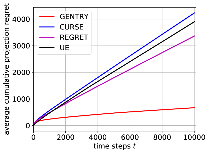
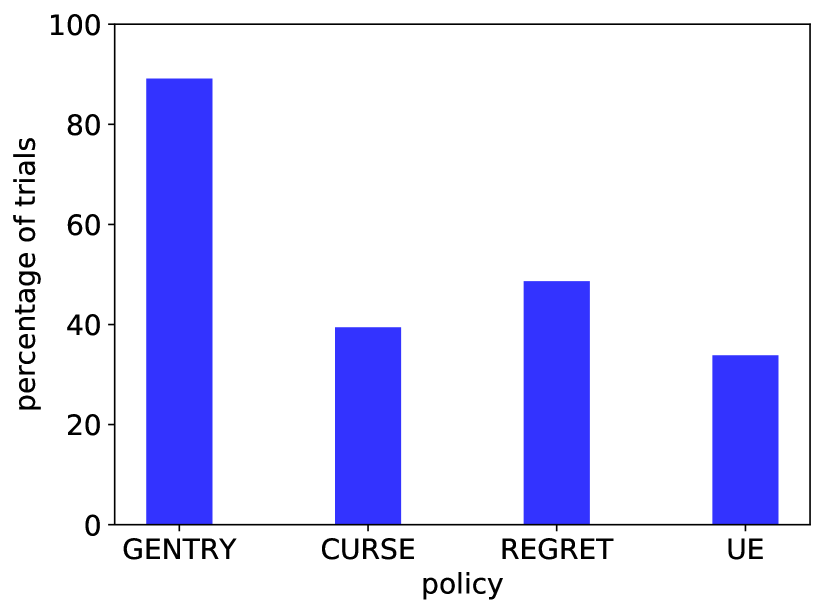
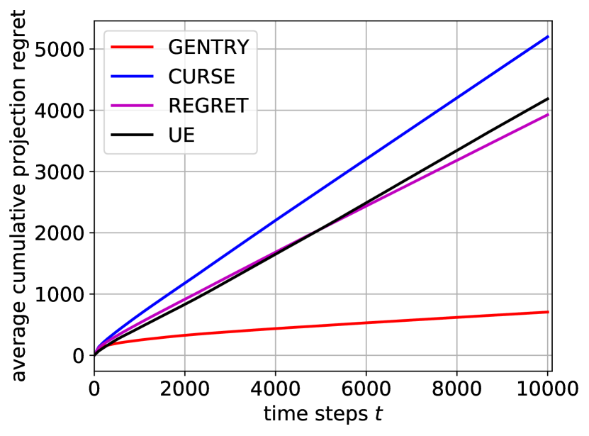
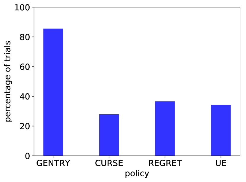
In this section, we verify the efficiency of our strategy by performing simulations on synthetic data and a wine quality dataset[35]. We compare against the following strategies:

  1. 1)

    the Uncertainty Ellipsoid (UE) policy [15], which chooses

    argmax𝐱𝔻r¯t1(𝐱)+αlogtmin{dlogt,|𝔻|}𝐱𝐕t11subscriptargmax𝐱𝔻subscript¯𝑟𝑡1𝐱𝛼𝑡𝑑𝑡𝔻subscriptnorm𝐱superscriptsubscript𝐕𝑡11\operatorname*{arg\,max}_{\mathbf{x}\in\mathbb{D}}\bar{r}_{t-1}(\mathbf{x})+\alpha\sqrt{\log t\min\{d\log t,|\mathbb{D}|\}}\|\mathbf{x}\|_{\mathbf{V}_{t-1}^{-1}}

    at each time step t𝑡t;

  2. 2)

    the CorrUpted GReedy StratEgy (CURSE) by replacing argmax𝐱𝔻r¯t1(𝐱)subscriptargmax𝐱𝔻subscript¯𝑟𝑡1𝐱\operatorname*{arg\,max}_{\mathbf{x}\in\mathbb{D}}\bar{r}_{t-1}(\mathbf{x}) with argmax𝐱𝔻𝐱,𝜽^t1subscriptargmax𝐱𝔻𝐱subscript^𝜽𝑡1\operatorname*{arg\,max}_{\mathbf{x}\in\mathbb{D}}{\left\langle{\mathbf{x}},\,{\hat{\bm{\theta}}_{t-1}}\right\rangle} in GENTRY, i.e., the corruption in the observed return is not accounted for; and

  3. 3)

    the caRelEss GReEdy sTrategy (REGRET) where the Xisubscript𝑋𝑖X_{i} in GENTRY are all replaced by P𝕌(Xi)subscript𝑃𝕌subscript𝑋𝑖P_{\mathbb{U}}(X_{i}). To avoid any doubts, the full REGRET is shown in Algorithm 2.

Algorithm 2 REGRET
0:  Set ϵtsubscriptitalic-ϵ𝑡\epsilon_{t} to ϵtfsuperscriptsubscriptitalic-ϵ𝑡𝑓\epsilon_{t}^{f} or ϵtisuperscriptsubscriptitalic-ϵ𝑡𝑖\epsilon_{t}^{i} according to the number of arms; set hyper parameter α>0𝛼0\alpha>0 and λ>0𝜆0\lambda>0.
1:  loop
2:     Update ϵtsubscriptitalic-ϵ𝑡\epsilon_{t}.
3:     With probability 1ϵt1subscriptitalic-ϵ𝑡1-\epsilon_{t}, choose
argmax𝐱𝔻P𝕌(𝐱),P𝕌(𝜽~t1),subscriptargmax𝐱𝔻subscript𝑃𝕌𝐱subscript𝑃𝕌subscript~𝜽𝑡1\displaystyle\operatorname*{arg\,max}_{\mathbf{x}\in\mathbb{D}}{\left\langle{P_{\mathbb{U}}(\mathbf{x})},\,{P_{\mathbb{U}}(\tilde{\bm{\theta}}_{t-1})}\right\rangle},
where
𝜽~t=(i=1tP𝕌(Xi)P𝕌(Xi)+λ𝐈)1i=1triP𝕌(Xi),subscript~𝜽𝑡superscriptsuperscriptsubscript𝑖1𝑡subscript𝑃𝕌subscript𝑋𝑖subscript𝑃𝕌superscriptsubscript𝑋𝑖𝜆𝐈1superscriptsubscript𝑖1𝑡subscript𝑟𝑖subscript𝑃𝕌subscript𝑋𝑖\displaystyle\tilde{\bm{\theta}}_{t}=\left(\sum_{i=1}^{t}P_{\mathbb{U}}(X_{i})P_{\mathbb{U}}(X_{i})^{\intercal}+\lambda\mathbf{I}\right)^{-1}\sum_{i=1}^{t}r_{i}P_{\mathbb{U}}(X_{i}),
and with probability ϵtsubscriptitalic-ϵ𝑡\epsilon_{t} choose a random arm from 𝔻ksubscript𝔻𝑘\mathbb{D}_{k}.
4:     Update P𝕌(𝐱),P𝕌(𝜽~t1)subscript𝑃𝕌𝐱subscript𝑃𝕌subscript~𝜽𝑡1{\left\langle{P_{\mathbb{U}}(\mathbf{x})},\,{P_{\mathbb{U}}(\tilde{\bm{\theta}}_{t-1})}\right\rangle}. Set t=t+1𝑡𝑡1t=t+1.
5:  end loop

In each simulation, we perform 200020002000 trials, each with 104superscript10410^{4} time steps. To compare the projection regret performance of different strategies, we compute the average empirical cumulative projection regret over all the trials. For convenience, this average is referred to as the average cumulative projection regret.

IV-A Experiments on Synthetic Data

In this section, we compare the performance of different strategies using synthetic data. We use three settings in the simulations:

  1. (a)

    For the finite-arm case, in each trial, we generate the decision set 𝔻d𝔻superscript𝑑\mathbb{D}\subseteq\mathbb{R}^{d} containing K𝐾K arms, in which each arm is associated with a d𝑑d-dimension feature vector. Each dimension of the feature vector is drawn i.i.d. from the uniform distribution 𝒰(1,1)𝒰11\mathcal{U}(-1,1). Each dimension of the ground-truth parameter 𝜽𝜽\bm{\theta} is also drawn from 𝒰(1,1)𝒰11\mathcal{U}(-1,1). We next generate the orthogonal projection matrix P𝕌=𝐀(𝐀𝐀)1𝐀subscript𝑃𝕌𝐀superscriptsuperscript𝐀𝐀1superscript𝐀P_{\mathbb{U}}=\mathbf{A}(\mathbf{A}^{\intercal}\mathbf{A})^{-1}\mathbf{A}^{\intercal}, where 𝐀𝐀\mathbf{A} is a d×u𝑑𝑢d\times u (u<d𝑢𝑑u<d) matrix whose elements are generated randomly from 𝒰(1,1)𝒰11\mathcal{U}(-1,1). The noise ηtsubscript𝜂𝑡\eta_{t} at each time step is drawn i.i.d. from the Gaussian distribution 𝒩(0,ϑ2)𝒩0superscriptitalic-ϑ2\mathcal{N}(0,\vartheta^{2}) with variance ϑ2superscriptitalic-ϑ2\vartheta^{2}. The decision set 𝔻𝔻\mathbb{D}, parameter 𝜽𝜽\bm{\theta} and projection matrix P𝕌subscript𝑃𝕌P_{\mathbb{U}} are fixed in each trial.

  2. (b)

    We use the same setting as in setting a except that the projection matrix P𝕌subscript𝑃𝕌P_{\mathbb{U}} in this setting is a diagonal matrix whose (i,i)𝑖𝑖(i,i) entry is 111 for i=1,,u𝑖1𝑢i=1,\cdots,u and 00 otherwise. This means that the last du𝑑𝑢d-u dimensions of 𝜽𝜽\bm{\theta} are the protected features.

  3. (c)

    For the infinite-arm case, in each trial, the decision set 𝔻𝔻\mathbb{D} is limited to a convex set for ease of computation. Specifically, we use the convex set 𝔻𝔻\mathbb{D}:

    𝔻={𝐱:i=1d𝐱(i)log𝐱(i)5 and 𝐱(i)0i},𝔻conditional-set𝐱superscriptsubscript𝑖1𝑑𝐱𝑖𝐱𝑖5 and 𝐱𝑖0for-all𝑖\displaystyle\mathbb{D}=\left\{\mathbf{x}:\sum_{i=1}^{d}\mathbf{x}(i)\log\mathbf{x}(i)\leq 5\text{ and }\mathbf{x}(i)\geq 0\ \forall\ i\right\}, (45)

    where 𝐱(i)𝐱𝑖\mathbf{x}(i) is the i𝑖i-th entry of 𝐱𝐱\mathbf{x}, 0log0:=0assign0000\log 0:=0, and 𝜽𝜽\bm{\theta}, P𝕌subscript𝑃𝕌P_{\mathbb{U}} and ηtsubscript𝜂𝑡\eta_{t} are generated the same way as in setting a.

In the following, GENTRY, CURSE, and REGRET use the setting ϵ=ϵtfitalic-ϵsuperscriptsubscriptitalic-ϵ𝑡𝑓\epsilon=\epsilon_{t}^{f} described in Section III when in setting a and b for the finite-arm case. Accordingly, ϵ=ϵtiitalic-ϵsuperscriptsubscriptitalic-ϵ𝑡𝑖\epsilon=\epsilon_{t}^{i} is used when in setting c for the infinite-arm case. In all simulations, the parameter λ𝜆\lambda is set to 111.

IV-A1 Varying α𝛼\alpha

Refer to caption
(a) Using setting a with d=10𝑑10d=10, K=45𝐾45K=45, and u=5𝑢5u=5
Refer to caption
(b) Using setting c with d=4𝑑4d=4, and u=2𝑢2u=2
Fig. 1: Regret comparison between different strategies with ϑ=0.5italic-ϑ0.5\vartheta=0.5 and varying α𝛼\alpha.

All the strategies depend on the hyperparameter α𝛼\alpha, with a larger α𝛼\alpha corresponding to more exploration on average. We do simulations using setting a with d=10𝑑10d=10, K=45𝐾45K=45, ϑ=0.5italic-ϑ0.5\vartheta=0.5, u=5𝑢5u=5, and setting c with d=4𝑑4d=4, ϑ=0.5italic-ϑ0.5\vartheta=0.5, u=2𝑢2u=2. Figs. 1(a) and 1(b) show how the average cumulative projective regret at time step 104superscript10410^{4} changes with different α𝛼\alpha in each strategy. We observe the following:

  • We note that a moderate α𝛼\alpha is optimal for each strategy. When α𝛼\alpha is too large, the strategy explores too frequently, leading to a large projection regret as expected. On the other hand, a small α𝛼\alpha results in little exploration, and good arms cannot be found efficiently.

  • In Fig. 1(a), GENTRY with α=1𝛼1\alpha=1 outperforms all the other benchmark strategies. This is because the other strategies do not achieve an asymptotically unbiased estimation of the projection reward. Fig. 1(b) shows similar results.

In the following simulations, for a fair comparison, we tune the parameter α𝛼\alpha for each strategy to achieve the best average asymptotic cumulative projection regret for that strategy. Specifically, we set α=1𝛼1\alpha=1 for all the strategies except UE, which is given a α=0.1𝛼0.1\alpha=0.1 when using setting a and b. When using setting c, we set α=0.01𝛼0.01\alpha=0.01 for all the strategies except REGRET, which is given a α=0.1𝛼0.1\alpha=0.1.

IV-A2 Results and Analysis

Refer to caption
(a) Average cumulative projection regret
Refer to caption
(b) Percentage of trials where the best decision is found
Fig. 2: Performance comparison between different strategies using setting a with d=10𝑑10d=10, K=45𝐾45K=45, ϑ=0.5italic-ϑ0.5\vartheta=0.5 and u=5𝑢5u=5.
Refer to caption
(a) Average cumulative projection regret
Refer to caption
(b) Percentage of trials where the best decision is found
Fig. 3: Performance comparison between different strategies using setting b with d=10𝑑10d=10, K=45𝐾45K=45, ϑ=0.5italic-ϑ0.5\vartheta=0.5 and u=5𝑢5u=5.

In the simulations for the finite-arm case using settings a and b, we set d=10𝑑10d=10, K=45𝐾45K=45, ϑ=0.5italic-ϑ0.5\vartheta=0.5 and u=5𝑢5u=5. The simulation results are shown in Figs. 2 and 3. We observe the following:

  • The average cumulative projection regrets of different strategies are shown in Figs. 2(a) and 3(a). We see that GENTRY has obvious sublinear cumulative projection regret performance. The other benchmark strategies all suffer from a linearly increasing cumulative projection regret. This verifies that if our objective is to maximize the cumulative projection reward instead of the cumulative return (including the corruption), GENTRY is more appropriate.

  • Figs. 2(b) and 3(b) show the percentage of trials in which the optimal arm is chosen for more than 90%percent9090\% of the time in the last 200200200 time steps. We see that GENTRY finds the optimal arm in most trials, and outperforms the other strategies by a significant margin.

In the simulations for the infinite-arm case using setting c, we set d=4𝑑4d=4, ϑ=0.5italic-ϑ0.5\vartheta=0.5 and u=2𝑢2u=2. From Fig. 4, we also observe that GENTRY has obvious sublinear cumulative projection regret performance. The other benchmark strategies have linearly increasing cumulative projection regret. This verifies the efficiency of GENTRY for the infinite-arm case.
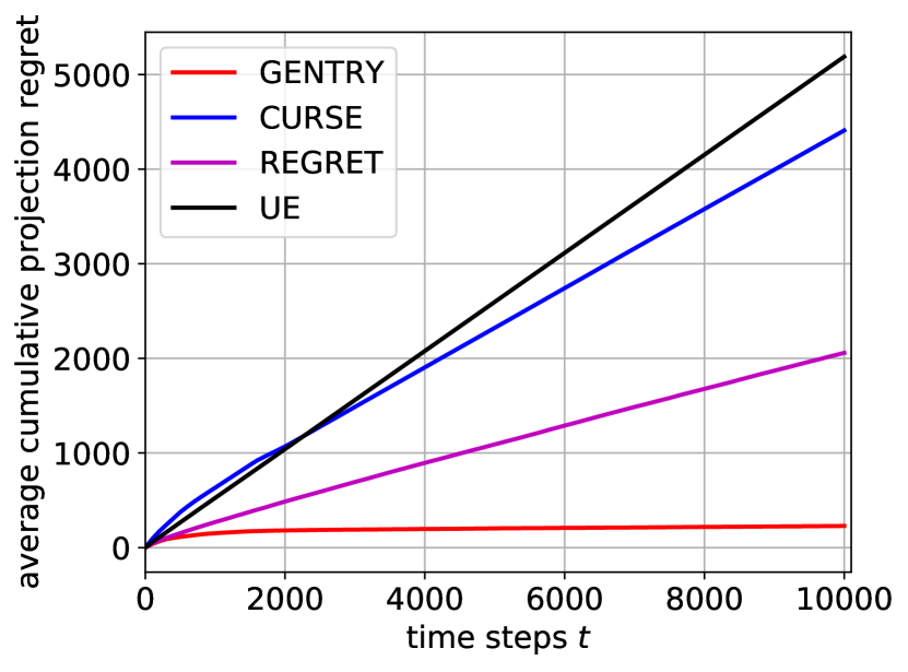
Refer to caption
Fig. 4: Average cumulative projection regret using setting c with d=4𝑑4d=4, u=2𝑢2u=2 and ϑ=0.5italic-ϑ0.5\vartheta=0.5.

IV-B Experiments on Wine Quality Dataset

We next compare the performance of different strategies using the wine quality dataset, which contains 111111-dimension description vectors of 489848984898 white wines and their ratings (scores between 00 and 101010). In each trial, we randomly select 200200200 wines with ratings 444, 555, 666, 777 and 888, as the decision set 𝔻𝔻\mathbb{D}, since among all the wines there are only 555 wines with ratings larger than 888 and 202020 wines with ratings less than 444. Each dimension of the wine description vector is a physicochemical characteristic like volatile acidity, chlorides, or density. Due to privacy and logistic issues[35], only the physicochemical characteristics and ratings are available (e.g., there is no data about grape types, wine brand, wine selling price, etc.). We add one additional feature drawn i.i.d. from 𝒰(0,1)𝒰01\mathcal{U}(0,1) as the protected feature. The corresponding rating of each wine is then corrupted by subtracting 444 times this protected feature value from the original rating. In this experiment, we take the original rating as the projection reward. Finally, we add a constant 111 as the constant feature to each description vector. If we put the protected feature as the final dimension of each wine, then d=13𝑑13d=13, and the projection matrix P𝕌subscript𝑃𝕌P_{\mathbb{U}} is defined as a diagonal matrix whose (i,i)𝑖𝑖(i,i) entry is 1 for i=1,,12𝑖112i=1,\cdots,12, and 00 for i=13𝑖13i=13. As there are finitel many arms, we use ϵ=ϵtfitalic-ϵsuperscriptsubscriptitalic-ϵ𝑡𝑓\epsilon=\epsilon_{t}^{f} in this experiment. The results are shown in Fig. 5, from which we observe that GENTRY outperforms all the other strategies.
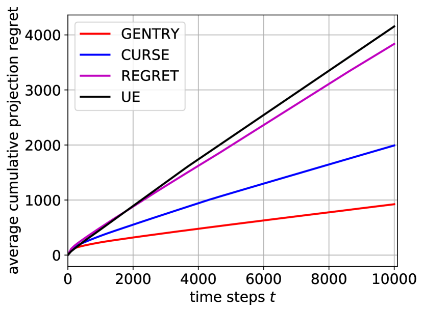
Refer to caption
Fig. 5: Average cumulative projection regret using the wine quality dataset.

V Conclusion

We have formulated the orthogonal projection problem in the linear stochastic bandit model, where the objective is to maximize the cumulative projection reward over a subspace of decision attributes based on observed returns that consist of the projection reward with corruption. Our proposed GENTRY achieves sublinear projection regret for the finite- and infinite-arm cases. Experiments verify the efficiency of our strategy. Our formulation and strategy are useful in avoiding discrimination in recommendation systems and in mixed drug treatment trials.

In this paper, we have assumed that the target subspace is known beforehand when decomposing the reward. However, in practice, we may not know what is a suitable projection subspace a priori. It is of interest in future research to develop methods to learn this subspace in conjunction with the best arm using possibly additional side-information.

References

  • [1] H. Robbins, “Some aspects of the sequential design of experiments,” Bull. Amer. Math. Soc., vol. 58, no. 5, pp. 527–535, Jul. 1952.
  • [2] P. Auer, N. Cesa-Bianchi, and P. Fischer, “Finite–time analysis of the multiarmed bandit problem,” Mach. Learn., vol. 47, no. 2, pp. 235–256, May 2002.
  • [3] T. L. Lai and H. Robbins, “Asymptotically efficient adaptive allocation rules,” Advances Appl. Math., vol. 6, no. 1, pp. 4–22, Mar. 1985.
  • [4] J.-Y. Audibert, R. Munos, and C. Szepesvári, “Exploration–exploitation tradeoff using variance estimates in multi-armed bandits,” Theoretical Comput. Sci., vol. 410, no. 19, pp. 1876–1902, Oct. 2009.
  • [5] R. Agrawal, “Sample mean based index policies by O(log n) regret for the multi-armed bandit problem,” Advances Appl. Probability, vol. 27, no. 4, pp. 1054–1078, Dec. 1995.
  • [6] A. N. Burnetas and M. N. Katehakis, “Optimal adaptive policies for sequential allocation problems,” Advances Appl. Math., vol. 17, no. 2, pp. 122–142, Jun. 1996.
  • [7] Q. Kang and W. P. Tay, “Task recommendation in crowdsourcing based on learning preferences and reliabilities,” arXiv preprint arXiv:1807.10444, 2018.
  • [8] Y. Liu and M. Liu, “An online learning approach to improving the quality of crowd-sourcing,” IEEE/ACM Trans. Netw., vol. 25, no. 4, pp. 2166–2179, Aug 2017.
  • [9] S. Klos née Müller, C. Tekin, M. van der Schaar, and A. Klein, “Context-aware hierarchical online learning for performance maximization in mobile crowdsourcing,” IEEE/ACM Trans. Netw., vol. 26, no. 3, pp. 1334–1347, June 2018.
  • [10] Q. Kang and W. P. Tay, “Sequential multi-class labeling in crowdsourcing,” IEEE Trans. Knowl. Data Eng., vol. 31, no. 11, pp. 2190 – 2199, Nov. 2019.
  • [11] S. Pandey, D. Chakrabarti, and D. Agarwal, “Multi-armed bandit problems with dependent arms,” in Proc. Int. Conf. Mach. Learn., Oregon, USA, Jun. 2007, pp. 721–728.
  • [12] E. L. Presman, Sonin, I. N, and Sonin, Sequential Control with Incomplete Information.   London, UK: Academic Press, 1990.
  • [13] A. Goldenshluger, A. Zeevi et al., “Woodroofe’s one-armed bandit problem revisited,” Ann. Appl. Probability, vol. 19, no. 4, pp. 1603–1633, Nov. 2009.
  • [14] Y. Abbasi-Yadkori, D. Pál, and C. Szepesvári, “Improved algorithms for linear stochastic bandits,” in Proc. Advances Neural Inf. Process. Syst., Granada, Spain, Dec. 2011, pp. 2312–2320.
  • [15] P. Rusmevichientong and J. N. Tsitsiklis, “Linearly parameterized bandits,” Math. Oper. Res., vol. 35, no. 2, pp. 395–411, May 2010.
  • [16] Y. Gai, B. Krishnamachari, and R. Jain, “Combinatorial network optimization with unknown variables: Multi-armed bandits with linear rewards and individual observations,” IEEE/ACM Trans. Netw., vol. 20, no. 5, pp. 1466–1478, Oct 2012.
  • [17] S. Agrawal and N. Goyal, “Thompson sampling for contextual bandits with linear payoffs,” in Proc. Int. Conf. Mach. Learn., Georgia, USA, Jun. 2013, pp. 127–135.
  • [18] L. Li, W. Chu, J. Langford, and R. E. Schapire, “A contextual-bandit approach to personalized news article recommendation,” in Proc. Int. Conf. World Wide Web, New York, USA, Apr. 2010, pp. 661–670.
  • [19] N. Abe, A. W. Biermann, and P. M. Long, “Reinforcement learning with immediate rewards and linear hypotheses,” Algorithmica, vol. 37, no. 4, pp. 263–293, Dec. 2003.
  • [20] Y. Yue and C. Guestrin, “Linear submodular bandits and their application to diversified retrieval,” in Proc. Advances Neural Inf. Process. Syst., Granada, Spain, Dec. 2011, pp. 2483–2491.
  • [21] S. S. Villar, J. Bowden, and J. Wason, “Multi-armed bandit models for the optimal design of clinical trials: Benefits and challenges,” Statist. Sci., vol. 30, no. 2, p. 199, May 2015.
  • [22] V. Dani, T. P. Hayes, and S. M. Kakade, “Stochastic linear optimization under bandit feedback,” in Proc. Annu. Conf. Learn. Theory, Helsinki, Finland, Jul. 2008, pp. 355–366.
  • [23] V. Kuleshov and D. Precup, “Algorithms for multi-armed bandit problems,” arXiv preprint arXiv:1402.6028, 2014.
  • [24] Why netflix features black actors in promos to black users. Accessed: Jun. 25, 2019. [Online]. Available: https://www.wired.com/story/why-netflix-features-black-actors-promos-to-black-users
  • [25] R. D. Toto, “Treatment of hypertension in chronic kidney disease,” Seminars Nephrology, vol. 25, no. 6, pp. 435–439, Nov. 2005.
  • [26] P. Auer, “Using confidence bounds for exploitation-exploration trade-offs,” J. Mach. Learn. Res., vol. 3, no. 11, pp. 397–422, Nov. 2002.
  • [27] H. Wang, Q. Wu, and H. Wang, “Learning hidden features for contextual bandits,” in Proc. Int. Conf. Inform. Knowl. Manag., Indianapolis, USA, Oct. 2016, pp. 1633–1642.
  • [28] A. Uschmajew, “Local convergence of the alternating least squares algorithm for canonical tensor approximation,” J. Matrix Anal. Appl., vol. 33, no. 2, pp. 639–652, Jun. 2012.
  • [29] J. Friedman, T. Hastie, and R. Tibshirani, “Regularization paths for generalized linear models via coordinate descent,” J. Statist. Softw., vol. 33, no. 1, pp. 1–22, Aug. 2010.
  • [30] M. M. Drugan, A. Nowé, and B. Manderick, “Pareto upper confidence bounds algorithms: an empirical study,” in Proc. IEEE Symp. Adaptive Dynamic Programming Reinforcement Learn., Orlando, USA, Dec. 2014, pp. 1–8.
  • [31] M. M. Drugan and A. Nowe, “Designing multi-objective multi-armed bandits algorithms: A study,” in Proc. Int. Joint Conf. Neural Netw., Dallas, USA, Aug 2013, pp. 1–8.
  • [32] S. Q. Yahyaa, M. M. Drugan, and B. Manderick, “Annealing-pareto multi-objective multi-armed bandit algorithm,” in Proc. IEEE Symp. Adaptive Dynamic Programming Reinforcement Learn., Orlando, USA, Dec. 2014, pp. 1–8.
  • [33] ——, “The scalarized multi-objective multi-armed bandit problem: An empirical study of its exploration vs. exploitation tradeoff,” in Proc. Int. Joint Conf. Neural Netw., Beijing, China, Jul. 2014, pp. 2290–2297.
  • [34] E. Zitzler, L. Thiele, M. Laumanns, C. M. Fonseca, and V. Da Fonseca Grunert, “Performance assessment of multiobjective optimizers: An analysis and review,” IEEE Trans. Evol. Comput., vol. 139, no. 2, pp. 117–132, May 2002.
  • [35] P. Cortez, A. Cerdeira, F. Almeida, T. Matos, and J. Reis, “Modeling wine preferences by data mining from physicochemical properties,” Decision Support Syst., vol. 47, no. 4, pp. 547–553, May 2009.
  • [36] S. J. Leon, Linear Algebra with Applications.   Upper Saddle River, NJ: Pearson, 2010.
  • [37] T. Calders, A. Karim, F. Kamiran, W. Ali, and X. Zhang, “Controlling attribute effect in linear regression,” in Proc. Int. Conf. Data Mining, Dallas, USA, Dec. 2013, pp. 71–80.
  • [38] D. Pollard, Convergence of Stochastic Processes.   Berlin, DE: Springer, 1984.
  • [39] E. S. Polovinkin, “Strongly convex analysis,” Sbornik: Math., vol. 187, no. 2, p. 259, Feb. 1996.