Cache-Aided NOMA Mobile Edge Computing: A Reinforcement Learning Approach

Zhong Yang,  Yuanwei Liu, 
Yue Chen,  and Naofal Al-Dhahir
Part of this paper has been presented in IEEE International Communication Conference (ICC) 2019 [1]. Z. Yang, Y. Liu and Y. Chen are with the School of Electronic Engineering and Computer Science, Queen Mary University of London, London E1 4NS, UK. (email:{zhong.yang, yuanwei.liu, yue.chen}@qmul.ac.uk) N. Al-Dhahir is with the Department of Electrical and Computer Engineering, University of Texas at Dallas, Richardson, TX 75080. (email: aldhahir@utdallas.edu )
Abstract

A novel non-orthogonal multiple access (NOMA) based cache-aided mobile edge computing (MEC) framework is proposed. For the purpose of efficiently allocating communication and computation resources to users’ computation tasks requests, we propose a long-short-term memory (LSTM) network to predict the task popularity. Based on the predicted task popularity, a long-term reward maximization problem is formulated that involves a joint optimization of the task offloading decisions, computation resource allocation, and caching decisions. To tackle this challenging problem, a single-agent Q-learning (SAQ-learning) algorithm is invoked to learn a long-term resource allocation strategy. Furthermore, a Bayesian learning automata (BLA) based multi-agent Q-learning (MAQ-learning) algorithm is proposed for task offloading decisions. More specifically, a BLA based action select scheme is proposed for the agents in MAQ-learning to select the optimal action in every state. We prove that the BLA based action selection scheme is instantaneously self-correcting and the selected action is an optimal solution for each state. Extensive simulation results demonstrate that: 1) The prediction error of the proposed LSTMs based task popularity prediction decreases with increasing learning rate. 2) The proposed framework significantly outperforms the benchmarks like all local computing, all offloading computing and non-cache computing. 3) The proposed BLA based MAQ-learning achieves an improved performance compared to conventional reinforcement learning algorithms.

Index Terms:
Bayesian learning automata (BLA), multi-agent Q-learning (MAQ-learning), non-orthogonal multiple access (NOMA), mobile edge computing (MEC).

I Introduction

Mobile applications have been growing exponentially in wireless networks due to the explosive growth in smart wireless devices. The success of heterogeneous services and related applications, such as augmented reality (AR), virtual reality (VR), real-time online gaming and high-speed video streaming in wireless networks require unprecedented high access speed and low latency [2, 3]. However, the stringent performance and delay requirements of computationally-intensive and latency-sensitive applications are significantly restricted by limited battery capacity and computation resources of the mobile devices. To address these significant challenges, a new trend is emerging with the function of central networks being increasingly moved towards the network edges (see [4], and references therein). The key idea of mobile edge computing (MEC) is to promote abundant computing resources at the edge of networks by integrating MEC servers at wireless access points (APs). The computation tasks requested by mobile users can be offloaded to the APs, which liberates the mobile devices from heavy computation workloads and reduces their energy consumption. However, determining communication and computation resources at networks edge introduces significant challenges (see [3, 4], and references therein), such as task offloading decisions of mobile users, computing resource allocation of the APs to satisfy large numbers of computationally-intensive and latency-sensitive computing tasks..

For the transmission aspect: Non-orthogonal multiple access (NOMA) emerged recently as a key enabling technology for next generation wireless communication, thanks to its high bandwidth efficiency and ultra high connectivity [5, 6]. The key idea behind NOMA is to ensure that multiple users are served simultaneously within the same given time/frequency resource block (RB), utilizing superposition coding (SC) techniques at the transmitter and successive interference cancellation (SIC) at the receiver [7, 8]. Different from orthogonal multiple access (OMA) in MEC networks, NOMA based MEC enables the mobile users to offload the computation tasks to the MEC servers simultaneously, which significantly reduce the computation latency of the network. Therefore, adopting NOMA in MEC networks better utilizes the capacity of the communication channel for offloading computation tasks, and thus improves the computing performance for multiuser MEC networks.

For the computation aspect: Caching is another promising technique due to the strategy of trading spectrum resources with storage resources. The main idea behind caching is to place abundant cache resources at the network edge for storing reusable content. In MEC networks, the task computation results may be requested by other users in the near future [9, 10]. For instance, in real-time online gaming, a rendered game frame would be sent to a bunch of nearby users in the same game. Accordingly, caching reusable task computation results in the MEC server is capable of reducing the duplicated task offloading and computing, therefore, it releases the computation burden and latency of the MEC networks [11, 12].

I-A Related Works

1) Studies on NOMA MEC networks: In contrast to the conventional OMA based MEC, the NOMA based MEC enables simultaneous task offloading, thus reducing energy consumption and avoiding delay. This motivated numerous researchers to dedicate substantial research contributions to NOMA MEC networks [13, 14, 15, 16, 17, 18]. Various asymptotic studies are carried out in [13], revealing that the impact of channel conditions and transmit powers on NOMA MEC are different from conventional NOMA scenarios. For one AP scenario, the authors in [14] jointly optimized the communication and computation resource allocation as well as the BS’s successive interference cancelation (SIC) decoding order, to minimize the total energy consumption of the users. In [15], the energy consumption of the users is minimized via optimizing the user clustering, computing and communication resource allocation, and transmit powers. Different from [14, 15], which only consider the uplink task transmission, the authors exploited NOMA for both task uploading and result downloading in [16]. Different from [14, 15, 16], which minimize the energy consumption, the authors in [17] minimized the offloading delay in a two-user NOMA MEC network. For the multiple APs scenario, a joint radio and computational resource allocation problem is investigated in [18], aiming at minimizing the energy consumption of all users under the task execution latency in heterogeneous networks. The above works on NOMA MEC analyze the static NOMA MEC networks using stochastic geometry approaches. However, for dynamic NOMA MEC networks, the uncertainty and unavailability of prior information makes conventional approaches difficult or even impossible.

2) Studies on NOMA Caching networks: The flexibility of NOMA makes it easy to integrate with other emerging wireless technologies like caching, to enable spectral and energy efficient transmission [19]. In [20], the NOMA strategy is utilized in caching networks, for pushing more contents to the server or simultaneously pushing the contents to the server and users. In [21], the cache-aided NOMA scheme is proposed to improve the coverage performance of NOMA communications. The authors in [8, 22] proposed a cache-aided NOMA scheme, to exploit cached data for interference cancellation in NOMA transmission. In [23], cache-aided NOMA is proposed to reduce the outage probability when a user possesses a cache of information requested by a user with a stronger channel. Different from [19, 20, 21, 8, 22, 23], which adopt superposition coding (SC) at the transmitters, the authors in [24] utilize index coding (IC) in cache-aided NOMA networks for reducing the transmission power.

3) Studies on Caching MEC networks: Wireless caching is typically employed in MEC networks, for supporting multimedia contents in networks edge to reduce the computing overhead and latency [25]. The motivation for integrating caching and computing for next generation wireless networks is to facilitate massive content delivery and satiate the requirements of network conditions and mobile devices. Both a cache-assisted computing mechanism and a computing-assisted caching mechanism are proposed in [26].

I-B Motivation

While the aforementioned research contributions have laid a solid foundation for caching, NOMA and MEC networks, the investigations on the applications of integrating caching and NOMA in MEC networks are still in their infancy. It is worth pointing out that, in a multi-users MEC network, where there are several users requesting services from one AP, the major challenge is computing model selection (i.e., local computing or MEC computing) and computation resource allocation. Due to the combinatorial nature of computing mode selection, the task offloading and resource allocation problem is generally formulated as a mixed integer programming (MIP) problem. To tackle this MIP problem, branch-and-bound algorithms [27] and dynamic programming [28] are adopted for the globally optimal solution. Though the conventional approaches make solid contributions to static optimization of task offloading and resource allocation, the mobile users nowadays request dynamic task computing, which is non-trivial for conventional approaches. Furthermore, designing the apriori resource allocation scheme in a long-term manner is nontrivial or even impossible for conventional approaches.

With the development of reinforcement learning (RL) and the high computing speed of new workstations, the investigations on the applications of RL algorithms in wireless networks are growing rapidly [29]. RL is a promising approach to find an efficient long-term resource allocation solution in an intelligent manner. In cache-aided NOMA MEC networks, the task popularity prediction is the key foundation to efficiently serve mobile users’ dynamic requests.

1) For the prediction problem: Long short-term memory (LSTM) networks are utilized in [30] to predict the traffic patterns at different timescales. In [31], LSTMs are adopted to predict reference information in statistical script. A new spatiotemporal LSTM model is utilized in [32] to generate future images by learning from the historical frames for spatiotemporal sequences.

2) For the resource allocation problem: A model-free deep reinforcement learning (DRL) approach is proposed in [33] to efficiently allocate resources upon users’ requests and price the resource usage. In [34], the server selection problem is formulated as a budget-constrained multi-armed bandit (MAB) problem, where each agent is given a reward and cost. A Bayesian reinforcement learning (BRL) algorithm is proposed in [35] for a distributed resource sharing problem in a heterogeneous network, which shows a superior performance compared with other resource allocation schemes. It is worth pointing out that the characteristics of cache-aided NOMA MEC networks make it challenging to apply the RL algorithms, because the number of states increase exponentially with the number of users and tasks, which we have demonstrated in our previous work [36]. In this paper, our goal is to answer the following key questions:

  1. \bullet

    𝐐𝐮𝐞𝐬𝐭𝐢𝐨𝐧𝟏::𝐐𝐮𝐞𝐬𝐭𝐢𝐨𝐧1absent\bf Question~{}1: Do cache-aided NOMA MEC networks significantly outperform non-cached NOMA MEC networks?

  2. \bullet

    𝐐𝐮𝐞𝐬𝐭𝐢𝐨𝐧𝟐::𝐐𝐮𝐞𝐬𝐭𝐢𝐨𝐧2absent\bf Question~{}2: Do NOMA enhanced MEC networks bring energy reduction compared with conventional OMA based networks?

  3. \bullet

    𝐐𝐮𝐞𝐬𝐭𝐢𝐨𝐧𝟑::𝐐𝐮𝐞𝐬𝐭𝐢𝐨𝐧3absent\bf Question~{}3: Do BLA based MAQ-learning algorithm achieve better performance than conventional RL algorithms?

I-C Contributions and Organization

Being motivated to answer the above questions, in this paper, we design a cache-aided NOMA MEC framework, in which cache and computation resources are integrated for computationally-intensive and latency-sensitive tasks. In our proposed framework, we formulate the considered problem as a long-term reward maximization problem that entails joint optimization of task offloading decisions, computation resource allocation and caching decisions. Instead of solving a sophisticated joint optimization problem, the proposed algorithms are capable of learning from the past experience and automatically improve the allocation policy. In this paper, we propose a Bayesian learning automata (BLA) based multi-agent Q-learning (MAQ-learning) algorithm to improve the performance. Furthermore, we utilize the LSTM to predict the task popularity, while in [1], the task popularity is assumed to follow a Zipf distribution. Our main contributions are summarized as follows

  1. \bullet

    We propose a cache-aided NOMA MEC framework to reduce energy consumption. We establish the correlation between task popularity and cache-aided NOMA MEC, by modeling the cache-aided NOMA MEC with task popularity. We formulate a long-term energy minimization problem that jointly optimizes task offloading, computation and cache resource allocation.

  2. \bullet

    We propose a LSTM algorithm for task popularity prediction. The task popularity prediction is formulated as a time series prediction problem. We derive the weight value update expressions of LSTM based on a real-time recurrent learning (RTRL) algorithm, due to its low complexity in our proposed task popularity prediction problem.

  3. \bullet

    We formulate the total energy consumption as the reward function in the proposed RL algorithms. We prove that the Bayesian learning automata (BLA) based action selection scheme is instantaneously self-correcting and the selected action is an optimal solution for each state.

  4. \bullet

    We demonstrate that the proposed cache-aided NOMA MEC framework outperforms the other benchmark schemes such as non-cache MEC networks. The proposed algorithms achieve a performance improvement compared to MAQ-learning algorithms.

The rest of this paper is organized as follows. In Section II, the system model for the proposed cache-aided NOMA MEC framework is presented. In Section III, the LSTMs based task popularity prediction is investigated. The proposed algorithms for cache-aided NOMA MEC is given in Section IV. Simulation results are presented in Section V, before we conclude this work in Section VI. Table I provides a summary of the notations used in this paper.

TABLE I: LIST OF NOTATIONS
Notation Description Notation Description
𝒩usubscript𝒩𝑢{\mathcal{N}_{u}} the mobile users Ntsubscript𝑁𝑡N_{t} the computation tasks
B𝐵B the bandwidth between the AP and users σ2superscript𝜎2{{\sigma^{2}}} the power of additive noise
CMECsubscript𝐶MEC{C_{{\rm{MEC}}}} the computing capacities of the AP CCachesubscript𝐶Cache{C_{{\rm{Cache}}}} the caching capacities of the AP
πjsubscript𝜋𝑗{{\pi_{j}}} the size of the input of task j𝑗j (in bits) 𝐓𝐢,𝐣𝐨𝐟𝐟𝐥𝐨𝐚𝐝(𝐭)superscriptsubscript𝐓𝐢𝐣𝐨𝐟𝐟𝐥𝐨𝐚𝐝𝐭{\bf{T}}_{{\bf{i}},{\bf{j}}}^{{\bf{offload}}}\left({\bf{t}}\right) the offloading time for task j𝑗j
ωjsubscript𝜔𝑗{{\omega_{j}}} the computing capability required for this task 𝐄𝐢,𝐣𝐨𝐟𝐟𝐥𝐨𝐚𝐝(𝐭)superscriptsubscript𝐄𝐢𝐣𝐨𝐟𝐟𝐥𝐨𝐚𝐝𝐭{\bf{E}}_{{\bf{i}},{\bf{j}}}^{{\bf{offload}}}\left({\bf{t}}\right) the transmit energy consumption of offloading
κjsubscript𝜅𝑗{{\kappa_{j}}} Caching capacity 𝐓𝐢,𝐣𝐥𝐨𝐜superscriptsubscript𝐓𝐢𝐣𝐥𝐨𝐜{\bf{T}}_{{\bf{i}},{\bf{j}}}^{{\bf{loc}}} local computing time for task j𝑗j
σ2superscript𝜎2{\sigma^{2}} the computation result of task j𝑗j (in bits) 𝐄𝐢,𝐣𝐥𝐨𝐜superscriptsubscript𝐄𝐢𝐣𝐥𝐨𝐜{\bf{E}}_{{\bf{i}},{\bf{j}}}^{{\bf{loc}}} energy consumption of local computing for task j𝑗j
𝐗(𝐭)𝐗𝐭{\bf{X}}\left({\bf{t}}\right) the task offloading decision 𝐓𝐢,𝐣𝐦𝐞𝐜(𝐭)superscriptsubscript𝐓𝐢𝐣𝐦𝐞𝐜𝐭{\bf T_{i,j}^{mec}\left(t\right)} MEC computing time for task j𝑗j
𝐘(𝐭)𝐘𝐭{\bf{Y}}\left({\bf{t}}\right) the computing resource allocation vector 𝐄𝐢,𝐣𝐦𝐞𝐜(𝐭)superscriptsubscript𝐄𝐢𝐣𝐦𝐞𝐜𝐭{\bf{E}}_{{\bf{i}},{\bf{j}}}^{{\bf{mec}}}\left({\bf{t}}\right) energy consumption of MEC computing for task j𝑗j
𝐙(t)𝐙𝑡{\bf{Z}}\left(t\right) the task computation results caching decision vector 𝐖𝐟subscript𝐖𝐟{\bf{{W_{f}}}} weights in the forgot gate of the LSTM
PrijsuperscriptsubscriptPr𝑖𝑗\Pr_{i}^{j} the probability that user i𝑖i requests for task j𝑗j 𝐛𝐟subscript𝐛𝐟{\bf{{b_{f}}}} bias in the forgot gate of the LSTM
hi(t)subscript𝑖𝑡{{h_{i}}\left(t\right)} the channel gain between user i𝑖i and the MEC server 𝐖𝐢subscript𝐖𝐢{\bf{W_{i}}} weights of the sigmoid gate in the input gate
𝐑𝐢(𝐭)subscript𝐑𝐢𝐭{\bf{R_{i}}\left(t\right)} the achievable transmit rate of user i𝑖i at time t𝑡t 𝐖𝐂subscript𝐖𝐂{\bf W_{C}} weights of the tanh gate in the input gate
ρi(t)subscript𝜌𝑖𝑡\rho_{i}\left(t\right) the transmit power of user i𝑖i 𝐛𝐢subscript𝐛𝐢{\bf{b_{i}}} bias of the sigmoid gate in the input gate
𝐛𝐂subscript𝐛𝐂{\bf b_{C}} bias of the tanh gate in the input gate μ𝐭subscript𝜇𝐭{\bf{\mu_{t}}} the learning rate

II System Model

II-A Network Model

Refer to caption
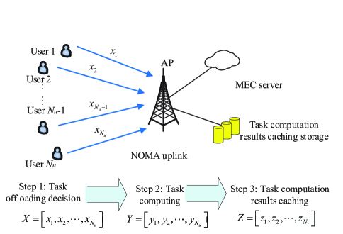
Figure 1: An illustration of multi-users cache-aided mobile edge computing networks.

As illustrated in Fig. 1, we consider a multi-user cache-aided MEC network with a single-antenna AP and N𝑁N single-antenna users, denoted as 𝒩u={1,,Nu}subscript𝒩𝑢1subscript𝑁𝑢{\mathcal{N}_{u}}=\left\{{1,\cdots,N_{u}}\right\}. The bandwidth between the AP and users is denoted by B𝐵B. The AP is associated with an MEC server using optical fiber, whose transmission delay can be ignored. The computing resources are partitioned into a resource pool to provide uniform resources granularity for the users. The AP has strong caching capability, which is capable of caching the computation results to serve other users who request the tasks in the future. The computing and caching capacities of the AP are denoted by CMECsubscript𝐶MEC{C_{{\rm{MEC}}}} and CCachesubscript𝐶Cache{C_{{\rm{Cache}}}}, respectively. Each user has a limited computation capacity and one intensive computation and sensitive latency computation task. Assume that there are Ntsubscript𝑁𝑡N_{t} computation tasks in the central network, denoted as 𝒩t={1,,Nt}subscript𝒩𝑡1subscript𝑁𝑡{\mathcal{N}_{t}}=\left\{{1,\cdots,N_{t}}\right\}. Each task j𝒩t𝑗subscript𝒩𝑡j\in{\cal N}_{t} is characterized by three parameters {πj,ωj,κj}subscript𝜋𝑗subscript𝜔𝑗subscript𝜅𝑗\left\{{{\pi_{j}},{\omega_{j}},{\kappa_{j}}}\right\}, which are defined as follows [11]:

  • πjsubscript𝜋𝑗{{\pi_{j}}} represents the size of the input of task j𝑗j (in bits);

  • ωjsubscript𝜔𝑗{{\omega_{j}}} represents the computing capability required for this task which is quantized by the number of CPU cycles;

  • κjsubscript𝜅𝑗{{\kappa_{j}}} represents the computation result of task j𝑗j (in bits).

The task offloading decision is denoted as 𝐗(𝐭)=[x1(t),x2(t),,xNu(t)]𝐗𝐭subscript𝑥1𝑡subscript𝑥2𝑡subscript𝑥subscript𝑁𝑢𝑡{\bf X\left(t\right)}=\left[{{x_{1}}\left(t\right),{x_{2}}\left(t\right),\cdots,{x_{{N_{u}}}}\left(t\right)}\right], where xi(t){0,1}subscript𝑥𝑖𝑡01{x_{i}}\left(t\right)\in\left\{{0,1}\right\}, xi(t)=0subscript𝑥𝑖𝑡0{x_{i}}\left(t\right)=0 means that the task of user i𝑖i is offloaded to the MEC server for computing, while xi(t)=1subscript𝑥𝑖𝑡1{x_{i}}\left(t\right)=1 means that the task is computed locally. The computing resource allocation vector is represented as 𝐘(𝐭)=[y1(t),y2(t),,yNu(t)]𝐘𝐭subscript𝑦1𝑡subscript𝑦2𝑡subscript𝑦subscript𝑁𝑢𝑡{\bf Y\left(t\right)}=\left[{{y_{1}}\left(t\right),{y_{2}}\left(t\right),\cdots,{y_{{N_{u}}}}\left(t\right)}\right], where yi(t)[0,1]subscript𝑦𝑖𝑡01{y_{i}}\left(t\right)\in\left[{0,1}\right] denotes that the computing resource proportion allocated to user i𝑖i from the AP. The task computation results caching decision vector is denoted as 𝐙(t)=[z1(t),z2(t),,zNt(t)]𝐙𝑡subscript𝑧1𝑡subscript𝑧2𝑡subscript𝑧subscript𝑁𝑡𝑡{\bf Z}\left(t\right)=\left[{{z_{1}}\left(t\right),{z_{2}}\left(t\right),\cdots,{z_{{N_{t}}}}\left(t\right)}\right], where zj(t){0,1}subscript𝑧𝑗𝑡01{z_{j}}\left(t\right)\in\left\{{0,1}\right\}, zj(t)=1subscript𝑧𝑗𝑡1{z_{j}}\left(t\right)=1 means that the computation result of task j𝑗j is cached, while zj(t)=0subscript𝑧𝑗𝑡0{z_{j}}\left(t\right)=0 means that the result is not cached. If the computation result is cached in the AP, the AP multicasts it to all users, thus reducing the offloading and computing workloads. The probability that user i𝑖i requests for task j𝑗j is denoted as Prij[0,1]superscriptsubscriptPr𝑖𝑗01\Pr_{i}^{j}\in\left[{0,1}\right] [9].

II-B Communication Model

In our NOMA transmission model, multiple users transmit their own uplink signals to the AP in the same RB. Therefore, the intercellular interference of the users in the same group is identical, the decoding order in one RB is determined only by the channel gains of users. Suppose that there are Nupsubscript𝑁𝑢𝑝N_{up} users who choose to upload their computation tasks, represented as 𝒩up={1,,Nup}subscript𝒩𝑢𝑝1subscript𝑁𝑢𝑝{{\cal N}_{up}}=\left\{{1,\cdots,{N_{up}}}\right\}, where Nup=i=1Nuxisubscript𝑁𝑢𝑝superscriptsubscript𝑖1subscript𝑁𝑢subscript𝑥𝑖{N_{up}}=\sum\nolimits_{i=1}^{N_{u}}{{x_{i}}}. Without loss of generality, assuming the users are ordered as follows:

|h1(t)|2|h2(t)|2|hNup(t)|2,superscriptsubscript1𝑡2superscriptsubscript2𝑡2superscriptsubscriptsubscript𝑁𝑢𝑝𝑡2{\left|{{h_{1}}\left(t\right)}\right|^{2}}\geq{\left|{{h_{2}}\left(t\right)}\right|^{2}}\geq\cdots\geq{\left|{{h_{{N_{up}}}}\left(t\right)}\right|^{2}}, (1)

where |hi(t)|2,i[1,Nup]superscriptsubscript𝑖𝑡2𝑖1subscript𝑁𝑢𝑝{\left|{{h_{i}}\left(t\right)}\right|^{2}},i\in\left[{1,{N_{up}}}\right] represents the channel gain between user i𝑖i and the MEC server.

In our NOMA scenario, the user with higher channel gain is decoded first, while the signal of lower channel gain user is considered as interference. Consider user i[1,Nup]𝑖1subscript𝑁𝑢𝑝i\in\left[{1,{N_{up}}}\right] who chooses to upload the computation task at time t𝑡t, then the achievable transmit rate 𝐑𝐢(𝐭)subscript𝐑𝐢𝐭{\bf{R_{i}}\left(t\right)} (in bits/s) is given by

𝐑𝐢(𝐭)=Blog2(1+ρi(t)|hi(t)|2l=i+1Nupρl(t)|hl(t)|2+σ2),subscript𝐑𝐢𝐭𝐵subscript21subscript𝜌𝑖𝑡superscriptsubscript𝑖𝑡2superscriptsubscript𝑙𝑖1subscript𝑁𝑢𝑝subscript𝜌𝑙𝑡superscriptsubscript𝑙𝑡2superscript𝜎2{{\bf{R}}_{\bf{i}}}\left({\bf{t}}\right)=B{\log_{2}}\left({1+\frac{{{\rho_{i}}\left(t\right){{\left|{{h_{i}}\left(t\right)}\right|}^{2}}}}{{\sum\limits_{l=i+1}^{{N_{up}}}{{\rho_{l}}\left(t\right){{\left|{{h_{l}}\left(t\right)}\right|}^{2}}}+{\sigma^{2}}}}}\right), (2)

where ρi(t)subscript𝜌𝑖𝑡\rho_{i}\left(t\right) denotes the transmit power of user i𝑖i, and σ2superscript𝜎2{{\sigma^{2}}} represents the power of additive noise. We assume that the users are randomly distributed in a square area. Accordingly, the offloading time for task j𝑗j with input size πjsubscript𝜋𝑗{\pi_{j}} at time t𝑡t is

𝐓𝐢,𝐣𝐨𝐟𝐟𝐥𝐨𝐚𝐝(𝐭)=πj𝐑𝐢(𝐭).superscriptsubscript𝐓𝐢𝐣𝐨𝐟𝐟𝐥𝐨𝐚𝐝𝐭subscript𝜋𝑗subscript𝐑𝐢𝐭{\bf T_{i,j}^{offload}\left(t\right)}=\frac{{{\pi_{j}}}}{\bf{{R_{i}}\left(t\right)}}. (3)

In addition, the transmit energy consumption of offloading at time t𝑡t is given by

𝐄𝐢,𝐣𝐨𝐟𝐟𝐥𝐨𝐚𝐝(𝐭)=ρiπj𝐑𝐢(𝐭).superscriptsubscript𝐄𝐢𝐣𝐨𝐟𝐟𝐥𝐨𝐚𝐝𝐭subscript𝜌𝑖subscript𝜋𝑗subscript𝐑𝐢𝐭{\bf{E}}_{{\bf{i}},{\bf{j}}}^{{\bf{offload}}}\left({\bf{t}}\right)={\rho_{i}}\frac{{{\pi_{j}}}}{{{{\bf{R}}_{\bf{i}}}\left({\bf{t}}\right)}}. (4)

II-C Computation Model

For the computation model, the task j𝑗j that user i𝑖i requests can be computed locally on the mobile device or offloaded to the MEC server for computing. Next, we consider the computation overhead in terms of processing time and energy consumption for both local computing and MEC computing.

II-C1 Local Computing

For user i𝑖i, the local computing capability (i.e. CPU cycles per second) is denoted by ωilocsuperscriptsubscript𝜔𝑖𝑙𝑜𝑐\omega_{i}^{loc}, and Pilocsuperscriptsubscript𝑃𝑖𝑙𝑜𝑐P_{i}^{loc} denotes the energy consumption per second for local computing at user i𝑖i. If task j𝑗j is computed locally, the computing time 𝐓𝐢,𝐣𝐥𝐨𝐜superscriptsubscript𝐓𝐢𝐣𝐥𝐨𝐜{\bf{T}}_{{\bf{i}},{\bf{j}}}^{{\bf{loc}}} for task j𝑗j with computational requirement ωjsubscript𝜔𝑗{{\omega_{j}}} is

𝐓𝐢,𝐣𝐥𝐨𝐜=ωjωiloc,superscriptsubscript𝐓𝐢𝐣𝐥𝐨𝐜subscript𝜔𝑗superscriptsubscript𝜔𝑖𝑙𝑜𝑐{\bf{T}}_{{\bf{i}},{\bf{j}}}^{{\bf{loc}}}=\frac{{{\omega_{j}}}}{{\omega_{i}^{loc}}}, (5)

Hereinafter, the energy consumption of local computing 𝐄𝐢,𝐣𝐥𝐨𝐜superscriptsubscript𝐄𝐢𝐣𝐥𝐨𝐜{\bf{E}}_{{\bf{i}},{\bf{j}}}^{{\bf{loc}}} of task j𝑗j is given by

𝐄𝐢,𝐣𝐥𝐨𝐜=Pilocωjωiloc,superscriptsubscript𝐄𝐢𝐣𝐥𝐨𝐜superscriptsubscript𝑃𝑖𝑙𝑜𝑐subscript𝜔𝑗superscriptsubscript𝜔𝑖𝑙𝑜𝑐{\bf{E}}_{{\bf{i}},{\bf{j}}}^{{\bf{loc}}}=P_{i}^{loc}\frac{{{\omega_{j}}}}{{\omega_{i}^{loc}}}, (6)

II-C2 MEC Computing

𝐄𝐢(t,xi(t),yi(t),zj(t))=(Prij(1zj(t))(xi(t)𝐄𝐢,𝐣𝐥𝐨𝐜+(1xi(t))𝐄𝐢,𝐣𝐨𝐟𝐟𝐥𝐨𝐚𝐝(𝐭)+(1yi(t))𝐄𝐢,𝐣𝐦𝐞𝐜(𝐭))).subscript𝐄𝐢𝑡subscript𝑥𝑖𝑡subscript𝑦𝑖𝑡subscript𝑧𝑗𝑡superscriptsubscriptPr𝑖𝑗1subscript𝑧𝑗𝑡subscript𝑥𝑖𝑡superscriptsubscript𝐄𝐢𝐣𝐥𝐨𝐜1subscript𝑥𝑖𝑡superscriptsubscript𝐄𝐢𝐣𝐨𝐟𝐟𝐥𝐨𝐚𝐝𝐭1subscript𝑦𝑖𝑡superscriptsubscript𝐄𝐢𝐣𝐦𝐞𝐜𝐭\displaystyle{{\bf{E}}_{\bf{i}}}\left({t,{x_{i}}\left(t\right),{y_{i}}\left(t\right),{z_{j}}\left(t\right)}\right)=\left({{\rm{Pr}}_{i}^{j}\left({1-{z_{j}}(t)}\right)\left({{x_{i}}(t){\bf{E}}_{{\bf{i}},{\bf{j}}}^{{\bf{loc}}}+\left({1-{x_{i}}(t)}\right){\bf{E}}_{{\bf{i}},{\bf{j}}}^{{\bf{offload}}}\left({\bf{t}}\right)+\left({1-{y_{i}}(t)}\right){\bf{E}}_{{\bf{i}},{\bf{j}}}^{{\bf{mec}}}\left({\bf{t}}\right)}\right)}\right). (7)

Let yi(t)[0,1]subscript𝑦𝑖𝑡01{y_{i}}\left(t\right)\in\left[{0,1}\right] denote the proportion of the computing resources that the AP allocated to user i𝑖i. The computing time 𝐓𝐢,𝐣𝐦𝐞𝐜(𝐭)superscriptsubscript𝐓𝐢𝐣𝐦𝐞𝐜𝐭{\bf T_{i,j}^{mec}\left(t\right)} for task j𝑗j at time t𝑡t is

𝐓𝐢,𝐣𝐦𝐞𝐜(𝐭)=ωjyi(t)CMEC.superscriptsubscript𝐓𝐢𝐣𝐦𝐞𝐜𝐭subscript𝜔𝑗subscript𝑦𝑖𝑡subscript𝐶𝑀𝐸𝐶{\bf{T}}_{{\bf{i}},{\bf{j}}}^{{\bf{mec}}}\left({\bf{t}}\right)=\frac{{{\omega_{j}}}}{{{y_{i}}\left(t\right){C_{MEC}}}}. (8)

The energy consumption per second for MEC server is denoted as Pmecsuperscript𝑃𝑚𝑒𝑐{P^{mec}}, thus the energy consumption 𝐄𝐢,𝐣𝐦𝐞𝐜(𝐭)superscriptsubscript𝐄𝐢𝐣𝐦𝐞𝐜𝐭{\bf E_{i,j}^{mec}\left(t\right)} of task j𝑗j computed in the AP is given by

𝐄𝐢,𝐣𝐦𝐞𝐜(𝐭)=Pmecωjyi(t)CMEC.superscriptsubscript𝐄𝐢𝐣𝐦𝐞𝐜𝐭superscript𝑃𝑚𝑒𝑐subscript𝜔𝑗subscript𝑦𝑖𝑡subscript𝐶𝑀𝐸𝐶{\bf E_{i,j}^{mec}\left(t\right)}={P^{mec}}\frac{{{\omega_{j}}}}{{{y_{i}}\left(t\right){C_{MEC}}}}. (9)

The computing time for local-execution computing is 𝐓𝐢,𝐣𝐥𝐨𝐜superscriptsubscript𝐓𝐢𝐣𝐥𝐨𝐜{\bf{T}}_{{\bf{i}},{\bf{j}}}^{{\bf{loc}}}. On the other hand, the computing time 𝐓𝐢,𝐣o(𝐭)superscriptsubscript𝐓𝐢𝐣𝑜𝐭{\bf{T}}_{{\bf{i}},{\bf{j}}}^{o}\left({\bf{t}}\right) for MEC computing contains two parts 𝐓𝐢,𝐣o(𝐭)=𝐓𝐢,𝐣𝐨𝐟𝐟𝐥𝐨𝐚𝐝(𝐭)+𝐓𝐢,𝐣𝐦𝐞𝐜(𝐭)superscriptsubscript𝐓𝐢𝐣𝑜𝐭superscriptsubscript𝐓𝐢𝐣𝐨𝐟𝐟𝐥𝐨𝐚𝐝𝐭superscriptsubscript𝐓𝐢𝐣𝐦𝐞𝐜𝐭{\bf{T}}_{{\bf{i}},{\bf{j}}}^{o}\left({\bf{t}}\right)={\bf{T}}_{{\bf{i}},{\bf{j}}}^{{\bf{offload}}}\left({\bf{t}}\right)+{\bf{T}}_{{\bf{i}},{\bf{j}}}^{{\bf{mec}}}\left({\bf{t}}\right). Since the size of the task computation result is smaller than the input, and the downloading data rate is higher than that of the uplink, we neglect the delay and energy consumption associated with results downloading (same assumptions made in [37, 38]). The caching constraint is formulated as j=1Ntzj=Ccachesuperscriptsubscript𝑗1subscript𝑁𝑡subscript𝑧𝑗subscript𝐶𝑐𝑎𝑐𝑒\sum\nolimits_{j=1}^{N_{t}}{{z_{j}}}={C_{cache}}. Also, the computing resources allocating constraint is formulated as i=1Nuyi=1superscriptsubscript𝑖1subscript𝑁𝑢subscript𝑦𝑖1\sum\nolimits_{i=1}^{{N_{u}}}{{y_{i}}}=1. For task j𝑗j in time t𝑡t, the MEC computing time requirement should satisfy:

𝐓𝐢,𝐣𝐨𝐟𝐟𝐥𝐨𝐚𝐝(𝐭)+𝐓𝐢,𝐣𝐦𝐞𝐜(𝐭)T.superscriptsubscript𝐓𝐢𝐣𝐨𝐟𝐟𝐥𝐨𝐚𝐝𝐭superscriptsubscript𝐓𝐢𝐣𝐦𝐞𝐜𝐭𝑇{\bf{T}}_{{\bf{i}},{\bf{j}}}^{{\bf{offload}}}\left({\bf{t}}\right)+{\bf{T}}_{{\bf{i}},{\bf{j}}}^{{\bf{mec}}}\left({\bf{t}}\right)\leq T. (10)

where T𝑇T denotes the time constraint of task computing.
Refer to caption
Figure 2: An illustration of cache-aided MEC networks.

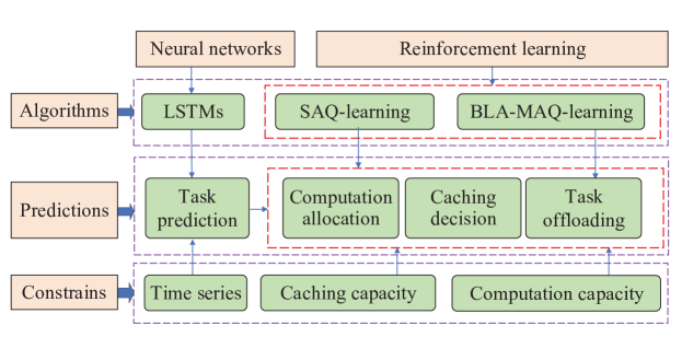
The structure of the cache-aided NOME MEC networks is depicted in Fig. 2. Firstly, we predict the task popularity utilizing the LSTMs. Then, based on the predicted task popularity, we formulate a long-term resource allocation problem, which is solved utilizing a single-agent Q-learning (SAQ-learning) algorithm. Finally, we proposed a BLA based MAQ-learning algorithm for the long-term task offloading problem.

III LSTMs for Task Popularity Prediction

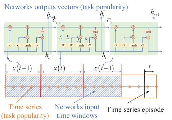
Generally, task popularity information can be revealed by direct measurements in real time or by computational estimation of historical data. However, the above techniques suffer from some technical and mercantile issues. Therefore, we predict task popularity from the previously collected data instead of measuring it directly. To predict task popularity, we need to model the map between the historical task popularity and task popularity in the future, which can be used as input sequences and output sequences, respectively. We adopt the widely used LSTMs model to determine the mapping. LSTMs have been widely used for time series prediction like text, speech, audio, etc, to ensure the persistence in learning, by connecting the offline historical data and online data. In our task popularity prediction, we formulate the task popularity as a time series, because it changes in different time slots. In practical situations, we are able to collect the series in a long-term storage. Based on the storage, we are capable of predicting the task popularity in the near future. Since the task popularity evolves over time, we define a dynamic series 𝐗𝐭=[x(1),x(2),x(Tp)]subscript𝐗𝐭𝑥1𝑥2𝑥subscript𝑇𝑝{\bf{X_{t}}}=\left[{x\left(1\right),x\left(2\right),\cdots x\left({{T_{p}}}\right)}\right], where x(t)=[Pr(1),Pr(2),Pr(Ts)]𝑥𝑡Pr1Pr2Prsubscript𝑇𝑠x\left(t\right)=\left[{\Pr\left(1\right),\Pr\left(2\right),\cdots\Pr\left({{T_{s}}}\right)}\right] denotes a series of task popularity. We assume that time slots are discretized and collect Tpsubscript𝑇𝑝T_{p} samples of popularity. The input and output of the LSTMs model are presented in Fig. 3. The goal is to predict xt+1subscript𝑥𝑡1{x_{t+1}} based on our current and past observations [x(1),x(2),x(Tp)]𝑥1𝑥2𝑥subscript𝑇𝑝\left[{x\left(1\right),x\left(2\right),\cdots x\left({{T_{p}}}\right)}\right]. Assuming that the output of the network is denoted as 𝐱^𝐭subscript^𝐱𝐭{\bf{\widehat{x}_{t}}}, and the observed real task popularity is 𝐱𝐭subscript𝐱𝐭{\bf{x_{t}}}. Our goal is to minimize 𝐭=𝟏𝐓𝐋(𝐱𝐭,𝐱^𝐭)=𝐭=𝟏𝐓(𝐱𝐭𝐱^𝐭)𝟐superscriptsubscript𝐭1𝐓𝐋subscript𝐱𝐭subscript^𝐱𝐭superscriptsubscript𝐭1𝐓superscriptsubscript𝐱𝐭subscript^𝐱𝐭2{\bf\sum\nolimits_{t=1}^{T}{L\left({{x_{t}},{{\widehat{x}}_{t}}}\right)}=\sum\nolimits_{t=1}^{T}{{{\left({{x_{t}}-{{\widehat{x}}_{t}}}\right)}^{2}}}}.

Refer to caption
Figure 3: Flow chart of LSTMs for task popularity prediction.

The core component of LSTMs to implement the above property is the memory cell state integrated with serval gates to filter different information sequences. This paper follows a similar approach for constructing LSTMs as [39]. There are several types of gates in LSTMs, which are described below:

Forget gate: the forget gate decides whether to retain the information by the sigmoid function. The input of the forget gate is 𝐱𝐭subscript𝐱𝐭{\bf{x_{t}}} and 𝐡𝐭𝟏subscript𝐡𝐭1{\bf{h_{t-1}}}, while the output is a number between 00 and 111 for each number in the memory cell state 𝐂𝐭𝟏subscript𝐂𝐭1{\bf C_{t-1}}.

𝐟𝐭=σ(𝐖𝐟[𝐡𝐭𝟏,𝐱𝐭]+𝐛𝐟),subscript𝐟𝐭𝜎subscript𝐖𝐟subscript𝐡𝐭1subscript𝐱𝐭subscript𝐛𝐟{\bf{f_{t}}=\sigma\left({{W_{f}}\left[{{h_{t-1}},{x_{t}}}\right]+{b_{f}}}\right)}, (11)

where 𝐱𝐭subscript𝐱𝐭{\bf{{x_{t}}}} and 𝐡𝐭𝟏subscript𝐡𝐭1{\bf{{h_{t-1}}}} denote the input of the forget gate. 𝐖𝐟subscript𝐖𝐟{\bf{{W_{f}}}} and 𝐛𝐟subscript𝐛𝐟{\bf{{b_{f}}}} denotes the weights and bias of the layer, respectively.

Input gate: the input gate decides which information to be committed to memory. The function of input gate is achieved by a sigmoid gate and a tanh gate given below:

𝐢𝐭=σ(𝐖𝐢[𝐡𝐭𝟏,𝐱𝐭]+𝐛𝐢),subscript𝐢𝐭𝜎subscript𝐖𝐢subscript𝐡𝐭1subscript𝐱𝐭subscript𝐛𝐢{\bf{i_{t}}=\sigma\left({{W_{i}}\left[{{h_{t-1}},{x_{t}}}\right]+{b_{i}}}\right)}, (12)
𝐝𝐭=tanh(𝐖𝐂[𝐡𝐭𝟏,𝐱𝐭]+𝐛𝐂).subscript𝐝𝐭subscript𝐖𝐂subscript𝐡𝐭1subscript𝐱𝐭subscript𝐛𝐂{\bf{d_{t}}=\tanh\left({{W_{C}}\left[{{h_{t-1}},{x_{t}}}\right]+{b_{C}}}\right)}. (13)

where 𝐖𝐢subscript𝐖𝐢{\bf{W_{i}}} and 𝐖𝐂subscript𝐖𝐂{\bf W_{C}} denote the weights of the layers while 𝐛𝐢subscript𝐛𝐢\bf{b_{i}} and 𝐛𝐂subscript𝐛𝐂\bf{b_{C}} represent the bias of the layers.

Output gate: The output gate decides which information to output. Based on Eq. (11), (12), (13), we obtain the new memory cell state 𝐂𝐭subscript𝐂𝐭{\bf C_{t}}. The output gate also contains two layers (i.e., a sigmoid layer and a tanh layer).

Algorithm 1 LSTMs based task popularity prediction.
1:  Stage One: Back propagation through time (BPTT) training
1:  Time interval Tssubscript𝑇𝑠T_{s}, Training data: task popularity [Pr(1),Pr(2),Pr(Tp)]Pr1Pr2Prsubscript𝑇𝑝\left[{\Pr\left(1\right),\Pr\left(2\right),\cdots\Pr\left({{T_{p}}}\right)}\right].
2:  Randomly initialize weight matrix 𝐖𝐟,𝐖𝐢,𝐖𝐂,𝐖𝐨subscript𝐖𝐟subscript𝐖𝐢subscript𝐖𝐂subscript𝐖𝐨{\bf{W_{f}},{W_{i}},{W_{C}},{W_{o}}} and bias 𝐛𝐟,𝐛𝐢,𝐛𝐂,𝐛𝐨subscript𝐛𝐟subscript𝐛𝐢subscript𝐛𝐂subscript𝐛𝐨{\bf{b_{f}},{b_{i}},{b_{C}},{b_{o}}} in the hidden layers.
3:  for each episode do
4:     Choose input x(t)𝑥𝑡x\left(t\right) from training set; 
5:     Forward propagation algorithm: calculate the output of the layers 𝐡𝐭subscript𝐡𝐭{\bf{h_{t}}}
6:     Calculate loss function 𝐭=𝟏𝐓𝐋(𝐱𝐭,𝐱^𝐭)superscriptsubscript𝐭1𝐓𝐋subscript𝐱𝐭subscript^𝐱𝐭\sum\nolimits_{{\bf{t}}={\bf{1}}}^{\bf{T}}{{\bf{L}}\left({{{\bf{x}}_{\bf{t}}},{{{\bf{\hat{x}}}}_{\bf{t}}}}\right)}
7:     BPTT algorithm: adjust the weights 𝐖𝐟,𝐖𝐢,𝐖𝐂,𝐖𝐨subscript𝐖𝐟subscript𝐖𝐢subscript𝐖𝐂subscript𝐖𝐨{\bf{W_{f}},{W_{i}},{W_{C}},{W_{o}}} and bias 𝐛𝐟,𝐛𝐢,𝐛𝐂,𝐛𝐨subscript𝐛𝐟subscript𝐛𝐢subscript𝐛𝐂subscript𝐛𝐨{\bf{b_{f}},{b_{i}},{b_{C}},{b_{o}}} according to the loss function; 
8:  end for
8:  Weights 𝐖𝐟,𝐖𝐢,𝐖𝐂,𝐖𝐨subscript𝐖𝐟subscript𝐖𝐢subscript𝐖𝐂subscript𝐖𝐨{\bf{W_{f}},{W_{i}},{W_{C}},{W_{o}}} and bias 𝐛𝐟,𝐛𝐢,𝐛𝐂,𝐛𝐨subscript𝐛𝐟subscript𝐛𝐢subscript𝐛𝐂subscript𝐛𝐨{\bf{b_{f}},{b_{i}},{b_{C}},{b_{o}}} of the network. 
9:  Stage Two: Testing
9:  Time interval Tssubscript𝑇𝑠T_{s}, Testing data: task popularity, Parameters of s: weights 𝐖𝐟,𝐖𝐢,𝐖𝐂,𝐖𝐨subscript𝐖𝐟subscript𝐖𝐢subscript𝐖𝐂subscript𝐖𝐨{\bf{W_{f}},{W_{i}},{W_{C}},{W_{o}}} and bias 𝐛𝐟,𝐛𝐢,𝐛𝐂,𝐛𝐨subscript𝐛𝐟subscript𝐛𝐢subscript𝐛𝐂subscript𝐛𝐨{\bf{b_{f}},{b_{i}},{b_{C}},{b_{o}}} of the network, number of epochs.
10:  for each episode do
11:     Choose input 𝐗𝐗{\bf{X}} from testing set; 
12:     Forward propagation: calculate the output of the layers 𝐡𝐭subscript𝐡𝐭{\bf{h_{t}}}
13:     Calculate loss function 𝐭=𝟏𝐓𝐋(𝐱𝐭,𝐱^𝐭)superscriptsubscript𝐭1𝐓𝐋subscript𝐱𝐭subscript^𝐱𝐭\sum\nolimits_{{\bf{t}}={\bf{1}}}^{\bf{T}}{{\bf{L}}\left({{{\bf{x}}_{\bf{t}}},{{{\bf{\hat{x}}}}_{\bf{t}}}}\right)}
14:  end for
14:  Task popularity in the next time slot [Pr(Tp+1),Pr(Tp+2),Pr(Tp+Ts)]Prsubscript𝑇𝑝1Prsubscript𝑇𝑝2Prsubscript𝑇𝑝subscript𝑇𝑠\left[{\Pr\left({{T_{p}}+1}\right),\Pr\left({{T_{p}}+2}\right),\cdots\Pr\left({{T_{p}}+{T_{s}}}\right)}\right].
𝐂𝐭=𝐟𝐭𝐂𝐭𝟏+𝐢𝐭𝐝𝐭,subscript𝐂𝐭subscript𝐟𝐭subscript𝐂𝐭1subscript𝐢𝐭subscript𝐝𝐭{\bf{C_{t}}={f_{t}}{C_{t-1}}+{i_{t}}{d_{t}},} (14)
𝐨𝐭=σ(𝐖𝐨[𝐡𝐭𝟏,𝐱𝐭]+𝐛𝐨),subscript𝐨𝐭𝜎subscript𝐖𝐨subscript𝐡𝐭1subscript𝐱𝐭subscript𝐛𝐨{\bf{o_{t}}=\sigma\left({{W_{o}}\left[{{h_{t-1}},{x_{t}}}\right]+{b_{o}}}\right),} (15)
𝐡𝐭=𝐨𝐭tanh(𝐂𝐭).subscript𝐡𝐭subscript𝐨𝐭subscript𝐂𝐭{\bf{h_{t}}={o_{t}}*\tanh\left({{C_{t}}}\right).} (16)

where 𝐂𝐭subscript𝐂𝐭{\bf{C_{t}}} is the state of the cell, 𝐨𝐭subscript𝐨𝐭{\bf{o_{t}}} is the combination of history output and input of this layer, 𝐡𝐭subscript𝐡𝐭{\bf{h_{t}}} is the output of the network, 𝐖𝐨subscript𝐖𝐨{\bf W_{o}} and 𝐛𝐨subscript𝐛𝐨{\bf b_{o}} denotes the weights and bias.

Remark 1.

The mobile users request different tasks in different time slots, thus the task popularity prediction is a time series prediction problem. The balance ability between historical information and instantaneous information of the proposed LSTMs makes it capable of predicting the task popularity in the cache-aided NOMA MEC networks.

Given the output of the network 𝐡𝐭subscript𝐡𝐭{\bf{h_{t}}}, the estimated output is obtained as

𝐱^𝐭=𝐰𝐭𝐡𝐭=𝐰𝐭𝐨𝐭tanh(𝐂𝐭),subscript^𝐱𝐭subscript𝐰𝐭subscript𝐡𝐭absentsubscript𝐰𝐭subscript𝐨𝐭subscript𝐂𝐭\begin{array}[]{l}\bf{\widehat{x}_{t}}={w_{t}}{h_{t}}\\ {\kern 1.0pt}{\kern 1.0pt}{\kern 1.0pt}{\kern 1.0pt}{\kern 1.0pt}{\kern 1.0pt}{\kern 1.0pt}{\kern 1.0pt}{\kern 1.0pt}{\kern 1.0pt}{\kern 1.0pt}{\kern 1.0pt}{\kern 1.0pt}={\bf{w_{t}}{o_{t}}*\tanh\left({{C_{t}}}\right)},\end{array} (17)

where 𝐰𝐭subscript𝐰𝐭{\bf w_{t}} is the regression coefficient.

To obtain the corresponding parameters above, we introduce the real-time recurrent learning (RTRL) algorithm [40], which enjoys low complexity for our proposed task popularity prediction scenario. For the weight vector 𝐰𝐭subscript𝐰𝐭\bf{w_{t}} in Eq. (17)

𝐰𝐭+𝟏subscript𝐰𝐭1\displaystyle{\bf{w_{t+1}}} =𝐰𝐭μ𝐭𝐰𝐭𝐥(𝐱𝐭,𝐱^𝐭)absentsubscript𝐰𝐭subscript𝜇𝐭subscriptsubscript𝐰𝐭𝐥subscript𝐱𝐭subscript^𝐱𝐭\displaystyle={\bf{w_{t}}-{\mu_{t}}{\nabla_{{w_{t}}}}l\left({{x_{t}},{{\widehat{x}}_{t}}}\right)} (18)
=𝐰𝐭μ𝐭𝐰𝐭(𝐱𝐭𝐱^𝐭)𝟐\displaystyle={\bf{w_{t}}-{\mu_{t}}{\nabla_{{w_{t}}}}{\left({{x_{t}}-{{\widehat{x}}_{t}}}\right)^{2}}}
=𝐰𝐭+𝟐μ𝐭(𝐱𝐭𝐱^𝐭)𝐨𝐭tanh(𝐂𝐭),absentsubscript𝐰𝐭2subscript𝜇𝐭subscript𝐱𝐭subscript^𝐱𝐭subscript𝐨𝐭subscript𝐂𝐭\displaystyle={\bf{w_{t}}+2{\mu_{t}}\left({{x_{t}}-{{\widehat{x}}_{t}}}\right){o_{t}}\tanh\left({{C_{t}}}\right)},

where μ𝐭subscript𝜇𝐭{\bf{\mu_{t}}} represents the learning rate. We set μ𝐭=1/tsubscript𝜇𝐭1/𝑡{\bf{\mu_{t}}={\raise 3.01385pt\hbox{$1$}\!\mathord{\left/{\vphantom{1t}}\right.\kern-1.2pt}\!\lower 3.01385pt\hbox{$t$}}}.

Proposition 1.

For each element wCsubscript𝑤𝐶w_{C} in 𝐖𝐂subscript𝐖𝐂{\bf{W_{C}}}, we update it as follows

𝐰𝐂=𝐰𝐂+𝟐μ𝐭(𝐱𝐭𝐱^𝐭)𝐰𝐭(𝐨𝐭tanh(𝐂𝐭))(𝐰𝐂).subscript𝐰𝐂subscript𝐰𝐂2subscript𝜇𝐭subscript𝐱𝐭subscript^𝐱𝐭subscript𝐰𝐭subscript𝐨𝐭subscript𝐂𝐭subscript𝐰𝐂{\bf{w_{C}}={w_{C}}+2{\mu_{t}}\left({{x_{t}}-{{\widehat{x}}_{t}}}\right){w_{t}}\frac{{\partial\left({{o_{t}}\tanh\left({{C_{t}}}\right)}\right)}}{{\partial\left({{w_{C}}}\right)}}}. (19)
Remark 2.

The partial derivative in Eq. (19) contains two parts: the first is the output 𝐨𝐭subscript𝐨𝐭{\bf{{o_{t}}}}, and the second part is the memory cell state tanh(𝐂𝐭)subscript𝐂𝐭{\bf\tanh\left({{C_{t}}}\right)}. We can implement Eq. (19) if we compute (𝐨𝐭)(𝐰𝐂)subscript𝐨𝐭subscript𝐰𝐂{\bf\frac{{\partial\left({{o_{t}}}\right)}}{{\partial\left({{w_{C}}}\right)}}} and (tanh(𝐂𝐭))(𝐰𝐂)subscript𝐂𝐭subscript𝐰𝐂{\bf\frac{{\partial\left({\tanh\left({{C_{t}}}\right)}\right)}}{{\partial\left({{w_{C}}}\right)}}}

Proof:

See Appendix A . ∎

IV Resource Allocation Problem Formulation and Proposed Approaches

IV-A Problem Formulation

Based on the predicted task popularity we obtained from Section III, we formulate the optimization problem for cache-aided NOMA MEC networks as in (20) below, in which, the objective function is the energy consumption given by Eq. (7). The parameters are the offloading decision vector, computation resources allocation vector and caching vector. The joint task offloading decision and resource allocation problem is formulated as follows:

(𝐏𝟏)minX,Y,Zt=1Ti=1Nu𝐄𝐢(t,xi(t),yi(t),zj(t)),𝐏𝟏subscriptmin𝑋𝑌𝑍superscriptsubscript𝑡1𝑇superscriptsubscript𝑖1subscript𝑁𝑢subscript𝐄𝐢𝑡subscript𝑥𝑖𝑡subscript𝑦𝑖𝑡subscript𝑧𝑗𝑡\displaystyle\left({{\bf{P1}}}\right)\mathop{{\rm{min}}}\limits_{X,Y,Z}\sum\limits_{t=1}^{T}{\sum\limits_{i=1}^{{N_{u}}}{{{\bf{E}}_{\bf{i}}}\left({t,{x_{i}}\left(t\right),{y_{i}}\left(t\right),{z_{j}}\left(t\right)}\right)}}, (20a)
s.t. C1:xi(t){0,1},i[1,Nu],t[1,T],:subscript𝐶1formulae-sequencesubscript𝑥𝑖𝑡01formulae-sequencefor-all𝑖1subscript𝑁𝑢𝑡1𝑇\displaystyle C_{1}:\;{x_{i}}\left(t\right)\in\left\{{0,1}\right\},\forall i\in\left[{1,{N_{u}}}\right],t\in\left[{1,T}\right], (20b)
C2:yi(t)[0,1],i[1,Nu],t[1,T],:subscript𝐶2formulae-sequencesubscript𝑦𝑖𝑡01formulae-sequencefor-all𝑖1subscript𝑁𝑢𝑡1𝑇\displaystyle C_{2}:\;{y_{i}}\left(t\right)\in\left[{0,1}\right],\forall i\in\left[{1,{N_{u}}}\right],t\in\left[{1,T}\right], (20c)
C3:zj(t){0,1},j[1,Nt],t[1,T],:subscript𝐶3formulae-sequencesubscript𝑧𝑗𝑡01formulae-sequencefor-all𝑗1subscript𝑁𝑡𝑡1𝑇\displaystyle C_{3}:\;{z_{j}}\left(t\right)\in\left\{{0,1}\right\},\forall j\in\left[{1,{N_{t}}}\right],t\in\left[{1,T}\right], (20d)
C4:i=1Nuyi(t)=1,t[1,T],:subscript𝐶4formulae-sequencesuperscriptsubscript𝑖1subscript𝑁𝑢subscript𝑦𝑖𝑡1for-all𝑡1𝑇\displaystyle C_{4}:\;\sum\limits_{i=1}^{{N_{u}}}{{y_{i}}}\left(t\right)=1,\forall t\in\left[{1,T}\right], (20e)
C5:j=1Ntzj(t)Ccache,t[1,T],:subscript𝐶5formulae-sequencesuperscriptsubscript𝑗1subscript𝑁𝑡subscript𝑧𝑗𝑡subscript𝐶cachefor-all𝑡1𝑇\displaystyle C_{5}:\;\sum\limits_{j=1}^{N_{t}}{{z_{j}}\left(t\right)}\leq{C_{{\rm{cache}}}},\forall t\in\left[{1,T}\right], (20f)
C6:𝐓𝐣𝐨(𝐭)T,j[1,Nt],t[1,T].:subscript𝐶6formulae-sequencesuperscriptsubscript𝐓𝐣𝐨𝐭𝑇formulae-sequencefor-all𝑗1subscript𝑁𝑡𝑡1𝑇\displaystyle C_{6}:\;{\bf T_{j}^{o}\left(t\right)}\leq T,\forall j\in\left[{1,{N_{t}}}\right],t\in\left[{1,T}\right]. (20g)
where 𝐄𝐢(t,xi,yj,zj)subscript𝐄𝐢𝑡subscript𝑥𝑖subscript𝑦𝑗subscript𝑧𝑗{{\bf{E}}_{\bf{i}}}\left({t,{x_{i}},{y_{j}},{z_{j}}}\right) denotes the energy consumption for computing task j𝑗j given in Eq. (7), xi(t)subscript𝑥𝑖𝑡{x_{i}}\left(t\right) denotes the offloading decision of user i𝑖i at time t𝑡t, and yi(t)subscript𝑦𝑖𝑡{y_{i}}\left(t\right) denotes the computing speed that the AP allocates to user i𝑖i at time t𝑡t. The variable zj(t)subscript𝑧𝑗𝑡{z_{j}}\left(t\right) denotes the task caching decision of task j𝑗j at time t𝑡t. Eq. (20e) guarantees that the task computing resource allocation is valid. While Eq. (20f) guarantees that the task computation results cached do not exceed the caching capacity of the AP. Finally, Eq. (20g) guarantees the time constraint.
Remark 3.

The formulated problem is a long-term minimization problem. Consequently, in order to solve it, we need to design a long-term policy, which instantaneously gives the optimal offloading decision vector, computation resources allocation vector and caching vector at different time slots.

IV-B SAQ-learning Solution for Cache-aided NOMA MEC

In this section, a single-agent Q-learning (SAQ-learning) algorithm is proposed for the formulated problem in Subsection IV-A. We reformulate the cache-aided NOMA MEC problem as a SAQ-learning model, which consists of three elements: states, actions, and rewards. The aim of this section is to devise a resource allocation policy πsuperscript𝜋{\pi^{*}} that is capable of quickly generating an optimal resource allocation action.

Qt(s,a)=(1γ)Qt1(s,a)historyQvalue+γlearningrate[rtobtainedreward+βdiscountfactormaxat+1Qt1(st+1,at+1)optimalQvalueinthenextstate].superscript𝑄𝑡𝑠𝑎1𝛾subscriptsuperscript𝑄𝑡1𝑠𝑎historyQvaluesubscript𝛾learningratedelimited-[]subscriptsubscript𝑟𝑡obtainedrewardsubscript𝛽discountfactorsubscriptsubscriptsubscript𝑎𝑡1superscript𝑄𝑡1subscript𝑠𝑡1subscript𝑎𝑡1optimalQvalueinthenextstate\displaystyle{Q^{t}}\left({s,a}\right)=\left({1-\gamma}\right)\underbrace{{Q^{t-1}}\left({s,a}\right)}_{{\rm history{\kern 1.0pt}{\kern 1.0pt}Q{\kern 1.0pt}{\kern 1.0pt}value}}+\underbrace{\gamma}_{{\rm learning{\kern 1.0pt}{\kern 1.0pt}rate}}\left[{\underbrace{{r_{t}}}_{{\rm obtained{\kern 1.0pt}{\kern 1.0pt}reward}}+\underbrace{\beta}_{{\rm discount{\kern 1.0pt}{\kern 1.0pt}factor}}\underbrace{\mathop{\max}\limits_{{a_{t+1}}}{Q^{t-1}}\left({{s_{t+1}},{a_{t+1}}}\right)}_{{\rm optimal{\kern 1.0pt}{\kern 1.0pt}Q{\kern 1.0pt}{\kern 1.0pt}value{\kern 1.0pt}{\kern 1.0pt}{\kern 1.0pt}{\kern 1.0pt}in{\kern 1.0pt}{\kern 1.0pt}the{\kern 1.0pt}{\kern 1.0pt}next{\kern 1.0pt}{\kern 1.0pt}state}}}\right]. (21)
Definition 1.

A SAQ-learning model is a tuple 𝒮,𝒜,𝒮𝒜\left\langle{{\cal S},{\cal A},{\cal R}}\right\rangle. The definitions of the three parameters are given below.

  • State space (𝒮𝒮\mathcal{S}): A finite set of states of the agent; We assume that all the users are controlled by a central agent, the state of agent is denoted as st=i=1Nu𝐄𝐢(t,xi(t),yi(t),zj(t))subscript𝑠𝑡superscriptsubscript𝑖1subscript𝑁𝑢subscript𝐄𝐢𝑡subscript𝑥𝑖𝑡subscript𝑦𝑖𝑡subscript𝑧𝑗𝑡{s_{t}}=\sum\limits_{i=1}^{{N_{u}}}{{{\bf{E}}_{\bf{i}}}\left({t,{x_{i}}\left(t\right),{y_{i}}\left(t\right),{z_{j}}\left(t\right)}\right)}. The state is the energy consumption of the network in time slot t𝑡t.

  • Action space (𝒜𝒜\mathcal{A}): A finite set of actions. The action of the central agent is defined as at=[a1(t),a2(t),a3(t)]subscript𝑎𝑡subscript𝑎1𝑡subscript𝑎2𝑡subscript𝑎3𝑡{a_{t}}=\left[{{a_{1}}\left(t\right),{a_{2}}\left(t\right),{a_{3}}\left(t\right)}\right], where, the first part a1(t)=[x1(t),,xNu(t)]subscript𝑎1𝑡subscript𝑥1𝑡subscript𝑥subscript𝑁𝑢𝑡{a_{1}}\left(t\right)=\left[{{x_{1}}\left(t\right),\cdots,{x_{N_{u}}}\left(t\right)}\right] is the task offloading vector of the users. The second part a2(t)=[f1(t),,fNu(t)]subscript𝑎2𝑡subscript𝑓1𝑡subscript𝑓subscript𝑁𝑢𝑡{a_{2}}\left(t\right)=\left[{{f_{1}}\left(t\right),\cdots,{f_{N_{u}}}\left(t\right)}\right] contains the computing speed allocation from the AP to all users. The last part a3(t)=[c1(t),,cNu(t)]subscript𝑎3𝑡subscript𝑐1𝑡subscript𝑐subscript𝑁𝑢𝑡{a_{3}}\left(t\right)=\left[{{c_{1}}\left(t\right),\cdots,{c_{N_{u}}}\left(t\right)}\right] represents the cache decision of the AP.

  • Reward function ({\cal R}): The reward function is the key to solve (𝐏𝟏)𝐏𝟏\left({{\bf{P1}}}\right) by utilizing the SAQ-learning model. The objective of SAQ-learning is to maximize the expected long-term reward, also known as the state-value function given by:

    Vπ(s)subscript𝑉𝜋𝑠\displaystyle{V_{\pi}}(s) =𝔼π[t=0γtrt|s0=s]absentsubscript𝔼𝜋delimited-[]conditionalsuperscriptsubscript𝑡0superscript𝛾𝑡subscript𝑟𝑡subscript𝑠0𝑠\displaystyle={\mathbb{E}_{\pi}}\left[{\sum\limits_{t=0}^{\infty}{{\gamma^{t}}{r_{t}}\left|{s_{0}={s}}\right.}}\right] (22)
    =𝔼π[r0+γE[γr1+γ2r2+]|s0=s]absentsubscript𝔼𝜋delimited-[]subscript𝑟0conditional𝛾𝐸delimited-[]𝛾subscript𝑟1superscript𝛾2subscript𝑟2subscript𝑠0𝑠\displaystyle={\mathbb{E}_{\pi}}\left[{{r_{0}}+\gamma E\left[{\gamma{r_{1}}+{\gamma^{2}}{r_{2}}+...}\right]\left|{s_{0}={s}}\right.}\right]
    =𝔼π[r(s|s0,a)+γVπ(s)|s0=s].absentsubscript𝔼𝜋delimited-[]𝑟conditionalsuperscript𝑠subscript𝑠0𝑎conditional𝛾superscript𝑉𝜋superscript𝑠subscript𝑠0𝑠\displaystyle={\mathbb{E}_{\pi}}\left[{r\left({s^{\prime}\left|{{s_{0}},a}\right.}\right)+\gamma{V^{\pi}}(s^{\prime})\left|{s_{0}={s}}\right.}\right].

    where γ𝛾\gamma represents the learning rate and rtsubscript𝑟𝑡{{r_{t}}} denotes the reward that the agents obtain in time slot t𝑡t. In order to minimize the energy consumption in (𝐏𝟏)𝐏𝟏\left({{\bf{P1}}}\right), we define the reward function as rt=i=1Nu𝐄𝐢(t1,st1)i=1Nu𝐄𝐢(t,st)subscript𝑟𝑡superscriptsubscript𝑖1subscript𝑁𝑢subscript𝐄𝐢𝑡1subscript𝑠𝑡1superscriptsubscript𝑖1subscript𝑁𝑢subscript𝐄𝐢𝑡subscript𝑠𝑡{r_{t}}=\sum\nolimits_{i=1}^{{N_{u}}}{{{\bf{E}}_{\bf{i}}}\left({t-1,{s_{t-1}}}\right)}-\sum\nolimits_{i=1}^{{N_{u}}}{{{\bf{E}}_{\bf{i}}}\left({t,{s_{t}}}\right)}.

  • Action value function (Qπ(s,a)superscript𝑄𝜋𝑠𝑎{Q^{\pi}}(s,a)): The long-run average reward is the payoff of an infinite path where every state-action pair is assigned a real-valued reward.

    Qπ(s,a)=𝔼π[i=0γiri|s=s0,a=a0].superscript𝑄𝜋𝑠𝑎subscript𝔼𝜋delimited-[]formulae-sequenceconditionalsuperscriptsubscript𝑖0superscript𝛾𝑖subscript𝑟𝑖𝑠subscript𝑠0𝑎subscript𝑎0{Q^{\pi}}(s,a)={\mathbb{E}_{\pi}}\left[{\sum\limits_{i=0}^{\infty}{{\gamma^{i}}{r_{i}}\left|{s={s_{0}},a={a_{0}}}\right.}}\right]. (23)
  • A policy π𝜋\pi is a distribution over actions given states,

    π(a|s)=P[At=a|St=s],𝜋conditional𝑎𝑠𝑃delimited-[]subscript𝐴𝑡conditional𝑎subscript𝑆𝑡𝑠\pi\left({a|s}\right)=P\left[{{A_{t}}=a|{S_{t}}=s}\right], (24)

    where a policy fully defines the behaviour of an agent.

Therefore, the optimal policy is given by

π(s)=argminαVπ(s),sS,formulae-sequencesuperscript𝜋𝑠subscript𝛼subscript𝑉𝜋𝑠for-all𝑠𝑆{\pi^{*}}\left(s\right)=\mathop{\arg\min}\limits_{\alpha}{V_{\pi}}(s),\forall s\in S, (25)

which finds an optimal policy (i.e., a set of actions) to maximize the long-run average reward.

TABLE II: Q-table of Q-learning Algorithm
a1subscript𝑎1{a_{1}} a2subscript𝑎2{a_{2}} aN2subscript𝑎subscript𝑁2{a_{N_{2}}}
s1subscript𝑠1{s_{1}} Q1,1(s1,a1)superscript𝑄11subscript𝑠1subscript𝑎1{Q^{1,1}}\left({{s_{1}},{a_{1}}}\right) Q1,2(s1,a2)superscript𝑄12subscript𝑠1subscript𝑎2{Q^{1,2}}\left({{s_{1}},{a_{2}}}\right) Q1,N2(s1,aN2)superscript𝑄1subscript𝑁2subscript𝑠1subscript𝑎subscript𝑁2{Q^{1,N_{2}}}\left({{s_{1}},{a_{N_{2}}}}\right)
s2subscript𝑠2{s_{2}} Q2,1(s2,a1)superscript𝑄21subscript𝑠2subscript𝑎1{Q^{2,1}}\left({{s_{2}},{a_{1}}}\right) Q2,2(s2,a2)superscript𝑄22subscript𝑠2subscript𝑎2{Q^{2,2}}\left({{s_{2}},{a_{2}}}\right) Q2,N2(s2,aN2)superscript𝑄2subscript𝑁2subscript𝑠2subscript𝑎subscript𝑁2{Q^{2,N_{2}}}\left({{s_{2}},{a_{N_{2}}}}\right)
sN1subscript𝑠subscript𝑁1s_{N_{1}} QN1,1(sN1,a1)superscript𝑄subscript𝑁11subscript𝑠subscript𝑁1subscript𝑎1{Q^{{N_{1}},1}}\left({{s_{{N_{1}}}},{a_{1}}}\right) QN1,2(sN1,a2)superscript𝑄subscript𝑁12subscript𝑠subscript𝑁1subscript𝑎2{Q^{{N_{1}},2}}\left({{s_{{N_{1}}}},{a_{2}}}\right) QN1,N2(sN1,aN2)superscript𝑄subscript𝑁1subscript𝑁2subscript𝑠subscript𝑁1subscript𝑎subscript𝑁2{Q^{{N_{1}},N_{2}}}\left({{s_{{N_{1}}}},{a_{N_{2}}}}\right)

According to [41], the optimal state-value function Vπ(s)superscript𝑉𝜋𝑠{V^{\pi}}\left(s\right) can be achieved by solving the Bellman’s optimality equation.

Remark 4.

The optimal state-value function Vπ(s)superscript𝑉𝜋𝑠{V^{\pi}}\left(s\right) satisfies the Bellman’s optimality equation, which is given by

Vπ(s)=minaA{(1γ)p(x,y)+γsSPr{s|s,a}V(s)}.superscript𝑉𝜋𝑠subscript𝑎𝐴1𝛾𝑝𝑥𝑦𝛾subscriptsuperscript𝑠𝑆Prconditionalsuperscript𝑠𝑠𝑎𝑉superscript𝑠{V^{\pi}}\left(s\right)=\mathop{\min}\limits_{a\in A}\left\{{\left({1-\gamma}\right)p\left({x,y}\right)+\gamma\sum\limits_{s^{\prime}\in S}{\Pr\left\{{s^{\prime}|s,a}\right\}V\left({s^{\prime}}\right)}}\right\}. (26)

In order to solve this problem, Bellman’s equations and backward induction are used. We develop a SAQ-learning based resource allocation algorithm for cache-aided NOMA MEC system. In SAQ-learning, the Q value Qt(s,a)superscript𝑄𝑡𝑠𝑎{Q^{t}}\left({s,a}\right) at time slot t𝑡t is updated as in Eq. (21). The SAQ-learning algorithm for cache-aided NOMA MEC includes two cycles: the first cycle in each episode obtains the optimal policy, while the second cycle in each step executes the policy in each step. The central agent has to decide all the actions from the first to the last time slot to minimize the total long-term energy consumption. The details of the SAQ-learning are presented in our previous work [36], and are omitted here due to space limitations. The size of the Q-table is shown in Table II, in which N1=2NuNNfsubscript𝑁1superscript2subscript𝑁𝑢superscript𝑁subscript𝑁𝑓{N_{1}}={2^{{N_{u}}}}{N^{{N_{f}}}}, N2=2NuNfsubscript𝑁22subscript𝑁𝑢subscript𝑁𝑓{N_{2}}=2{{N_{u}}}{{N_{f}}}, where Nusubscript𝑁𝑢N_{u} represent the number of users and, Nfsubscript𝑁𝑓N_{f} denotes the number of slices the computing resources are sliced into.

IV-C BLA-MAQ-learning Solution for Task Offloading

To reduce the dimension of state space and action space of the agent, which reduce the performance of learning [36], we propose a distributed RL algorithm, i.e., MAQ-learning algorithm, for task offloading. In MAQ-learning, the users operate cooperatively as distributed agents to decide whether to offload the computation tasks to the server or not.

Definition 2.

A MAQ-learning model is a tuple 𝒮,𝒜,𝒮𝒜\left\langle{{\cal S},{\cal A},{\cal R}}\right\rangle. The definition of the parameters adopted in MAQ-learning are given below.

  • State (𝒮𝒮\mathcal{S}): We assume that all the users are set as agents, the state of agent i𝑖i is denoted as sti=𝐄𝐢(t)superscriptsubscript𝑠𝑡𝑖subscript𝐄𝐢𝑡s_{t}^{i}={{\bf{E}}_{\bf{i}}}\left(t\right). The state is the energy consumption of computing of the task that the user requests.

  • Action (𝒜𝒜\mathcal{A}): The action of the agent i𝑖i is defined as ati[0,1]superscriptsubscript𝑎𝑡𝑖01a_{t}^{i}\in\left[{0,1}\right], where ati=1superscriptsubscript𝑎𝑡𝑖1a_{t}^{i}{\rm{=1}} implies that the task is computed locally while ati=0superscriptsubscript𝑎𝑡𝑖0a_{t}^{i}{\rm{=0}} implies that the task is offloaded to the AP for computing.

  • Reward function ({\cal R}): The local reward function of the central agent is defined as rti=𝐄𝐢(t1,st1i)𝐄𝐢(t,sti)superscriptsubscript𝑟𝑡𝑖subscript𝐄𝐢𝑡1superscriptsubscript𝑠𝑡1𝑖subscript𝐄𝐢𝑡superscriptsubscript𝑠𝑡𝑖r_{t}^{i}={{\bf{E}}_{\bf{i}}}\left({t-1,s_{t-1}^{i}}\right)-{{\bf{E}}_{\bf{i}}}\left({t,s_{t}^{i}}\right).

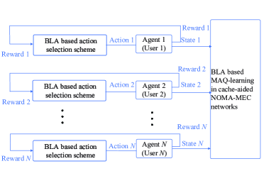
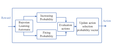
Different from SAQ-learning, in the MAQ-learning case, three cycles are looped over. Apart from the two cycles in SAQ-learning, one more loop for the agents is added, to cooperatively decide the actions, as shown in Fig. 4. The action selection scheme (i.e., how the action is selected during the learning process) is the core issue in the RL algorithm, which is utilized to balance the exploration and exploitation and avoiding over-fitting. In conventional RL algorithms, ϵitalic-ϵ\epsilon-greedy exploration is adopted. However, the selection mechanism of ϵitalic-ϵ\epsilon-greedy exploration is based on a random mechanism. In order to overcome this drawback, we apply Bayesian learning automata (BLA) for action selection, because BLA is capable of choosing the optimal action for two action case [42].
Refer to caption
(a) Bayesian learning automata based action selection scheme.
Refer to caption
(b) BLA-MAQL for cache-aided NOMA-MEC networks.
Figure 4: An illustration of Bayesian learning automata based multi-agent Q-learning in cache-aided NOMA-MEC networks.

A BLA is an adaptive decision-making unit which learns the optimal action from a set of actions offered by the environment it operates in. Essentially, there are two Beta distributions in the BLA based action selection scheme. In our MEC scenario, we assume that the computation task is computed locally as Arm 1, while the task is offloaded to MEC server for computing as Arm 2. The heart of BLA is the beta distribution, whose probability density function is:

f(x;α,β)=xα1(1x)β101uα1(1u)β1𝑑u,x[0,1],𝑓𝑥𝛼𝛽superscript𝑥𝛼1superscript1𝑥𝛽1superscriptsubscript01superscript𝑢𝛼1superscript1𝑢𝛽1differential-d𝑢𝑥01missing-subexpressionmissing-subexpressionmissing-subexpressionmissing-subexpressionmissing-subexpressionmissing-subexpressionmissing-subexpressionmissing-subexpressionmissing-subexpressionmissing-subexpressionmissing-subexpressionmissing-subexpressionmissing-subexpressionmissing-subexpressionmissing-subexpressionmissing-subexpressionmissing-subexpressionmissing-subexpression\begin{array}[]{*{20}{c}}{f\left({x;\alpha,\beta}\right)=\frac{{{x^{\alpha-1}}{{\left({1-x}\right)}^{\beta-1}}}}{{\int_{0}^{1}{{u^{\alpha-1}}{{\left({1-u}\right)}^{\beta-1}}du}}},}&{x\in\left[{0,1}\right]}\end{array}, (27)

where α𝛼\alpha and β𝛽\beta are the parameters of beta distribution and the corresponding cumulative distribution function is:

F(x;α,β)=0xtα1(1t)β1𝑑t01uα1(1u)β1𝑑u,x[0,1].𝐹𝑥𝛼𝛽superscriptsubscript0𝑥superscript𝑡𝛼1superscript1𝑡𝛽1differential-d𝑡superscriptsubscript01superscript𝑢𝛼1superscript1𝑢𝛽1differential-d𝑢𝑥01missing-subexpressionmissing-subexpressionmissing-subexpressionmissing-subexpressionmissing-subexpressionmissing-subexpressionmissing-subexpressionmissing-subexpressionmissing-subexpressionmissing-subexpressionmissing-subexpressionmissing-subexpressionmissing-subexpressionmissing-subexpressionmissing-subexpressionmissing-subexpressionmissing-subexpressionmissing-subexpression\begin{array}[]{*{20}{c}}{F\left({x;\alpha,\beta}\right)=\frac{{\int_{0}^{x}{{t^{\alpha-1}}{{\left({1-t}\right)}^{\beta-1}}dt}}}{{\int_{0}^{1}{{u^{\alpha-1}}{{\left({1-u}\right)}^{\beta-1}}du}}},}&{x\in\left[{0,1}\right]}\end{array}. (28)

BLA uses the beta distribution for two purposes. Firstly, the beta distribution is used to provide a Bayesian estimation of the reward probabilities associated with each action of Q-learning. Secondly, a novel feature of BLA is that it uses the beta distribution as the basis for a randomized action selection mechanism. The state of user i𝑖i at time slot n𝑛n is sin=(α1n,β1n,α2n,β2n)superscriptsubscript𝑠𝑖𝑛superscriptsubscript𝛼1𝑛superscriptsubscript𝛽1𝑛superscriptsubscript𝛼2𝑛superscriptsubscript𝛽2𝑛s_{i}^{n}=\left({\alpha_{1}^{n},\beta_{1}^{n},\alpha_{2}^{n},\beta_{2}^{n}}\right), where (α1n,β1n)superscriptsubscript𝛼1𝑛superscriptsubscript𝛽1𝑛({\alpha_{1}^{n},\beta_{1}^{n}}) determines the parameter of the first Beta distribution, and (α2n,β2n)superscriptsubscript𝛼2𝑛superscriptsubscript𝛽2𝑛({\alpha_{2}^{n},\beta_{2}^{n}}) determines the parameter of the second Beta distribution. The action selection probability of Arm 1 (i.e., local computing) is given in Eq. (31). After taking the action, the parameters of the Beta distribution are updated as follows:

{αi=αi+1thefeedbackisarewardβi=βi+1thefeedbackisapenalty(i=1,2)casessubscript𝛼𝑖subscript𝛼𝑖1thefeedbackisarewardmissing-subexpressionmissing-subexpressionmissing-subexpressionmissing-subexpressionmissing-subexpressionmissing-subexpressionmissing-subexpressionmissing-subexpressionmissing-subexpressionmissing-subexpressionmissing-subexpressionmissing-subexpressionmissing-subexpressionmissing-subexpressionmissing-subexpressionmissing-subexpressionmissing-subexpressionmissing-subexpressionsubscript𝛽𝑖subscript𝛽𝑖1thefeedbackisapenaltymissing-subexpressionmissing-subexpressionmissing-subexpressionmissing-subexpressionmissing-subexpressionmissing-subexpressionmissing-subexpressionmissing-subexpressionmissing-subexpressionmissing-subexpressionmissing-subexpressionmissing-subexpressionmissing-subexpressionmissing-subexpressionmissing-subexpressionmissing-subexpressionmissing-subexpressionmissing-subexpression𝑖12missing-subexpressionmissing-subexpressionmissing-subexpressionmissing-subexpressionmissing-subexpressionmissing-subexpressionmissing-subexpressionmissing-subexpressionmissing-subexpressionmissing-subexpressionmissing-subexpressionmissing-subexpressionmissing-subexpressionmissing-subexpressionmissing-subexpressionmissing-subexpressionmissing-subexpressionmissing-subexpressionmissing-subexpression\left\{{\begin{array}[]{*{20}{c}}{{\alpha_{i}}={\alpha_{i}}+1}&{{\rm the{\kern 1.0pt}{\kern 1.0pt}{\kern 1.0pt}{\kern 1.0pt}feedback{\kern 1.0pt}{\kern 1.0pt}{\kern 1.0pt}{\kern 1.0pt}is{\kern 1.0pt}{\kern 1.0pt}{\kern 1.0pt}{\kern 1.0pt}a{\kern 1.0pt}{\kern 1.0pt}{\kern 1.0pt}{\kern 1.0pt}reward}}\\ {{\beta_{i}}={\beta_{i}}+1}&{{\rm the{\kern 1.0pt}{\kern 1.0pt}{\kern 1.0pt}{\kern 1.0pt}feedback{\kern 1.0pt}{\kern 1.0pt}{\kern 1.0pt}{\kern 1.0pt}is{\kern 1.0pt}{\kern 1.0pt}{\kern 1.0pt}{\kern 1.0pt}a{\kern 1.0pt}{\kern 1.0pt}{\kern 1.0pt}{\kern 1.0pt}penalty}}\end{array}\begin{array}[]{*{20}{c}}{\left({i=1,2}\right)}\end{array}}\right. (29)

The BLA is briefly described as follows: The agent of BLA estimates the reward probability of every action utilizing two Beta distributions, denoted as 𝐁𝐞𝐭𝐚(α𝟏,β𝟏)𝐁𝐞𝐭𝐚subscript𝛼1subscript𝛽1{\bf Beta\left({{\alpha_{1}},{\beta_{1}}}\right)} and 𝐁𝐞𝐭𝐚(α𝟐,β𝟐)𝐁𝐞𝐭𝐚subscript𝛼2subscript𝛽2{\bf Beta\left({{\alpha_{2}},{\beta_{2}}}\right)}. During the learning process, two variables are generated according to the two Beta distributions, while the action of a higher variable is selected. Then, the reward of taking the chosen action is computed to update the parameters of the two Beta distribution.

The goal of RL is to find an optimal policy that maximize the expected sum of discounted return:

π=argmaxEππ[t=0T1γt+1r~(s~t,s~t+1)].superscript𝜋subscriptsuperscript𝐸𝜋𝜋delimited-[]superscriptsubscript𝑡0𝑇1superscript𝛾𝑡1~𝑟subscript~𝑠𝑡subscript~𝑠𝑡1{\pi^{*}}=\mathop{\arg\max{E^{\pi}}}\limits_{\pi}\left[{\sum\limits_{t=0}^{T-1}{{\gamma^{t+1}}\widetilde{r}\left({{{\widetilde{s}}_{t}},{{\widetilde{s}}_{t+1}}}\right)}}\right]. (30)
p1sBLAn=(α1n+β1n1)!(α2n+β2n1)!(α1n1)!(β1n1)!(α1n+β1n+α2n+β2n2)!×j=α2nα2n+β2n1(j+α1n1)!(β1n+α2n+β2nj2)!j!(α2n+β2n1j)!.superscriptsubscript𝑝1superscriptsubscript𝑠𝐵𝐿𝐴𝑛superscriptsubscript𝛼1𝑛superscriptsubscript𝛽1𝑛1superscriptsubscript𝛼2𝑛superscriptsubscript𝛽2𝑛1superscriptsubscript𝛼1𝑛1superscriptsubscript𝛽1𝑛1superscriptsubscript𝛼1𝑛superscriptsubscript𝛽1𝑛superscriptsubscript𝛼2𝑛superscriptsubscript𝛽2𝑛2superscriptsubscript𝑗superscriptsubscript𝛼2𝑛superscriptsubscript𝛼2𝑛superscriptsubscript𝛽2𝑛1𝑗superscriptsubscript𝛼1𝑛1superscriptsubscript𝛽1𝑛superscriptsubscript𝛼2𝑛superscriptsubscript𝛽2𝑛𝑗2𝑗superscriptsubscript𝛼2𝑛superscriptsubscript𝛽2𝑛1𝑗\displaystyle p_{1}^{s_{BLA}^{n}}=\frac{{\left({\alpha_{1}^{n}+\beta_{1}^{n}-1}\right)!\left({\alpha_{2}^{n}+\beta_{2}^{n}-1}\right)!}}{{\left({\alpha_{1}^{n}-1}\right)!\left({\beta_{1}^{n}-1}\right)!\left({\alpha_{1}^{n}+\beta_{1}^{n}+\alpha_{2}^{n}+\beta_{2}^{n}-2}\right)!}}\times\sum\limits_{j=\alpha_{2}^{n}}^{\alpha_{2}^{n}+\beta_{2}^{n}-1}{\frac{{\left({j+\alpha_{1}^{n}-1}\right)!\left({\beta_{1}^{n}+\alpha_{2}^{n}+\beta_{2}^{n}-j-2}\right)!}}{{j!\left({\alpha_{2}^{n}+\beta_{2}^{n}-1-j}\right)!}}}. (31)

The details of BLA based action selection can be found in Fig. 4(a). The first advantage of BLA compared with other learning automata (LA) algorithms is computational simplicity, achieved by relying implicitly on Bayesian reasoning principles. The second advantage of BLA is that for the two actions case, the action selected from BLA can be proven optimal. In our scenario, we assume that the computation task is computed locally as arm 1, while the task is offloaded to the MEC server to be computed as arm2. Given the state sBLAn=(α1n,β1n,α2n,β2n)superscriptsubscript𝑠𝐵𝐿𝐴𝑛superscriptsubscript𝛼1𝑛superscriptsubscript𝛽1𝑛superscriptsubscript𝛼2𝑛superscriptsubscript𝛽2𝑛s_{BLA}^{n}=\left({\alpha_{1}^{n},\beta_{1}^{n},\alpha_{2}^{n},\beta_{2}^{n}}\right), the action selection probability of local computing is given in Eq. (31).

P1(e1>e2)subscript𝑃1subscript𝑒1subscript𝑒2\displaystyle{P_{1}}\left({{e_{1}}>{e_{2}}}\right) =i=0α11B(α2+i,β1+β2)(β1+i)B(1+i,β1)B(α2,β2)absentsuperscriptsubscript𝑖0subscript𝛼11𝐵subscript𝛼2𝑖subscript𝛽1subscript𝛽2subscript𝛽1𝑖𝐵1𝑖subscript𝛽1𝐵subscript𝛼2subscript𝛽2\displaystyle=\sum\limits_{i=0}^{{\alpha_{1}}-1}{\frac{{B\left({{\alpha_{2}}+i,{\beta_{1}}+{\beta_{2}}}\right)}}{{\left({{\beta_{1}}+i}\right)B\left({1+i,{\beta_{1}}}\right)B\left({{\alpha_{2}},{\beta_{2}}}\right)}}} (32)
=i=0β21B(β1+i,α1+α2)(α2+i)B(1+i,α2)B(α1,β1)absentsuperscriptsubscript𝑖0subscript𝛽21𝐵subscript𝛽1𝑖subscript𝛼1subscript𝛼2subscript𝛼2𝑖𝐵1𝑖subscript𝛼2𝐵subscript𝛼1subscript𝛽1\displaystyle=\sum\limits_{i=0}^{{\beta_{2}}-1}{\frac{{B\left({{\beta_{1}}+i,{\alpha_{1}}+{\alpha_{2}}}\right)}}{{\left({{\alpha_{2}}+i}\right)B\left({1+i,{\alpha_{2}}}\right)B\left({{\alpha_{1}},{\beta_{1}}}\right)}}}

The details of the proposed BLA-MAQ-learning algorithm are in Algorithm 2. However, the optimal action may not always return a higher reward than the suboptimal actions at a certain time instant when we select it. Thus, the self-correcting character of BLA is of great value. According to [42], the BLA is instantaneously self-correcting for two-armed bernoulli bandit problems. Here it is expressed formally as follows:

Theorem 1.

Assume that local computing is the optimal solution, and the expected value of the Beta distribution associated with offload computing, (α2n/(α2n+β2n))superscriptsubscript𝛼2𝑛/superscriptsubscript𝛼2𝑛superscriptsubscript𝛽2𝑛\left({{{\alpha_{2}^{n}}\mathord{\left/{\vphantom{{\alpha_{2}^{n}}{\left({\alpha_{2}^{n}+\beta_{2}^{n}}\right)}}}\right.\kern-1.2pt}{\left({\alpha_{2}^{n}+\beta_{2}^{n}}\right)}}}\right) is approaching r2subscript𝑟2{r_{2}}, while (α1n/(α1n+β1n))superscriptsubscript𝛼1𝑛/superscriptsubscript𝛼1𝑛superscriptsubscript𝛽1𝑛\left({{{\alpha_{1}^{n}}\mathord{\left/{\vphantom{{\alpha_{1}^{n}}{\left({\alpha_{1}^{n}+\beta_{1}^{n}}\right)}}}\right.\kern-1.2pt}{\left({\alpha_{1}^{n}+\beta_{1}^{n}}\right)}}}\right) is less than r2subscript𝑟2r_{2}. The BLA is capable of increasing the probability of local computing after each action selection. Moreover, BLA is instantaneously self-correcting.

Proof:

See Appendix B . ∎

Remark 5.

Due to the symmetry of the two actions (i.e., local computing and offload computing), the BLA based action selection scheme is capable of reducing the probability of a non-optimal action under the situation that the probability of choosing a non-optimal action is higher than that of optimal action. In other words, if the time slot is extensively, and the total number of taken actions is infinite, then we can obtain the optimal action eventually.

For further generalization, we present the following Theorem 2, which describes the optimal solution of Bayesian learning automata in the two-action cases.

Theorem 2.

In the cache-aided MEC scenario, given the two action selection between local computing and offloading computing, the BLA based offloading decision scheme is capable of converging to only choosing the optimal selection i.e., limnp1sBLAn1subscript𝑛superscriptsubscript𝑝1superscriptsubscript𝑠𝐵𝐿𝐴𝑛1\mathop{\lim}\limits_{n\to\infty}p_{1}^{s_{BLA}^{n}}\to 1, if r1>r2subscript𝑟1subscript𝑟2{r_{1}}>{r_{2}}.

Proof:

See Appendix C . ∎

Remark 6.

Given the assumption that the probabilities of two actions are not equal. Theorem 2 asserts that the action trained from the BLA based action selection scheme is the optimal action.

Algorithm 2 The Proposed Algorithm in Cache-Aided NOMA-MEC networks
0:  
1:  for i𝒩u𝑖subscript𝒩𝑢i\in{{\cal N}_{u}} do
2:     Initialize state sisubscript𝑠𝑖s_{i}, action aisubscript𝑎𝑖a_{i}, reward function.
3:  end for
4:  Do while: t<T𝑡𝑇t<T
5:  for each episode do
6:     for each step do
7:        for each agent in 𝒩usubscript𝒩𝑢{{\cal N}_{u}} do
8:           Select the actions according to BLA based action selection scheme;8.1: Initialize α1=1,β1=1,α2=1,β2=1formulae-sequencesubscript𝛼11formulae-sequencesubscript𝛽11formulae-sequencesubscript𝛼21subscript𝛽21{\alpha_{1}}=1,{\beta_{1}}=1,{\alpha_{2}}=1,{\beta_{2}}=1; 8.2: Generate two values X1subscript𝑋1X_{1} and X2subscript𝑋2X_{2} randomly from Beta distribution 𝐁𝐞𝐭𝐚(α1,β1)𝐁𝐞𝐭𝐚subscript𝛼1subscript𝛽1{\bf Beta}\left({\alpha_{1},\beta_{1}}\right) and 𝐁𝐞𝐭𝐚(α2,β2)𝐁𝐞𝐭𝐚subscript𝛼2subscript𝛽2{\bf Beta}\left({\alpha_{2},\beta_{2}}\right). 8.3: If X1>X2subscript𝑋1subscript𝑋2{X_{1}}>{X_{2}}, choose local computing, else choose offload computing. 8.4: Accept the reward from this action, then update the parameters of the Beta distribution according to Eq. (29).
9:           Take the chosen action a𝑎a, move state, then calculate reward r𝑟r of the action a𝑎a and state s𝑠s
10:           State update: ss𝑠superscript𝑠s\leftarrow s^{\prime}
11:        end for
12:     end for
13:  end for
14:  return: task offloading vector.
TABLE III: Simulation Parameters
Parameter Description Value
CMECsubscript𝐶𝑀𝐸𝐶C_{MEC} computation capacity of the AP 10 GHz/sec
Nusubscript𝑁𝑢N_{u} Number of Users 3/4
flsuperscript𝑓𝑙f^{l} CPU frequency of each user 1 GHz/sec
Ri,jsubscript𝑅𝑖𝑗R_{i,j} computation offloading size 500 bits
B𝐵B Bandwidth 20MHz[43]
Ptsubscript𝑃𝑡{{P_{t}}} Transmit power of the AP 20 dBm[43]
σ2superscript𝜎2{\sigma^{2}} Gaussian noise power -95 dBm[43]
Refer to caption
Figure 5: Training loss of the proposed LSTM for task popularity prediction.
Refer to caption
(a) Task popularity prediction (goal equals to 0.1).
Refer to caption
(b) Task popularity prediction (goal equals to 0.01).
Figure 6: Simulation results of task popularity prediction using LSTMs.

IV-D Complexity of the proposed algorithm

The computational complexity analysis of the proposed BLA based MAQ-learning for the cache-aided MEC algorithm is evaluated as follows. There are Nusubscript𝑁𝑢N_{u} users and M𝑀M computation tasks. The computational resources of the MEC server are sliced into Nfsubscript𝑁𝑓{N_{f}}. The number of offloading decisions for Nusubscript𝑁𝑢N_{u} users and caching decisions for the AP are 2Nusuperscript2subscript𝑁𝑢{2^{N_{u}}} and 2Msuperscript2𝑀{2^{M}}, respectively. Thus, the complexity for MAQ-learning is O(Nu22NuNuNfNf)𝑂superscriptsubscript𝑁𝑢2superscript2subscript𝑁𝑢superscriptsubscript𝑁𝑢subscript𝑁𝑓subscript𝑁𝑓O\left({N_{u}^{2}{2^{{N_{u}}}}{{N_{u}}^{{N_{f}}}}{{N_{f}}}}\right). The complexity of BLA is O(2Nu)𝑂superscript2subscript𝑁𝑢O\left({{2^{{N_{u}}}}}\right). Therefore, the complexity of the proposed BLA base MAQ-learning is O(Nu222NuNuNfNf)𝑂superscriptsubscript𝑁𝑢2superscript22subscript𝑁𝑢superscriptsubscript𝑁𝑢subscript𝑁𝑓subscript𝑁𝑓O\left({N_{u}^{2}{2^{2{N_{u}}}}{{N_{u}}^{{N_{f}}}}{{N_{f}}}}\right).

V Simulation Results

In this section, we present extensive simulation results to quantify the performance of the proposed SAQ-learning and BLA-based MAQ-learning algorithms for task offloading and computation resource allocation in a cache-aided NOMA MEC system. The simulation parameters settings are as given in Table III unless otherwise stated. Due to the fact that the user’s movement during requests for a computing service operates on a limited scale, we consider the situation that the positions of the users and the AP are fixed. However, different users may have different interests in different tasks. Hence, we first evaluate the proposed LSTMs for task popularity prediction. In the simulation, the positions of users in our scenario are randomly distributed within a square region with length of a side 300m. The number of users is set to 3 and 4. The AP location is in the centre of the area. The bandwidth is 20MHz. The computation capacity of the AP is F𝐹F=10GHz/sec. Hereinafter, the size of the task input of users follows the uniform distribution with Ri,j(k)[300,800]subscript𝑅𝑖𝑗𝑘300800{R_{i,j}}\left(k\right)\in\left[{300,800}\right] KB. Meanwhile the number of CPU cycles per bit for the required computational resources obeys the uniform distribution with Rw,j(k)[1000,1500]subscript𝑅𝑤𝑗𝑘10001500{R_{w,j}}\left(k\right)\in\left[{1000,1500}\right] cycles/bit. The CPU frequency of each user is flsuperscript𝑓𝑙{f^{l}}=1GHz/sec. We compare our proposed algorithm with three traditional MEC schemes: “Full local” means that all the tasks are computed locally in the mobile users. “Full offloading” means that all the tasks are offloaded to the AP for computing. “Conventional MEC” means that there is no caching capacity in the AP. All the simulations are performed on a desktop with an Intel Core i7 9700K 3.6 GHz CPU and 16 GB memory.

V-A Simulation results of task popularity prediction

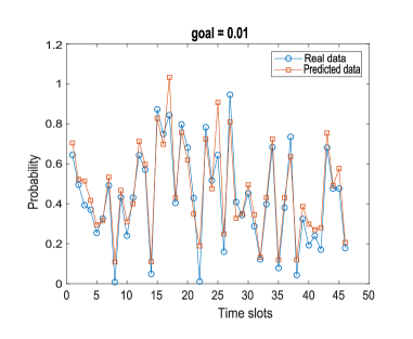
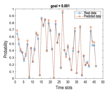
First, we evaluates the performance of the proposed LSTMs based task prediction algorithm. In our scenario, we assume that the user requests different tasks in different time slots. Meanwhile, the tasks have different popularity. We first generate the tasks’ popularity through a random walk model. Fig. 5 demonstrates the loss of the network with different learning rates. According to the figure, the proposed algorithm is capable of converging to a stable loss. The proposed LSTM converges faster with a higher learning rate. This is also justified in Remark 1. Fig. 6 compares real task popularity and predicted popularity. According to Fig. 6, we obtain better performance when we reduce the value of the goal.

V-B Simulation results of the proposed SAQ-learning algorithm for cache-aided NOMA MEC

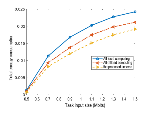
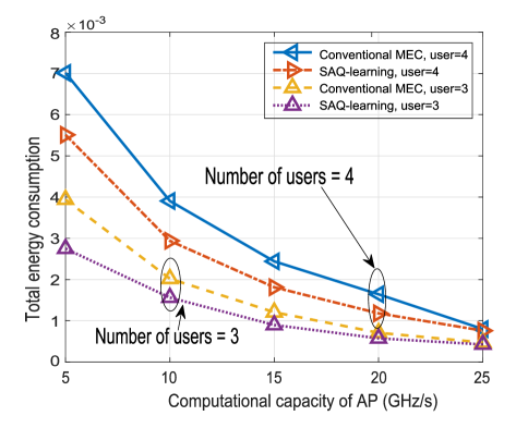
The simulation results of the proposed SAQL algorithm for cache-aided NOMA MEC is shown in Fig. 7 and Fig. 8. The total energy consumption vs. the task input size is shown in Fig. 7. A larger task input size requires more computing energy both for the mobile users and the MEC server. This is also justified in (6) and (9). In Fig. 7, the proposed cache-aided NOMA MEC outperforms both the all local computing and the all offload computing schemes. In Fig. 8, the proposed cache-aided NOMA MEC outperforms conventional MEC. The reason is that, in cache-aided MEC, the reusable task computing results are stored in the AP, which reduces the offloading and computing energy.

V-C Simulation results of the proposed BLA-MAQ-learning algorithm for cache-aided NOMA MEC

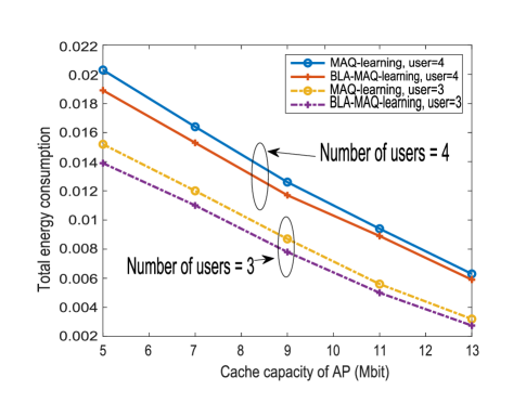
The simulation results of the proposed BLA-MAQ-learning algorithm for cache-aided NOMA MEC is shown in Fig. 9. As can be seen from Fig. 9, the total energy consumption decreases with the increase of caching capacity. This is because more computation results are stored in the AP, moreover, the offloading consumption and computing consumption of the same tasks required by other users are all reduced. As can be seen from Fig. 8, the total energy consumption decreases sharply with more computational capacity. Meanwhile, compared with Fig. 9, the total energy consumption decrease faster than increasing the cache capacity. This shows that increasing the computational capacity of the AP is a more efficient way of reducing total energy consumption compared with increasing the cache capacity of the AP.
Refer to caption
Figure 7: Total transmit energy consumption vs. task input size.
Refer to caption
Figure 8: Total energy consumption vs. the computation capacity of the AP.
Refer to caption
Figure 9: Total transmit energy consumption vs. cache capacity of the AP.
Refer to caption
Figure 10: The convergence of the proposed algorithm.

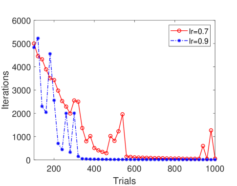
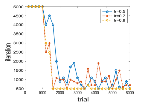
Finally, the convergence of the proposed algorithm is shown in Fig. 10. As can be seen from Fig. 10, the proposed algorithm converges faster with a higher learning rate. However, higher learning rate may cause overfit.

VI Conclusion

In this paper, a cache-aided NOMA MEC framework is proposed. In order to reduce the total energy consumption in cache-aided NOMA MEC networks, a joint long-term optimization problem is formulated, subject to caching and computing resources constraints in the AP. Three parameters are optimized in the formulated MINL problem. To make task offloading decisions of users and resource allocation for the AP, a SAQ-learning based resource allocation algorithm scheme was proposed. For the task offloading problem, a BAL-MAQ-learning algorithm is proposed, in which, the BLA based action selection scheme is adopted for every agent to obtain optimal action in every state. Simulation results demonstrated the performance of the proposed framework and algorithm. Our extensive simulation results demonstrated that increasing computation capacity of the AP was a more efficient method to reduce the total energy consumption compared with increasing caching capacity. One promising extension of this work is to consider more complicated joint learning algorithms for networks with multiple MEC servers, that require cooperation between the caching resource and computing resource. Moreover, incorporating the optimization of uploading power and computing allocation can further improve energy efficiency of multi-server networks, which is another promising future research direction.

Appendix A: Proof of Proposition 1

In Eq. (19), the partial derivative contains two parts: the first is the output 𝐨𝐭subscript𝐨𝐭{\bf{{o_{t}}}}, and the second part is the memory cell state 𝐂𝐭subscript𝐂𝐭{\bf{{C_{t}}}}. The detail is in Eq. (33). The partial derivatives of (𝐨𝐭)/(𝐰𝐂)subscript𝐨𝐭/subscript𝐰𝐂{{\partial\left({{{\bf{o}}_{\bf{t}}}}\right)}\mathord{\left/{\vphantom{{\partial\left({{{\bf{o}}_{\bf{t}}}}\right)}{\partial\left({{{\bf{w}}_{\bf{C}}}}\right)}}}\right.\kern-1.2pt}{\partial\left({{{\bf{w}}_{\bf{C}}}}\right)}} are given in Eq. (34). Based on Eq. (14), we can write a recursive equation as in Eq. (35). Combining Eq. (11), (12), (13), we obtain Eq. (36) (37) (38). Next, we can obtain Eq. (19). Finally, the proof is complete.

(𝐨𝐭tanh(𝐂𝐭))(𝐰𝐂)subscript𝐨𝐭subscript𝐂𝐭subscript𝐰𝐂\displaystyle\frac{{\partial\left({{{\bf{o}}_{\bf{t}}}\tanh\left({{{\bf{C}}_{\bf{t}}}}\right)}\right)}}{{\partial\left({{{\bf{w}}_{\bf{C}}}}\right)}} =(𝐨𝐭)(𝐰𝐂)tanh(𝐂𝐭)+𝐨𝐭(tanh(𝐂𝐭))(𝐰𝐂)absentsubscript𝐨𝐭subscript𝐰𝐂subscript𝐂𝐭subscript𝐨𝐭subscript𝐂𝐭subscript𝐰𝐂\displaystyle=\frac{{\partial\left({{{\bf{o}}_{\bf{t}}}}\right)}}{{\partial\left({{{\bf{w}}_{\bf{C}}}}\right)}}\tanh\left({{{\bf{C}}_{\bf{t}}}}\right)+{{\bf{o}}_{\bf{t}}}\frac{{\partial\left({\tanh\left({{{\bf{C}}_{\bf{t}}}}\right)}\right)}}{{\partial\left({{{\bf{w}}_{\bf{C}}}}\right)}} (33)
=(𝐨𝐭)(𝐰𝐂)tanh(𝐂𝐭)+𝐨𝐭(tanh(𝐂𝐭))(𝐂𝐭)(𝐂𝐭)(𝐰𝐂).absentsubscript𝐨𝐭subscript𝐰𝐂subscript𝐂𝐭subscript𝐨𝐭subscript𝐂𝐭subscript𝐂𝐭subscript𝐂𝐭subscript𝐰𝐂\displaystyle=\frac{{\partial\left({{{\bf{o}}_{\bf{t}}}}\right)}}{{\partial\left({{{\bf{w}}_{\bf{C}}}}\right)}}\tanh\left({{{\bf{C}}_{\bf{t}}}}\right)+{{\bf{o}}_{\bf{t}}}\frac{{\partial\left({\tanh\left({{{\bf{C}}_{\bf{t}}}}\right)}\right)}}{{\partial\left({{{\bf{C}}_{\bf{t}}}}\right)}}\frac{{\partial\left({{{\bf{C}}_{\bf{t}}}}\right)}}{{\partial\left({{{\bf{w}}_{\bf{C}}}}\right)}}.
(𝐨𝐭)(𝐰𝐂)subscript𝐨𝐭subscript𝐰𝐂\displaystyle{\bf\frac{{\partial\left({{o_{t}}}\right)}}{{\partial\left({{w_{C}}}\right)}}} =(σ(𝐖𝐨[𝐡𝐭𝟏,𝐱𝐭]+𝐛𝐨))(𝐰𝐂)absent𝜎subscript𝐖𝐨subscript𝐡𝐭1subscript𝐱𝐭subscript𝐛𝐨subscript𝐰𝐂\displaystyle={\bf\frac{{\partial\left({\sigma\left({{W_{o}}\left[{{h_{t-1}},{x_{t}}}\right]+{b_{o}}}\right)}\right)}}{{\partial\left({{w_{C}}}\right)}}} (34)
=(σ(𝐖𝐨[𝐨𝐭𝟏tanh(𝐂𝐭𝟏),𝐱𝐭]+𝐛𝐨))(𝐰𝐂)absent𝜎subscript𝐖𝐨subscript𝐨𝐭1subscript𝐂𝐭1subscript𝐱𝐭subscript𝐛𝐨subscript𝐰𝐂\displaystyle={\bf\frac{{\partial\left({\sigma\left({{W_{o}}\left[{{o_{t-1}}*\tanh\left({{C_{t-1}}}\right),{x_{t}}}\right]+{b_{o}}}\right)}\right)}}{{\partial\left({{w_{C}}}\right)}}}
=(σ)(𝐖𝐨[𝐡𝐭𝟏,𝐱𝐭]+𝐛𝐨)[𝐖𝐨(𝐨𝐭𝟏)(𝐰𝐂)tanh(𝐂𝐭𝟏)+𝐖𝐨𝐨𝐭𝟏(tanh(𝐂𝐭𝟏))(𝐰𝐂)].absent𝜎subscript𝐖𝐨subscript𝐡𝐭1subscript𝐱𝐭subscript𝐛𝐨delimited-[]subscript𝐖𝐨subscript𝐨𝐭1subscript𝐰𝐂subscript𝐂𝐭1subscript𝐖𝐨subscript𝐨𝐭1subscript𝐂𝐭1subscript𝐰𝐂\displaystyle={\bf\frac{{\partial\left(\sigma\right)}}{{\partial\left({{W_{o}}\left[{{h_{t-1}},{x_{t}}}\right]+{b_{o}}}\right)}}\left[{{W_{o}}\frac{{\partial\left({{o_{t-1}}}\right)}}{{\partial\left({{w_{C}}}\right)}}\tanh\left({{C_{t-1}}}\right)+{W_{o}}{o_{t-1}}\frac{{\partial\left({\tanh\left({{C_{t-1}}}\right)}\right)}}{{\partial\left({{w_{C}}}\right)}}}\right]}.
(𝐂𝐭)(𝐰𝐂)=𝐂𝐭𝟏(𝐟𝐭)(𝐰𝐂)+𝐟𝐭(𝐂𝐭𝟏)(𝐰𝐂)+𝐝𝐭(𝐢𝐭)(𝐰𝐂)+𝐢𝐭(𝐝𝐭)(𝐰𝐂).subscript𝐂𝐭subscript𝐰𝐂subscript𝐂𝐭1subscript𝐟𝐭subscript𝐰𝐂subscript𝐟𝐭subscript𝐂𝐭1subscript𝐰𝐂subscript𝐝𝐭subscript𝐢𝐭subscript𝐰𝐂subscript𝐢𝐭subscript𝐝𝐭subscript𝐰𝐂{\bf\frac{{\partial\left({{C_{t}}}\right)}}{{\partial\left({{w_{C}}}\right)}}\\ ={C_{t-1}}\frac{{\partial\left({{f_{t}}}\right)}}{{\partial\left({{w_{C}}}\right)}}+{f_{t}}\frac{{\partial\left({{C_{t-1}}}\right)}}{{\partial\left({{w_{C}}}\right)}}+{d_{t}}\frac{{\partial\left({{i_{t}}}\right)}}{{\partial\left({{w_{C}}}\right)}}+{i_{t}}\frac{{\partial\left({{d_{t}}}\right)}}{{\partial\left({{w_{C}}}\right)}}.} (35)
(𝐟𝐭)(𝐰𝐂)=(σ𝐟)(𝐖𝐟[𝐡𝐭𝟏,𝐱𝐭]+𝐛𝐟)[𝐖𝐟(𝐨𝐭𝟏)(𝐰𝐂)tanh(𝐂𝐭𝟏)+𝐖𝐟𝐨𝐭𝟏(tanh(𝐂𝐭𝟏))(𝐰𝐂)].subscript𝐟𝐭subscript𝐰𝐂subscript𝜎𝐟subscript𝐖𝐟subscript𝐡𝐭1subscript𝐱𝐭subscript𝐛𝐟delimited-[]subscript𝐖𝐟subscript𝐨𝐭1subscript𝐰𝐂subscript𝐂𝐭1subscript𝐖𝐟subscript𝐨𝐭1subscript𝐂𝐭1subscript𝐰𝐂\displaystyle{\bf\frac{{\partial\left({{f_{t}}}\right)}}{{\partial\left({{w_{C}}}\right)}}=\frac{{\partial\left({{\sigma_{f}}}\right)}}{{\partial\left({{W_{f}}\left[{{h_{t-1}},{x_{t}}}\right]+{b_{f}}}\right)}}\left[{{W_{f}}\frac{{\partial\left({{o_{t-1}}}\right)}}{{\partial\left({{w_{C}}}\right)}}\tanh\left({{C_{t-1}}}\right)+{W_{f}}{o_{t-1}}\frac{{\partial\left({\tanh\left({{C_{t-1}}}\right)}\right)}}{{\partial\left({{w_{C}}}\right)}}}\right].} (36)
(𝐢𝐭)(𝐰𝐂)=(σ𝐟)(𝐖𝐢[𝐡𝐭𝟏,𝐱𝐭]+𝐛𝐢)[𝐖𝐢(𝐨𝐭𝟏)(𝐰𝐂)tanh(𝐂𝐭𝟏)+𝐖𝐢𝐨𝐭𝟏(tanh(𝐂𝐭𝟏))(𝐰𝐂)].subscript𝐢𝐭subscript𝐰𝐂subscript𝜎𝐟subscript𝐖𝐢subscript𝐡𝐭1subscript𝐱𝐭subscript𝐛𝐢delimited-[]subscript𝐖𝐢subscript𝐨𝐭1subscript𝐰𝐂subscript𝐂𝐭1subscript𝐖𝐢subscript𝐨𝐭1subscript𝐂𝐭1subscript𝐰𝐂\displaystyle{\bf\frac{{\partial\left({{i_{t}}}\right)}}{{\partial\left({{w_{C}}}\right)}}=\frac{{\partial\left({{\sigma_{f}}}\right)}}{{\partial\left({{W_{i}}\left[{{h_{t-1}},{x_{t}}}\right]+{b_{i}}}\right)}}\left[{{W_{i}}\frac{{\partial\left({{o_{t-1}}}\right)}}{{\partial\left({{w_{C}}}\right)}}\tanh\left({{C_{t-1}}}\right)+{W_{i}}{o_{t-1}}\frac{{\partial\left({\tanh\left({{C_{t-1}}}\right)}\right)}}{{\partial\left({{w_{C}}}\right)}}}\right].} (37)
(𝐝𝐭)(𝐰𝐂)=(σ𝐟)(𝐖𝐝[𝐡𝐭𝟏,𝐱𝐭]+𝐛𝐝)[𝐖𝐝(𝐨𝐭𝟏)(𝐰𝐂)tanh(𝐂𝐭𝟏)+𝐖𝐝𝐨𝐭𝟏(tanh(𝐂𝐭𝟏))(𝐰𝐂)].subscript𝐝𝐭subscript𝐰𝐂subscript𝜎𝐟subscript𝐖𝐝subscript𝐡𝐭1subscript𝐱𝐭subscript𝐛𝐝delimited-[]subscript𝐖𝐝subscript𝐨𝐭1subscript𝐰𝐂subscript𝐂𝐭1subscript𝐖𝐝subscript𝐨𝐭1subscript𝐂𝐭1subscript𝐰𝐂\displaystyle{\bf\frac{{\partial\left({{d_{t}}}\right)}}{{\partial\left({{w_{C}}}\right)}}=\frac{{\partial\left({{\sigma_{f}}}\right)}}{{\partial\left({{W_{d}}\left[{{h_{t-1}},{x_{t}}}\right]+{b_{d}}}\right)}}\left[{{W_{d}}\frac{{\partial\left({{o_{t-1}}}\right)}}{{\partial\left({{w_{C}}}\right)}}\tanh\left({{C_{t-1}}}\right)+{W_{d}}{o_{t-1}}\frac{{\partial\left({\tanh\left({{C_{t-1}}}\right)}\right)}}{{\partial\left({{w_{C}}}\right)}}}\right].} (38)

Appendix B: Proof of Theorem 1

In each iteration, the computation task is either computed locally or is offloaded to the MEC server for computing. The probability that the agent chooses local computing at iteration n𝑛n is p1r2[α1n,β1n]superscriptsubscript𝑝1subscript𝑟2superscriptsubscript𝛼1𝑛superscriptsubscript𝛽1𝑛p_{1}^{{r_{2}}}\left[{\alpha_{1}^{n},\beta_{1}^{n}}\right], where (α1n,β1n)superscriptsubscript𝛼1𝑛superscriptsubscript𝛽1𝑛\left({\alpha_{1}^{n},\beta_{1}^{n}}\right) are the parameters of the Beta distribution associated with local computing. According to the characteristic of the Beta distribution, the probability of local computing (i.e., expected value) is 𝔼local=α1n/(α1n+β1n)subscript𝔼𝑙𝑜𝑐𝑎𝑙superscriptsubscript𝛼1𝑛/superscriptsubscript𝛼1𝑛superscriptsubscript𝛽1𝑛{{\mathbb{E}}_{local}}={{\alpha_{1}^{n}}\mathord{\left/{\vphantom{{\alpha_{1}^{n}}{\left({\alpha_{1}^{n}+\beta_{1}^{n}}\right)}}}\right.\kern-1.2pt}{\left({\alpha_{1}^{n}+\beta_{1}^{n}}\right)}}. In addition, the probability of offloaded computing is 1p1r2[α1n,β1n]1superscriptsubscript𝑝1subscript𝑟2superscriptsubscript𝛼1𝑛superscriptsubscript𝛽1𝑛1-p_{1}^{{r_{2}}}\left[{\alpha_{1}^{n},\beta_{1}^{n}}\right]. The feedback of local computing provides a reward with probability r1subscript𝑟1{r_{1}}, and a penalty with probability 1r11subscript𝑟11-{r_{1}}. Meanwhile, if offload computing is chosen by the agent, we have p1r2[α1n+1,β1n+1]=p1r2[α1n,β1n]superscriptsubscript𝑝1subscript𝑟2superscriptsubscript𝛼1𝑛1superscriptsubscript𝛽1𝑛1superscriptsubscript𝑝1subscript𝑟2superscriptsubscript𝛼1𝑛superscriptsubscript𝛽1𝑛p_{1}^{{r_{2}}}\left[{\alpha_{1}^{n+1},\beta_{1}^{n+1}}\right]=p_{1}^{{r_{2}}}\left[{\alpha_{1}^{n},\beta_{1}^{n}}\right], because r2subscript𝑟2{r_{2}} is given, and there is no feedback from local computing. Therefore we have:

𝔼{p1r2[α1n+1,β1n+1]|p1r2[α1n,β1n]}=(p1r2[α1n+1,β1n]r1+p1r2[α1n,β1n+1](1r1))=(p1r2[α1n,β1n]+p1r2[α1n,β1n](1p1r2[α1n,β1n])).𝔼conditional-setsuperscriptsubscript𝑝1subscript𝑟2superscriptsubscript𝛼1𝑛1superscriptsubscript𝛽1𝑛1superscriptsubscript𝑝1subscript𝑟2superscriptsubscript𝛼1𝑛superscriptsubscript𝛽1𝑛absentsuperscriptsubscript𝑝1subscript𝑟2superscriptsubscript𝛼1𝑛1superscriptsubscript𝛽1𝑛subscript𝑟1superscriptsubscript𝑝1subscript𝑟2superscriptsubscript𝛼1𝑛superscriptsubscript𝛽1𝑛11subscript𝑟1absentsuperscriptsubscript𝑝1subscript𝑟2superscriptsubscript𝛼1𝑛superscriptsubscript𝛽1𝑛superscriptsubscript𝑝1subscript𝑟2superscriptsubscript𝛼1𝑛superscriptsubscript𝛽1𝑛1superscriptsubscript𝑝1subscript𝑟2superscriptsubscript𝛼1𝑛superscriptsubscript𝛽1𝑛\begin{array}[]{l}{\mathbb{E}}\left\{{p_{1}^{{r_{2}}}\left[{\alpha_{1}^{n+1},\beta_{1}^{n+1}}\right]|p_{1}^{{r_{2}}}\left[{\alpha_{1}^{n},\beta_{1}^{n}}\right]}\right\}\\ =\left({p_{1}^{{r_{2}}}\left[{\alpha_{1}^{n}+1,\beta_{1}^{n}}\right]{r_{1}}+p_{1}^{{r_{2}}}\left[{\alpha_{1}^{n},\beta_{1}^{n}+1}\right]\left({1-{r_{1}}}\right)}\right)\\ =\left({p_{1}^{{r_{2}}}\left[{\alpha_{1}^{n},\beta_{1}^{n}}\right]+p_{1}^{{r_{2}}}\left[{\alpha_{1}^{n},\beta_{1}^{n}}\right]\left({1-p_{1}^{{r_{2}}}\left[{\alpha_{1}^{n},\beta_{1}^{n}}\right]}\right)}\right).\end{array} (39)

Then, by dividing the left and right side of the inequality, we can obtain Eq. (43).

E[p1r2(α1n+1,β1n+1)|p1r2(α1n,β1n)]>p1r2[α1n,β1n]p1r2(α1n+1,β1n)r1+p1r2(α1n,β1n+1)(1r1)+(1p1r2(α1n,β1n))>1p1r2(α1n+1,β1n)r1+p1r2(α1n,β1n+1)(1r1)>p1r2(α1n,β1n)𝐸delimited-[]conditionalsuperscriptsubscript𝑝1subscript𝑟2superscriptsubscript𝛼1𝑛1superscriptsubscript𝛽1𝑛1superscriptsubscript𝑝1subscript𝑟2superscriptsubscript𝛼1𝑛superscriptsubscript𝛽1𝑛superscriptsubscript𝑝1subscript𝑟2superscriptsubscript𝛼1𝑛superscriptsubscript𝛽1𝑛absentsuperscriptsubscript𝑝1subscript𝑟2superscriptsubscript𝛼1𝑛1superscriptsubscript𝛽1𝑛subscript𝑟1superscriptsubscript𝑝1subscript𝑟2superscriptsubscript𝛼1𝑛superscriptsubscript𝛽1𝑛11subscript𝑟11superscriptsubscript𝑝1subscript𝑟2superscriptsubscript𝛼1𝑛superscriptsubscript𝛽1𝑛1absentsuperscriptsubscript𝑝1subscript𝑟2superscriptsubscript𝛼1𝑛1superscriptsubscript𝛽1𝑛subscript𝑟1superscriptsubscript𝑝1subscript𝑟2superscriptsubscript𝛼1𝑛superscriptsubscript𝛽1𝑛11subscript𝑟1superscriptsubscript𝑝1subscript𝑟2superscriptsubscript𝛼1𝑛superscriptsubscript𝛽1𝑛\displaystyle\begin{array}[]{l}E\left[{p_{1}^{{r_{2}}}\left({\alpha_{1}^{n+1},\beta_{1}^{n+1}}\right)|p_{1}^{{r_{2}}}\left({\alpha_{1}^{n},\beta_{1}^{n}}\right)}\right]>p_{1}^{{r_{2}}}\left[{\alpha_{1}^{n},\beta_{1}^{n}}\right]\\ \Leftrightarrow p_{1}^{{r_{2}}}\left({\alpha_{1}^{n}+1,\beta_{1}^{n}}\right){r_{1}}+p_{1}^{{r_{2}}}\left({\alpha_{1}^{n},\beta_{1}^{n}+1}\right)\left({1-{r_{1}}}\right)+\left({1-p_{1}^{{r_{2}}}\left({\alpha_{1}^{n},\beta_{1}^{n}}\right)}\right)>1\\ \Leftrightarrow p_{1}^{{r_{2}}}\left({\alpha_{1}^{n}+1,\beta_{1}^{n}}\right){r_{1}}+p_{1}^{{r_{2}}}\left({\alpha_{1}^{n},\beta_{1}^{n}+1}\right)\left({1-{r_{1}}}\right)>p_{1}^{{r_{2}}}\left({\alpha_{1}^{n},\beta_{1}^{n}}\right)\end{array} (43)

In order to prove Theorem 1, we need to prove that the following is true:

𝔼{p1r2[α1n+1,β1n+1]|p1r2[α1n,β1n]}>p1r2[α1n,β1n]α1nα2n+β2n<r1.𝔼conditional-setsuperscriptsubscript𝑝1subscript𝑟2superscriptsubscript𝛼1𝑛1superscriptsubscript𝛽1𝑛1superscriptsubscript𝑝1subscript𝑟2superscriptsubscript𝛼1𝑛superscriptsubscript𝛽1𝑛superscriptsubscript𝑝1subscript𝑟2superscriptsubscript𝛼1𝑛superscriptsubscript𝛽1𝑛absentsuperscriptsubscript𝛼1𝑛superscriptsubscript𝛼2𝑛superscriptsubscript𝛽2𝑛subscript𝑟1\begin{array}[]{l}{\mathbb{E}}\left\{{p_{1}^{{r_{2}}}\left[{\alpha_{1}^{n+1},\beta_{1}^{n+1}}\right]|p_{1}^{{r_{2}}}\left[{\alpha_{1}^{n},\beta_{1}^{n}}\right]}\right\}>p_{1}^{{r_{2}}}\left[{\alpha_{1}^{n},\beta_{1}^{n}}\right]\\ \Leftrightarrow\frac{{\alpha_{1}^{n}}}{{\alpha_{2}^{n}+\beta_{2}^{n}}}<{r_{1}}.\end{array} (44)

According to the characteristics of the Beta distribution, the probability density function (PDF) of the beta distribution is

f(x;α,β)=xα1(1x)β101uα1(1u)β1𝑑u=Γ(α+β)Γ(α)Γ(β)xα1(1x)β1.𝑓𝑥𝛼𝛽superscript𝑥𝛼1superscript1𝑥𝛽1superscriptsubscript01superscript𝑢𝛼1superscript1𝑢𝛽1differential-d𝑢Γ𝛼𝛽Γ𝛼Γ𝛽superscript𝑥𝛼1superscript1𝑥𝛽1f\left({x;\alpha,\beta}\right)=\frac{{{x^{\alpha-1}}{{\left({1-x}\right)}^{\beta-1}}}}{{\int_{0}^{1}{{u^{\alpha-1}}{{\left({1-u}\right)}^{\beta-1}}du}}}=\frac{{\Gamma\left({\alpha+\beta}\right)}}{{\Gamma\left(\alpha\right)\Gamma\left(\beta\right)}}{x^{\alpha-1}}{\left({1-x}\right)^{\beta-1}}. (45)
p1r2[α1n+1,β1n]r1+p1r2[α1n,β1n+1](1r1)>p1r2[α1n,β1n](1F(r2;α1n+1,β1n))r1+(1F(r2;α1n,β1n+1))(1r1)>1F(r2;α1n,β1n)F(r2;α1n,β1n)r1F(r2;α1n+1,β1n)(1r1)F(r2;α1n,β1n+1)>0F(r2;α1n,β1n)r1(F(r2;α1n,β1n)+(α1n+β1n1)!α1n!(β1n1)!(1x)β1nxα1n)(1r1)(F(r2;α1n,β1n)+(α1n+β1n1)!β1n!(α1n1)!(1x)β1nxα1n)α1nα1n+β1n<r1.superscriptsubscript𝑝1subscript𝑟2superscriptsubscript𝛼1𝑛1superscriptsubscript𝛽1𝑛subscript𝑟1superscriptsubscript𝑝1subscript𝑟2superscriptsubscript𝛼1𝑛superscriptsubscript𝛽1𝑛11subscript𝑟1superscriptsubscript𝑝1subscript𝑟2superscriptsubscript𝛼1𝑛superscriptsubscript𝛽1𝑛absent1𝐹subscript𝑟2superscriptsubscript𝛼1𝑛1superscriptsubscript𝛽1𝑛subscript𝑟11𝐹subscript𝑟2superscriptsubscript𝛼1𝑛superscriptsubscript𝛽1𝑛11subscript𝑟11𝐹subscript𝑟2superscriptsubscript𝛼1𝑛superscriptsubscript𝛽1𝑛absent𝐹subscript𝑟2superscriptsubscript𝛼1𝑛superscriptsubscript𝛽1𝑛subscript𝑟1𝐹subscript𝑟2superscriptsubscript𝛼1𝑛1superscriptsubscript𝛽1𝑛1subscript𝑟1𝐹subscript𝑟2superscriptsubscript𝛼1𝑛superscriptsubscript𝛽1𝑛10absent𝐹subscript𝑟2superscriptsubscript𝛼1𝑛superscriptsubscript𝛽1𝑛subscript𝑟1𝐹subscript𝑟2superscriptsubscript𝛼1𝑛superscriptsubscript𝛽1𝑛superscriptsubscript𝛼1𝑛superscriptsubscript𝛽1𝑛1superscriptsubscript𝛼1𝑛superscriptsubscript𝛽1𝑛1superscript1𝑥superscriptsubscript𝛽1𝑛superscript𝑥superscriptsubscript𝛼1𝑛1subscript𝑟1𝐹subscript𝑟2superscriptsubscript𝛼1𝑛superscriptsubscript𝛽1𝑛superscriptsubscript𝛼1𝑛superscriptsubscript𝛽1𝑛1superscriptsubscript𝛽1𝑛superscriptsubscript𝛼1𝑛1superscript1𝑥superscriptsubscript𝛽1𝑛superscript𝑥superscriptsubscript𝛼1𝑛absentsuperscriptsubscript𝛼1𝑛superscriptsubscript𝛼1𝑛superscriptsubscript𝛽1𝑛subscript𝑟1\displaystyle\begin{array}[]{l}p_{1}^{{r_{2}}}\left[{\alpha_{1}^{n}+1,\beta_{1}^{n}}\right]{r_{1}}+p_{1}^{{r_{2}}}\left[{\alpha_{1}^{n},\beta_{1}^{n}+1}\right]\left({1-{r_{1}}}\right)>p_{1}^{{r_{2}}}\left[{\alpha_{1}^{n},\beta_{1}^{n}}\right]\\ \Leftrightarrow\left({1-F\left({{r_{2}};\alpha_{1}^{n}+1,\beta_{1}^{n}}\right)}\right){r_{1}}+\left({1-F\left({{r_{2}};\alpha_{1}^{n},\beta_{1}^{n}+1}\right)}\right)\left({1-{r_{1}}}\right)>1-F\left({{r_{2}};\alpha_{1}^{n},\beta_{1}^{n}}\right)\\ \Leftrightarrow F\left({{r_{2}};\alpha_{1}^{n},\beta_{1}^{n}}\right)-{r_{1}}F\left({{r_{2}};\alpha_{1}^{n}+1,\beta_{1}^{n}}\right)-\left({1-{r_{1}}}\right)F\left({{r_{2}};\alpha_{1}^{n},\beta_{1}^{n}+1}\right)>0\\ \Leftrightarrow F\left({{r_{2}};\alpha_{1}^{n},\beta_{1}^{n}}\right)-{r_{1}}\left({F\left({{r_{2}};\alpha_{1}^{n},\beta_{1}^{n}}\right)+\frac{{\left({\alpha_{1}^{n}+\beta_{1}^{n}-1}\right)!}}{{\alpha_{1}^{n}!\left({\beta_{1}^{n}-1}\right)!}}{{\left({1-x}\right)}^{\beta_{1}^{n}}}{x^{\alpha_{1}^{n}}}}\right)-...\\ \left({1-{r_{1}}}\right)\left({F\left({{r_{2}};\alpha_{1}^{n},\beta_{1}^{n}}\right)+\frac{{\left({\alpha_{1}^{n}+\beta_{1}^{n}-1}\right)!}}{{\beta_{1}^{n}!\left({\alpha_{1}^{n}-1}\right)!}}{{\left({1-x}\right)}^{\beta_{1}^{n}}}{x^{\alpha_{1}^{n}}}}\right)\\ \Leftrightarrow\frac{{\alpha_{1}^{n}}}{{\alpha_{1}^{n}+\beta_{1}^{n}}}<{r_{1}}.\end{array} (52)

The expected value (mean) of a Beta distribution random variable X𝑋X is

𝔼(X)=o1xf(x;α,β)𝑑x=o1xΓ(α+β)Γ(α)Γ(β)xα1(1x)β1𝑑x.𝔼𝑋superscriptsubscript𝑜1𝑥𝑓𝑥𝛼𝛽differential-d𝑥superscriptsubscript𝑜1𝑥Γ𝛼𝛽Γ𝛼Γ𝛽superscript𝑥𝛼1superscript1𝑥𝛽1differential-d𝑥{\mathbb{E}}\left(X\right)=\int_{o}^{1}{xf\left({x;\alpha,\beta}\right)dx}=\int_{o}^{1}{x\frac{{\Gamma\left({\alpha+\beta}\right)}}{{\Gamma\left(\alpha\right)\Gamma\left(\beta\right)}}{x^{\alpha-1}}{{\left({1-x}\right)}^{\beta-1}}dx}. (53)

According to the fact that:

o1Γ(α+β+1)Γ(α+1)Γ(β)tα1(1t)β1𝑑t=1.superscriptsubscript𝑜1Γ𝛼𝛽1Γ𝛼1Γ𝛽superscript𝑡𝛼1superscript1𝑡𝛽1differential-d𝑡1\int_{o}^{1}{\frac{{\Gamma\left({\alpha+\beta+1}\right)}}{{\Gamma\left({\alpha+1}\right)\Gamma\left(\beta\right)}}{t^{\alpha-1}}{{\left({1-t}\right)}^{\beta-1}}dt}=1. (54)
F(x;α+1,β)=F(x;α,β)+(α+β1)!α!(β1)!(1x)βxα,𝐹𝑥𝛼1𝛽𝐹𝑥𝛼𝛽𝛼𝛽1𝛼𝛽1superscript1𝑥𝛽superscript𝑥𝛼F\left({x;\alpha+1,\beta}\right)=F\left({x;\alpha,\beta}\right)+\frac{{\left({\alpha+\beta-1}\right)!}}{{\alpha!\left({\beta-1}\right)!}}{\left({1-x}\right)^{\beta}}{x^{\alpha}}, (55)
F(x;α,β+1)=F(x;α,β)+(α+β1)!β!(α1)!(1x)βxα.𝐹𝑥𝛼𝛽1𝐹𝑥𝛼𝛽𝛼𝛽1𝛽𝛼1superscript1𝑥𝛽superscript𝑥𝛼F\left({x;\alpha,\beta+1}\right)=F\left({x;\alpha,\beta}\right)+\frac{{\left({\alpha+\beta-1}\right)!}}{{\beta!\left({\alpha-1}\right)!}}{\left({1-x}\right)^{\beta}}{x^{\alpha}}. (56)

The cumulative distribution function is given by:

F(x;α,β)=k=αα+β+1(α+β+1)!k!(α+β1k)!xk(1x)α+β1k.𝐹𝑥𝛼𝛽superscriptsubscript𝑘𝛼𝛼𝛽1𝛼𝛽1𝑘𝛼𝛽1𝑘superscript𝑥𝑘superscript1𝑥𝛼𝛽1𝑘F\left({x;\alpha,\beta}\right)=\sum\limits_{k=\alpha}^{\alpha+\beta+1}{\frac{{\left({\alpha+\beta+1}\right)!}}{{k!\left({\alpha+\beta-1-k}\right)!}}{x^{k}}{{\left({1-x}\right)}^{\alpha+\beta-1-k}}}. (57)

Then, the probability p1(α1n,β1n|r2)subscript𝑝1superscriptsubscript𝛼1𝑛conditionalsuperscriptsubscript𝛽1𝑛subscript𝑟2{p_{1}}\left({\alpha_{1}^{n},\beta_{1}^{n}|{r_{2}}}\right) is given by

p1r2(α1n,β1n)=P(X1N>r2|α1n,β1n)=1F(r2;α1n,β1n).superscriptsubscript𝑝1subscript𝑟2superscriptsubscript𝛼1𝑛superscriptsubscript𝛽1𝑛𝑃superscriptsubscript𝑋1𝑁conditionalsubscript𝑟2superscriptsubscript𝛼1𝑛superscriptsubscript𝛽1𝑛1𝐹subscript𝑟2superscriptsubscript𝛼1𝑛superscriptsubscript𝛽1𝑛p_{1}^{{r_{2}}}\left({\alpha_{1}^{n},\beta_{1}^{n}}\right)=P\left({X_{1}^{N}>{r_{2}}|\alpha_{1}^{n},\beta_{1}^{n}}\right)=1-F\left({{r_{2}};\alpha_{1}^{n},\beta_{1}^{n}}\right). (58)

Therefore, substituting Eq. (58) in Eq. (44), we can get Eq. (52). Therefore, Eq. (44) is correct. The BLA based action selection scheme is capable of self-correcting to the local computing under the condition that the probability of choosing offload computing is higher than that of local computing.

Appendix C: Proof of Theorem 2

In order to prove Theorem 2, first we need to make an assumption, which is that there is only one optimal action, i.e., P(r1=r2)=0𝑃subscript𝑟1subscript𝑟20P\left({{r_{1}}={r_{2}}}\right)=0. If the probabilities of the two actions are the same, according to Theorem 1, the probability of selecting the optimal action will not increase given the worst situation (i.e., the probability of non-optimal action is higher than that of optimal action). In other words, the self-correcting feature of BLA vanishes.

Since all the quantities involved in Eq. (31) are positive, we obtain α2n>0superscriptsubscript𝛼2𝑛0\alpha_{2}^{n}>0. According to Theorem 1, the expected value 𝔼(Xi)=αinβin+αin𝔼subscript𝑋𝑖superscriptsubscript𝛼𝑖𝑛superscriptsubscript𝛽𝑖𝑛superscriptsubscript𝛼𝑖𝑛{\mathbb{E}}\left({{X_{i}}}\right)=\frac{{\alpha_{i}^{n}}}{{\beta_{i}^{n}+\alpha_{i}^{n}}} approaches risubscript𝑟𝑖r_{i} with the increase of time, i.e.:

𝔼(X1)=α1nβ1n+α1n=r1,𝔼subscript𝑋1superscriptsubscript𝛼1𝑛superscriptsubscript𝛽1𝑛superscriptsubscript𝛼1𝑛subscript𝑟1{\mathbb{E}}\left({{X_{1}}}\right)=\frac{{\alpha_{1}^{n}}}{{\beta_{1}^{n}+\alpha_{1}^{n}}}={r_{1}}, (59)
𝔼(X2)=α2nβ2n+α2n=r2.𝔼subscript𝑋2superscriptsubscript𝛼2𝑛superscriptsubscript𝛽2𝑛superscriptsubscript𝛼2𝑛subscript𝑟2{\mathbb{E}}\left({{X_{2}}}\right)=\frac{{\alpha_{2}^{n}}}{{\beta_{2}^{n}+\alpha_{2}^{n}}}={r_{2}}. (60)

Combining Eq. (62) and Eq. (60), we get

β1n=(1r1)α1nr1.superscriptsubscript𝛽1𝑛1subscript𝑟1superscriptsubscript𝛼1𝑛subscript𝑟1\beta_{1}^{n}=\frac{{\left({1-{r_{1}}}\right)\alpha_{1}^{n}}}{{{r_{1}}}}. (61)

According to [44], the probability of chosen local computing is given by

p1sBLAn=(β1n)!(α2n)!(β1n+α2n)!=((1r1)α1nr1)!(α2n)!((1r1)α1nr1+α2n)!=1.superscriptsubscript𝑝1superscriptsubscript𝑠𝐵𝐿𝐴𝑛superscriptsubscript𝛽1𝑛superscriptsubscript𝛼2𝑛superscriptsubscript𝛽1𝑛superscriptsubscript𝛼2𝑛1subscript𝑟1superscriptsubscript𝛼1𝑛subscript𝑟1superscriptsubscript𝛼2𝑛1subscript𝑟1superscriptsubscript𝛼1𝑛subscript𝑟1superscriptsubscript𝛼2𝑛1\displaystyle p_{1}^{s_{BLA}^{n}}{\rm{}}=\frac{{\left({\beta_{1}^{n}}\right)!\left({\alpha_{2}^{n}}\right)!}}{{\left({\beta_{1}^{n}+\alpha_{2}^{n}}\right)!}}=\frac{{\left({\frac{{\left({1-{r_{1}}}\right)\alpha_{1}^{n}}}{{{r_{1}}}}}\right)!\left({\alpha_{2}^{n}}\right)!}}{{\left({\frac{{\left({1-{r_{1}}}\right)\alpha_{1}^{n}}}{{{r_{1}}}}+\alpha_{2}^{n}}\right)!}}=1. (62)

The proof is complete.

References

  • [1] Z. Yang, Y. Liu, Y. Chen, and G. Tyson, “Deep reinforcement learning in cache-aided MEC networks,” in IEEE Proc. of International Commun. Conf. (ICC), Shanghai, China, May. 2019.
  • [2] M. Chen, Y. Hao, L. Hu, M. S. Hossain, and A. Ghoneim, “Edge-cocaco: Toward joint optimization of computation, caching, and communication on edge cloud,” IEEE Wireless Commun., vol. 25, no. 3, pp. 21–27, Jun. 2018.
  • [3] M. Liu, F. R. Yu, Y. Teng, V. C. M. Leung, and M. Song, “Distributed resource allocation in blockchain-based video streaming systems with mobile edge computing,” IEEE Trans. Wireless Commun., vol. 18, no. 1, pp. 695–708, Jan. 2019.
  • [4] Y. Mao, C. You, J. Zhang, K. Huang, and K. B. Letaief, “A survey on mobile edge computing: The communication perspective,” IEEE Commun. Surv. Tut., vol. 19, no. 4, pp. 2322–2358, four quarter 2017.
  • [5] Z. Qin, X. Yue, Y. Liu, Z. Ding, and A. Nallanathan, “User association and resource allocation in unified noma enabled heterogeneous ultra dense networks,” IEEE Commun. Mag., vol. 56, no. 6, pp. 86–92, Jun. 2018.
  • [6] Y. Liu, Z. Qin, M. Elkashlan, Z. Ding, A. Nallanathan, and L. Hanzo, “Nonorthogonal multiple access for 5G and beyond,” Proc. IEEE, vol. 105, no. 12, pp. 2347–2381, Dec. 2017.
  • [7] Z. Ding, Y. Liu, J. Choi, Q. Sun, M. Elkashlan, C. I, and H. V. Poor, “Application of non-orthogonal multiple access in LTE and 5G networks,” IEEE Commun. Mag., vol. 55, no. 2, pp. 185–191, Feb. 2017.
  • [8] L. Xiang, D. W. K. Ng, X. Ge, Z. Ding, V. W. S. Wong, and R. Schober, “Cache-aided non-orthogonal multiple access: The two-user case,” IEEE J. Sel. Topic Signal Processing., pp. 1–1, 2019.
  • [9] Y. Cui, W. He, C. Ni, C. Guo, and Z. Liu, “Energy-efficient resource allocation for cache-assisted mobile edge computing,” in IEEE Proc. of Loc. Com. Netw. (LCN), Oct. 2017, pp. 640–648.
  • [10] Y. Mao, J. Zhang, and K. B. Letaief, “Dynamic computation offloading for mobile-edge computing with energy harvesting devices,” IEEE J. Sel. Areas Commun., vol. 34, no. 12, pp. 3590–3605, Dec. 2016.
  • [11] C. You, K. Huang, H. Chae, and B. H. Kim, “Energy-efficient resource allocation for mobile-edge computation offloading,” IEEE Trans. Wireless Commun., vol. 16, no. 3, pp. 1397–1411, Mar. 2017.
  • [12] X. Chen, H. Zhang, C. Wu, S. Mao, Y. Ji, and M. Bennis, “Optimized computation offloading performance in virtual edge computing systems via deep reinforcement learning,” ArXiv, May 2018. [Online]. Available: http://arxiv.org/abs/1805.06146
  • [13] Z. Ding, P. Fan, and H. V. Poor, “Impact of non-orthogonal multiple access on the offloading of mobile edge computing,” IEEE Trans. Commun., vol. 67, no. 1, pp. 375–390, Jan. 2019.
  • [14] F. Wang, J. Xu, and Z. Ding, “Multi-antenna NOMA for computation offloading in multiuser mobile edge computing systems,” IEEE Trans. Commun., vol. 67, no. 3, pp. 2450–2463, Mar. 2019.
  • [15] A. Kiani and N. Ansari, “Edge computing aware NOMA for 5G networks,” IEEE Int. of Things, vol. 5, no. 2, pp. 1299–1306, Apr. 2018.
  • [16] Y. Pan, M. Chen, Z. Yang, N. Huang, and M. Shikh-Bahaei, “Energy-efficient NOMA-based mobile edge computing offloading,” IEEE Commun. Lett., vol. 23, no. 2, pp. 310–313, Feb. 2019.
  • [17] Z. Ding, D. W. K. Ng, R. Schober, and H. V. Poor, “Delay minimization for NOMA-MEC offloading,” IEEE Signal Process. Lett., vol. 25, no. 12, pp. 1875–1879, Dec. 2018.
  • [18] Z. Song, Y. Liu, and X. Sun, “Joint radio and computational resource allocation for NOMA-based mobile edge computing in heterogeneous networks,” IEEE Commun. Lett., vol. 22, no. 12, pp. 2559–2562, Dec. 2018.
  • [19] M. Vaezi, G. Amarasuriya, Y. Liu, A. Arafa, and Z. D. Fang Fang, “Interplay between NOMA and other emerging technologies: A survey,” ArXiv, 2019. [Online]. Available: https://arxiv.org/abs/1903.10489
  • [20] Z. Ding, P. Fan, G. K. Karagiannidis, R. Schober, and H. V. Poor, “NOMA assisted wireless caching: Strategies and performance analysis,” IEEE Trans. Commun., vol. 66, no. 10, pp. 4854–4876, Oct. 2018.
  • [21] Z. Zhao, M. Xu, W. Xie, Z. Ding, and G. K. Karagiannidis, “Coverage performance of NOMA in wireless caching networks,” IEEE Commun. Lett., vol. 22, no. 7, pp. 1458–1461, Jul. 2018.
  • [22] L. Xiang, D. W. K. Ng, X. Ge, and Z. Ding, “Cache-aided non-orthogonal multiple access,” ArXiv, 2018. [Online]. Available: https://arxiv.org/abs/1712.09557
  • [23] J. A. Oviedo and H. R. Sadjadpour, “Leveraging edge caching in NOMA systems with QoS requirements,” ArXiv, 2019. [Online]. Available: https://arxiv.org/abs/1801.07430
  • [24] Y. Fu, Y. Liu, H. Wang, Z. Shi, and Y. Liu, “Mode selection between index coding and superposition coding in cache-based NOMA networks,” IEEE Commun. Lett., vol. 23, no. 3, pp. 478–481, Mar. 2019.
  • [25] L. Xiao, X. Wan, C. Dai, X. Du, X. Chen, and M. Guizani, “Security in mobile edge caching with reinforcement learning,” IEEE Wireless Commun., vol. 25, no. 3, pp. 116–122, Jun. 2018.
  • [26] Y. Zhou, F. R. Yu, J. Chen, and Y. Kuo, “Communications, caching, and computing for next generation HetNets,” IEEE Wireless Commun., vol. 25, no. 4, pp. 104–111, Aug. 2018.
  • [27] Narendra and Fukunaga, “A branch and bound algorithm for feature subset selection,” IEEE Trans. Comput., vol. C-26, no. 9, pp. 917–922, Sep. 1977.
  • [28] D. P. Bertsekas, Dynamic programming and optimal control.   Athena scientific Belmont, MA, 2005, vol. 1, no. 3.
  • [29] Z. Qin, H. Ye, G. Y. Li, and B. F. Juang, “Deep learning in physical layer communications,” IEEE Wireless Commun., vol. 26, no. 2, pp. 93–99, Apr. 2019.
  • [30] A. Bayati, K. Khoa Nguyen, and M. Cheriet, “Multiple-step-ahead traffic prediction in high-speed networks,” IEEE Commun. Lett., vol. 22, no. 12, pp. 2447–2450, Dec. 2018.
  • [31] K. Pichotta and R. J. Mooney, “Learning statistical scripts with LSTM recurrent neural networks,” The Thirtieth AAAI Conference on Artificial Intelligence (AAAI-16), 2016.
  • [32] Y. Wang, M. Long, J. Wang, Z. Gao, and P. S. Yu, “Predrnn: Recurrent neural networks for predictive learning using spatiotemporal LSTMs,” Advances in Neural Information Processing Systems 30 (NIPS-17), 2017.
  • [33] B. Du, C. Wu, and Z. Huang, “Learning resource allocation and pricing for cloud profit maximization,” The Thirty-Third AAAI Conference on Artificial Intelligence (AAAI-19), 2019.
  • [34] S. Ghoorchian and S. Maghsudi, “Multi-armed bandit for energy-efficient and delay-sensitive edge computing in dynamic networks with uncertainty,” ArXiv, 2019. [Online]. Available: https://arxiv.org/abs/1904.06258
  • [35] A. Asheralieva, “Bayesian reinforcement learning-based coalition formation for distributed resource sharing by device-to-device users in heterogeneous cellular networks,” IEEE Trans. Wireless Commun., vol. 16, no. 8, pp. 5016–5032, Aug. 2017.
  • [36] Z. Yang, Y. Liu, Y. Chen, and L. Jiao, “Learning automata based Q-learning for content placement in cooperative caching,” ArXiv, 2019. [Online]. Available: https://arxiv.org/abs/1903.06235
  • [37] F. Wang, J. Xu, X. Wang, and S. Cui, “Joint offloading and computing optimization in wireless powered mobile-edge computing systems,” IEEE Trans. Wireless Commun., vol. 17, no. 3, pp. 1784–1797, Mar. 2018.
  • [38] C. You, K. Huang, and H. Chae, “Energy efficient mobile cloud computing powered by wireless energy transfer,” IEEE J. Sel. Areas Commun., vol. 34, no. 5, pp. 1757–1771, May 2016.
  • [39] S. Hochreiter and J. Schmidhuber, “Long short-term memory,” Neural Comput., vol. 9, no. 8, pp. 1735–1780, Nov. 1997.
  • [40] R. J. Williams and D. Zipser, “A learning algorithm for continually running fully recurrent neural networks,” Neural Comput., vol. 1, no. 2, pp. 270–280, Jun. 1989.
  • [41] R. S. Sutton and A. G. Barto, Reinforcement Learning: An Introduction.   Cambridge, MA, USA: MIT Press, 2016.
  • [42] O. Granmo, “A bayesian learning automaton for solving two-armed bernoulli bandit problems,” in International Conference on Machine Learning and Applications, Dec. 2008, pp. 23–30.
  • [43] M. Chen, W. Saad, C. Yin, and M. Debbah, “Echo state networks for proactive caching in cloud-based radio access networks with mobile users,” IEEE Trans. Wireless Commun., vol. 16, no. 6, pp. 3520–3535, Jun. 2017.
  • [44] O.-C. Granmo, “Solving two-armed bernoulli bandit problems using a bayesian learning automaton,” International Journal of Intelligent Computing and Cybernetics, vol. 3, no. 2, pp. 207–234, 2010.