Computationally Efficient Distributed Multi-sensor Fusion with Multi-Bernoulli Filter

Wei Yi, Suqi Li, Bailu Wang, Reza Hoseinnezhad and Lingjiang Kong W. Yi, S. Li, B. Wang and L. Kong are with the School of Information and Communication Engineering, the University of Electronic Science and Technology of China. (Suqi Li is the corresponding author, Email:qi_qi_zhu1210@163.com) R. Hoseinnezhad is with the School of Engineering, RMIT University, Victoria 3083, Australia.
Abstract

This paper proposes a computationally efficient algorithm for distributed fusion in a sensor network in which multi-Bernoulli (MB) filters are locally running in every sensor node for multi-target tracking. The generalized Covariance Intersection (GCI) fusion rule is employed to fuse multiple MB random finite set densities. The fused density comprises a set of fusion hypotheses that grow exponentially with the number of Bernoulli components. Thus, GCI fusion with MB filters can become computationally intractable in practical applications that involve tracking of even a moderate number of objects. In order to accelerate the multi-sensor fusion procedure, we derive a theoretically sound approximation to the fused density. The number of fusion hypotheses in the resulting density is significantly smaller than the original fused density. It also has a parallelizable structure that allows multiple clusters of Bernoulli components to be fused independently. By carefully clustering Bernoulli components into isolated clusters using the GCI divergence as the distance metric, we propose an alternative to build exactly the approximated density without exhaustively computing all the fusion hypotheses. The combination of the proposed approximation technique and the fast clustering algorithm can enable a novel and fast GCI-MB fusion implementation. Our analysis shows that the proposed fusion method can dramatically reduce the computational and memory requirements with small bounded L1subscript𝐿1L_{1}-error. The Gaussian mixture implementation of the proposed method is also presented. In various numerical experiments, including a challenging scenario with up to forty objects, the efficacy of the proposed fusion method is demonstrated.

I Introduction

Distributed Multi-sensor Multi-object Tracking (DMMT) technology is recently advocated in the information fusion community, since it generally benefits from lower communication costs and immunity to single-node fault, compared with optimal centralized fusion solutions. In practice, the correlations between the posterior densities from different sensors are usually unknown, and this makes it very challenging to devise DMMT solutions. The optimal solution to this problem has been proposed by Chong et al. [1], but the heavy computational burden of extracting the common information can rule out this solution in many applications. A suboptimal solution with demonstrated tractability has been formulated based on the Generalized Covariance Intersection (GCI) method proposed by Mahler [2]. Essentially, GCI is the generalization of Covariance Intersection (CI) [3]. Compared to the CI fusion rule, which mainly utilizes the first and second order statistical characteristics of the single-object densities, the GCI fusion rule is capable to fuse multiple full multi-object densities with unknown correlations among sensor nodes, while intrinsically avoiding the double counting of common information [4]. The GCI fused multi-object density is also named as Exponential Mixture Density (EMD) [5, 6] or Kullback-Leibler Average (KLA) [7].

Clark et al. [8] derived tractable implementations of the GCI fusion rule for especial cases where the multi-object distributions are Poisson, independent identically distributed (i.i.d.) clusters and Bernoulli distributions. Utilizing these formulations, the GCI fusion method can be implemented for distributed fusion in sensor networks where the Probability Hypothesis Density (PHD)/Cardinalized PHD (CPHD) filter or the Bernoulli filter are running locally in every sensor node. Battistelli et al. [7] and Guldogan [9] proposed the Gaussian Mixture (GM) implementation of distributed fusion with CPHD filter and Bernoulli filter, respectively. Furthermore, a consensus approach to distributed multi-object tracking was first introduced in [7], with which the GCI fusion can be implemented in a fully distributed manner. The Sequential Monte Carlo (SMC) implementation of the GCI fusion with CPHD filter was proposed by Uney et al. [5].

Compared with PHD [10, 11] and CPHD [12, 13, 14, 15] filters, the Multi-Bernoulli (MB) filter [15, 16] can be more efficient and accurate in problems that require object individual existence probabilities. The performance of the MB filters has been well demonstrated in a wide range of practical monitoring problems such as radar tracking [17], video and audio tracking [16, 18], sensor control [19, 20], and acoustic sensor tracking [21]. In addition, a number of novel extensions of the MB recursion have also been investigated. Examples include the multiple model multi-Bernoulli filter proposed to cope with maneuvering objects [22], a robust multi-Bernoulli filter that can accommodate an unknown non-homogeneous clutter and detection profile [23], a joint multi-object estimator for multi-Bernoulli models [24], and a few enhanced multi-Bernoulli filters [25, 26].

The generalization of MB filters to the DMMT problem was firstly investigated in [27], where a distributed fusion algorithm based on GCI fusion rule (called GCI-MB in this paper) is proposed. While the enhanced performance of the GCI-MB fusion has been demonstrated [27], its major drawback is the heavy computational cost that increases exponentially with the number of objects in the surveillance area. For the DMMT over a sensor network, it is of paramount importance to reduce the local (in-node) computational expenses as much as possible, since in the typical distributed sensor networks, each node usually has limited processing power and energy resources.

In this paper, the computations involved in GCI-MB fusion are investigated, showing that the major contributor to the heavy computational burden is the exhaustive calculation of the weights and fused single-object densities of the GCI-MB fusion hypotheses, noting that the number of hypotheses increases super-exponentially with the number of objects. This observation provides the insight that leads to a novel computationally efficient and naturally parallelizable implementation of the GCI-MB fusion.

The major contributions are summarized as follows:

  1. 1.

    Devising a principled approximation to the fused density: By discarding all the insignificant GCI-MB fusion hypotheses with negligible weights, then normalizing the rest of hypotheses, we obtain a principled approximation to the original fused density. This approximation not only consists of significantly smaller number of fusion hypotheses but also enjoys an appealing structure: it can be factorized into several mutually independent and smaller size multi-object densities that lead to a principled independence approximation. Each of these factorized densities are shown to be equally returned by the GCI-MB fusion performed with a partial cluster of entire Bernoulli components. We also quantify the approximation error by deriving the L1subscript𝐿1L_{1}-error [28] between the original density and the approximated one, and show that it is reasonably small, and indeed, negligible for many practical applications.

  2. 2.

    Fast clustering of the Bernoulli components: The main challenge in obtaining the approximation is to truncate all the insignificant GCI-MB fusion hypotheses without computing them all in an exhaustive manner. To this end, by carefully clustering the Bernoulli components into isolated clusters according to a distance metric, i.e., GCI divergence, and then discarding the hypotheses of the association pairs of Bernoulli components from different isolated clusters among sensors, one can build exactly the independence approximation without exhaustively computing all the terms. By modeling the underline data structure of Bernoulli components among all sensors as a undirected graph, the clustering problem is tantamount to seeking connected components of a undirected graph dynamically, and can be solved by the disjoint-set data structure based fast solver with a computational cost that is only polynomial in the number of Bernoulli components.

  3. 3.

    Computationally efficient GCI-MB fusion: The combination of the independence approximation and the fast clustering algorithm can enable a computationally efficient fusion algorithm. The fast clustering algorithm is employed at an early stage to obtain the approximated density. Then by utilizing the structure of the approximated density, GCI fusion is performed within each smaller clusters of Bernoulli components independently and in a parallelized manner, namely, via performing fusion between each pair of the factorized multi-object densities among sensors. The GM implementation of the proposed fast GCI-MB fusion is also presented.

In numerical results, the efficiency and accuracy of the proposed fast GCI-MB fusion algorithm with GM implementation is tested in a challenging scenario with up to forty objects. Preliminary results have been published in the conference paper [29]. This paper presents a more complete theoretical and numerical study.

The rest of the paper is organized as follows. Background material and notation are introduced in Section II. The GCI-MB fusion is briefly reviewed and its computational intractability is discussed in Section III. Section IV devotes to the development of the proposed distributed fusion algorithm with MB filter based on the independence approximation and the fast clustering algorithm. Section V presents the GM implementation of the proposed GCI-MB fusion algorithm, including the algorithm pseudocode, and the analysis of its computational complexity. Section VI demonstrates the effectiveness of the proposed fusion algorithm via various numerical experiments. Concluding remarks are finally provided in Section VII.

II Background and Notation

Consider a sensor network which is constructed by a set of sensor nodes, s=1,,Ns𝑠1subscript𝑁𝑠s=1,\cdots,N_{s}. Each sensor node is linked with its neighbours to exchange information, and is assumed to be equipped with some limited processing, memory and other electronic hardware for sensing, signal processing and communication.

To describe the statistics of unknown and time-varying number of objects, the multi-object state at time k𝑘k is naturally represented as a Random Finite Set (RFS) [11, 30] Xk={x1k,x2k,,xnk}(𝕏)superscript𝑋𝑘subscriptsuperscript𝑥𝑘1subscriptsuperscript𝑥𝑘2subscriptsuperscript𝑥𝑘𝑛𝕏X^{k}=\{x^{k}_{1},x^{k}_{2},\ldots,x^{k}_{n}\}\in\mathcal{F}(\mathbb{X}), where 𝕏𝕏\mathbb{X} is the space of single-object states, and (𝕏)𝕏\mathcal{F}(\mathbb{X}) is the collection of all finite subsets of 𝕏𝕏\mathbb{X}. Also, n(𝕏)subscript𝑛𝕏\mathcal{F}_{n}(\mathbb{X}) denotes the collection of all finite subsets of 𝕏𝕏\mathbb{X} with the cardinality n𝑛n. At each time step k𝑘k, each sensor node s𝑠s receives the observations of multiple objects, denoted by Zsk={z1,sk,,zm,sk}()superscriptsubscript𝑍𝑠𝑘subscriptsuperscript𝑧𝑘1𝑠subscriptsuperscript𝑧𝑘𝑚𝑠Z_{s}^{k}=\{z^{k}_{1,s},\cdots,z^{k}_{m,s}\}\in\mathcal{F}(\mathbb{Z}), where \mathbb{Z} is the space of observations, and ()\mathcal{F}(\mathbb{Z}) is the collection of all finite subsets of \mathbb{Z}. Let Zs1:k=(Zs1,,Zsk)superscriptsubscript𝑍𝑠:1𝑘superscriptsubscript𝑍𝑠1superscriptsubscript𝑍𝑠𝑘Z_{s}^{1:k}=(Z_{s}^{1},\ldots,Z_{s}^{k}) denotes the history of observations from time 111 to time k𝑘k at sensor s𝑠s.

II-A Distributed multi-object tracking

DMMT for a sensor network usually consists of three stages described as follow:

Local filtering: Each node s𝑠s collects observations of multiple objects Zsksuperscriptsubscript𝑍𝑠𝑘Z_{s}^{k} at each time step k𝑘k, and performs local filtering based on the multi-object Bayesian recursion [11].

Information exchange: Each sensor node exchanges the multi-object posteriors with its neighbours via communication links.

Fusion of posteriors: Each node performs a fusion operation to combine its locally computed posterior with the ones communicated by its neighbours.

II-B Local filtering using multi-Bernoulli filters

II-B1 Multi-Bernoulli distribution

An RFS X𝑋X distributed according to an MB distribution is defined as the union of M𝑀M independent Bernoulli RFSs X()superscript𝑋X^{(\ell)} [2],

X==1MX().𝑋superscriptsubscript1𝑀superscript𝑋X=\bigcup_{\ell=1}^{M}X^{(\ell)}. (1)

The MB distribution is completely characterized by a set of parameters {(r(),p())}=1Msuperscriptsubscriptsuperscript𝑟superscript𝑝1𝑀\{(r^{(\ell)},p^{(\ell)})\}_{\ell=1}^{M}, where r()superscript𝑟r^{(\ell)} denotes the existence probability and p()()superscript𝑝p^{(\ell)}(\cdot) denotes the probability density of the \ell-th Bernoulli RFS, or Bernoulli component. The multi-object probability density of an MB RFS is given by [2],

π({x1,,xn})=1i1inMQ(i1,,in)j=1np(ij)(xj)𝜋subscript𝑥1subscript𝑥𝑛subscript1superscript𝑖1superscript𝑖𝑛𝑀superscript𝑄superscript𝑖1superscript𝑖𝑛superscriptsubscriptproduct𝑗1𝑛superscript𝑝superscript𝑖𝑗subscript𝑥𝑗\displaystyle\begin{split}&\pi(\left\{x_{1},\ldots,x_{n}\right\})=\sum_{1\leq i^{1}\neq\ldots\neq i^{n}\leq M}Q^{(i^{1},\cdots,i^{n})}\prod_{j=1}^{n}p^{(i^{j})}(x_{j})\end{split} (2)

where n={1,,M}𝑛1𝑀n=\{1,\cdots,M\} and

Q(i1,,in)==1M(1r())j=1nr(ij)1r(ij).superscript𝑄superscript𝑖1superscript𝑖𝑛superscriptsubscriptproduct1𝑀1superscript𝑟superscriptsubscriptproduct𝑗1𝑛superscript𝑟superscript𝑖𝑗1superscript𝑟superscript𝑖𝑗\displaystyle\begin{split}Q^{(i^{1},\cdots,i^{n})}=\prod_{\ell=1}^{M}(1-r^{(\ell)})\prod_{j=1}^{n}\frac{r^{(i^{j})}}{1-r^{(i^{j})}}.\end{split} (3)

In addition to (2), another equivalent form of MB distribution could be expressed as [27]

π({x1,,xn})=σIn(𝕃)QIi=1np([I]v(i))(xσ(i))𝜋subscript𝑥1subscript𝑥𝑛subscript𝜎subscript𝐼subscript𝑛𝕃superscript𝑄𝐼superscriptsubscriptproduct𝑖1𝑛superscript𝑝superscriptdelimited-[]𝐼𝑣𝑖subscript𝑥𝜎𝑖\begin{split}\pi&(\!\left\{x_{1}\!,\!\ldots\!,\!x_{n}\right\}\!)=\sum_{\sigma}\sum_{I\in\mathcal{F}_{n}(\mathbb{L})}Q^{I}\prod_{i=1}^{n}p^{([I]^{v}(i))}(x_{\sigma(i)})\end{split} (4)

where 𝕃{1,,M}𝕃1𝑀\mathbb{L}\!\triangleq\!\{1,\ldots,M\} is a set of indexes numbering Bernoulli components, I𝐼I is the set of indexes of densities, σ𝜎\sigma denotes one possible permutation of I𝐼I, σ(i)𝜎𝑖\sigma(i) denotes the i𝑖i-th element of the permutation, the summation σsubscript𝜎\sum_{\sigma} is taken over all permutations on the numbers {1,,n}1𝑛\{1,\cdots,n\}, [I]vsuperscriptdelimited-[]𝐼𝑣[I]^{v} is a vector constructed by sorting the elements of the set I𝐼I, and

QI=Ir()𝕃\I(1r()).superscript𝑄𝐼subscriptproductsuperscript𝐼superscript𝑟superscriptsubscriptproduct\𝕃𝐼1superscript𝑟\displaystyle\begin{split}&Q^{I}=\prod_{\ell^{\prime}\in I}{r^{(\ell^{\prime})}}\prod_{\ell\in\mathbb{L}\backslash I}(1-r^{(\ell)}).\end{split} (5)

Hereafter, each Bernoulli component 𝕃𝕃\ell\in\mathbb{L}, paramerized by (r(),p()())superscript𝑟superscript𝑝(r^{(\ell)},p^{(\ell)}(\cdot)), is also called as a hypothetic object. This naming is natural and intuitive in the sense that r()superscript𝑟r^{{(\ell)}} describes the probability of existence of the hypothetic object, while p()()superscript𝑝p^{(\ell)}(\cdot) describes the probability distribution of the hypothetic object conditioned on existence. Note that the subsequent results of this paper follow the MB distribution of form (4).

II-B2 Multi-Bernoulli filtering

An MB filter recursively computes and propagates an MB posterior forwards in time, via Bayesian prediction and update steps. Under the standard motion model, the MB density is closed for the Chapman-Kolmogorov equation [11]. However, the multi-object posterior resulted from the update step of the MB filter is not necessarily an MB posterior and depends on the observation models. The standard observation model, image model, and superpositional sensor model lead to different forms of multi-object posteriors that are approximated by different variants of MB densities [15, 16, 21].

II-C Information exchange and fusion based on GCI

At time k𝑘k, assume two nodes 1 and 2 in a sensor network maintain their local posteriors π1(Xk|Z11:k)subscript𝜋1conditionalsuperscript𝑋𝑘superscriptsubscript𝑍1:1𝑘\pi_{1}(X^{k}|Z_{1}^{1:k}) and π2(Xk|Z21:k)subscript𝜋2conditionalsuperscript𝑋𝑘superscriptsubscript𝑍2:1𝑘\pi_{2}(X^{k}|Z_{2}^{1:k}) which are both RFS multi-object densities. Each sensor node exchanges its local multi-object posterior with the other. The fused posterior based on GCI fusion rule is the geometric mean, or the exponential mixture of the local posteriors,

πω(Xk|Z11:k,Z21:k)=π1(Xk|Z11:k)ω1π2(Xk|Z21:k)ω2π1(Xk|Z11:k)ω1π2(Xk|Z21:k)ω2δXsubscript𝜋𝜔conditionalsuperscript𝑋𝑘superscriptsubscript𝑍1:1𝑘superscriptsubscript𝑍2:1𝑘subscript𝜋1superscriptconditionalsuperscript𝑋𝑘superscriptsubscript𝑍1:1𝑘subscript𝜔1subscript𝜋2superscriptconditionalsuperscript𝑋𝑘superscriptsubscript𝑍2:1𝑘subscript𝜔2subscript𝜋1superscriptconditionalsuperscript𝑋𝑘superscriptsubscript𝑍1:1𝑘subscript𝜔1subscript𝜋2superscriptconditionalsuperscript𝑋𝑘superscriptsubscript𝑍2:1𝑘subscript𝜔2𝛿𝑋\displaystyle\begin{split}\!\!\!\pi_{\omega}(X^{k}|Z_{1}^{1:k},Z_{2}^{1:k})\!=\!\frac{\pi_{1}(X^{k}|Z_{1}^{1:k})^{\omega_{1}}\pi_{2}(X^{k}|Z_{2}^{1:k})^{\omega_{2}}}{\int\pi_{1}(X^{k}|Z_{1}^{1:k})^{\omega_{1}}\pi_{2}(X^{k}|Z_{2}^{1:k})^{\omega_{2}}\delta X}\end{split} (6)

where ω1subscript𝜔1\omega_{1} and ω2subscript𝜔2\omega_{2} represent the relative fusion weights of each nodes. The weights are normalized, i.e. ω1+ω2=1subscript𝜔1subscript𝜔21\omega_{1}+\omega_{2}=1. One possible choice of the weights to ensure converge of the fusion is the so-called Metropolis weights [31, 32, 7]. An alternative is based on an optimization process in which the objective weights minimize a selected cost function, such as the determinant or the trace of the covariance of the fused density (see [5, 6, 33] for more detailed discussions). For convenience of notation, in what follows we omit explicit references to the time index k𝑘k, and the condition Zs1:ksuperscriptsubscript𝑍𝑠:1𝑘Z_{s}^{1:k}.

The fused posterior given by (6) minimizes the weighted sum of its Kullback-Leibler Divergence (KLD) [7] with respect to two given distributions,

πω=argminπ(ω1DKL(ππ1)+ω2DKL(ππ2))subscript𝜋𝜔subscript𝜋subscript𝜔1subscript𝐷KLconditional𝜋subscript𝜋1subscript𝜔2subscript𝐷KLconditional𝜋subscript𝜋2\begin{split}\pi_{\omega}=\arg\min_{\pi}(\omega_{1}D_{\text{KL}}(\pi\parallel\pi_{1})+\omega_{2}D_{\text{KL}}(\pi\parallel\pi_{2}))\end{split} (7)

where DKLsubscript𝐷KLD_{\text{KL}} denotes the KLD defined as

DKL(f||g)f(X)logf(X)g(X)δX\begin{split}D_{\text{KL}}(f||g)\triangleq\int f(X)\log{\frac{f(X)}{g(X)}}\delta X\end{split} (8)

where the integral in (8) admits both the set integral [11] and Euclidean notion of integral.

Remark 1.

The GCI fusion can be easily extended to Ns>2subscript𝑁𝑠2N_{s}>2 sensors by sequentially applying (6) Ns1subscript𝑁𝑠1N_{s}-1 times, where the ordering of pairwise fusions is irrelevant. A similar approach has been used in distributed fusion, for instance in the GCI fusion with CPHD filters [7] and MB filters [27].

III GCI-MB Fusion and Its Computational Intractability

This section presents a brief review of the GCI-MB fusion algorithm in [27], then discusses its computational intractability.

III-A GCI fusion of MB distributions

Let the local multi-object density πssubscript𝜋𝑠\pi_{s}, s=1,2𝑠12s=1,2 be an MB density parameterized by

πs={(rs(),ps()())}=1Ms.subscript𝜋𝑠superscriptsubscriptsuperscriptsubscript𝑟𝑠superscriptsubscript𝑝𝑠1subscript𝑀𝑠\pi_{s}=\{(r_{s}^{(\ell)},p_{s}^{(\ell)}(\cdot))\}_{\ell=1}^{M_{s}}. (9)

Consistent with the second form of MB distribution given in (4), we define

𝕃s={1,,Ms}subscript𝕃𝑠1subscript𝑀𝑠\mathbb{L}_{s}=\{1,\cdots,M_{s}\} (10)

which is a set of indexes numbering Bernoulli components of sensor s𝑠s, s=1,2𝑠12s=1,2.

For the subsequent development, a definition of the fusion map, which describes a hypothesis that a set of hypothetic objects in sensor 2 are one-to-one matching with a set of hypothetic objects in sensor 1, is provided firstly.

Definition 1.

Without loss of generality, assume that |𝕃1||𝕃2|subscript𝕃1subscript𝕃2|\mathbb{L}_{1}|\leq|\mathbb{L}_{2}|. A fusion map (for the current time) is a function θ:𝕃1𝕃2:𝜃subscript𝕃1subscript𝕃2\theta:\mathbb{L}_{1}\!\rightarrow\!\mathbb{L}_{2} such that θ(i)=θ(i)𝜃𝑖𝜃superscript𝑖\theta(i)\!=\!\theta(i^{\ast}) implies i=i𝑖superscript𝑖i\!=\!i^{\ast}. The set of all such fusion maps is called fusion map space denoted by ΘΘ\Theta. The subset of ΘΘ\Theta with domain I𝐼I is denoted by Θ(I)Θ𝐼\Theta(I). For notational convenience, we define θ(I){θ(i),iI}𝜃𝐼𝜃𝑖𝑖𝐼\theta(I)\triangleq\{\theta(i),i\in I\}.

According to Propositions 2-3 in [27], the GCI-MB fusion contains the following two steps:

Step 1 - Calculation of the fused density: The GCI fusion of two MB densities in form of (4) yields a generalized multi-Bernoulli (GMB) density 111Note that the GMB density can be viewed as the unlabeled version of the generalized labeled multi-Bernoulli (GLMB) distribution [34, 28]. [27] of the following form,

πω({x1,,xn})=σ(I1,θ)n(𝕃1)×Θ(I1)wω(I1,θ)i=1npω([I1]v(i),θ)(xσ(i))subscript𝜋𝜔subscript𝑥1subscript𝑥𝑛subscript𝜎subscriptsubscript𝐼1𝜃subscript𝑛subscript𝕃1Θsubscript𝐼1superscriptsubscript𝑤𝜔subscript𝐼1𝜃superscriptsubscriptproduct𝑖1𝑛superscriptsubscript𝑝𝜔superscriptdelimited-[]subscript𝐼1𝑣𝑖𝜃subscript𝑥𝜎𝑖\begin{split}\!\pi_{\omega}(\left\{x_{1},\!\cdots\!,x_{n}\right\})\!\!=\!\!\sum_{\sigma}\!\!\!\sum_{(I_{1},\theta)\in\mathcal{F}_{n}(\mathbb{L}_{1})\!\times\!\Theta{(I_{1})}}\!\!\!\!\!\!\!\!\!w_{\omega}^{(I_{1},\theta)}\prod_{i=1}^{n}p_{\omega}^{([I_{1}]^{v}(i),\theta)}(\!x_{\sigma(i)}\!)\end{split} (11)

where

wω(I1,θ)superscriptsubscript𝑤𝜔subscript𝐼1𝜃\displaystyle w_{\omega}^{(I_{1},\theta)} =w~ω(I1,θ)ηωabsentsuperscriptsubscript~𝑤𝜔subscript𝐼1𝜃subscript𝜂𝜔\displaystyle=\frac{\widetilde{w}_{\omega}^{(I_{1},\theta)}}{\eta_{\omega}} (12)
pω(,θ)(x)superscriptsubscript𝑝𝜔𝜃𝑥\displaystyle p_{\omega}^{(\ell,\theta)}(x) =p1()(x)ω1p2(θ())(x)ω2Zω(,θ),I1formulae-sequenceabsentsuperscriptsubscript𝑝1superscript𝑥subscript𝜔1superscriptsubscript𝑝2𝜃superscript𝑥subscript𝜔2superscriptsubscript𝑍𝜔𝜃subscript𝐼1\displaystyle=\frac{p_{1}^{(\ell)}(x)^{\omega_{1}}p_{2}^{(\theta(\ell))}(x)^{\omega_{2}}}{Z_{\omega}^{(\ell,\theta)}},\,\,\,\,\ell\in I_{1} (13)

with

w~ω(I1,θ)superscriptsubscript~𝑤𝜔subscript𝐼1𝜃\displaystyle\widetilde{w}_{\omega}^{(I_{1},\theta)} =(Q1I1)ω1(Q2θ(I1))ω2I1Zω(,θ)absentsuperscriptsuperscriptsubscript𝑄1subscript𝐼1subscript𝜔1superscriptsuperscriptsubscript𝑄2𝜃subscript𝐼1subscript𝜔2subscriptproductsubscript𝐼1superscriptsubscript𝑍𝜔𝜃\displaystyle=\left(Q_{1}^{I_{1}}\right)^{\omega_{1}}\left(Q_{2}^{\theta(I_{1})}\right)^{\omega_{2}}\prod_{\ell\in I_{1}}Z_{\omega}^{(\ell,\theta)} (14)
ηωsubscript𝜂𝜔\displaystyle\eta_{\omega} =I1(𝕃1)θΘ(I1)w~ω(I1,θ)absentsubscriptsubscript𝐼1subscript𝕃1subscript𝜃Θsubscript𝐼1superscriptsubscript~𝑤𝜔subscript𝐼1𝜃\displaystyle=\sum_{I_{1}\in\mathcal{F}(\mathbb{L}_{1})}\sum_{\theta\in\Theta{(I_{1})}}\widetilde{w}_{\omega}^{(I_{1},\theta)} (15)
Zω(,θ)superscriptsubscript𝑍𝜔𝜃\displaystyle Z_{\omega}^{(\ell,\theta)} =p1()(x)ω1p2(θ())(x)ω2𝑑x.absentsuperscriptsubscript𝑝1superscript𝑥subscript𝜔1superscriptsubscript𝑝2𝜃superscript𝑥subscript𝜔2differential-d𝑥\displaystyle=\int p_{1}^{(\ell)}({x})^{\omega_{1}}p_{2}^{(\theta(\ell))}({x})^{\omega_{2}}d{x}. (16)

It can be seen from (11)-(16) that the fusion process is simple and intuitive. The fused GMB density of (11) is a mixture of multi-object exponentials. The fused single-object density pω(,θ)(x)superscriptsubscript𝑝𝜔𝜃𝑥p_{\omega}^{(\ell,\theta)}(x) of (13) can be viewed as the GCI fusion result of the single-object densities of two paired hypothetic objects from sensors 1 and 2. The quantity ηωsubscript𝜂𝜔\eta_{\omega} in (15) is a normalization constant, and the following un-normalized fused density is referred to as the un-normalized GMB density hereafter,

π~ω({x1,,xn})=σ(I1,θ)n(𝕃1)×Θ(I1)w~ω(I1,θ)i=1npω([I1]v(i),θ)(xσ(i)).subscript~𝜋𝜔subscript𝑥1subscript𝑥𝑛subscript𝜎subscriptsubscript𝐼1𝜃subscript𝑛subscript𝕃1Θsubscript𝐼1superscriptsubscript~𝑤𝜔subscript𝐼1𝜃superscriptsubscriptproduct𝑖1𝑛superscriptsubscript𝑝𝜔superscriptdelimited-[]subscript𝐼1𝑣𝑖𝜃subscript𝑥𝜎𝑖\displaystyle\begin{split}&\widetilde{\pi}_{\omega}(\{x_{1},\!\cdots\!,x_{n}\})\!\\ &=\!\sum_{\sigma}\!\!\sum_{(I_{1},\theta)\in\mathcal{F}_{n}(\mathbb{L}_{1})\times\Theta{(I_{1})}}\widetilde{w}_{\omega}^{(I_{1},\theta)}\prod_{i=1}^{n}p_{\omega}^{([I_{1}]^{v}(i),\theta)}(x_{\sigma(i)}).\end{split} (17)

Step 2 - MB approximation of the GMB density: To allow the subsequent fusion with another MB density, the fused density should be also in the MB form. To this end, πω(X)subscript𝜋𝜔𝑋\pi_{\omega}(X) is approximated by an MB distribution, πω,MB(X)={(rω(),pω())}𝕃1subscript𝜋𝜔MB𝑋subscriptsuperscriptsubscript𝑟𝜔superscriptsubscript𝑝𝜔subscript𝕃1\pi_{\omega,\text{MB}}(X)=\{(r_{\omega}^{(\ell)},p_{\omega}^{(\ell)})\}_{\ell\in\mathbb{L}_{1}}, which matches exactly its first-order moment, where

rω()=I1(𝕃1)θΘ(I1)1I1()wω(I1,θ)superscriptsubscript𝑟𝜔subscriptsubscript𝐼1subscript𝕃1subscript𝜃Θsubscript𝐼1subscript1subscript𝐼1superscriptsubscript𝑤𝜔subscript𝐼1𝜃\begin{split}\!\!\!\!\!\!\!\!\!\!\!\!\!\!\!\!\!\!\!\!\!\!\!\!\!\!\!\!\!\!r_{\omega}^{(\ell)}&=\sum_{I_{1}\in\mathcal{F}(\mathbb{L}_{1})}\sum_{\theta\in\Theta(I_{1})}1_{I_{1}}(\ell)w_{\omega}^{(I_{1},\theta)}\end{split} (18)
pω()(x)=I1(𝕃1)θΘ(I1)1I1()wω(I1,θ)pω(,θ)(x)/rω(),superscriptsubscript𝑝𝜔𝑥subscriptsubscript𝐼1subscript𝕃1subscript𝜃Θsubscript𝐼1subscript1subscript𝐼1superscriptsubscript𝑤𝜔subscript𝐼1𝜃superscriptsubscript𝑝𝜔𝜃𝑥superscriptsubscript𝑟𝜔\begin{split}p_{\omega}^{(\ell)}(x)&=\!\sum_{I_{1}\in\mathcal{F}(\mathbb{L}_{1}\!)}\sum_{\theta\in\Theta(I_{1})}1_{I_{1}}(\ell)w_{\omega}^{(I_{1},\theta)}p_{\omega}^{(\ell,\theta)}(x)\big{/}r_{\omega}^{(\ell)},\end{split} (19)

where 1I1()=1subscript1subscript𝐼111_{I_{1}}(\ell)=1 if I1subscript𝐼1\ell\in I_{1}; otherwise, 1I1()=0subscript1subscript𝐼101_{I_{1}}(\ell)=0.

It is remarked that the first-order moment matching approximation adopted here is a widely used approximation technique in the RFS based multi-object tracking algorithms [35, 15, 36].

III-B Computational intractability of the GCI-MB fusion

Observing (11), the calculation of the fused GMB density involves a weighted sum of products of single-object densities. Hereafter, each term in the summation, indexed by (I1,θ)(𝕃1)×Θsubscript𝐼1𝜃subscript𝕃1Θ(I_{1},\theta)\in\mathcal{F}(\mathbb{L}_{1})\times\Theta for the fused GMB density is called as a fusion hypothesis. Hence direct implementation of GCI-MB fusion needs to exhaust all fusion hypotheses and compute their corresponding weights and fused single-object densities.

Remark 2.

Observing (11) – (16), calculation of each fusion hypothesis (I1,θ)subscript𝐼1𝜃(I_{1},\theta) implicitly means that given the existence of the set of hypothetic objects I1subscript𝐼1I_{1}, any hypothetic object I1subscript𝐼1\ell\in I_{1} of sensor 1 and the associated hypothetic object θ()𝜃\theta(\ell) of sensor 2 are considered to be originated from the same object, and the respective statistical information should be fused based on (13).

According to Binomial theorem, the cardinality of (𝕃1)subscript𝕃1\mathcal{F}(\mathbb{L}_{1}) is

|(𝕃1)|=n=0|𝕃1|C|𝕃1|n=2|𝕃1|,subscript𝕃1superscriptsubscript𝑛0subscript𝕃1superscriptsubscript𝐶subscript𝕃1𝑛superscript2subscript𝕃1|\mathcal{F}(\mathbb{L}_{1})|={\sum}_{n=0}^{|\mathbb{L}_{1}|}C_{|\mathbb{L}_{1}|}^{n}=2^{|\mathbb{L}_{1}|}, (20)

where Cmnsuperscriptsubscript𝐶𝑚𝑛C_{m}^{n} denotes the number of n𝑛n-combinations from a set of m𝑚m elements. The cardinality of the set ΘΘ\Theta of fusion maps is

|Θ|=A|𝕃2||𝕃1|.Θsuperscriptsubscript𝐴subscript𝕃2subscript𝕃1|\Theta|=A_{|\mathbb{L}_{2}|}^{|\mathbb{L}_{1}|}. (21)

where Amnsuperscriptsubscript𝐴𝑚𝑛A_{m}^{n} denotes the number of n𝑛n-permutations of m𝑚m elements. Consequently, the total number of fusion hypotheses, denoted by NHsubscript𝑁𝐻N_{H}, is computed by

NH=|(𝕃1)×Θ|=2|𝕃1|×A|𝕃2||𝕃1|2|𝕃1|×|𝕃1|!.subscript𝑁𝐻subscript𝕃1Θsuperscript2subscript𝕃1superscriptsubscript𝐴subscript𝕃2subscript𝕃1superscript2subscript𝕃1subscript𝕃1N_{H}=|\mathcal{F}(\mathbb{L}_{1})\times\Theta|=2^{|\mathbb{L}_{1}|}\times A_{|\mathbb{L}_{2}|}^{|\mathbb{L}_{1}|}\geq 2^{|\mathbb{L}_{1}|}\times|\mathbb{L}_{1}|!. (22)

It can be seen from (22) that the number of fusion hypotheses grows as the number of local Bernoulli components with a speed of at least 𝒪(2|𝕃1|×|𝕃1|!)𝒪superscript2subscript𝕃1subscript𝕃1\mathcal{O}(2^{|\mathbb{L}_{1}|}\times|\mathbb{L}_{1}|!). Note that due to the factorial term, the computational complexity grows super-exponentially with the number of local Bernoulli components, |𝕃1|subscript𝕃1|\mathbb{L}_{1}|.

The number of local Bernoulli components is directly related to the implementation of the local MB filter. Theoretically, this number increases linearly with time steps k𝑘k (with no bound) due to the inclusion of of birth components at each time step. In practice, even in presence of a pruning strategy (to curb the growing number of Bernoulli components), this number can be significantly larger than the true number of objects.

The super-exponential rate of growth of number of hypothesis with the number of Bernoulli components which itself grows with the number of existing objects, together make the original GCI-MB fusion computationally stringent in many practical applications, especially those involving tracking of numerous objects. Thus, it is of practical importance to devise an efficient implementation of GCI-MB fusion algorithm.

IV Computationally Efficient GCI-MB Fusion

This section firstly provides an intuitive perception of the GCI-MB fusion through the analysis of “bad” association pair. Motivated by this analysis, we advocate a principled independence approximation to the original GMB density, and also characterize its approximation error in terms of the L1subscript𝐿1L_{1}-error. Finally, by utilizing this independence approximation, a computationally efficient GCI-MB fusion algorithm is developed.

IV-A “Bad” association pair

Definition 2.

An ordered pair that is comprised of hypothesized objects \ell from sensor 1 and superscript\ell^{\prime} from sensor 2, is called an association pair of hypothetic objects (or an association pair for short), and denoted by (,)𝕃1×𝕃2superscriptsubscript𝕃1subscript𝕃2(\ell,\ell^{\prime})\in\mathbb{L}_{1}\times\mathbb{L}_{2}.

As we discussed in Remark 1, a fusion hypothesis (I,θ)𝐼𝜃(I,\theta) implicitly means that under the existence of the set of hypothetic objects I1subscript𝐼1I_{1} for sensor 1, each hypothetic object I1subscript𝐼1\ell\in I_{1} is considered to be associated with the hypothetic object =θ()superscript𝜃\ell^{\prime}=\theta(\ell) of sensor 2. In this respect, a fusion hypothesis (I1,θ)subscript𝐼1𝜃(I_{1},\theta) can be interpreted as a set of association pairs. With a little notational abuse, in the rest of the paper, we adopt the following notation,

(I1,θ){(,θ()):I1}.subscript𝐼1𝜃conditional-set𝜃subscript𝐼1(I_{1},\theta)\triangleq\{(\ell,\theta(\ell)):\ell\in I_{1}\}. (23)

Intuitively, if statistical information relevant to the states of two hypothetic objects in an association pair have a large discrepancy, there is a small chance that they describe the same object and hence, the corresponding fusion is not well-posed. As a result, this association pair can be considered as a “bad” association pair.

In the context of the GCI fusion rule, we choose the GCI divergence [37] between location densities to quantify the discrepancy between the statistics of the corresponding hypothetic objects. For any two hypothetic objects \ell and superscript\ell^{\prime} with location densities p1()(x)superscriptsubscript𝑝1𝑥p_{1}^{(\ell)}(x) and p2()(x)superscriptsubscript𝑝2superscript𝑥p_{2}^{(\ell^{\prime})}(x), respectively, the GCI divergence between them is computed by

d(,)=ln[p1()(x)]ω1[p2()(x)]ω2𝑑x.𝑑superscriptsuperscriptdelimited-[]superscriptsubscript𝑝1𝑥subscript𝜔1superscriptdelimited-[]superscriptsubscript𝑝2superscript𝑥subscript𝜔2differential-d𝑥d(\ell,\ell^{\prime})=-\ln\int\left[p_{1}^{(\ell)}(x)\right]^{\omega_{1}}\left[p_{2}^{(\ell^{\prime})}(x)\right]^{\omega_{2}}dx. (24)
Remark 3.

GCI divergence was first proposed in [37] as a tool to quantify the degree of similarity/difference between statistical densities. It is an extension of the Bhattacharyya distance which is a well-known measure for the amount of overlap between two statistical samples or populations [38]. In the special case with ω1=ω2=12subscript𝜔1subscript𝜔212\omega_{1}=\omega_{2}=\frac{1}{2}, the GCI divergence defined in (24) returns the Bhattacharyya distance.

Remark 4.

It has been demonstrated that a large GCI divergence between two densities, leads to the GCI fusion being significantly violating the Principle of Minimum Discrimination Information [37]. In the extreme case where the GCI divergence approaches ++\infty, the densities are not compatible from the Bayesian point of view because their supports are disjoint, and the GCI fusion is not well defined.

Utilizing the GCI divergence as a distance between hypothetic objects, we present a measurable definition of a “bad” association pair.

Definition 3.

Given an association pair (,)𝕃1×𝕃2superscriptsubscript𝕃1subscript𝕃2(\ell,\ell^{\prime})\in\mathbb{L}_{1}\times\mathbb{L}_{2}, if the distance between hypothetic objects \ell and superscript\ell^{\prime} satisfies

d(,)=ln[p1()(x)]ω1[p2()(x)]ω2𝑑x>γ,𝑑superscriptsuperscriptdelimited-[]superscriptsubscript𝑝1𝑥subscript𝜔1superscriptdelimited-[]superscriptsubscript𝑝2superscript𝑥subscript𝜔2differential-d𝑥𝛾d(\ell,\ell^{\prime})=-\ln\int\left[p_{1}^{(\ell)}(x)\right]^{\omega_{1}}\left[p_{2}^{(\ell^{\prime})}(x)\right]^{\omega_{2}}dx>\gamma, (25)

(,)superscript(\ell,\ell^{\prime}) is said to be a “bad” association pair, where γ𝛾\gamma is a predefined sufficiently large threshold.

Note that in GCI-MB fusion equations (14) and (16), the weight of any fusion hypothesis (I1,θ)subscript𝐼1𝜃(I_{1},\theta) is functionally related to the distance d(,θ())𝑑𝜃d(\ell,\theta(\ell)) between hypothetic objects in the association pairs included in (I1,θ)subscript𝐼1𝜃(I_{1},\theta). Indeed, we have:

w(I1,θ)(Q1I1)ω1(Q2θ(I1))ω2I1Zω(,θ)=(Q1I1)ω1(Q2θ(I1))ω2I1expd(,θ()).proportional-tosuperscript𝑤subscript𝐼1𝜃superscriptsuperscriptsubscript𝑄1subscript𝐼1subscript𝜔1superscriptsuperscriptsubscript𝑄2𝜃subscript𝐼1subscript𝜔2subscriptproductsubscript𝐼1superscriptsubscript𝑍𝜔𝜃superscriptsuperscriptsubscript𝑄1subscript𝐼1subscript𝜔1superscriptsuperscriptsubscript𝑄2𝜃subscript𝐼1subscript𝜔2subscriptproductsubscript𝐼1superscript𝑑𝜃\begin{split}w^{(I_{1},\theta)}\propto&\left(Q_{1}^{I_{1}}\right)^{\omega_{1}}\left(Q_{2}^{\theta(I_{1})}\right)^{\omega_{2}}{\prod}_{\ell\in I_{1}}Z_{\omega}^{(\ell,\theta)}\\ =&\left(Q_{1}^{I_{1}}\right)^{\omega_{1}}\left(Q_{2}^{\theta(I_{1})}\right)^{\omega_{2}}{\prod}_{\ell\in I_{1}}\exp^{-d(\ell,\theta(\ell))}.\end{split} (26)

Hence, when fusion hypothesis (I1,θ)subscript𝐼1𝜃(I_{1},\theta) includes a “bad” association pair (,θ())𝜃(\ell,\theta(\ell)), then the corresponding weight w(I1,θ)superscript𝑤subscript𝐼1𝜃w^{(I_{1},\theta)} after GCI-MB fusion becomes negligible, with no considerable contribution to the fusion results.

IV-B Isolated clustering and the truncated GMB fused density

In this subsection, we attempt to conveniently find and truncate all the negligible fusion hypotheses, which include at least one “bad” association pairs, by resorting to an isolated clustering of hypothetic objects of sensors s=1,2𝑠12s=1,2. In the following, a formal definition for a clustering is presented first. Then, we define an isolated clustering based on the concept of “bad” association pair as outlined in Definition 3.

Definition 4.

A clustering C={𝒞1,,𝒞N𝒞}𝐶subscript𝒞1subscript𝒞subscript𝑁𝒞C=\{\mathcal{C}_{1},\cdots,\mathcal{C}_{N_{\mathcal{C}}}\} of 𝕃1subscript𝕃1\mathbb{L}_{1} and 𝕃2subscript𝕃2\mathbb{L}_{2} is a set of clusters formed as paired subsets of hypothetic objects 𝒞g=(𝕃1,g,𝕃2,g)subscript𝒞𝑔subscript𝕃1𝑔subscript𝕃2𝑔\mathcal{C}_{g}=(\mathbb{L}_{1,g},\mathbb{L}_{2,g}), where every cluster g=1,,N𝒞𝑔1subscript𝑁𝒞g=1,\ldots,N_{\mathcal{C}} satisfies the following conditions:

  • 𝕃1,g𝕃1,subscript𝕃1𝑔subscript𝕃1\mathbb{L}_{1,g}\subseteq\mathbb{L}_{1},

  • 𝕃2,g𝕃2,subscript𝕃2𝑔subscript𝕃2\mathbb{L}_{2,g}\subseteq\mathbb{L}_{2},

  • 𝕃1,g𝕃2,g.subscript𝕃1𝑔subscript𝕃2𝑔\mathbb{L}_{1,g}\cup\mathbb{L}_{2,g}\neq\emptyset.

In addition, the subsets that pair to form the clusters are disjoint and partition the overall hypothetic objects, i.e.

  • 𝕃1=g=1N𝒞𝕃1,g,𝕃2=g=1N𝒞𝕃2,g,formulae-sequencesubscript𝕃1superscriptsubscript𝑔1subscript𝑁𝒞subscript𝕃1𝑔subscript𝕃2superscriptsubscript𝑔1subscript𝑁𝒞subscript𝕃2𝑔\mathbb{L}_{1}=\cup_{g=1}^{N_{\mathcal{C}}}\mathbb{L}_{1,g},\ \ \mathbb{L}_{2}=\cup_{g=1}^{N_{\mathcal{C}}}\mathbb{L}_{2,g},

  • ((g,g)[1:N𝒞]2,gg)(𝕃1,g𝕃1,g)=,\left((g,g^{\prime})\in[1:N_{\mathcal{C}}]^{2},g\neq g^{\prime}\right)\Rightarrow\left(\mathbb{L}_{1,g}\cap\mathbb{L}_{1,g^{\prime}}\right)=\emptyset,

  • ((g,g)[1:N𝒞]2,gg)(𝕃2,g𝕃2,g)=.\left((g,g^{\prime})\in[1:N_{\mathcal{C}}]^{2},g\neq g^{\prime}\right)\Rightarrow\left(\mathbb{L}_{2,g}\cap\mathbb{L}_{2,g^{\prime}}\right)=\emptyset.

Based on Definition 4, the hypothetic objects from different sensors belonging to different clusters are further referred to as inter-cluster association pairs. Then, an isolated clustering is constructed in a principled way that any inter-cluster association pairs of this clustering are “bad” association pairs. The formal definition is given as follows.

Definition 5.

A clustering C={𝒞1,,𝒞N𝒞}𝐶subscript𝒞1subscript𝒞subscript𝑁𝒞C=\{\mathcal{C}_{1},\cdots,\mathcal{C}_{N_{\mathcal{C}}}\} for index sets 𝕃1subscript𝕃1\mathbb{L}_{1} and 𝕃2subscript𝕃2\mathbb{L}_{2} is said to be an isolated clustering, if C𝐶C satisfies:

min(,)𝒫d(,)>γ,subscriptsuperscript𝒫𝑑superscript𝛾\min_{(\ell,\ell^{\prime})\in\mathcal{P}}d(\ell,\ell^{\prime})>\gamma, (27)

where

𝒫=(g,g)[1:N𝒞]2,gg𝕃1,g×𝕃2,g.\mathcal{P}=\bigcup_{(g,g^{\prime})\in[1:N_{\mathcal{C}}]^{2},g\neq g^{\prime}}\mathbb{L}_{1,g}\times\mathbb{L}_{2,g^{\prime}}. (28)
Remark 5.

In an isolated clustering C𝐶C, any two different clusters 𝒞gsubscript𝒞𝑔\mathcal{C}_{g} and 𝒞gsubscript𝒞superscript𝑔\mathcal{C}_{g^{\prime}}, gg[1:N𝒞]g\neq g^{\prime}\in[1:N_{\mathcal{C}}] are said to be mutually isolated as they satisfy:

min(,)(𝕃1,g×𝕃2,g)(𝕃1,g×𝕃2,g)d(,)>γ,subscriptsuperscriptsubscript𝕃1𝑔subscript𝕃2superscript𝑔subscript𝕃1superscript𝑔subscript𝕃2𝑔𝑑superscript𝛾\min_{(\ell,\ell^{\prime})\in\left(\mathbb{L}_{1,g}\times\mathbb{L}_{2,g^{\prime}}\right)\bigcup\left(\mathbb{L}_{1,g^{\prime}}\times\mathbb{L}_{2,g}\right)}d(\ell,\ell^{\prime})>\gamma, (29)

where the union (𝕃1,g×𝕃2,g)(𝕃1,g×𝕃2,g)subscript𝕃1𝑔subscript𝕃2superscript𝑔subscript𝕃1superscript𝑔subscript𝕃2𝑔\left(\mathbb{L}_{1,g}\times\mathbb{L}_{2,g^{\prime}}\right)\cup\left(\mathbb{L}_{1,g^{\prime}}\times\mathbb{L}_{2,g}\right) describes a set of inter-cluster association pairs for clusters g𝑔g and gsuperscript𝑔g^{\prime}. The isolation between cluster g𝑔g and gsuperscript𝑔g^{\prime} essentially demands that all the corresponding inter-cluster association pairs are “bad” association pairs.

A hypothesis (I1,θ)subscript𝐼1𝜃(I_{1},\theta) is called an inter-cluster fusion hypothesis if it includes at least one inter-cluster association pair,

(I1,θ)𝒫.subscript𝐼1𝜃𝒫(I_{1},\theta)\bigcap\mathcal{P}\neq\emptyset. (30)

As a result, for an isolated clustering, due to the inclusion of inter-cluster association pair(s) (bad association pair(s)), all the inter-cluster fusion hypothesis have a negligible contribution to the GMB density according to (26), and they are exactly what we want to find and truncate. Discarding all the inter-cluster hypotheses, denoted by 𝔻={(I1,θ)(𝕃1)×Θ:(I1,θ)𝒫)}\mathbb{D}=\{(I_{1},\theta)\in\mathcal{F}(\mathbb{L}_{1})\times\Theta:(I_{1},\theta)\cap\mathcal{P}\neq\emptyset)\}, the un-normalized GMB density given by (17) can be approximated by

π~ω({x1,,xn})=σ(I1,θ)n(𝕃1)×Θ(I1)𝔻w~ω(I1,θ)i=1npω([I1]v(i),θ)(xσ(i)),subscriptsuperscript~𝜋𝜔subscript𝑥1subscript𝑥𝑛subscript𝜎subscriptsubscript𝐼1𝜃subscript𝑛subscript𝕃1Θsubscript𝐼1𝔻superscriptsubscript~𝑤𝜔subscript𝐼1𝜃superscriptsubscriptproduct𝑖1𝑛superscriptsubscript𝑝𝜔superscriptdelimited-[]subscript𝐼1𝑣𝑖𝜃subscript𝑥𝜎𝑖\begin{split}&\widetilde{\pi}^{\prime}_{\omega}(\{x_{1},\!\cdots\!,x_{n}\})\!=\\ &\!\sum_{\sigma}\!\!\sum_{(I_{1},\theta)\in\mathcal{F}_{n}(\mathbb{L}_{1})\times\Theta(I_{1})-\mathbb{D}}\widetilde{w}_{\omega}^{(I_{1},\theta)}\prod_{i=1}^{n}p_{\omega}^{([I_{1}]^{v}(i),\theta)}(x_{\sigma(i)}),\end{split} (31)

and the normalization factor is given by

ηω=(I1,θ)n(𝕃1)×Θ(I1)𝔻w~ω(I1,θ).subscriptsuperscript𝜂𝜔subscriptsubscript𝐼1𝜃subscript𝑛subscript𝕃1Θsubscript𝐼1𝔻superscriptsubscript~𝑤𝜔subscript𝐼1𝜃\eta^{\prime}_{\omega}=\sum_{(I_{1},\theta)\in\mathcal{F}_{n}(\mathbb{L}_{1})\times\Theta(I_{1})-\mathbb{D}}\widetilde{w}_{\omega}^{(I_{1},\theta)}. (32)

Hence, the normalized truncated GGI-MB density is

πω(X)=π~ω(X)/ηω.subscriptsuperscript𝜋𝜔𝑋subscriptsuperscript~𝜋𝜔𝑋subscriptsuperscript𝜂𝜔\pi^{\prime}_{\omega}(X)=\widetilde{\pi}^{\prime}_{\omega}(X)/\eta^{\prime}_{\omega}. (33)

Omitting the inter-cluster hypotheses results in a heavily reduced number of hypotheses, NH=|(𝕃)×Θ||𝔻|subscriptsuperscript𝑁𝐻𝕃Θ𝔻N^{\prime}_{H}\!=\!|\mathcal{F}(\mathbb{L})\times\Theta|\!-\!|\mathbb{D}|. The truncated fused density (31) is also a transitional form of the independence approximation presented in the next subsection.

IV-C Independence approximation of the fused GMB density

Further than the truncated GMB fused density, in this subsection, we derive another equivalent form of equation (33), called the independence approximation, as outlined in Proposition 1. The structure of this independence approximation suggests a parallelizable implementation of GCI fusions within individual clusters, in which the number of fusion hypotheses is even smaller than that of the truncated GMB fused density in most cases as concluded in Proposition 2.

Without loss of generality, an isolated clustering C𝐶C for index sets 𝕃1subscript𝕃1\mathbb{L}_{1} and 𝕃2subscript𝕃2\mathbb{L}_{2} is a union of three types of clusters,

C=CICIICIII,𝐶subscript𝐶Isubscript𝐶IIsubscript𝐶IIIC=C_{\text{I}}\cup C_{\text{II}}\cup C_{\text{III}}, (34)

where

𝕃1,g𝕃2,gfor gCI𝕃1,g=𝕃2,gfor gCII𝕃1,g𝕃2,g=for gCIII.subscript𝕃1𝑔subscript𝕃2𝑔for 𝑔subscript𝐶Isubscript𝕃1𝑔subscript𝕃2𝑔for 𝑔subscript𝐶IIsubscript𝕃1𝑔subscript𝕃2𝑔for 𝑔subscript𝐶III\begin{split}&\mathbb{L}_{1,g}\neq\emptyset\text{, }\mathbb{L}_{2,g}\neq\emptyset\text{, }\text{for }g\in C_{\text{I}}\\ &\mathbb{L}_{1,g}=\emptyset\text{, }\mathbb{L}_{2,g}\neq\emptyset\text{, }\text{for }g\in C_{\text{II}}\\ &\mathbb{L}_{1,g}\neq\emptyset\text{, }\mathbb{L}_{2,g}=\emptyset\text{, }\text{for }g\in C_{\text{III}}.\end{split} (35)

For cluster types CIIsubscript𝐶IIC_{\text{II}} or CIIIsubscript𝐶IIIC_{\text{III}}, the counterpart of one sensor in cluster g𝑔g is an empty set, because pairing any hypothetic object in that cluster with any hypothetic object at the other sensor yields a “bad” association pair.

In the following proposition, we show how a principled approximation to the original GMB density can be obtained by discarding all the insignificant inter-cluster hypotheses. This approximation not only consists of significantly smaller number of fusion hypotheses but also enjoys an appealing structure.

Proposition 1.

Given an isolated clustering of index sets 𝕃1subscript𝕃1\mathbb{L}_{1} and 𝕃2subscript𝕃2\mathbb{L}_{2}, C={𝒞1,,𝒞N𝒞}=CICIICIII𝐶subscript𝒞1subscript𝒞subscript𝑁𝒞subscript𝐶Isubscript𝐶IIsubscript𝐶IIIC=\{\mathcal{C}_{1},\cdots,\mathcal{C}_{N_{\mathcal{C}}}\}=C_{\emph{I}}\cup C_{\emph{II}}\cup C_{\emph{III}}, the normalized truncated GGI-MB density of form (33) can be expressed as

πω(X)=g:𝒞gCIXg=Xg:𝒞gCIπω,g(Xg)subscriptsuperscript𝜋𝜔𝑋subscriptsubscriptsymmetric-difference:𝑔subscript𝒞𝑔subscript𝐶Isubscript𝑋𝑔𝑋subscriptproduct:𝑔subscript𝒞𝑔subscript𝐶Isubscript𝜋𝜔𝑔subscript𝑋𝑔\pi^{\prime}_{\omega}(X)=\sum_{\mathop{\biguplus}\limits_{g:\mathcal{C}_{g}\in C_{\emph{I}}}X_{g}{=X}}\prod_{g:\mathcal{C}_{g}\in C_{\emph{I}}}\!\pi_{\omega,g}(X_{g}) (36)

where the summation is taken over all mutually disjoint subsets Xg,g:𝒞gCI:subscript𝑋𝑔𝑔subscript𝒞𝑔subscript𝐶IX_{g},\,\,g\!:\!\mathcal{C}_{g}\in\!C_{\emph{I}} of X𝑋X such that g:𝒞gCIXg=Xsubscript:𝑔subscript𝒞𝑔subscript𝐶Isubscript𝑋𝑔𝑋\bigcup_{g:\mathcal{C}_{g}\in C_{\emph{I}}}X_{g}=X; each πω,g()(g:𝒞gCI)\pi_{\omega,g}(\cdot)\,\,(g:\mathcal{C}_{g}\in C_{\emph{I}}) is a GMB density returned by the GCI fusion performed with the MB distributions of the g𝑔gth cluster of Bernoulli components, i.e., πs,g={(rs(),ps())}𝕃s,g,s=1,2formulae-sequencesubscript𝜋𝑠𝑔subscriptsuperscriptsubscript𝑟𝑠superscriptsubscript𝑝𝑠subscript𝕃𝑠𝑔𝑠12\pi_{s,g}=\{(r_{s}^{(\ell)},p_{s}^{(\ell)})\}_{\ell\in\mathbb{L}_{s,g}},s=1,2, i.e.,

πω,g({x1,,xn})=σ(I1,g,θg)n(𝕃1,g)×Θg(I1,g)wω(I1,g,θg)i=1npω([I1,g]v(i),θg)(xσ(i)),subscript𝜋𝜔𝑔subscript𝑥1subscript𝑥𝑛subscript𝜎subscriptsubscript𝐼1𝑔subscript𝜃𝑔subscript𝑛subscript𝕃1𝑔subscriptΘ𝑔subscript𝐼1𝑔superscriptsubscript𝑤𝜔subscript𝐼1𝑔subscript𝜃𝑔superscriptsubscriptproduct𝑖1𝑛superscriptsubscript𝑝𝜔superscriptdelimited-[]subscript𝐼1𝑔𝑣𝑖subscript𝜃𝑔subscript𝑥𝜎𝑖\begin{split}&\pi_{\omega,g}(\{x_{1},\cdots,x_{n}\})\\ =&\sum_{\sigma}\sum_{(I_{1,g},\theta_{g})\in\mathcal{F}_{n}\!(\mathbb{L}_{1,g}\!)\!\times\!\Theta_{g}({I_{1,g}})}\!\!\!\!\!\!w_{\omega}^{(I_{1,g},\theta_{g})}\!{\prod}_{i=1}^{n}p_{\omega}^{([I_{1,g}]^{v}\!(i),\theta_{g})}\!(x_{\sigma(i)}),\end{split} (37)

where the injective function θg:𝕃1,g𝕃2,g:subscript𝜃𝑔subscript𝕃1𝑔subscript𝕃2𝑔\theta_{g}:\mathbb{L}_{1,g}\rightarrow\mathbb{L}_{2,g} denotes the fusion map of the g𝑔gth cluster (without loss of generality, assume 𝕃1,g𝕃2,gsubscript𝕃1𝑔subscript𝕃2𝑔\mathbb{L}_{1,g}\leq\mathbb{L}_{2,g}), ΘgsubscriptΘ𝑔\Theta_{g} denotes the set of all such fusion maps, and

wω,g(I1,g,θg)superscriptsubscript𝑤𝜔𝑔subscript𝐼1𝑔subscript𝜃𝑔\displaystyle w_{\omega,g}^{(I_{1,g},\theta_{g})} =w~ω,g(I1,g,θg)ηω,gabsentsuperscriptsubscript~𝑤𝜔𝑔subscript𝐼1𝑔subscript𝜃𝑔subscript𝜂𝜔𝑔\displaystyle=\frac{\widetilde{w}_{\omega,g}^{(I_{1,g},\theta_{g})}}{\eta_{\omega,g}} (38)
pω,g(,θg)(x)superscriptsubscript𝑝𝜔𝑔subscript𝜃𝑔𝑥\displaystyle p_{\omega,g}^{(\ell,\theta_{g})}(x) =p1()(x)ω1p2(θg())(x)ω2Zω,g(,θg),I1,g,formulae-sequenceabsentsuperscriptsubscript𝑝1superscript𝑥subscript𝜔1superscriptsubscript𝑝2subscript𝜃𝑔superscript𝑥subscript𝜔2superscriptsubscript𝑍𝜔𝑔subscript𝜃𝑔subscript𝐼1𝑔\displaystyle=\frac{p_{1}^{(\ell)}(x)^{\omega_{1}}p_{2}^{(\theta_{g}(\ell))}(x)^{\omega_{2}}}{Z_{\omega,g}^{(\ell,\theta_{g})}},\,\,\,\,\ell\in I_{1,g}, (39)

with

w~ω,g(I1,g,θg)superscriptsubscript~𝑤𝜔𝑔subscript𝐼1𝑔subscript𝜃𝑔\displaystyle\widetilde{w}_{\omega,g}^{(I_{1,g},\theta_{g})} =(Q1,gI1,g)ω1(Q2,gθg(I1,g))ω2I1,gZω,g(,θg)absentsuperscriptsuperscriptsubscript𝑄1𝑔subscript𝐼1𝑔subscript𝜔1superscriptsuperscriptsubscript𝑄2𝑔subscript𝜃𝑔subscript𝐼1𝑔subscript𝜔2subscriptproductsubscript𝐼1𝑔superscriptsubscript𝑍𝜔𝑔subscript𝜃𝑔\displaystyle=\left(Q_{1,g}^{I_{1,g}}\right)^{\omega_{1}}\left(Q_{2,g}^{\theta_{g}(I_{1,g})}\right)^{\omega_{2}}\!\!\prod_{\ell\in I_{1,g}}Z_{\omega,g}^{(\ell,\theta_{g})} (40)
Zω,g(,θg)superscriptsubscript𝑍𝜔𝑔subscript𝜃𝑔\displaystyle Z_{\omega,g}^{(\ell,\theta_{g})} =p1()(x)ω1p2(θg())(x)ω2𝑑xabsentsuperscriptsubscript𝑝1superscript𝑥subscript𝜔1superscriptsubscript𝑝2subscript𝜃𝑔superscript𝑥subscript𝜔2differential-d𝑥\displaystyle=\int p_{1}^{(\ell)}({x})^{\omega_{1}}p_{2}^{(\theta_{g}(\ell))}({x})^{\omega_{2}}d{x} (41)
ηω,gsubscript𝜂𝜔𝑔\displaystyle\eta_{\omega,g} =I1,g(𝕃1,g)θgΘg(I1,g)w~ω(I1,g,θg).absentsubscriptsubscript𝐼1𝑔subscript𝕃1𝑔subscriptsubscript𝜃𝑔subscriptΘ𝑔subscript𝐼1𝑔superscriptsubscript~𝑤𝜔subscript𝐼1𝑔subscript𝜃𝑔\displaystyle=\sum_{I_{1,g}\in\mathcal{F}(\mathbb{L}_{1,g})}\sum_{\theta_{g}\in\Theta_{g}(I_{1,g})}\widetilde{w}_{\omega}^{(I_{1,g},\theta_{g})}. (42)

The detailed proof of Proposition 1 is given in Appendix A. The expression (36) indicates that

  • The fused GMB densities of different clusters in CIsubscript𝐶IC_{\text{I}} are mutually independent [11] after discarding all the inter-cluster hypotheses (see [11, chap. 11, pg. 385] for the standard expression for the independence of random finite subsets);

  • The clusters of types CIIsubscript𝐶IIC_{\text{II}} and CIIIsubscript𝐶IIIC_{\text{III}} disappear in this approximated density, since all the relevant hypotheses are inter-cluster hypotheses.

Thus, we refer to this approximated density as an independence approximation since it can be factorized into several mutually independent and smaller size multi-object densities.

The structure of this independence approximation suggests an efficient and intuitive implementation of GCI-MB fusion, namely parallelizable implementation of GCI fusions within individual clusters. In such an implementation, the total number of fusion hypotheses over all clusters becomes

NH′′=g:𝒞gCI(|(𝕃1,g)×Θg|).subscriptsuperscript𝑁′′𝐻subscript:𝑔subscript𝒞𝑔subscript𝐶Isubscript𝕃1𝑔subscriptΘ𝑔N^{\prime\prime}_{H}=\sum_{g:\mathcal{C}_{g}\in C_{\text{I}}}\left(|\mathcal{F}(\mathbb{L}_{1,g})\times\Theta_{g}|\right). (43)
Proposition 2.

As long as |𝕃1,g|1subscript𝕃1𝑔1|\mathbb{L}_{1,g}|\geq 1 with g:𝒞gCI:𝑔subscript𝒞𝑔subscript𝐶I{g:\mathcal{C}_{g}\in C_{\emph{I}}}, and N𝒞I=|CI|2subscript𝑁subscript𝒞Isubscript𝐶I2N_{\mathcal{C}_{\emph{I}}}=|C_{\emph{I}}|\geq 2, the following holds:

NH′′NH,subscriptsuperscript𝑁′′𝐻subscriptsuperscript𝑁𝐻N^{\prime\prime}_{H}\leq N^{\prime}_{H}, (44)

where the equality holds if and only if |𝕃1,g|=1subscript𝕃1𝑔1|\mathbb{L}_{1,g}|=1, |𝕃2,g|=1subscript𝕃2𝑔1|\mathbb{L}_{2,g}|=1 and N𝒞I=2subscript𝑁subscript𝒞I2N_{\mathcal{C}_{\emph{I}}}=2.

The proof of Proposition 2 is given in Appendix B. It shows that in most cases, the number of fusion hypotheses over all clusters is even smaller than that of only subtracting the inter-cluster hypotheses, which is the case of the truncated fused GMB density given in the previous subsection. Moreover, due to its parallelizable structure, the execution time only depends on the cluster with the largest number of hypothetic objects.

IV-D Approximation error

The only source of error in the independence approximation (36) is due to the omitting of the inter-cluster hypotheses. The following proposition establishes the upper bound of the L1subscript𝐿1L_{1} error between (36) and the original GMB density in (11). The L1subscript𝐿1L_{1} error was used by Vo et al. [28] to analyze the approximation error between the GLMB density and its truncated version.

Proposition 3.

Let f1|f(X)|δXsubscriptnorm𝑓1𝑓𝑋𝛿𝑋\|f\|_{1}\triangleq\int|f(X)|\delta X denotes the L1subscript𝐿1L_{1}-norm of f:(𝕏):𝑓𝕏f:\mathcal{F}(\mathbb{X})\rightarrow\mathbb{R}. The following results hold:

(1) the L1subscript𝐿1L_{1}-error between πω()subscript𝜋𝜔\pi_{\omega}(\cdot) of (11) and πω()subscriptsuperscript𝜋𝜔{\pi}^{\prime}_{\omega}(\cdot) of (36) satisfies,

πω()πω()12(I1,θ)𝔻wω(I1,θ)Aexp(γ)subscriptdelimited-∥∥subscript𝜋𝜔subscriptsuperscript𝜋𝜔12subscriptsubscript𝐼1𝜃𝔻superscriptsubscript𝑤𝜔subscript𝐼1𝜃𝐴𝛾\begin{split}\left\|\pi_{\omega}(\cdot)-\pi^{\prime}_{\omega}(\cdot)\right\|_{1}&\!\leqslant 2\sum_{(I_{1},\theta)\in\mathbb{D}}w_{\omega}^{(I_{1},\theta)}\\ \!&\leqslant A\exp\left(\!-\!\gamma\right)\end{split} (45)

where γ𝛾\gamma is the GCI divergence threshold in (25) to define an bad association pair, and

A=𝐴absent\displaystyle A= 2(I1,θ)𝔻K(I1,θ)/ηω2subscriptsubscript𝐼1𝜃𝔻superscript𝐾subscript𝐼1𝜃subscript𝜂𝜔\displaystyle 2\!\!\sum_{(I_{1},\theta)\in\mathbb{D}}\!\!K^{(I_{1},\theta)}\big{/}\eta_{\omega} (46)
K(I1,θ)=superscript𝐾subscript𝐼1𝜃absent\displaystyle K^{(I_{1},\theta)}= (Q1I1)ω1(Q2θ(I1))ω2;superscriptsuperscriptsubscript𝑄1subscript𝐼1subscript𝜔1superscriptsuperscriptsubscript𝑄2𝜃subscript𝐼1subscript𝜔2\displaystyle\left(Q_{1}^{I_{1}}\right)^{\omega_{1}}\left(Q_{2}^{\theta(I_{1})}\right)^{\omega_{2}}; (47)

(2) if the clustering threshold γ+𝛾\gamma\rightarrow\!+\infty, πω()πω()10subscriptnormsubscript𝜋𝜔subscriptsuperscript𝜋𝜔10\left\|\pi_{\omega}(\cdot)\!-\!{\pi^{\prime}}_{\omega}(\cdot)\right\|_{1}\rightarrow\!0.

See Appendix C for the proof of Proposition 3. It follows from the above results that the upper bound of L1subscript𝐿1L_{1}-error between (11) and (36) is determined by the weights of inter-cluster hypotheses in 𝔻𝔻\mathbb{D}. This further verifies that the only source of error in the approximation given by equation (36) is the truncation of inter-cluster hypotheses. In addition, it can be seen from (45) that the upper bound of the L1subscript𝐿1L_{1}-error decreases exponentially with the clustering threshold. When the clustering threshold γ+𝛾\gamma\!\rightarrow\!+\infty, the L1subscript𝐿1L_{1}-error will be zero, which indicates that a sufficiently large clustering threshold can guarantee a high accuracy of the independence approximation.

Remark 6.

The L1subscript𝐿1L_{1}-error between (11) and (36) can also be viewed as a measure of statistical dependence between the factorized GMB densities of different clusters. The smaller this L1subscript𝐿1L_{1}-error is, the weaker the dependence between these factorized densities will be. When this L1subscript𝐿1L_{1}-error approaches zero, the factorized densities of different clusters become closer to being mutually independent [11], and the factorization (36) approaches the exact density.

IV-E Disjoint-set data structure-based fast clustering

As described in Section IV-B, by carefully clustering the Bernoulli components into isolated clusters according to GCI divergence, and discarding the inter-cluster hypotheses, we can obtain an efficient approximation of the GMB density. There are two challenges in the designing of the clustering routine. The first challenge is that clustering needs to be accomplished beforehand without exhausting all the fusion hypotheses. The second challenge is to seek an isolated clustering with the largest number of clusters, referred to as the Largest Isolated Clustering (LIC) as defined below.

Definition 6.

Consider a clustering of index sets 𝕃1subscript𝕃1\mathbb{L}_{1} and 𝕃2subscript𝕃2\mathbb{L}_{2}, C={𝒞1,,𝒞N𝒞}𝐶subscript𝒞1subscript𝒞subscript𝑁𝒞C=\{\mathcal{C}_{1},\cdots,\mathcal{C}_{N_{\mathcal{C}}}\}. For a given cluster 𝒞gsubscript𝒞𝑔\mathcal{C}_{g}, g[1:N𝒞]g\in[1:N_{\mathcal{C}}], consider two subsets

𝕃1,ga𝕃1,g,𝕃2,ga𝕃2,gformulae-sequencesuperscriptsubscript𝕃1𝑔𝑎subscript𝕃1𝑔superscriptsubscript𝕃2𝑔𝑎subscript𝕃2𝑔\mathbb{L}_{1,g}^{a}\subseteq\mathbb{L}_{1,g},\ \ \mathbb{L}_{2,g}^{a}\subseteq\mathbb{L}_{2,g} (48)

and define

𝕃1,gb𝕃1,g\𝕃1,ga,𝕃2,gb𝕃2,g\𝕃2,ga.formulae-sequencesuperscriptsubscript𝕃1𝑔𝑏\subscript𝕃1𝑔superscriptsubscript𝕃1𝑔𝑎superscriptsubscript𝕃2𝑔𝑏\subscript𝕃2𝑔superscriptsubscript𝕃2𝑔𝑎\mathbb{L}_{1,g}^{b}\triangleq\mathbb{L}_{1,g}\backslash\mathbb{L}_{1,g}^{a},\ \ \mathbb{L}_{2,g}^{b}\triangleq\mathbb{L}_{2,g}\backslash\mathbb{L}_{2,g}^{a}. (49)

C𝐶C is an indivisible clustering if for any cluster 𝒞gsubscript𝒞𝑔\mathcal{C}_{g} and any subsets 𝕃1,gasuperscriptsubscript𝕃1𝑔𝑎\mathbb{L}_{1,g}^{a} and 𝕃2,gasuperscriptsubscript𝕃2𝑔𝑎\mathbb{L}_{2,g}^{a} that are not both empty, the cluster (𝕃1,ga,𝕃2,ga)subscriptsuperscript𝕃𝑎1𝑔subscriptsuperscript𝕃𝑎2𝑔(\mathbb{L}^{a}_{1,g},\mathbb{L}^{a}_{2,g}) and the cluster (𝕃1,gb,𝕃2,gb)subscriptsuperscript𝕃𝑏1𝑔subscriptsuperscript𝕃𝑏2𝑔(\mathbb{L}^{b}_{1,g},\mathbb{L}^{b}_{2,g}) are not mutually isolated.

Definition 7.

A clustering of index sets 𝕃1subscript𝕃1\mathbb{L}_{1} and 𝕃2subscript𝕃2\mathbb{L}_{2}, C={𝒞1,,𝒞N𝒞}𝐶subscript𝒞1subscript𝒞subscript𝑁𝒞C=\{\mathcal{C}_{1},\cdots,\mathcal{C}_{N_{\mathcal{C}}}\} is the LIC, if it is both an isolated clustering, and indivisible.

Remark 7.

In an indivisible clustering C𝐶C, each cluster 𝒞gsubscript𝒞𝑔\mathcal{C}_{g} can not be divided into smaller size isolated clusters any more, which guarantees the largest number of isolated clusters.

Note that based on Definitions 4 and 5, the isolated clusterings are not unique, but for any pair of index sets 𝕃1subscript𝕃1\mathbb{L}_{1} and 𝕃2subscript𝕃2\mathbb{L}_{2}, there is only one LIC. Truncation of the inter-cluster hypotheses of the LIC guarantees that all the insignificant GCI-MB fusion hypotheses are discarded.

In the following, by modeling the underline data structure of hypothetic objects among all sensors as a undirected graph, we present how the formation of the LIC is tantamount to seeking connected components of an undirected graph dynamically, which can be solved by the disjoint-set data structure-based fast solver with a computational expense that is only polynomial in the number of hypothetic objects. In addition, using this solver, the search for connected components can be performed at an early stage, since it only takes the pairwise distances between hypothetic objects of two sensors as inputs.

IV-E1 Structure modeling of hypothetic objects

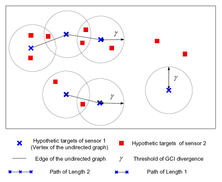
This subsection presents the construction of the undirected graph using the hypothetic objects of sensors s=1,2𝑠12s=1,2, i.e., (𝕃1,𝕃2)subscript𝕃1subscript𝕃2(\mathbb{L}_{1},\mathbb{L}_{2}), and their mutual relationship. Specifically, the constructions of vertices, edges and the paths of the undirected graph are as follows:

  • \bullet

    The vertex set V𝑉V: Each hypothetic object of sensor 1, 𝕃1subscript𝕃1\ell\in\mathbb{L}_{1} is considered as a vertex, and then all the hypothetic objects of sensor 1 form the vertex set, i.e., V=𝕃1𝑉subscript𝕃1V=\mathbb{L}_{1}.

  • \bullet

    The edge set E𝐸E: To define the relationship between each pair of vertices, firstly, for each hypothetic object 𝕃1subscript𝕃1\ell\in\mathbb{L}_{1}, extract all associated hypothetic objects from 𝕃2subscript𝕃2\mathbb{L}_{2} which fall within the gate, i.e.,

    Ψ2()={𝕃2:d(,)γ}.subscriptsuperscriptΨ2conditional-setsuperscriptsubscript𝕃2𝑑superscript𝛾\begin{split}\Psi^{(\ell)}_{2}=\{\ell^{\prime}\in\mathbb{L}_{2}:d(\ell,\ell^{\prime})\leq\gamma\}.\end{split} (50)

    If any two hypothetic objects 12𝕃1subscript1subscript2subscript𝕃1\ell_{1}\neq\ell_{2}\in\mathbb{L}_{1} have common associated hypothetic objects from sensor 2, i.e.,

    Ψ2(1)Ψ2(2),subscriptsuperscriptΨsubscript12subscriptsuperscriptΨsubscript22\begin{split}\Psi^{(\ell_{1})}_{2}\cap\Psi^{(\ell_{2})}_{2}\neq\emptyset,\end{split} (51)

    then 1subscript1\ell_{1} and 2subscript2\ell_{2} are paired to be an edge, e=(1,2)𝑒subscript1subscript2e=(\ell_{1},\ell_{2}). All pairs of hypothetic objects in 𝕃1subscript𝕃1\mathbb{L}_{1} satisfying (51) form the edge set E𝐸E,

    E={(1,2)𝕃12:12,Ψ2(1)Ψ2(2)}.E=\{(\ell_{1},\ell_{2})\in\mathbb{L}_{1}^{2}:\ell_{1}\neq\ell_{2}\ \ ,\Psi_{2}^{(\ell_{1})}\cap\Psi_{2}^{(\ell_{2})}\neq\emptyset\}. (52)
  • \bullet

    A path in G(V,E)𝐺𝑉𝐸G(V,E) is a walk in which all vertices (except possibly the first and last) are distinct, and all edges are distinct. A path of length K𝐾K in a graph is an alternating sequence of vertices and edges, i.e., 0,e0,1,e1,eK1,Ksubscript0subscript𝑒0subscript1subscript𝑒1subscript𝑒𝐾1subscript𝐾\ell_{0},e_{0},\ell_{1},e_{1}\cdots,e_{K-1},\ell_{K}, where ek1subscript𝑒𝑘1e_{k-1} connects vertices k1subscript𝑘1\ell_{k-1} and ksubscript𝑘\ell_{k}, k=1,,K𝑘1𝐾k=1,\cdots,K, 0subscript0\ell_{0} and Ksubscript𝐾\ell_{K} are the end-points, and 1,,K1subscript1subscript𝐾1\ell_{1},\cdots,\ell_{K-1} are the non-end-points.

Fig. 1 shows a sketch map for the construction of the undirected graph using the hypothetic objects of sensors 1 and 2.
Refer to caption
Figure 1: A sketch map for the construction of the undirected graph using the hypothetic objects of sensors 1 and 2.

IV-E2 Clustering based on union-find algorithm

This subsection details how to get the LIC by utilizing the undirected graph G(V,E)𝐺𝑉𝐸G(V,E). Recall (35), CIIIsubscript𝐶IIIC_{\text{III}} can be constructed as follow:

CIII={(,{}):𝕃2\(𝕃1Ψ2())}.subscript𝐶IIIconditional-setsuperscriptsuperscript\subscript𝕃2subscriptsubscript𝕃1superscriptsubscriptΨ2C_{\text{III}}=\{(\emptyset,\{\ell^{\prime}\}):\ell^{\prime}\in\mathbb{L}_{2}\backslash(\cup_{\ell\in\mathbb{L}_{1}}\Psi_{2}^{(\ell)})\}. (53)

The counterpart of sensor 2 in any cluster belonging to CIIIsubscript𝐶IIIC_{\text{III}} is a singleton whose element is an individual hypothetic object of sensor 2 having no associated hypothetic objects from 𝕃1subscript𝕃1\mathbb{L}_{1}. The choice of the singleton is to ensure the largest number of clusters.

Then, construction of CIsubscript𝐶IC_{\text{I}} and CIIsubscript𝐶IIC_{\text{II}} is the problem of seeking connected components of the undirected graph G(V,E)𝐺𝑉𝐸G(V,E). A connected component of an undirected graph is a subgraph that satisfies two conditions:

– any two vertices are connected to each other by a path;

– it is connected to no additional vertices in the supergraph.

Input: The undirected graph G(V,E)𝐺𝑉𝐸G(V,E);
for each V𝑉\ell\in V do
      Makeset()(\ell)
end for
for each (1,2)Esubscript1subscript2𝐸(\ell_{1},\ell_{2})\in E do
       if Find(1)subscript1absent(\ell_{1})\neqFind(2)subscript2(\ell_{2})  then
            Union(1,2)subscript1subscript2(\ell_{1},\ell_{2})
       end if
      
end for
Output: Connected components of G𝐺G.
Algorithm 1 Union_Find_Algorithm.

Dynamic tracking of the connected components of a graph as vertices and edges is a straightforward application of disjoint-set data structures [39]. A disjoint-set data structure maintains a dynamic collection of disjoint subsets that together cover the whole set. The underline data structure of each set is typically a rooted-tree, identified by a representative element of the set, also called the parent node. The two main operations are to Find which set a given element belongs to by locating its father node and to replace two existing sets with their Union. We outline a primary Union-Find algorithm from the viewpoint of its use in finding connected components of the graph G(V,E)𝐺𝑉𝐸G(V,E) as shown in Algorithm 1.

The procedure of seeking connected components can be expanded as follows. Firstly, initialize |V|𝑉|V| trees, each of which takes an individual element of V𝑉V as the parent node and a rank of 0, which is exactly the operation Makeset. Then, for each edge (1,2)Esubscript1subscript2𝐸(\ell_{1},\ell_{2})\in E, find their parent nodes through the operation Find. If parent nodes of 1subscript1\ell_{1} and 2subscript2\ell_{2} are the same, i.e. if they have already been in the same tree, then no operation is needed; otherwise, merge the trees which 1subscript1\ell_{1} and 2subscript2\ell_{2} belong to, respectively, using the operation Union. Finally, we get all the connected components of G(V,E)𝐺𝑉𝐸G(V,E), denoted by Gg(Vg,Eg),g=1,,NGformulae-sequencesubscript𝐺𝑔subscript𝑉𝑔subscript𝐸𝑔𝑔1subscript𝑁𝐺G_{g}(V_{g},E_{g}),g=1,\cdots,N_{G}.

Accordingly, 𝕃1subscript𝕃1\mathbb{L}_{1} is partitioned into NGsubscript𝑁𝐺N_{G} disjoint subsets, i.e.,

𝕃1,g=Vg,g=1,,NG;formulae-sequencesubscript𝕃1𝑔subscript𝑉𝑔𝑔1subscript𝑁𝐺\mathbb{L}_{1,g}=V_{g},g=1,\cdots,N_{G}; (54)

and for each 𝕃1,gsubscript𝕃1𝑔\mathbb{L}_{1,g}, all the associated hypothetic objects from sensor 2 are merged, i.e.,

𝕃2,g=𝕃1,gΨ2().subscript𝕃2𝑔subscriptsubscript𝕃1𝑔superscriptsubscriptΨ2\mathbb{L}_{2,g}=\cup_{\ell\in\mathbb{L}_{1,g}}\Psi_{2}^{(\ell)}. (55)

Then each pair of 𝕃1,gsubscript𝕃1𝑔\mathbb{L}_{1,g} and 𝕃2,gsubscript𝕃2𝑔\mathbb{L}_{2,g} forms an isolated cluster 𝒞g=(𝕃1,g,𝕃2,g)subscript𝒞𝑔subscript𝕃1𝑔subscript𝕃2𝑔\mathcal{C}_{g}=(\mathbb{L}_{1,g},\mathbb{L}_{2,g}), and all the isolated clusters form the clusters of types CICIIsubscript𝐶Isubscript𝐶IIC_{\text{I}}\cup C_{\text{II}} in the finalized LIC,

CICII={𝒞1,,𝒞NG}.subscript𝐶Isubscript𝐶IIsubscript𝒞1subscript𝒞subscript𝑁𝐺C_{\text{I}}\cup C_{\text{II}}=\{\mathcal{C}_{1},\cdots,\mathcal{C}_{N_{G}}\}. (56)
Remark 8.

Any vertex satisfying Ψ2()=superscriptsubscriptΨ2\Psi_{2}^{(\ell)}=\emptyset is a connected component, since it cannot be linked to any other vertex. Hence, it is easy to separate CIIsubscript𝐶IIC_{\emph{II}} from the union in (56), i.e.,

CII={({},):Ψ2()=,𝕃1},subscript𝐶IIconditional-setformulae-sequencesuperscriptsubscriptΨ2subscript𝕃1C_{\emph{II}}=\{(\{\ell\},\emptyset):\Psi_{2}^{(\ell)}=\emptyset,\ell\in\mathbb{L}_{1}\}, (57)

for which the counterpart of sensor 1 in any cluster is a singleton whose element is an individual hypothetic object having no associated hypothetic object from sensor 2.

Proposition 4.

The union C=CICIICIII𝐶subscript𝐶Isubscript𝐶IIsubscript𝐶IIIC=C_{\emph{I}}\cup C_{\emph{II}}\cup C_{\emph{III}} with CIsubscript𝐶IC_{\emph{I}}, CIIsubscript𝐶IIC_{\emph{II}} and CIIIsubscript𝐶IIIC_{\emph{III}}, respectively, given in (56) and (53) is the LIC.

The proof of Proposition 4 is given in Appendix D. Proposition 4 ensures that one can obtain a unique LIC using the disjoint-set data structure-based fast clustering, thus building exactly the independence approximation of form (36).

Remark 9.

Algorithm 1 only shows the primary Union-Find algorithm. Actually, there exist many classical theoretical studies providing enhanced implementations of the Union-Find algorithm, including Link-by-Rank or Link-by-Size for the union operation and Path-Compression, Path-Splitting, or Path-Halving for the find operation [40, 41]. The worst-case time complexity of the enhanced union-find algorithm is 𝒪(n+mα(m,n))𝒪𝑛𝑚𝛼𝑚𝑛\mathcal{O}(n+m\alpha(m,n)) for any combination of m𝑚m Makeset, Union, and Find operations on n𝑛n elements, where α𝛼\alpha is the very slowly growing inverse of Ackermann¡¯s function.

IV-F Summary

The combination of the independence approximation (36) and Proposition 4 enables a computationally efficient GCI-MB fusion algorithm. The fast clustering algorithm is employed at an early stage to form the LIC and thus obtain the approximated density. Then GCI-MB fusion is performed within each smaller clusters of LIC independently and parallelizablly by exploiting the structure of the approximated density. We refer to this fusion method as the parallelizable GCI-MB (P-GCI-MB) to emphasize its intuitive implementation structure.

Note that Proposition 4 also ensures that the only approximation error arises from discarding the inter-cluster hypotheses. The analysis in Proposition 3 further shows that as long as the clustering threshold is sufficiently large, the approximation error is negligible. Hence, the proposed P-GCI-MB method is able to reduce the computational expense as well as memory requirements with slight and bounded error.

Remark 10.

Theoretically in the worst case where all hypothetic objects are in close proximity, it may not be possible to partition objects into smaller clusters. In this case, the complexity of P-GCI-MB is the same as that of the original GCI-MB fusion.

V Implementation of P-GCI-MB Fusion

In this section, two common implementation approaches of the P-GCI-MB Fusion, i.e., GM and SMC approaches are presented. The GM approach is suitable for the case of linear or weak non-linear models, while the SMC approach is general enough for both linear and non-linear models. Compared with SMC approach, the advantage of GM approach lies on its lower load in terms of both local (in-node) computations and inter-node data communications.

V-A The GM implementation

At the first step of the P-GCI-MB fusion, the quantities needed to calculate are the distances (i.e., GCI divergences) d(,),(,)𝕃1×𝕃2𝑑superscriptsuperscriptsubscript𝕃1subscript𝕃2d(\ell,\ell^{\prime}),(\ell,\ell^{\prime})\in\mathbb{L}_{1}\times\mathbb{L}_{2} in (24). Then, we need to calculate pω(,θ)superscriptsubscript𝑝𝜔𝜃p_{\omega}^{(\ell,\theta)} and w(I1,θ)superscript𝑤subscript𝐼1𝜃w^{(I_{1},\theta)} for each fusion hypothesis (I1,θ)subscript𝐼1𝜃(I_{1},\theta) of each cluster. Since their calculations involve the integrations which do not have closed form solutions in general, we resort to GM realization. Having the results of quantities d(,)𝑑superscriptd(\ell,\ell^{\prime}), pω(,θ)superscriptsubscript𝑝𝜔𝜃p_{\omega}^{(\ell,\theta)} and w(I1,θ)superscript𝑤subscript𝐼1𝜃w^{(I_{1},\theta)}, other terms required in P-GCI-MB can be calculated accordingly.

V-A1 GM evaluation of d(,)𝑑superscriptd(\ell,\ell^{\prime})

The pairwise distances between hypothetic tracks of two sensors need to be computed first since they are the inputs to the clustering algorithm in order to obtain the LIC. Using the GM approximation, the posterior of the s𝑠s-th local sensor can be expressed as {(rs(),ps()(x))}𝕃ssubscriptsuperscriptsubscript𝑟𝑠superscriptsubscript𝑝𝑠𝑥subscript𝕃𝑠\{(r_{s}^{(\ell)},p_{s}^{(\ell)}(x))\}_{\ell\in\mathbb{L}_{s}}, with each probability density ps()(x)superscriptsubscript𝑝𝑠𝑥p_{s}^{(\ell)}(x) being represented as a mixture of Gaussian components:

ps()(x)=j=1Js()αs(,j)𝒩(x;ms(,j),Ps(,j))superscriptsubscript𝑝𝑠𝑥superscriptsubscript𝑗1superscriptsubscript𝐽𝑠superscriptsubscript𝛼𝑠𝑗𝒩𝑥superscriptsubscript𝑚𝑠𝑗superscriptsubscript𝑃𝑠𝑗\begin{split}p_{s}^{(\ell)}(x)={\sum}_{j=1}^{J_{s}^{(\ell)}}\alpha_{s}^{(\ell,j)}\mathcal{N}\left(x;m_{s}^{(\ell,j)},P_{s}^{(\ell,j)}\right)\end{split} (58)

where 𝒩(x;m,P)𝒩𝑥𝑚𝑃\mathcal{N}\left(x;m,P\right) denotes a Gaussian density with mean m𝑚m and covariance P𝑃P, Js()superscriptsubscript𝐽𝑠J_{s}^{(\ell)} is the number of Gaussian components for the \ell-th Bernoulli component, αs(,j)superscriptsubscript𝛼𝑠𝑗\alpha_{s}^{(\ell,j)} is the weight of the j𝑗j-th Gaussian component for the \ell-th Bernoulli component.

Observing (19) and (24), we find that calculation of both pω(,θ)superscriptsubscript𝑝𝜔𝜃p_{\omega}^{(\ell,\theta)} and d(,)𝑑superscriptd(\ell,\ell^{\prime}) involves integrating the Gaussian mixture in (58) taken to the power of ωssubscript𝜔𝑠\omega_{s}, which in general has no analytical solution. In this respect, we adopt the principled approximation suggested by Battistelli et al.[7] and Julier [42],

[j=1Js()αs(,j)𝒩(x;ms(,j),Ps(,j))]ωsj=1Js()[αs(,j)𝒩(x;ms(,j),Ps(,j))]ωsapproximately-equals-or-equalssuperscriptdelimited-[]superscriptsubscript𝑗1superscriptsubscript𝐽𝑠superscriptsubscript𝛼𝑠𝑗𝒩𝑥superscriptsubscript𝑚𝑠𝑗superscriptsubscript𝑃𝑠𝑗subscript𝜔𝑠superscriptsubscript𝑗1superscriptsubscript𝐽𝑠superscriptdelimited-[]superscriptsubscript𝛼𝑠𝑗𝒩𝑥superscriptsubscript𝑚𝑠𝑗superscriptsubscript𝑃𝑠𝑗subscript𝜔𝑠\begin{split}&\left[{\sum}_{j=1}^{J_{s}^{(\ell)}}\alpha_{s}^{(\ell,j)}\mathcal{N}\left(x;m_{s}^{(\ell,j)},P_{s}^{(\ell,j)}\right)\right]^{\omega_{s}}\\ &\hskip 48.36967pt\approxeq{\sum}_{j=1}^{J_{s}^{(\ell)}}\left[\alpha_{s}^{(\ell,j)}\mathcal{N}\left(x;m_{s}^{(\ell,j)},P_{s}^{(\ell,j)}\right)\right]^{\omega_{s}}\end{split} (59)

with the condition that the Gaussian components of ps()(x)superscriptsubscript𝑝𝑠𝑥p_{s}^{(\ell)}(x) are well separated relatively to their corresponding covariances. If this condition is not satisfied, one can either perform merging before fusion (this is possible, since, for an MB, each probability density ps()()superscriptsubscript𝑝𝑠p_{s}^{(\ell)}(\cdot) is corresponding to a single hypothetic object) or use other approximations, e.g., replacing the GM representation by a sigma-point approximation [43].

Using (59), the term p1()(x)ω1p2()(x)ω2superscriptsubscript𝑝1superscript𝑥subscript𝜔1superscriptsubscript𝑝2superscriptsuperscript𝑥subscript𝜔2p_{1}^{(\ell)}(x)^{\omega_{1}}p_{2}^{(\ell^{\prime})}(x)^{\omega_{2}} is expressed as

p1()(x)ω1p2()(x)ω2=j=1J1()j=1J2()αω(,j,,j)𝒩(x;m12(,j,,j),P12(,j,,j))superscriptsubscript𝑝1superscript𝑥subscript𝜔1superscriptsubscript𝑝2superscriptsuperscript𝑥subscript𝜔2superscriptsubscript𝑗1superscriptsubscript𝐽1superscriptsubscriptsuperscript𝑗1superscriptsubscript𝐽2superscriptsuperscriptsubscript𝛼𝜔𝑗superscriptsuperscript𝑗𝒩𝑥superscriptsubscript𝑚12𝑗superscriptsuperscript𝑗superscriptsubscript𝑃12𝑗superscriptsuperscript𝑗\begin{split}&p_{1}^{(\ell)}(x)^{\omega_{1}}p_{2}^{(\ell^{\prime})}(x)^{\omega_{2}}\\ &\hskip 17.07164pt=\sum_{j=1}^{J_{1}^{(\ell)}}\sum_{j^{\prime}=1}^{J_{2}^{(\ell^{\prime})}}\alpha_{\omega}^{(\ell,j,\ell^{\prime},j^{\prime})}\mathcal{N}\left(x;m_{12}^{(\ell,j,\ell^{\prime},j^{\prime})},P_{12}^{(\ell,j,\ell^{\prime},j^{\prime})}\right)\end{split} (60)

where

αω(,j,,j)=superscriptsubscript𝛼𝜔𝑗superscriptsuperscript𝑗absent\displaystyle\alpha_{\omega}^{(\ell,j,\ell^{\prime},j^{\prime})}\!= α~ω(,j,,j)𝒩(m1(,j)m2(,j);0,P1(,j)ω1+P2(,j)ω2)superscriptsubscript~𝛼𝜔𝑗superscriptsuperscript𝑗𝒩superscriptsubscript𝑚1𝑗superscriptsubscript𝑚2superscriptsuperscript𝑗0superscriptsubscript𝑃1𝑗subscript𝜔1superscriptsubscript𝑃2superscriptsuperscript𝑗subscript𝜔2\displaystyle\widetilde{\alpha}_{\omega}^{(\ell,j,\ell^{\prime},j^{\prime})}\mathcal{N}\!\!\left(\!\!m_{1}^{(\ell,j)}\!\!-\!m_{2}^{(\ell^{\prime},j^{\prime})};0,\!\frac{P_{1}^{(\ell,j)}}{\omega_{1}}\!\!+\!\!\frac{P_{2}^{(\ell^{\prime},j^{\prime})}}{\omega_{2}}\!\!\right) (61)
P12(,j,,j)=superscriptsubscript𝑃12𝑗superscriptsuperscript𝑗absent\displaystyle P_{12}^{(\ell,j,\ell^{\prime},j^{\prime})}\!=\! ([P1(,j)]1+[P2(θ(),j)]1)1superscriptsuperscriptdelimited-[]superscriptsubscript𝑃1𝑗1superscriptdelimited-[]superscriptsubscript𝑃2𝜃superscript𝑗11\displaystyle\left([P_{1}^{(\ell,j)}]^{-1}+[P_{2}^{(\theta(\ell),j^{\prime})}]^{-1}\right)^{-1} (62)
m12(,j,,j)=superscriptsubscript𝑚12𝑗superscriptsuperscript𝑗absent\displaystyle m_{12}^{(\ell,j,\ell^{\prime},j^{\prime})}\!= P12(,j)([P1(,j)]1m1(,j)+[P2(,j)]1m2(,j))superscriptsubscript𝑃12𝑗superscriptdelimited-[]superscriptsubscript𝑃1𝑗1superscriptsubscript𝑚1𝑗superscriptdelimited-[]superscriptsubscript𝑃2superscriptsuperscript𝑗1superscriptsubscript𝑚2superscriptsuperscript𝑗\displaystyle P_{12}^{(\ell,j)}\left([P_{1}^{(\ell,j)}]^{-\!1}m_{1}^{(\ell,j)}\!\!+\![P_{2}^{(\ell^{\prime},j^{\prime})}]^{-\!1}m_{2}^{(\ell^{\prime},j^{\prime})}\right) (63)

with

α~ω(,j,,j)superscriptsubscript~𝛼𝜔𝑗superscriptsuperscript𝑗\displaystyle\widetilde{\alpha}_{\omega}^{(\ell,j,\ell^{\prime},j^{\prime})} =(α1(,j))ω1(α2(,j))ω2ρ(P1(,j),ω1)ρ(P2(,j),ω2)absentsuperscriptsuperscriptsubscript𝛼1𝑗subscript𝜔1superscriptsuperscriptsubscript𝛼2superscriptsuperscript𝑗subscript𝜔2𝜌superscriptsubscript𝑃1𝑗subscript𝜔1𝜌superscriptsubscript𝑃2superscriptsuperscript𝑗subscript𝜔2\displaystyle=(\!\alpha_{1}^{(\ell,j)}\!)^{\omega_{1}}(\!\alpha_{2}^{(\ell^{\prime},j^{\prime})}\!)^{\omega_{2}}\!\rho(P_{1}^{(\ell,j)}\!,\!\omega_{1})\!\rho(P_{2}^{(\ell^{\prime},j^{\prime})}\!,\!\omega_{2}) (64)
ρ(P,ω)𝜌𝑃𝜔\displaystyle\rho(P,\omega) =det[2πPω1](det[2πP])ω.absentdelimited-[]2𝜋𝑃superscript𝜔1superscriptdelimited-[]2𝜋𝑃𝜔\displaystyle=\sqrt{\det[2\pi P\omega^{-1}](\det[2\pi P])^{-\omega}}. (65)

Substituting (LABEL:density_Bernoulli) into (24) and performing integration, we have

d(,)=log(j=1J1()j=1J2()αω(,j,,j)).𝑑superscriptsuperscriptsubscript𝑗1superscriptsubscript𝐽1superscriptsubscriptsuperscript𝑗1superscriptsubscript𝐽2superscriptsuperscriptsubscript𝛼𝜔𝑗superscript𝑗d(\ell,\ell^{\prime})=-\log\left({\sum}_{j=1}^{J_{1}^{(\ell)}}{\sum}_{j^{\prime}=1}^{J_{2}^{(\ell^{\prime})}}\alpha_{\omega}^{(\ell,j,\ell,j^{\prime})}\right). (66)

V-A2 Evaluation of pω(,θ)()superscriptsubscript𝑝𝜔𝜃p_{\omega}^{(\ell,\theta)}(\cdot) and wω(I1,θ)superscriptsubscript𝑤𝜔subscript𝐼1𝜃w_{\omega}^{(I_{1},\theta)}

After discovering the LIC based on the pairwise distances (66), for each cluster g𝑔g, let 𝕃1,gsubscript𝕃1𝑔\ell\in\mathbb{L}_{1,g}, θΘg𝜃subscriptΘ𝑔\theta\in\Theta_{g}. Substituting =θ()superscript𝜃\ell^{\prime}=\theta(\ell) into (LABEL:density_Bernoulli), we can obtain the numerator of density pω(,θ)()superscriptsubscript𝑝𝜔𝜃p_{\omega}^{(\ell,\theta)}(\cdot) as

p1()(x)ω1p2(θ())(x)ω2=j=1J1()j=1J2(θ())αω(,j,θ(),j)𝒩(x;m12(,j,θ(),j),P12(,j,θ(),j)).superscriptsubscript𝑝1superscript𝑥subscript𝜔1superscriptsubscript𝑝2𝜃superscript𝑥subscript𝜔2superscriptsubscript𝑗1superscriptsubscript𝐽1superscriptsubscriptsuperscript𝑗1superscriptsubscript𝐽2𝜃superscriptsubscript𝛼𝜔𝑗𝜃superscript𝑗𝒩𝑥superscriptsubscript𝑚12𝑗𝜃superscript𝑗superscriptsubscript𝑃12𝑗𝜃superscript𝑗\begin{split}&p_{1}^{(\ell)}(x)^{\omega_{1}}p_{2}^{(\theta(\ell))}(x)^{\omega_{2}}\\ =&\sum_{j=1}^{J_{1}^{(\ell)}}\sum_{j^{\prime}=1}^{J_{2}^{(\theta(\ell))}}\alpha_{\omega}^{(\ell,j,\theta(\ell),j^{\prime})}\mathcal{N}\left(x;m_{12}^{(\ell,j,\theta(\ell),j^{\prime})},\!P_{12}^{(\ell,j,\theta(\ell),j^{\prime})}\right).\end{split} (67)

Further, the parameter Zω(,θ)superscriptsubscript𝑍𝜔𝜃Z_{\omega}^{(\ell,\theta)} in (16) can be computed by

Zω(,θ)=exp(d(,θ()).\begin{split}Z_{\omega}^{(\ell,\theta)}=\exp(-d(\ell,\theta(\ell)).\end{split} (68)

By substituting (68) and (LABEL:density_Bernoulli_theta) into (13), the parameter pω(,θ())superscriptsubscript𝑝𝜔𝜃p_{\omega}^{(\ell,\theta(\ell))} turns out to be

pω(,θ())(x)=p1()(x)ω1p2(θ())(x)ω2Zω(,θ)=j=1J1()j=1J2(θ())αω(,j,θ(),j)𝒩(x;m12(,j,θ(),j),P12(,j,θ(),j))exp(d(,θ()).\begin{split}&p_{\omega}^{(\ell,\theta(\ell))}(x)=\frac{p_{1}^{(\ell)}(x)^{\omega_{1}}p_{2}^{(\theta(\ell))}(x)^{\omega_{2}}}{Z_{\omega}^{(\ell,\theta)}}\\ =&\frac{\sum_{j=1}^{J_{1}^{(\ell)}}\sum_{j^{\prime}=1}^{J_{2}^{(\theta(\ell))}}\alpha_{\omega}^{(\ell,j,\theta(\ell),j^{\prime})}\mathcal{N}\left(x;m_{12}^{(\ell,j,\theta(\ell),j^{\prime})},P_{12}^{(\ell,j,\theta(\ell),j^{\prime})}\right)}{\exp(-d(\ell,\theta(\ell))}.\end{split} (69)

By combing (68) with (14), (15), the un-normalized weight w~ω(I1,θ)superscriptsubscript~𝑤𝜔subscript𝐼1𝜃\widetilde{w}_{\omega}^{(I_{1},\theta)} for each (I1,θ)(𝕃1,g)×Θg(I1)subscript𝐼1𝜃subscript𝕃1𝑔subscriptΘ𝑔subscript𝐼1(I_{1},\theta)\in\mathcal{F}(\mathbb{L}_{1,g})\times\Theta_{g}(I_{1}) and the normalization constant ηωsubscript𝜂𝜔\eta_{\omega} are calculated as

w~ω(I1,θ)superscriptsubscript~𝑤𝜔subscript𝐼1𝜃\displaystyle\widetilde{w}_{\omega}^{(I_{1},\theta)} =(Q1I1)ω1(Q2θ(I1))ω2I1exp(d(,θ())\displaystyle=\left(Q_{1}^{I_{1}}\right)^{\omega_{1}}\left(Q_{2}^{\theta(I_{1})}\right)^{\omega_{2}}\prod_{\ell\in I_{1}}\exp(-d(\ell,\theta(\ell)) (70)
ηωsubscript𝜂𝜔\displaystyle\!\!\eta_{\omega} =I1(𝕃1)θΘg(I1)w~ω(I1,θ).absentsubscriptsubscript𝐼1subscript𝕃1subscript𝜃subscriptΘ𝑔subscript𝐼1superscriptsubscript~𝑤𝜔subscript𝐼1𝜃\displaystyle={\sum}_{I_{1}\in\mathcal{F}(\mathbb{L}_{1})}{\sum}_{\theta\in\Theta_{g}(I_{1})}\widetilde{w}_{\omega}^{(I_{1},\theta)}. (71)

Thus, by substituting (70) and (71) into (12), the GM representation of the normalized weight wω(I1,θ)superscriptsubscript𝑤𝜔subscript𝐼1𝜃w_{\omega}^{(I_{1},\theta)} is calculated.

V-B SMC implementation

The SMC realization of GCI-MB was previously given in [27]. Since the P-GCI-MB fusion contains parallelizable GCI-MB fusion operations with several smaller clusters, the SMC implementation of P-GCI-MB fusion for each cluster is straightforward and similar to [27]. As for the pair-wise distances d(,),(,)𝕃1×𝕃2𝑑superscriptsuperscriptsubscript𝕃1subscript𝕃2d(\ell,\ell^{\prime}),(\ell,\ell^{\prime})\in\mathbb{L}_{1}\times\mathbb{L}_{2} which are the outputs of the clustering algorithm, one can also refer to the SMC evaluation of Zω(,θ)superscriptsubscript𝑍𝜔𝜃Z_{\omega}^{(\ell,\theta)} given in [27], since the distance d(,θ())𝑑𝜃d(\ell,\theta(\ell)) is functionally related to Zω(,θ)superscriptsubscript𝑍𝜔𝜃Z_{\omega}^{(\ell,\theta)} following (68).

V-C Pseudo-code of P-GCI-MB fusion

The psedo-code of P-GCI-MB fusion are given in Algorithms 2 and 3. Specifically, Algorithm 2 forms the LIC using the disjoint-set data structure; and Algorithm 3 describes the whole fusion algorithm in a two-sensor case. This implementation can also be easily extended to Ns2subscript𝑁𝑠2N_{s}\geqslant 2 sensors by sequentially applying the pairwise fusion (18) and (19) under each clusters Ns1subscript𝑁𝑠1N_{s}-1 times, where the ordering of pairwise fusions is irrelevant. Similar mechanism has been used in CPHD filters and LMB filters based GCI fusions [7, 35]. In addition, by exploiting the consensus approach, the P-GCI-MB fusion can be also implemented in a fully distributed way, similar to [7]. The consensus based P-GCI-MB fusion achieves the global P-GCI-MB fusion over the whole network by iterating the local fusion steps among neighbouring sensor nodes.

Input: πs={(rs(),ps()())}𝕃ssubscript𝜋𝑠subscriptsuperscriptsubscript𝑟𝑠superscriptsubscript𝑝𝑠subscript𝕃𝑠\pi_{s}=\!\{(r_{s}^{(\ell)},p_{s}^{(\ell)}(\cdot))\}_{\ell\in\mathbb{L}_{s}} from nodes s=1,2𝑠12s=1,2 Output: The LIC C𝐶{C} and the distance matrix Dωsubscript𝐷𝜔D_{\omega} function Clustering_Function (π1,π2)subscript𝜋1subscript𝜋2(\pi_{1},\pi_{2}) Define a undirected graph, G=(V,E)𝐺𝑉𝐸G=(V,E) with V=𝕃1𝑉subscript𝕃1V=\mathbb{L}_{1};
Initialize the set of edges, E=𝐸E=\emptyset;
Initialize a distance matrix Dω=subscript𝐷𝜔D_{\omega}=\emptyset with |𝕃1|subscript𝕃1|\mathbb{L}_{1}| columns and |𝕃2|subscript𝕃2|\mathbb{L}_{2}| rows;
Initialize the row number of Dωsubscript𝐷𝜔D_{\omega}, i=0𝑖0i=0;
Initialize the column number of Dωsubscript𝐷𝜔D_{\omega}, j=0𝑗0j=0;
for =1:|𝕃1|:1subscript𝕃1\ell=1:|\mathbb{L}_{1}| do
      Ψ2()=superscriptsubscriptΨ2\Psi_{2}^{(\ell)}=\emptyset;
       for =1:|𝕃2|:superscript1subscript𝕃2\ell^{\prime}=1:|\mathbb{L}_{2}| do
            Evaluate the distance parameter d(,)𝑑superscriptd(\ell,\ell^{\prime}); contains-as-subgroup\rhd(24);
             if d(,)<Γ𝑑superscriptΓd(\ell,\ell^{\prime})<\Gamma then
                  Ψ2()=Ψ2(){}superscriptsubscriptΨ2superscriptsubscriptΨ2superscript\Psi_{2}^{(\ell)}=\Psi_{2}^{(\ell)}\cup\{\ell^{\prime}\} ;
                  
             end if
            Dω[i+1,j+1]=d(,)subscript𝐷𝜔𝑖1𝑗1𝑑superscriptD_{\omega}[i+1,j+1]=d(\ell,\ell^{\prime});
             i=:i+1i=:i+1
       end for
      if >11\ell>1 then
             for temp=1::subscripttemp1\ell_{\text{temp}}=1:\ell do
                  if Ψ2()Ψ2(temp)superscriptsubscriptΨ2superscriptsubscriptΨ2subscripttemp\Psi_{2}^{{(\ell)}}\cap\Psi_{2}^{(\ell_{\text{temp}})}\neq\emptyset then
                        E=E{(,temp)}𝐸𝐸subscripttempE=E\cup\{(\ell,\ell_{\text{temp}})\}
                   end if
                  
             end for
            
       end if
      j=:j+1j=:j+1
end for
[𝕃1,1,,𝕃1,N𝒞]=Union_Find_Algorithm(G(V,E))subscript𝕃11subscript𝕃1subscript𝑁𝒞Union_Find_Algorithm𝐺𝑉𝐸[\mathbb{L}_{1,1},\cdots,\mathbb{L}_{1,N_{\mathcal{C}}}]=\text{Union\_Find\_Algorithm}(G(V,E));
for g=1:N𝒞:𝑔1subscript𝑁𝒞g=1:N_{\mathcal{C}} do
      𝕃2,g=𝕃1,gΨ2()subscript𝕃2𝑔subscriptsubscript𝕃1𝑔superscriptsubscriptΨ2\mathbb{L}_{2,g}=\cup_{\ell\in\mathbb{L}_{1,g}}\Psi_{2}^{(\ell)};
      
end for
Return: The LIC C={(𝕃1,g,𝕃2,g)}g=1N𝒞𝐶superscriptsubscriptsubscript𝕃1𝑔subscript𝕃2𝑔𝑔1subscript𝑁𝒞{C}=\{(\mathbb{L}_{1,g},\mathbb{L}_{2,g})\}_{g=1}^{N_{\mathcal{C}}} and Dωsubscript𝐷𝜔D_{\omega}.
Algorithm 2 Pseudo-code of the Clustering_Function.
Input: πs={(rs(),ps()())}𝕃ssubscript𝜋𝑠subscriptsuperscriptsubscript𝑟𝑠superscriptsubscript𝑝𝑠subscript𝕃𝑠\pi_{s}=\!\{(r_{s}^{(\ell)},p_{s}^{(\ell)}(\cdot))\}_{\ell\in\mathbb{L}_{s}} from nodes s=1,2𝑠12s=1,2 Output: The fused density πω={(rω(),pω()())}𝕃ωsubscript𝜋𝜔subscriptsuperscriptsubscript𝑟𝜔superscriptsubscript𝑝𝜔subscript𝕃𝜔\pi_{\omega}=\!\{(r_{\omega}^{(\ell)},p_{\omega}^{(\ell)}(\cdot))\}_{\ell\in\mathbb{L}_{\omega}} function: P_GCI_MB_Fusion(π1,π2)subscript𝜋1subscript𝜋2(\pi_{1},\pi_{2}) C=𝐶absent{C}= Clustering_Function (π1,π2)subscript𝜋1subscript𝜋2(\pi_{1},\pi_{2});
Initialize the fused MB parameter set, πω=subscript𝜋𝜔\pi_{\omega}=\emptyset;
for g=1:N𝒞:𝑔1subscript𝑁𝒞g=1:N_{\mathcal{C}} do
      Create the map space Θg={θg:𝕃1,g𝕃2,g\Theta_{g}=\{\theta_{g}:\mathbb{L}_{1,g}\rightarrow\mathbb{L}_{2,g}};
       for I1(𝕃1,g)subscript𝐼1subscript𝕃1𝑔I_{1}\in\mathcal{F}(\mathbb{L}_{1,g}) do
             for θΘg(I1)𝜃subscriptΘ𝑔subscript𝐼1\theta\in\Theta_{g}(I_{1}) do
                   for I1subscript𝐼1\ell\in I_{1} do
                         Find the quantity dω(,θ())superscriptsubscript𝑑𝜔𝜃d_{\omega}^{(\ell,\theta(\ell))} in Dωsubscript𝐷𝜔D_{\omega};
                         Calculate the quantity Zω(,θ)superscriptsubscript𝑍𝜔𝜃Z_{\omega}^{(\ell,\theta)}; contains-as-subgroup\rhd(68) Evaluate the quantity pω(,θ)(x)superscriptsubscript𝑝𝜔𝜃𝑥p_{\omega}^{(\ell,\theta)}(x); contains-as-subgroup\rhd(LABEL:fuse-p-gm)
                   end for
                  Calculate the weight w~ω(I1,θ)superscriptsubscript~𝑤𝜔subscript𝐼1𝜃\widetilde{w}_{\omega}^{(I_{1},\theta)}; contains-as-subgroup\rhd(70)
             end for
            
       end for
      Calculate normalized factor η𝜂\eta; contains-as-subgroup\rhd(71)
      Normalize the weight w~ω(I1,θ)superscriptsubscript~𝑤𝜔subscript𝐼1𝜃\widetilde{w}_{\omega}^{(I_{1},\theta)}; contains-as-subgroup\rhd(12)
      for 𝕃1,gsubscript𝕃1𝑔\ell\in\mathbb{L}_{1,g} do
             Calculate the MB parameter r()superscript𝑟r^{(\ell)}; contains-as-subgroup\rhd(18) Calculate the MB parameter p()(x)superscript𝑝𝑥p^{(\ell)}(x); contains-as-subgroup\rhd(19)
       end for
      πω=πω{(r(),p()(x))}𝕃1,gsubscript𝜋𝜔subscript𝜋𝜔subscriptsuperscript𝑟superscript𝑝𝑥subscript𝕃1𝑔\pi_{\omega}=\pi_{\omega}\cup\{(r^{(\ell)},p^{(\ell)}(x))\}_{\ell\in\mathbb{L}_{1,g}};
      
end for
return: πωsubscript𝜋𝜔\pi_{\omega}.
Algorithm 3 Pseudo-code of the GM P-GCI-MB fusion

V-D Computational complexity

The computational complexity of P-GCI-MB is then analyzed by comparison with the GCI fusion of the CPHD filter (GCI-CPHD) [7, 5], considering both GM and SMC implementations. For the GM implementation, assume that the probability density of each Bernoulli component of each local MB filter is represented by a mixture of J𝐽J Gaussian components, and the location density of each local CPHD filter by a mixture of nmaxJsubscript𝑛𝐽n_{\max}J Gaussian components, where nmaxsubscript𝑛n_{\max} denotes the maximum number of objects. Similarly, for the SMC implementation, assume that the probability density of each Bernoulli component of each local MB filter is approximated by Npsubscript𝑁𝑝N_{p} particles, while the location density of each local CPHD filter is approximated by nmaxNpsubscript𝑛subscript𝑁𝑝n_{\max}N_{p} particles. Further, assume that the dimension of the single-object state x𝑥x is Ndsubscript𝑁𝑑N_{d}.

The computational complexity of P-GCI-MB mainly consists of the following four parts:

  1. 1.

    Computation of pairwise distances between hypothetic objects of two sensors:

    \bullet GM implementation – 𝒪(Lmax2J2Nd3)𝒪subscriptsuperscript𝐿2superscript𝐽2superscriptsubscript𝑁𝑑3\mathcal{O}\left(L^{2}_{\max}J^{2}N_{d}^{3}\right);

    \bullet SMC implementation – 𝒪(Lmax2NpNd3)𝒪subscriptsuperscript𝐿2subscript𝑁𝑝superscriptsubscript𝑁𝑑3\mathcal{O}\left(L^{2}_{\max}N_{p}N_{d}^{3}\right);

    where Lmax=max{|𝕃1|,|𝕃2|}subscript𝐿subscript𝕃1subscript𝕃2L_{\max}=\max\{|\mathbb{L}_{1}|,|\mathbb{L}_{2}|\};

  2. 2.

    Finding the LIC: 𝒪(|E|+Lmaxα(|E|,Lmax))𝒪𝐸subscript𝐿𝛼𝐸subscript𝐿\mathcal{O}\left(|E|+L_{\max}\alpha(|E|,L_{\max})\right), where |E|=Lmax(Lmax1)2𝐸subscript𝐿subscript𝐿12|E|=\frac{L_{\max}(L_{\max}-1)}{2} in the worst case;

  3. 3.

    Calculation of the fused single-object densities p(,)()superscript𝑝superscriptp^{(\ell,\ell^{\prime})}(\cdot):

    \bullet GM implementation – 𝒪(N𝒞I[LmaxC]2J2Nd3)𝒪subscript𝑁subscript𝒞Isuperscriptdelimited-[]subscriptsuperscript𝐿𝐶2superscript𝐽2superscriptsubscript𝑁𝑑3\mathcal{O}(N_{\mathcal{C}_{\text{I}}}[L^{C}_{\max}]^{2}J^{2}N_{d}^{3});

    \bullet SMC implementation – 𝒪(N𝒞I[LmaxC]2NpNd3)𝒪subscript𝑁subscript𝒞Isuperscriptdelimited-[]subscriptsuperscript𝐿𝐶2subscript𝑁𝑝superscriptsubscript𝑁𝑑3\mathcal{O}(N_{\mathcal{C}_{\text{I}}}[L^{C}_{\max}]^{2}N_{p}N_{d}^{3});

    where LmaxC=maxg:𝒞gCI|𝕃1,g|subscriptsuperscript𝐿𝐶subscript:𝑔subscript𝒞𝑔subscript𝐶Isubscript𝕃1𝑔L^{C}_{\max}=\max_{g:\mathcal{C}_{g}\in C_{\text{I}}}|\mathbb{L}_{1,g}| denotes the number of hypothetic objects in the largest cluster;

  4. 4.

    Calculation of the weight w~ω(I1,θ)superscriptsubscript~𝑤𝜔subscript𝐼1𝜃\widetilde{w}_{\omega}^{(I_{1},\theta)}: 𝒪(N𝒞I2LmaxCLmaxC!)𝒪subscript𝑁subscript𝒞Isuperscript2subscriptsuperscript𝐿𝐶subscriptsuperscript𝐿𝐶\mathcal{O}\left(N_{\mathcal{C}_{\text{I}}}2^{L^{C}_{\max}}L^{C}_{\max}!\right).

It can be seen that the dominant part of the overall computational complexity is the last part which involves an exponential term and a factorial calculation which grows exponentially with the number of hypothetic objects in the largest cluster LmaxCsubscriptsuperscript𝐿𝐶L^{C}_{\max}.

In contrast, the computational complexity of the GM implementation of the GCI-CPHD fusion is about 𝒪(nmax2J2Nd3)𝒪superscriptsubscript𝑛2superscript𝐽2superscriptsubscript𝑁𝑑3\mathcal{O}\left(n_{\max}^{2}J^{2}N_{d}^{3}\right) [7], while the SMC implementation is 𝒪(nmax2NpNd3)𝒪superscriptsubscript𝑛2subscript𝑁𝑝superscriptsubscript𝑁𝑑3\mathcal{O}\left(n_{\max}^{2}N_{p}N_{d}^{3}\right). Comparing it with the complexity of P-GCI-MB, the computational costs of GCI-CPHD and P-GCI-MB become comparative when the number of hypothetic objects in the largest cluster LmaxCsubscriptsuperscript𝐿𝐶L^{C}_{\max} is small.

VI Performance Assessment

In this section, the performance of the proposed P-GCI-MB fusion is examined in two tracking scenarios in terms of the Optimal Sub-Pattern Assignment (OSPA) error [44]. The P-GCI-MB fusion is implemented using the GM approach proposed in Section IV. Since this paper does not focus on the problem of weight selection, we choose the Metropolis weights [31] in P-GCI-MB fusion for convenience. All performance metrics are averaged over 200 Monte Carlo (MC) runs.

The standard object and observation models [28] are used. The number of objects is time varying due to births and deaths. The single-object state xk=[pxk,pyk,vxk,vyk]superscript𝑥𝑘superscriptsuperscriptsubscript𝑝𝑥𝑘superscriptsubscript𝑝𝑦𝑘superscriptsubscript𝑣𝑥𝑘superscriptsubscript𝑣𝑦𝑘topx^{k}=[p_{x}^{k},p_{y}^{k},v_{x}^{k},v_{y}^{k}]^{\top} at time k𝑘k is a vector composed of 2-dimensional position and velocity, and evolves to the next time according a linear Gaussian model,

fk(xk|xk1)=𝒩(xk;Fkxk1,Qk)superscript𝑓𝑘conditionalsuperscript𝑥𝑘superscript𝑥𝑘1𝒩superscript𝑥𝑘superscript𝐹𝑘superscript𝑥𝑘1superscript𝑄𝑘f^{k}(x^{k}|x^{k-1})=\mathcal{N}(x^{k};{F}^{k}x^{k-1},{Q}^{k}) (72)

with its parameters given for a nearly constant velocity motion model:

Fk=[I2ΔI202I2],Qk=σv2[14Δ4I212Δ2I213Δ202Δ2I2]formulae-sequencesuperscript𝐹𝑘delimited-[]subscript𝐼2Δsubscript𝐼2subscript02subscript𝐼2superscript𝑄𝑘superscriptsubscript𝜎𝑣2delimited-[]14superscriptΔ4subscript𝐼212superscriptΔ2subscript𝐼213superscriptΔ2subscript02superscriptΔ2subscript𝐼2{F}^{k}=\left[\begin{array}[]{cc}I_{2}&\Delta I_{2}\\ 0_{2}&I_{2}\end{array}\right],\,\,{{Q}^{k}=\sigma_{v}^{2}\left[\begin{array}[]{cc}\frac{1}{4}\Delta^{4}I_{2}&\frac{1}{2}\Delta^{2}I_{2}\vspace{1mm}\\ \frac{1}{3}\Delta^{2}0_{2}&\Delta^{2}I_{2}\end{array}\right]} (73)

where Insubscript𝐼𝑛I_{n} and 0nsubscript0𝑛0_{n} denote the n×n𝑛𝑛n\times n identity and zero matrices, Δ=1Δ1\Delta=1 s is the sampling period, and σν2=5m/s2superscriptsubscript𝜎𝜈25superscriptm/s2\sigma_{\nu}^{2}=5\,\text{m/s}^{2} is the standard deviation of the process noise. The probability of object survival is PSk=0.98superscriptsubscript𝑃𝑆𝑘0.98P_{S}^{k}=0.98. Each sensor detects an object independently with probability PDk=0.95superscriptsubscript𝑃𝐷𝑘0.95P_{D}^{k}=0.95. The single-object observation model is linear Gaussian

gk(zk|xk)=𝒩(zk;Hkxk,Rk)superscript𝑔𝑘conditionalsuperscript𝑧𝑘superscript𝑥𝑘𝒩superscript𝑧𝑘superscript𝐻𝑘superscript𝑥𝑘superscript𝑅𝑘g^{k}(z^{k}|x^{k})=\mathcal{N}(z^{k};{H}^{k}x^{k},R^{k}) (74)

with parameters Hk=[I202]superscript𝐻𝑘delimited-[]subscript𝐼2subscript02{H}^{k}=\left[\begin{array}[]{cc}I_{2}&0_{2}\end{array}\right] and Rk=σε2I2superscript𝑅𝑘superscriptsubscript𝜎𝜀2subscript𝐼2R^{k}=\sigma_{\varepsilon}^{2}I_{2}, where σε=10subscript𝜎𝜀10\sigma_{\varepsilon}=10 m is the standard deviation of the measurement noise. The number of clutter reports in each scan is Poisson distributed with λ=10𝜆10\lambda=10. Each clutter report is sampled uniformly over the whole surveillance region.

VI-A Scenario 1

We first study the estimation accuracy of the proposed P-GCI-MB algorithm by comparing it with the standard GCI-MB fusion in [27]. Considering the computational intractability of the standard GCI-MB fusion, here we use a simple scenario only involving two sensors and three objects on a two dimensional surveillance region [500  500]delimited-[]500500[-500\,\,500]m ×\times [500  500]delimited-[]500500[-500\,\,500]m. To bound the complexity of the standard GCI-MB fusion, we also assume that the true times of births are known as prior knowledge, and hence, only at the first time step, a birth distribution with 333 Bernoulli components is adopted. Then during the whole duration of T=65𝑇65T=65 s, only three Bernoulli components are in running. The sketch map of scenario 1 is shown in Fig. 2 (a). Other parameters for GM implementation are set as follows. For both algorithms, the maximum number of Gaussian components for each Bernoulli components is 555. The pruning and merging thresholds for Gaussian components are γp=105subscript𝛾𝑝superscript105\gamma_{p}=10^{-5} and γm=4subscript𝛾𝑚4\gamma_{m}=4, respectively. For P-GCI-MB, the GCI divergence threshold γ𝛾\gamma is set to 4.

The curves of OSPA errors for local filter, the standard GCI-MB fusion and P-GCI-MB fusion are plotted against time steps in Fig. 2 (b). The curve of the standard GCI-MB fusion can be viewed as the performance upper bound since it is a complete implementation without discarding any fusion hypothesis. We can see clearly that the curves of the standard GCI-MB fusion and P-GCI-MB fusion are almost identical, hence verifying the accuracy of the adopted independence assumption. Besides, both of the two fusion methods outperform the local filter significantly due to the information exchange and posterior fusion of two sensors.
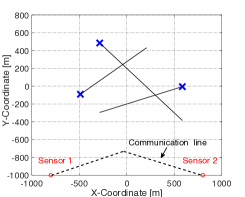
Refer to caption

(a)

Refer to caption

(b)

Figure 2: (a) The scenario of the distributed sensor network with two sensors tracking three objects. The initial positions of the objects are indicated by crosses. (b) The curves of OSPA errors of local filter, the standard GCI-MB fusion and the P-GCI-MB fusion.

VI-B Scenario 2

To examine the performance of the P-GCI-MB fusion in challenging scenarios, we consider a distributed sensor network with six sensors tracking forty objects in a [2000  2000]delimited-[]20002000[-2000\,\,2000] m ×\times [2000  2000]delimited-[]20002000[-2000\,\,2000] m surveillance region. The sketch map of this scenario is given in Fig. 3 (a), and the duration of tracking is T=200𝑇200T=200 s. Further, Fig. 3 (b) shows superposition of all observations acquired by Sensor 5 during the period of 1–200 s.
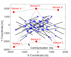
Refer to caption

(a)

Refer to caption

(b)

Figure 3: (a) The scenario of a distributed sensor network with three sensors tracking 50 objects, where the initial positions of objects are indicated by crosses. Each sensor can only exchange posteriors with its neighbor(s); (b) Superposition of all observations acquired by Sensor 5 during 1–200 s, where each blue dot denotes either the observation of an object or a clutter report.

In order to demonstrate both the computational efficiency and estimation accuracy of the proposed P-GCI-MB method, here we compare it with the GCI fusion with PHD filter (GCI-PHD) in [5] and the GCI fusion with CPHD filter (GCI-CPHD) in [7]. The PHD filter [10], CPHD filter [14] and cardinality balanced MB filter [15] are chosen as the local filter for GCI-PHD fusion, GCI-CPHD fusion and P-GCI-MB fusion, respectively. Since the objects appear at unknown positions and unknown time, the MB filters adopt the adaptive birth procedure introduced in [35], and the PHD/CPHD filters use the adaptive birth distribution introduced in [45].

The implementation parameters of different algorithms are chosen as follows. For the P-GCI-MB fusion, the maximum number of Bernoulli components is set to 100100100; the truncation threshold for Bernoulli components is γt=104subscript𝛾𝑡superscript104\gamma_{t}=10^{-4}; the maximum number, the pruning and merging thresholds of Gaussian components, and the GCI divergence threshold are set to be the same as Scenario 1. For the GCI-CPHD and GCI-PHD fusion, the maximum number of Gaussian components is set to 150150150; the pruning and merging thresholds for Gaussian components are the same as the P-GCI-MB fusion.

Regarding the sensor network topological structure, each sensor is linked with its neighbor(s) via the communication line as shown in Fig. 3 (a). Through the communication line, sensors can only exchange posteriors with their neighbor(s). Therefore, for example, sensor 5 performs fusion with five posteriors from sensors 1, 3, 4 and 6, and the local filter by sequentially applying the pairwise fusion four times.
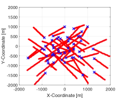
Refer to caption

(a)

Refer to caption

(b)

Figure 4: (a) Output of P-GCI-MB fusion for a single MC run, with object estimates indicated by red circles; (b) Tracking performance of P-GCI-MB, GCI-PHD and GCI-CPHD fusion algorithms at Sensor 5.

Refer to caption

(a)

Refer to caption

(b)

Refer to caption

(c)

Refer to caption

(d)

Figure 5: Cardinality statistics at Sensor 5: (a) P-GCI-MB fusion; (b) GCI-PHD fusion; (c) GCI-CPHD fusion; (d) execution times.

Fig. 4 (b) first shows the outputs of P-GCI-MB for a single MC run. It can be seen that P-GCI-MB performs accurately and consistently in the sense that it maintains locking on all objects and correctly estimates object positions for the entire scenario. Next, the OSPA errors for tracking results returned by the fusion algorithms performed at Sensor 5 are shown in Fig. 4 (b). The OSPA error curves clearly demonstrate the performance difference among the P-GCI-MB, GCI-CPHD and GCI-PHD fusions. Generally speaking, both P-GCI-MB and GCI-CPHD outperform GCI-PHD, with much lower OSPA errors. Moreover, at the times of object death including 30 s, 60 s, 65 s, 70 s, 120 s, etc., the OSPA errors of the P-GCI-MB fusion converge very fast, while the fusion performance of GCI-CPHD decreases a lot and hence a “peak” arises at its curve. After each transients, the performance of P-GCI-MB and GCI-CPHD are at the same level.

Figs. 5 (a) - (c) present the cardinality estimates and the corresponding standard deviations (Std.) returned by P-GCI-MB, GCI-CPHD and GCI-PHD at Sensor 5. It shows that the cardinality estimates given by both P-GCI-MB and GCI-CPHD are more accurate with less variations (higher level of confidence) than the GCI-PHD fusion. Further, when objects disappear, the convergence rate of cardinality estimation curve for the P-GCI-MB is faster than the GCI-CPHD.

Additionally, the comparison of the averaged execution time per time step among the P-GCI-MB, GCI-PHD and GCI-CPHD fusion methods are shown in Fig. 5 (d). It can be seen that the average execution time of P-GCI-MB fusion is less than GCI-CPHD and GCI-PHD over almost all time steps. Furthermore, the time gaps among P-GCI-MB, GCI-CPHD and GCI-PHD fusions become more distinct when there are more than ten objects appear in the scenario.

VII Conclusion

This paper investigates an efficient distributed fusion with multi-Bernoulli filters based on generalized Covariance Intersection. By discarding the inter-cluster hypotheses in the original fused posterior, the fused posterior is simplified to multiple independent fused ones with a smaller number of hypothetic objects, which leads to a significant computational reduction as well as an appealing parallel calculation. The characterization of the L1subscript𝐿1L_{1}-error for the approximation is also analysed. The efficiency of the proposed algorithm is verified via numerical results.

Appendix A Proof of Proposition 1

Proof.

Recall that π~ω(X)subscriptsuperscript~𝜋𝜔𝑋\widetilde{\pi}^{\prime}_{\omega}(X), which is the un-normalized GMB fused density after discarding all inter-cluster hypotheses, is computed by (31). For each hypothesis involved in π~ω(X)subscriptsuperscript~𝜋𝜔𝑋\widetilde{\pi}^{\prime}_{\omega}(X), i.e., (I1,θ)(𝕃1)×Θ𝔻subscript𝐼1𝜃subscript𝕃1Θ𝔻(I_{1},\theta)\in\mathcal{F}(\mathbb{L}_{1})\times\Theta-\mathbb{D}, we have θ()=θg()𝜃subscript𝜃𝑔\theta(\ell)=\theta_{g}(\ell) for each 𝕃1,gsubscript𝕃1𝑔\ell\in\mathbb{L}_{1,g}, g{g:𝒞gCI}𝑔conditional-set𝑔subscript𝒞𝑔subscript𝐶Ig\in\{g:\mathcal{C}_{g}\in C_{\text{I}}\}. Then, utilzing Definition 1, the space (𝕃1)×Θ𝔻subscript𝕃1Θ𝔻\mathcal{F}(\mathbb{L}_{1})\times\Theta-\mathbb{D} can be further represented as

(𝕃1)×Θ𝔻=g:𝒞gCI(𝕃1,g)×Θg.subscript𝕃1Θ𝔻subscript:𝑔subscript𝒞𝑔subscript𝐶Isubscript𝕃1𝑔subscriptΘ𝑔\mathcal{F}(\mathbb{L}_{1})\times\Theta-\mathbb{D}=\bigcup_{g:\mathcal{C}_{g}\in C_{\text{I}}}\mathcal{F}(\mathbb{L}_{1,g})\times\Theta_{g}. (75)

According to (5), the parameter Q1I1superscriptsubscript𝑄1subscript𝐼1Q_{1}^{I_{1}} in (14) can be further rewritten as

Q1I1=g:𝒞gCI𝕃1,g\(I1𝕃1,g)(1rs())I1𝕃1,grs()=g:𝒞gCIQ1,gI1𝕃1,g,superscriptsubscript𝑄1subscript𝐼1subscriptproduct:𝑔subscript𝒞𝑔subscript𝐶Isubscriptproduct\subscript𝕃1𝑔subscript𝐼1subscript𝕃1𝑔1superscriptsubscript𝑟𝑠subscriptproductsuperscriptsubscript𝐼1subscript𝕃1𝑔superscriptsubscript𝑟𝑠subscriptproduct:𝑔subscript𝒞𝑔subscript𝐶Isuperscriptsubscript𝑄1𝑔subscript𝐼1subscript𝕃1𝑔\begin{split}Q_{1}^{I_{1}}=&\prod_{g:\mathcal{C}_{g}\in C_{\text{I}}}\prod_{\ell\in\mathbb{L}_{1,g}\backslash(I_{1}\cap\mathbb{L}_{1,g})}(1-r_{s}^{(\ell)})\prod_{\ell^{\prime}\in I_{1}\cap\mathbb{L}_{1,g}}r_{s}^{(\ell)}\\ =&\prod_{g:\mathcal{C}_{g}\in C_{\text{I}}}Q_{1,g}^{I_{1}\cap\mathbb{L}_{1,g}},\end{split} (76)

where Q1,gI1𝕃1,gsuperscriptsubscript𝑄1𝑔subscript𝐼1subscript𝕃1𝑔Q_{1,g}^{I_{1}\cap\mathbb{L}_{1,g}} is the corresponding parameter of the g𝑔gth cluster at sensor 1; while, similarly, Q2θ(I1)superscriptsubscript𝑄2𝜃subscript𝐼1Q_{2}^{\theta(I_{1})} in (14) can be rewritten as

Q2θ(I1)=g:𝒞gCIQ2,gθ(I1)𝕃2,g=g:𝒞gCIQ2,gθ(I1𝕃1,g).superscriptsubscript𝑄2𝜃subscript𝐼1subscriptproduct:𝑔subscript𝒞𝑔subscript𝐶Isuperscriptsubscript𝑄2𝑔𝜃subscript𝐼1subscript𝕃2𝑔subscriptproduct:𝑔subscript𝒞𝑔subscript𝐶Isuperscriptsubscript𝑄2𝑔𝜃subscript𝐼1subscript𝕃1𝑔\displaystyle Q_{2}^{\theta(I_{1})}=\prod_{g:\mathcal{C}_{g}\in C_{\text{I}}}Q_{2,g}^{\theta(I_{1})\cap\mathbb{L}_{2,g}}=\prod_{g:\mathcal{C}_{g}\in C_{\text{I}}}Q_{2,g}^{\theta(I_{1}\cap\mathbb{L}_{1,g})}. (77)

Since we have θ()=θg()𝜃subscript𝜃𝑔\theta(\ell)=\theta_{g}(\ell) for each I1𝕃1,gsubscript𝐼1subscript𝕃1𝑔\ell\in I_{1}\cap\mathbb{L}_{1,g}, hence,

Q2θ(I1)=g:𝒞gCIQ2,gθg(I1𝕃1,g).superscriptsubscript𝑄2𝜃subscript𝐼1subscriptproduct:𝑔subscript𝒞𝑔subscript𝐶Isuperscriptsubscript𝑄2𝑔subscript𝜃𝑔subscript𝐼1subscript𝕃1𝑔Q_{2}^{\theta(I_{1})}=\prod_{g:\mathcal{C}_{g}\in C_{\text{I}}}Q_{2,g}^{\theta_{g}(I_{1}\cap\mathbb{L}_{1,g})}. (78)

Similarly, the following holds:

p(,θ)(x)=p(,θg)(x),I1𝕃1,g,g{g:𝒞gCI},formulae-sequencesuperscript𝑝𝜃𝑥superscript𝑝subscript𝜃𝑔𝑥formulae-sequencesubscript𝐼1subscript𝕃1𝑔𝑔conditional-set𝑔subscript𝒞𝑔subscript𝐶Ip^{(\ell,\theta)}(x)=p^{(\ell,\theta_{g})}(x),\ell\in I_{1}\cap\mathbb{L}_{1,g},g\in\{g:\mathcal{C}_{g}\in C_{\text{I}}\}, (79)

and hence the term, I1Zω(,θ)subscriptproductsubscript𝐼1superscriptsubscript𝑍𝜔𝜃{\prod}_{\ell\in I_{1}}Z_{\omega}^{(\ell,\theta)} in (14) can be factorized as

I1Zω(,θ)=g:𝒞gCII1𝕃1,gZω,g(,θg),subscriptproductsubscript𝐼1superscriptsubscript𝑍𝜔𝜃subscriptproduct:𝑔subscript𝒞𝑔subscript𝐶Isubscriptproductsubscript𝐼1subscript𝕃1𝑔superscriptsubscript𝑍𝜔𝑔subscript𝜃𝑔\prod_{\ell\in I_{1}}Z_{\omega}^{(\ell,\theta)}=\prod_{g:\mathcal{C}_{g}\in C_{\text{I}}}\prod_{\ell\in I_{1}\cap\mathbb{L}_{1,g}}Z_{\omega,g}^{(\ell,\theta_{g})}, (80)

where Zω,g(,θg)superscriptsubscript𝑍𝜔𝑔subscript𝜃𝑔Z_{\omega,g}^{(\ell,\theta_{g})} is given in (41)41(\ref{Z_w-g}).

As a result, based on (76), (78) and (80), the un-normalized weight in (14) yields

w~ω(I1,θ)=g:𝒞gCIw~ω(I1𝕃1,g,θg),superscriptsubscript~𝑤𝜔subscript𝐼1𝜃subscriptproduct:𝑔subscript𝒞𝑔subscript𝐶Isuperscriptsubscript~𝑤𝜔subscript𝐼1subscript𝕃1𝑔subscript𝜃𝑔\widetilde{w}_{\omega}^{(I_{1},\theta)}=\prod_{g:\mathcal{C}_{g}\in C_{\text{I}}}\widetilde{w}_{\omega}^{(I_{1}\cap\mathbb{L}_{1,g},\theta_{g})}, (81)

where w~ω(I1𝕃1,g,θg)superscriptsubscript~𝑤𝜔subscript𝐼1subscript𝕃1𝑔subscript𝜃𝑔\widetilde{w}_{\omega}^{(I_{1}\cap\mathbb{L}_{1,g},\theta_{g})} is given in (40). Then, using (75), (79) and (81), (31) can be further simplified as (83), where π~ω,g()subscript~𝜋𝜔𝑔\widetilde{\pi}_{\omega,g}(\cdot) is the un-normalized fused density of the g𝑔gth cluster,

π~ω,g({x1,,xn})=σ(I1,g,θ)n(𝕃1,g)×Θg(I1,g)w~ω(I1,g,θg)i=1npω([I1,g]v(i),θg)(xσ(i)).subscript~𝜋𝜔𝑔subscript𝑥1subscript𝑥𝑛subscript𝜎subscriptsubscript𝐼1𝑔𝜃subscript𝑛subscript𝕃1𝑔subscriptΘ𝑔subscript𝐼1𝑔superscriptsubscript~𝑤𝜔subscript𝐼1𝑔subscript𝜃𝑔superscriptsubscriptproduct𝑖1𝑛superscriptsubscript𝑝𝜔superscriptdelimited-[]subscript𝐼1𝑔𝑣𝑖subscript𝜃𝑔subscript𝑥𝜎𝑖\begin{split}\!\!\!\widetilde{\pi}_{\omega,g}(\{x_{1},\!\cdots\!,x_{n}\})\!=\!&\sum_{\sigma}\sum_{(I_{1,g},\theta)\in\mathcal{F}_{n}\!(\mathbb{L}_{1,g}\!)\!\times\!\Theta_{g}({I_{1,g}})}\!\!\!\widetilde{w}_{\omega}^{(I_{1,g},\theta_{g})}\\ &\cdot{\prod}_{i=1}^{n}p_{\omega}^{([I_{1,g}]^{v}\!(i),\theta_{g})}\!(x_{\sigma(i)}).\end{split} (82)
π~ω({x1,,xn})=σ(I1,θ)n(𝕃1)×ΘI1𝔻w~ω(I1,θ)i=1npω(𝐈1v(i),θ)(xσ(i))=g:𝒞gCI{xg1,,xgng}={x1,,xn}σg:{1,,ng}{1,,ng},g:𝒞gCI(I1,g,θg)ng(𝕃1,g×Θg),g:𝒞gCIg:𝒞gCIw~ω(I1,g,θg)j=1ngpω([I1,g]v(j),θg)(xσ(gj))=g:𝒞gCI{xg1,,xgng}={x1,,xn}g:𝒞gCIσg:{1,,ng}{1,,ng}(I1,g,θg)ng(𝕃1,g)×Θgw~ω,g(I1,g,θg)j=1ngpω,g([I1,g]v(j),θg)(xgσ(j))=g:𝒞gCIXg={x1,,xn}g=1N𝒞π~ω,g(Xg)subscriptsuperscript~𝜋𝜔subscript𝑥1subscript𝑥𝑛subscript𝜎subscriptsubscript𝐼1𝜃subscript𝑛subscript𝕃1subscriptΘsubscript𝐼1𝔻superscriptsubscript~𝑤𝜔subscript𝐼1𝜃superscriptsubscriptproduct𝑖1𝑛superscriptsubscript𝑝𝜔superscriptsubscript𝐈1𝑣𝑖𝜃subscript𝑥𝜎𝑖subscriptsubscriptsymmetric-difference:𝑔subscript𝒞𝑔subscript𝐶Isubscript𝑥subscript𝑔1subscript𝑥subscript𝑔subscript𝑛𝑔subscript𝑥1subscript𝑥𝑛subscript:subscript𝜎𝑔1subscript𝑛𝑔1subscript𝑛𝑔:𝑔subscript𝒞𝑔subscript𝐶Isubscriptsubscript𝐼1𝑔subscript𝜃𝑔subscriptsubscript𝑛𝑔subscript𝕃1𝑔subscriptΘ𝑔:𝑔subscript𝒞𝑔subscript𝐶Isubscriptproduct:𝑔subscript𝒞𝑔subscript𝐶Isuperscriptsubscript~𝑤𝜔subscript𝐼1𝑔subscript𝜃𝑔superscriptsubscriptproduct𝑗1subscript𝑛𝑔superscriptsubscript𝑝𝜔superscriptdelimited-[]subscript𝐼1𝑔𝑣𝑗subscript𝜃𝑔subscript𝑥𝜎subscript𝑔𝑗subscriptsubscriptsymmetric-difference:𝑔subscript𝒞𝑔subscript𝐶Isubscript𝑥subscript𝑔1subscript𝑥subscript𝑔subscript𝑛𝑔subscript𝑥1subscript𝑥𝑛subscriptproduct:𝑔subscript𝒞𝑔subscript𝐶Isubscript:subscript𝜎𝑔1subscript𝑛𝑔1subscript𝑛𝑔subscriptsubscript𝐼1𝑔subscript𝜃𝑔subscriptsubscript𝑛𝑔subscript𝕃1𝑔subscriptΘ𝑔superscriptsubscript~𝑤𝜔𝑔subscript𝐼1𝑔subscript𝜃𝑔superscriptsubscriptproduct𝑗1subscript𝑛𝑔superscriptsubscript𝑝𝜔𝑔superscriptdelimited-[]subscript𝐼1𝑔𝑣𝑗subscript𝜃𝑔subscript𝑥subscript𝑔𝜎𝑗subscriptsubscriptsymmetric-difference:𝑔subscript𝒞𝑔subscript𝐶Isubscript𝑋𝑔subscript𝑥1subscript𝑥𝑛superscriptsubscriptproduct𝑔1subscript𝑁𝒞subscript~𝜋𝜔𝑔subscript𝑋𝑔\begin{split}&\widetilde{\pi}^{\prime}_{\omega}(\!\left\{x_{1},\!\cdots\!,x_{n}\right\})=\sum_{\sigma}\sum_{(I_{1},\theta)\in\mathcal{F}_{n}(\mathbb{L}_{1})\times\Theta_{I_{1}}-\mathbb{D}}\widetilde{w}_{\omega}^{(I_{1},\theta)}{\prod}_{i=1}^{n}p_{\omega}^{({\bf I}_{1}^{v}(i),\theta)}(x_{\sigma(i)}\!)\\ =&\sum_{\biguplus_{g:\mathcal{C}_{g}\in C_{\text{I}}}\{x_{g_{1}},\cdots,x_{g_{n_{g}}}\}=\{x_{1},\cdots,x_{n}\}}\sum_{\begin{subarray}{c}\sigma_{g}:\{1,\cdots,n_{g}\}\rightarrow\{1,\cdots,n_{g}\},\\ g:\mathcal{C}_{g}\in C_{\text{I}}\end{subarray}}\sum_{\begin{subarray}{c}(I_{1,g},\theta_{g})\in\mathcal{F}_{n_{g}}(\mathbb{L}_{1,g}\times\Theta_{g}),\\ g:\mathcal{C}_{g}\in C_{\text{I}}\end{subarray}}\prod_{g:\mathcal{C}_{g}\in C_{\text{I}}}\widetilde{w}_{\omega}^{(I_{1,g},\theta_{g})}\prod_{j=1}^{n_{g}}p_{\omega}^{([I_{1,g}]^{v}(j),\theta_{g})}(x_{\sigma(g_{j})})\\ =&\sum_{\biguplus_{g:\mathcal{C}_{g}\in C_{\text{I}}}\{x_{g_{1}},\cdots,x_{g_{n_{g}}}\}=\{x_{1},\cdots,x_{n}\}}\prod_{g:\mathcal{C}_{g}\in C_{\text{I}}}\sum_{\sigma_{g}:\{1,\cdots,n_{g}\}\rightarrow\{1,\cdots,n_{g}\}}\sum_{\begin{subarray}{c}(I_{1,g},\theta_{g})\end{subarray}\in\mathcal{F}_{n_{g}}(\mathbb{L}_{1,g})\times\Theta_{g}}\widetilde{w}_{\omega,g}^{(I_{1,g},\theta_{g})}\prod_{j=1}^{n_{g}}p_{\omega,g}^{([I_{1,g}]^{v}(j),\theta_{g})}(x_{g_{\sigma(j)}})\\ =&\sum_{\biguplus_{g:\mathcal{C}_{g}\in C_{\text{I}}}X_{g}=\{x_{1},\cdots,x_{n}\}}\prod_{g=1}^{N_{\mathcal{C}}}\widetilde{\pi}_{\omega,g}(X_{g})\end{split} (83)


Further, based on (83), the normalized constant ηωsubscript𝜂𝜔\eta_{\omega} can be computed by:

ηω=I1(𝕃1)θΘI1w~ω(I1,θ)=g:𝒞gCII1,g(𝕃1,g)θgΘg(I1)w~ω(I1,θ)=g:𝒞gCIηω,g.subscript𝜂𝜔subscriptsubscript𝐼1subscript𝕃1subscript𝜃subscriptΘsubscript𝐼1superscriptsubscript~𝑤𝜔subscript𝐼1𝜃subscriptproduct:𝑔subscript𝒞𝑔subscript𝐶Isubscriptsubscript𝐼1𝑔subscript𝕃1𝑔subscriptsubscript𝜃𝑔subscriptΘ𝑔subscript𝐼1superscriptsubscript~𝑤𝜔subscript𝐼1𝜃subscriptproduct:𝑔subscript𝒞𝑔subscript𝐶Isubscript𝜂𝜔𝑔\begin{split}\eta_{\omega}&=\sum_{I_{1}\in\mathcal{F}(\mathbb{L}_{1})}\sum_{\theta\in\Theta_{I_{1}}}\widetilde{w}_{\omega}^{(I_{1},\theta)}\,\,\,\,\,\\ &=\prod_{g:\mathcal{C}_{g}\in C_{\text{I}}}{\sum}_{I_{1,g}\in\mathcal{F}(\mathbb{L}_{1,g})}{\sum}_{\theta_{g}\in\Theta_{g}(I_{1})}\widetilde{w}_{\omega}^{(I_{1},\theta)}\\ &=\prod_{g:\mathcal{C}_{g}\in C_{\text{I}}}\eta_{\omega,g}.\end{split} (84)

Hence, substituting (83) and (84) into (33), we have

πω(X)=g:𝒞gCIXg=Xg:𝒞gCIπ~ω,g(Xg)/ηω,g=g:𝒞gCIXg=Xg:𝒞gCIπω,g(Xg).subscriptsuperscript𝜋𝜔𝑋subscriptsubscriptsymmetric-difference:𝑔subscript𝒞𝑔subscript𝐶Isubscript𝑋𝑔𝑋subscriptproduct:𝑔subscript𝒞𝑔subscript𝐶Isubscript~𝜋𝜔𝑔subscript𝑋𝑔subscript𝜂𝜔𝑔subscriptsubscriptsymmetric-difference:𝑔subscript𝒞𝑔subscript𝐶Isubscript𝑋𝑔𝑋subscriptproduct:𝑔subscript𝒞𝑔subscript𝐶Isubscript𝜋𝜔𝑔subscript𝑋𝑔\begin{split}&\pi^{\prime}_{\omega}(X)\\ =&\sum_{\biguplus_{g:\mathcal{C}_{g}\in C_{\text{I}}}X_{g}=X}\prod_{g:\mathcal{C}_{g}\in C_{\text{I}}}\!\widetilde{\pi}_{\omega,g}(X_{g})/\eta_{\omega,g}\\ =&\sum_{\biguplus_{g:\mathcal{C}_{g}\in C_{\text{I}}}X_{g}=X}\prod_{g:\mathcal{C}_{g}\in C_{\text{I}}}\pi_{\omega,g}(X_{g}).\end{split} (85)

Hence, the Proposition holds. ∎

Appendix B Proof of Proposition 2

Proof.

Based on (75), we can further obtain that

NH=|(𝕃)×Θ𝔻|=g:𝒞gCI|(𝕃1,g)×Θg|.superscriptsubscript𝑁𝐻𝕃Θ𝔻subscriptproduct:𝑔subscript𝒞𝑔subscript𝐶Isubscript𝕃1𝑔subscriptΘ𝑔N_{H}^{\prime}=|\mathcal{F}(\mathbb{L})\times\Theta-\mathbb{D}|=\prod_{g:\mathcal{C}_{g}\in C_{\text{I}}}|\mathcal{F}(\mathbb{L}_{1,g})\times\Theta_{g}|. (86)

Consider a function

ϕ(a1,,aN)=i=1Naii=1Nai,italic-ϕsubscript𝑎1subscript𝑎𝑁superscriptsubscriptproduct𝑖1𝑁subscript𝑎𝑖superscriptsubscript𝑖1𝑁subscript𝑎𝑖\phi(a_{1},\cdots,a_{N})=\prod_{i=1}^{N}a_{i}-\sum_{i=1}^{N}a_{i}, (87)

with N2𝑁2{N}\geq 2.

It can be easily checked that if a1==aN=2subscript𝑎1subscript𝑎𝑁2a_{1}=\cdots=a_{N}=2, the following holds:

ϕ(a1,,aN)0italic-ϕsubscript𝑎1subscript𝑎𝑁0\phi(a_{1},\cdots,a_{N})\geq 0 (88)

where the equality holds up if and only if N=2𝑁2{N}=2.

The partial derivative of ϕ(a1,,aN)italic-ϕsubscript𝑎1subscript𝑎𝑁\phi(a_{1},\cdots,a_{N}) with respective to aisubscript𝑎𝑖a_{i} is computed by

dϕdai=ai(i{1,,N}\{i}ai1),i=1,,Nformulae-sequence𝑑italic-ϕ𝑑subscript𝑎𝑖subscript𝑎𝑖subscriptproductsuperscript𝑖\1𝑁𝑖subscript𝑎superscript𝑖1𝑖1𝑁\frac{d\,\phi}{d\,a_{i}}=a_{i}(\prod_{i^{\prime}\in\{1,\cdots,{N}\}\backslash\{i\}}a_{i^{\prime}}-1),i=1,\cdots,N (89)

Hence, for ai>2,i=1,,Nformulae-sequencesubscript𝑎𝑖2𝑖1𝑁a_{i}>2,i=1,\cdots,N, we have

dϕdai>0,𝑑italic-ϕ𝑑subscript𝑎𝑖0\displaystyle\frac{d\,\phi}{d\,a_{i}}>0, (90)

and thus the following holds:

ϕ(a1,,aN)>0.italic-ϕsubscript𝑎1subscript𝑎𝑁0\phi(a_{1},\cdots,a_{N})>0. (91)

Define each item aisubscript𝑎𝑖a_{i} in (87) as |(𝕃1,g)×Θg|absentsubscript𝕃1𝑔subscriptΘ𝑔\triangleq|\mathcal{F}(\mathbb{L}_{1,g})\times\Theta_{g}| for each g:𝒞gI:𝑔subscript𝒞𝑔subscriptIg:\mathcal{C}_{g}\in\mathbb{C}_{\text{I}}. It can be easily checked that |(𝕃1,g)×Θg|2subscript𝕃1𝑔subscriptΘ𝑔2|\mathcal{F}(\mathbb{L}_{1,g})\times\Theta_{g}|\geq 2 if 𝕃1,g1subscript𝕃1𝑔1\mathbb{L}_{1,g}\geq 1, where the equality holds if and only if 𝕃1,g=1subscript𝕃1𝑔1\mathbb{L}_{1,g}=1 and 𝕃2,g=1subscript𝕃2𝑔1\mathbb{L}_{2,g}=1. Hence, we have

g:𝒞gI|(𝕃1,g)×Θg|g:𝒞gI|(𝕃1,g)×Θg|0subscriptproduct:𝑔subscript𝒞𝑔subscriptIsubscript𝕃1𝑔subscriptΘ𝑔subscript:𝑔subscript𝒞𝑔subscriptIsubscript𝕃1𝑔subscriptΘ𝑔0\prod_{g:\mathcal{C}_{g}\in\mathbb{C}_{\text{I}}}|\mathcal{F}(\mathbb{L}_{1,g})\times\Theta_{g}|-\sum_{g:\mathcal{C}_{g}\in\mathbb{C}_{\text{I}}}|\mathcal{F}(\mathbb{L}_{1,g})\times\Theta_{g}|\geq 0 (92)

if 𝕃1,g1,g:𝒞gI:subscript𝕃1𝑔1𝑔subscript𝒞𝑔subscriptI\mathbb{L}_{1,g}\geq 1,g:\mathcal{C}_{g}\in\mathbb{C}_{\text{I}}, where the equality holds if and only if 𝕃1,g=1subscript𝕃1𝑔1\mathbb{L}_{1,g}=1, 𝕃2,g=1subscript𝕃2𝑔1\mathbb{L}_{2,g}=1 and N𝒞I=2subscript𝑁subscript𝒞I2N_{\mathcal{C}_{\text{I}}}=2. ∎

Appendix C Proof of Proposition 3

Proof.

Based on the definition of L1subscript𝐿1L_{1}-norm, we have,

πω()πω()1|σ(I1,θ)𝔻(w~ω(I1,θ)ηωw~ω(I1,θ)ηω)i=1npω([I1]v(i),θ)(xσ(i))|δXsubscriptdelimited-∥∥subscript𝜋𝜔subscriptsuperscript𝜋𝜔1subscript𝜎subscriptsubscript𝐼1𝜃𝔻superscriptsubscript~𝑤𝜔subscript𝐼1𝜃subscript𝜂𝜔superscriptsubscript~𝑤𝜔subscript𝐼1𝜃subscriptsuperscript𝜂𝜔superscriptsubscriptproduct𝑖1𝑛superscriptsubscript𝑝𝜔superscriptdelimited-[]subscript𝐼1𝑣𝑖𝜃subscript𝑥𝜎𝑖𝛿𝑋\begin{split}&\,\,\,\,\,\,\,\left\|\pi_{\omega}(\cdot)-\pi^{\prime}_{\omega}(\cdot)\right\|_{1}\\ &\leqslant\int\left|\sum_{\sigma}\!\sum_{(I_{1},\theta)\in\mathbb{H}-\mathbb{D}}\!\left(\!\frac{\widetilde{w}_{\omega}^{(I_{1},\theta)}}{\eta_{\omega}}\!-\!\frac{\widetilde{w}_{\omega}^{(I_{1},\theta)}}{\eta^{\prime}_{\omega}}\!\right)\!\prod_{i=1}^{n}p_{\omega}^{([I_{1}]^{v}(i),\theta)}(x_{\sigma(i)})\right|\delta X\\ \end{split}
+|σ(I1,θ)𝔻w~ω(I1,θ)ηωi=1npω([I1]v(i),θ)(xσ(i))|δX=(I1,θ)𝔻|w~ω(I1,θ)ηωw~ω(I1,θ)ηω|+(I1,θ)𝔻w~ω(I1,θ)ηω=1ηωηω+ηωηωηω=2(ηωηω)ηω=2(I,θ)𝔻w~ω(I1,θ)/ηω=2(I1,θ)𝔻(Q1I1)ω1(Q2θ(I1))ω2exp(I1d(,θ()))/ηωsubscript𝜎subscriptsubscript𝐼1𝜃𝔻superscriptsubscript~𝑤𝜔subscript𝐼1𝜃subscriptsuperscript𝜂𝜔superscriptsubscriptproduct𝑖1𝑛superscriptsubscript𝑝𝜔superscriptdelimited-[]subscript𝐼1𝑣𝑖𝜃subscript𝑥𝜎𝑖𝛿𝑋subscriptsubscript𝐼1𝜃𝔻superscriptsubscript~𝑤𝜔subscript𝐼1𝜃subscript𝜂𝜔superscriptsubscript~𝑤𝜔subscript𝐼1𝜃subscriptsuperscript𝜂𝜔subscriptsubscript𝐼1𝜃𝔻superscriptsubscript~𝑤𝜔subscript𝐼1𝜃subscriptsuperscript𝜂𝜔1subscriptsuperscript𝜂𝜔subscript𝜂𝜔subscript𝜂𝜔subscriptsuperscript𝜂𝜔subscriptsuperscript𝜂𝜔2subscript𝜂𝜔subscriptsuperscript𝜂𝜔subscript𝜂𝜔2subscript𝐼𝜃𝔻superscriptsubscript~𝑤𝜔subscript𝐼1𝜃subscript𝜂𝜔2subscriptsubscript𝐼1𝜃𝔻superscriptsuperscriptsubscript𝑄1subscript𝐼1subscript𝜔1superscriptsuperscriptsubscript𝑄2𝜃subscript𝐼1subscript𝜔2subscriptsubscript𝐼1𝑑𝜃subscript𝜂𝜔\begin{split}&\,\,\,\,\,\,\,\,\,+\int\left|\sum_{\sigma}\sum_{(I_{1},\theta)\in\mathbb{D}}\frac{\widetilde{w}_{\omega}^{(I_{1},\theta)}}{\eta^{\prime}_{\omega}}\,\prod_{i=1}^{n}p_{\omega}^{([I_{1}]^{v}(i),\theta)}(x_{\sigma(i)})\right|\delta X\\ &=\sum_{(I_{1},\theta)\in\mathbb{H}-\mathbb{D}}\left|\frac{\widetilde{w}_{\omega}^{(I_{1},\theta)}}{\eta_{\omega}}-\frac{\widetilde{w}_{\omega}^{(I_{1},\theta)}}{\eta^{\prime}_{\omega}}\right|+\sum_{(I_{1},\theta)\in\mathbb{D}}\frac{\widetilde{w}_{\omega}^{(I_{1},\theta)}}{\eta^{\prime}_{\omega}}\\ &=1-\frac{\eta^{\prime}_{\omega}}{\eta_{\omega}}+\frac{\eta_{\omega}-\eta^{\prime}_{\omega}}{\eta^{\prime}_{\omega}}\\ &=2\frac{(\eta_{\omega}-\eta^{\prime}_{\omega})}{\eta_{\omega}}=2\sum_{(I,\theta)\in\mathbb{D}}\widetilde{w}_{\omega}^{(I_{1},\theta)}\big{/}\eta_{\omega}\\ &=2\sum_{(I_{1},\theta)\in\mathbb{D}}\!\!\left(Q_{1}^{I_{1}}\right)^{\omega_{1}}\!\!\left(Q_{2}^{\theta(I_{1})}\right)^{\omega_{2}}\!\!\exp(-\!\sum_{\ell\in I_{1}}d(\ell,\theta(\ell)))\big{/}\eta_{\omega}\end{split} (93)

Hence, the Proposition holds. ∎

Appendix D Lemma 1 and Proof of Proposition 4

D-A Lemma 1 and a proof

Lemma 1.

Suppose that (𝕃1a,𝕃2a)superscriptsubscript𝕃1𝑎superscriptsubscript𝕃2𝑎(\mathbb{L}_{1}^{a},\mathbb{L}_{2}^{a}) and (𝕃1b,𝕃2b)superscriptsubscript𝕃1𝑏superscriptsubscript𝕃2𝑏(\mathbb{L}_{1}^{b},\mathbb{L}_{2}^{b}) are two mutually isolated clusters of (𝕃1,𝕃2)subscript𝕃1subscript𝕃2(\mathbb{L}_{1},\mathbb{L}_{2}). There is no path between any label a𝕃1asubscript𝑎superscriptsubscript𝕃1𝑎\ell_{a}\in\mathbb{L}_{1}^{a} and any label b𝕃1bsubscript𝑏superscriptsubscript𝕃1𝑏\ell_{b}\in\mathbb{L}_{1}^{b} in the undirected graph G(V,E)𝐺𝑉𝐸G(V,E) constructed by (𝕃1,𝕃2)subscript𝕃1subscript𝕃2(\mathbb{L}_{1},\mathbb{L}_{2}).

Proof.

This proposition is proved by reductio. Suppose that there exists a path between a𝕃1asubscript𝑎superscriptsubscript𝕃1𝑎\ell_{a}\in\mathbb{L}_{1}^{a} and b𝕃1bsubscript𝑏superscriptsubscript𝕃1𝑏\ell_{b}\in\mathbb{L}_{1}^{b}, denoted by an alternating sequence of vertices and edges, a,ea,1,e1,,K,eK,bsubscript𝑎subscript𝑒𝑎subscript1subscript𝑒1subscript𝐾subscript𝑒𝐾subscript𝑏\ell_{a},e_{a},\ell_{1},e_{1},\cdots,\ell_{K},e_{K},\ell_{b}. Three cases which exhaust all possible paths are discussed as follow.

  • All non-end vertices 1,,Ksubscript1subscript𝐾\ell_{1},\cdots,\ell_{K} belong to 𝕃1asuperscriptsubscript𝕃1𝑎\mathbb{L}_{1}^{a}. Based on the definition of path, eK=(K,b)subscript𝑒𝐾subscript𝐾subscript𝑏e_{K}=(\ell_{K},\ell_{b}) is an edge. That is to say, Ksubscript𝐾\ell_{K} has common associated hypothetic objects from sensor 2 with hypothetic object bsubscript𝑏\ell_{b}. Thus, there is a hypothetic object 𝕃2bsuperscriptsuperscriptsubscript𝕃2𝑏\ell^{\prime}\in\mathbb{L}_{2}^{b} such that,

    d(K,)γ,𝑑subscript𝐾superscript𝛾d(\ell_{K},\ell^{\prime})\leq\gamma, (94)

    or there is a hypothetic object 𝕃2asuperscriptsuperscriptsubscript𝕃2𝑎\ell^{\prime}\in\mathbb{L}_{2}^{a} such that

    d(b,)γ𝑑subscript𝑏superscript𝛾d(\ell_{b},\ell^{\prime})\leq\gamma (95)
  • All non-end vertices 1,,Ksubscript1subscript𝐾\ell_{1},\cdots,\ell_{K} belong to 𝕃1bsuperscriptsubscript𝕃1𝑏\mathbb{L}_{1}^{b}. Similarly, ea=(a,1)subscript𝑒𝑎subscript𝑎subscript1e_{a}=(\ell_{a},\ell_{1}) is an edge, and thus there is a hypothetic object 𝕃2bsuperscriptsuperscriptsubscript𝕃2𝑏\ell^{\prime}\in\mathbb{L}_{2}^{b} such that

    d(a,)γ,𝑑subscript𝑎superscript𝛾d(\ell_{a},\ell^{\prime})\leq\gamma, (96)

    or or there is a hypothetic object 𝕃2asuperscriptsuperscriptsubscript𝕃2𝑎\ell^{\prime}\in\mathbb{L}_{2}^{a} such that

    d(1,)γ.𝑑subscript1superscript𝛾d(\ell_{1},\ell^{\prime})\leq\gamma. (97)
  • A part of non-end vertices 1,,Ksubscript1subscript𝐾\ell_{1},\cdots,\ell_{K} belong to 𝕃1asuperscriptsubscript𝕃1𝑎\mathbb{L}_{1}^{a}, while the other part K0+1,,Ksubscriptsubscript𝐾01subscript𝐾\ell_{K_{0}+1},\cdots,\ell_{K} belong to 𝕃1bsuperscriptsubscript𝕃1𝑏\mathbb{L}_{1}^{b}. Similarly, (K0,K0+1)subscriptsubscript𝐾0subscriptsubscript𝐾01(\ell_{K_{0}},\ell_{{K_{0}}+1}) is an edge. and thus there is a hypothetic object 𝕃2bsuperscriptsuperscriptsubscript𝕃2𝑏\ell^{\prime}\in\mathbb{L}_{2}^{b} such that

    d(K0,)γ,𝑑subscriptsubscript𝐾0superscript𝛾d(\ell_{K_{0}},\ell^{\prime})\leq\gamma, (98)

    or there is a hypothetic object 𝕃2asuperscriptsuperscriptsubscript𝕃2𝑎\ell^{\prime}\in\mathbb{L}_{2}^{a} such that

    d(K0+1,)γ.𝑑subscriptsubscript𝐾01superscript𝛾d(\ell_{K_{0}+1},\ell^{\prime})\leq\gamma. (99)

To summary, all the aforementioned cases are inconsistent with that (𝕃1a,𝕃2a)superscriptsubscript𝕃1𝑎superscriptsubscript𝕃2𝑎(\mathbb{L}_{1}^{a},\mathbb{L}_{2}^{a}) and (𝕃1b,𝕃2b)superscriptsubscript𝕃1𝑏superscriptsubscript𝕃2𝑏(\mathbb{L}_{1}^{b},\mathbb{L}_{2}^{b}) are isolated clusters. Consequently, there does not exist a path between asubscript𝑎\ell_{a} and bsubscript𝑏\ell_{b}, and the proposition holds. ∎

D-B A Proof of Proposition 4

Proof.

Firstly, we focus on proving that C𝐶C is an isolated clustering. As presented in Section IV-C 2), the union CICIIsubscript𝐶Isubscript𝐶IIC_{\text{I}}\cup C_{\text{II}} in the finalized clustering C𝐶C of (56) is obtained through seeking the connected components of the constructed undirected graph G(V,E)𝐺𝑉𝐸G(V,E). Recall the structure of the undirected graph, each vertex \ell represents a hypothetic object in 𝕃1subscript𝕃1\mathbb{L}_{1}, and the edge means that two hypothetic objects of sensor 1 have common associated hypothetic objects from sensor 2.

Based on the definition of the connected component, for any g1g2{g:𝒞gCICII}subscript𝑔1subscript𝑔2conditional-set𝑔subscript𝒞𝑔subscript𝐶Isubscript𝐶IIg_{1}\neq g_{2}\in\{g:\mathcal{C}_{g}\in C_{\text{I}}\cup C_{\text{II}}\}, any vertex in Vg1subscript𝑉subscript𝑔1V_{g_{1}} is not connected with any vertex in Vg2subscript𝑉subscript𝑔2V_{g_{2}}, and thus cannot be paired to be an edge. Hence, any hypothetic object 1𝕃1,g1(𝕃1,g1=Vg1)\ell_{1}\in\mathbb{L}_{1,_{g_{1}}}(\mathbb{L}_{1,{g_{1}}}=V_{g_{1}}) and any hypothetic object 2𝕃1,g2(𝕃1,g2=Vg2)subscript2subscript𝕃1subscript𝑔2subscript𝕃1subscript𝑔2subscript𝑉subscript𝑔2\ell_{2}\in\mathbb{L}_{1,g_{2}}(\mathbb{L}_{1,g_{2}}=V_{g_{2}}) have no common associated hypothetic objects from sensor 2. That is to say that for any two different clusters 𝒞g1subscript𝒞subscript𝑔1\mathcal{C}_{g_{1}} and 𝒞g2subscript𝒞subscript𝑔2\mathcal{C}_{g_{2}} of CICIIsubscript𝐶Isubscript𝐶IIC_{\text{I}}\cup C_{\text{II}}, the following holds:

𝕃2,g1𝕃2,g2=.subscript𝕃2subscript𝑔1subscript𝕃2subscript𝑔2\mathbb{L}_{2,g_{1}}\cap\mathbb{L}_{2,g_{2}}=\emptyset. (100)

In addition, for any cluster 𝒞g3CIIIsubscript𝒞subscript𝑔3subscript𝐶III\mathcal{C}_{g_{3}}\in C_{\text{III}} where CIIIsubscript𝐶IIIC_{\text{III}} is given in (53), we have 𝕃1,g3subscript𝕃1subscript𝑔3\mathbb{L}_{1,g_{3}} is an empty set and 𝕃2,g3𝕃2\(𝕃1Ψ2())subscript𝕃2subscript𝑔3\subscript𝕃2subscriptsubscript𝕃1superscriptsubscriptΨ2\mathbb{L}_{2,g_{3}}\subseteq\mathbb{L}_{2}\backslash(\cup_{\ell\in\mathbb{L}_{1}}\Psi_{2}^{(\ell)}). Then, based on (50) and (55), we have

𝕃2,g3(g:𝒞gCICII𝕃2,g)=.subscript𝕃2subscript𝑔3subscript:𝑔subscript𝒞𝑔subscript𝐶Isubscript𝐶IIsubscript𝕃2𝑔\mathbb{L}_{2,g_{3}}\cap\left(\bigcup_{g:\mathcal{C}_{g}\in C_{\text{I}}\cup C_{\text{II}}}\mathbb{L}_{2,g}\right)=\emptyset. (101)

As a result, for any two different clusters 𝒞g𝒞g(CICIICIII)subscript𝒞𝑔subscript𝒞superscript𝑔subscript𝐶Isubscript𝐶IIsubscript𝐶III\mathcal{C}_{g}\neq\mathcal{C}_{g^{\prime}}\in\left(C_{\text{I}}\cup C_{\text{II}}\cup C_{\text{III}}\right):

  • if 𝕃1,g×𝕃2,gsubscript𝕃1𝑔subscript𝕃2superscript𝑔\mathbb{L}_{1,g}\times\mathbb{L}_{2,g^{\prime}}\neq\emptyset any hypothetic object \ell in 𝕃1,gsubscript𝕃1𝑔\mathbb{L}_{1,g} of the g𝑔gth cluster and any superscript\ell^{\prime} in 𝕃2,gsubscript𝕃2superscript𝑔\mathbb{L}_{2,g^{\prime}} of the gsuperscript𝑔g^{\prime}th cluster satisfy

    d(,)>γ;𝑑superscript𝛾d(\ell,\ell^{\prime})>\gamma; (102)
  • if 𝕃1,g×𝕃2,gsubscript𝕃1superscript𝑔subscript𝕃2𝑔\mathbb{L}_{1,g^{\prime}}\times\mathbb{L}_{2,g}\neq\emptyset, any hypothetic object \ell in 𝕃1,gsubscript𝕃1superscript𝑔\mathbb{L}_{1,g^{\prime}} of the gsuperscript𝑔g^{\prime}th cluster and any superscript\ell^{\prime} in 𝕃2,gsubscript𝕃2𝑔\mathbb{L}_{2,g} of the g𝑔gth cluster satisfy

    d(,)>γ.𝑑superscript𝛾d(\ell,\ell^{\prime})>\gamma. (103)

Thus, the following inequality holds:

min(,)𝒫d(,)>γ,subscriptsuperscript𝒫𝑑superscript𝛾\min_{(\ell,\ell^{\prime})\in\mathcal{P}}d(\ell,\ell^{\prime})>\gamma, (104)

where 𝒫𝒫\mathcal{P} is given in (28). According to Definition 5, C𝐶C is an isolated clustering.

Secondly, that C𝐶C is indivisible is proved by reductio. Suppose that any isolated cluster 𝒞gCsubscript𝒞𝑔𝐶\mathcal{C}_{g}\in C can be further divided into two isolated clusters 𝒞ga=(𝕃1,ga,𝕃2,ga)superscriptsubscript𝒞𝑔𝑎superscriptsubscript𝕃1𝑔𝑎superscriptsubscript𝕃2𝑔𝑎\mathcal{C}_{g}^{a}=(\mathbb{L}_{1,g}^{a},\mathbb{L}_{2,g}^{a}) and 𝒞gb=(𝕃1,gb,𝕃2,gb)superscriptsubscript𝒞𝑔𝑏superscriptsubscript𝕃1𝑔𝑏superscriptsubscript𝕃2𝑔𝑏\mathcal{C}_{g}^{b}=(\mathbb{L}_{1,g}^{b},\mathbb{L}_{2,g}^{b}), where

𝕃s,ga=superscriptsubscript𝕃𝑠𝑔𝑎absent\displaystyle\mathbb{L}_{s,g}^{a}= 𝕃s,g\𝕃s,gb,s=1,2.formulae-sequence\subscript𝕃𝑠𝑔superscriptsubscript𝕃𝑠𝑔𝑏𝑠12\displaystyle\mathbb{L}_{s,g}\backslash\mathbb{L}_{s,g}^{b},s=1,2. (105)

If 𝒞g(CICI)subscript𝒞𝑔subscript𝐶Isubscript𝐶I\mathcal{C}_{g}\in\left(C_{\text{I}}\cup C_{\text{I}}\right), based on Lemma 1, there does not exist a path between an arbitrary vertex a𝕃1,gasubscript𝑎superscriptsubscript𝕃1𝑔𝑎\ell_{a}\in\mathbb{L}_{1,g}^{a} and an arbitrary vertex b𝕃1,gbsubscript𝑏superscriptsubscript𝕃1𝑔𝑏\ell_{b}\in\mathbb{L}_{1,g}^{b}. Then, the corresponding subgraph Gg(Vg,Eg)subscript𝐺𝑔subscript𝑉𝑔subscript𝐸𝑔G_{g}(V_{g},E_{g}) is not a connected component, which is inconsistent with that all G1(V1,E1),,GNG(VNG,ENG)subscript𝐺1subscript𝑉1subscript𝐸1subscript𝐺subscript𝑁𝐺subscript𝑉subscript𝑁𝐺subscript𝐸subscript𝑁𝐺G_{1}(V_{1},E_{1}),\cdots,G_{N_{G}}(V_{N_{G}},E_{N_{G}}) are connected components of G(V,E)𝐺𝑉𝐸G(V,E).

If 𝒞gCIIIsubscript𝒞𝑔subscript𝐶III\mathcal{C}_{g}\in C_{\text{III}}, since 𝕃1,g=subscript𝕃1𝑔\mathbb{L}_{1,g}=\emptyset, we have 𝕃1,ga=𝕃1,gb=subscriptsuperscript𝕃𝑎1𝑔subscriptsuperscript𝕃𝑏1𝑔\mathbb{L}^{a}_{1,g}=\mathbb{L}^{b}_{1,g}=\emptyset. Based on Definition 4, 𝕃1,ga𝕃2,gasubscriptsuperscript𝕃𝑎1𝑔subscriptsuperscript𝕃𝑎2𝑔\mathbb{L}^{a}_{1,g}\cup\mathbb{L}^{a}_{2,g}\neq\emptyset and 𝕃1,gb𝕃2,gbsubscriptsuperscript𝕃𝑏1𝑔subscriptsuperscript𝕃𝑏2𝑔\mathbb{L}^{b}_{1,g}\cup\mathbb{L}^{b}_{2,g}\neq\emptyset, hence, neither 𝕃2,gasubscriptsuperscript𝕃𝑎2𝑔\mathbb{L}^{a}_{2,g} or 𝕃2,gbsubscriptsuperscript𝕃𝑏2𝑔\mathbb{L}^{b}_{2,g} is an empty set. Also because the sets 𝕃2,gasubscriptsuperscript𝕃𝑎2𝑔\mathbb{L}^{a}_{2,g} and 𝕃2,gbsubscriptsuperscript𝕃𝑏2𝑔\mathbb{L}^{b}_{2,g} are disjoint, then 𝕃2,g=𝕃2,ga𝕃2,gbsubscript𝕃2𝑔subscriptsuperscript𝕃𝑎2𝑔subscriptsuperscript𝕃𝑏2𝑔\mathbb{L}_{2,g}=\mathbb{L}^{a}_{2,g}\cup\mathbb{L}^{b}_{2,g} is not a singleton set, which is inconsistent with clusters of type CIIIsubscript𝐶IIIC_{\text{III}}.

Above all, the proposition holds. ∎

References

  • [1] C.-Y. Chong, S. Mori, and K.-C. Chang, “Distributed multitarget multisensor tracking,” Multitarget-multisensor tracking: Advanced applications, vol. 1, pp. 247–295, 1990.
  • [2] R. P. Mahler, “Optimal/robust distributed data fusion: a unified approach,” in Proc. SPIE Defense and Security Symp., 2000, pp. 128–138.
  • [3] J. Uhlmann, “Dynamic map building and localization for autonomous vehicles,” Unpublished doctoral dissertation, Oxford University, vol. 36, 1995.
  • [4] G. Battistelli, L. Chisci, C. Fantacci, A. Farina, and R. Mahler, “Distributed fusion of multitarget densities and consensus PHD/CPHD filters,” in SPIE Defense, Security and Sensing, vol. 9474, Baltimore, MD, 2015.
  • [5] M. Uney, D. E. Clark, and S. J. Julier, “Distributed fusion of PHD filters via exponential mixture densities,” IEEE J. Sel. Topics Signal Process., vol. 7, no. 3, pp. 521–531, 2013.
  • [6] S. J. Julier, T. Bailey, and J. K. Uhlmann, “Using exponential mixture models for suboptimal distributed data fusion,” in Proc. IEEE Nonlinear Statist. Signal Process. Workshop (NSSPW’6), Cambridge, U. K., 2006, pp. 160–163.
  • [7] G. Battistelli, L. Chisci, C. Fantacci, A. Farina, and A. Graziano, “Consensus CPHD filter for distributed multitarget tracking.” IEEE J. Sel. Topics Signal Process., vol. 7, no. 3, pp. 508–520, 2013.
  • [8] D. Clark, S. Julier, R. Mahler, and B. Ristic, “Robust multi-object sensor fusion with unknown correlations,” in Proc. Sensor Signal Process. for Defence (SSPD’10).   IET, 2010, pp. 1–5.
  • [9] M. B. Guldogan, “Consensus Bernoulli filter for distributed detection and tracking using multi-static doppler shifts,” IEEE Signal Process. Lett., vol. 6, no. 21, pp. 672–676, 2014.
  • [10] B.-N. Vo and W.-K. Ma, “The Gaussian mixture probability hypothesis density filter,” IEEE Trans. Signal Process., vol. 54, no. 11, pp. 4091–4104, 2006.
  • [11] R. Mahler, Statistical Multisource-Multitarget Information Fusion.   Norwell, MA, USA: Artech House, 2007.
  • [12] ——, “PHD filters of higher order in target number,” IEEE Transactions on Aerospace and Electronic Systems, vol. 43, no. 4, pp. 1523–1543, Oct. 2007.
  • [13] D. Franken, M. Schmidt, and M. Ulmke, “” Spooky action at a distance” in the cardinalized probability hypothesis density filter,” IEEE Trans. Aerosp. Electron. Syst., vol. 4, no. 45, pp. 1657–1664, 2009.
  • [14] B.-T. Vo, B.-N. Vo, and A. Cantoni, “Analytic implementations of the cardinalized probability hypothesis density filter,” IEEE Trans. Signal Process., vol. 55, no. 7, pp. 3553–3567, 2007.
  • [15] B. T. Vo, B. N. Vo, and A. Cantoni, “The cardinality balanced multi-target multi-Bernoulli filter and its implementations,” IEEE Trans. Signal Process., vol. 57, no. 2, pp. 409–423, 2009.
  • [16] B.-N. Vo, B.-T. Vo, N.-T. Pham, and D. Suter, “Joint detection and estimation of multiple objects from image observations,” IEEE Trans. Signal Process., vol. 58, no. 10, pp. 5129–5141, 2010.
  • [17] P. Zong and M. Barbary, “Improved multi-Bernoulli filter for extended stealth targets tracking based on sub-random matrices,” IEEE Sensors Journal, vol. 16, no. 5, pp. 1428–1447, 2016.
  • [18] R. Hoseinnezhad, B.-N. Vo, and B.-T. Vo, “Visual tracking in background subtracted image sequences via multi-Bernoulli filtering,” IEEE Trans. Signal Process., vol. 61, no. 2, pp. 392–397, 2013.
  • [19] A. K. Gostar, R. Hoseinnezhad, and A. Bab-Hadiashar, “Multi-Bernoulli sensor control via minimization of expected estimation errors,” IEEE Trans. Aerosp. Electron. Syst., vol. 51, no. 3, pp. 1762–1773, 2015.
  • [20] ——, “Robust multi-Bernoulli sensor selection for multi-target tracking in sensor networks,” IEEE Signal Process. Lett., vol. 20, no. 12, pp. 1167–1170, 2013.
  • [21] S. Nannuru and M. Coates, “Hybrid multi-Bernoulli and CPHD filters for superpositional sensors,” IEEE Transactions on Aerospace and Electronic Systems, vol. 51, no. 4, pp. 2847–2863, 2015.
  • [22] D. Dunne and T. Kirubarajan, “Multiple model multi-Bernoulli filter for manoeuvring targets,” IEEE Trans. Aerosp. Electron. Syst., vol. 49, no. 4, pp. 2679–2692, Oct. 2013.
  • [23] B. T. Vo, B. N. Vo, and R. Hoseinnezhad, “Robust multi-bernoulli filtering,” IEEE J. Sel. Topics Signal Process., vol. 7, no. 3, pp. 399–409, Jun. 2013.
  • [24] E. Baser, T. Kirubarajan, M. Efe, and B. Balaji, “A novel joint multitarget estimator for multi-Bernoulli models,” IEEE Trans. Signal Process., vol. 64, no. 19, pp. 5038–5051, 2016.
  • [25] J. L. Williams, “An efficient, variational approximation of the best fitting multi-Bernoulli filter,” IEEE Trans. Signal Process., vol. 63, no. 1, pp. 258–273, 2015.
  • [26] K. Granstrom, P. Willett, and Y. Bar-Shalom, “Approximate multi-hypothesis multi-Bernoulli multi-object filtering made multi-easy,” IEEE Trans. Signal Process., vol. 64, no. 7, pp. 1784–1797, 2016.
  • [27] B. Wang, W. Yi, R. Hoseinnezhad, S. Li, L. Kong, and X. Yang, “Distributed fusion with multi-Bernoulli filter based on generalized Covariance Intersection,” IEEE Trans. Signal Process., vol. 65, pp. 242–255, Jan. 2017.
  • [28] B.-N. Vo, B.-T. Vo, and D. Phung, “Labeled random finite sets and the Bayes multi-target tracking filter,” IEEE Trans. Signal Process., vol. 62, no. 24, pp. 6554–6567, 2014.
  • [29] S. Li, W. Yi, B. Wang, and L. Kong, “Computationally efficient distributed multi-sensor multi-bernoulli filter,” in Proc. IEEE Int. Fusion Conf., Cambridge, UK, Jul. 2018, pp. 1–8.
  • [30] R. P. Mahler, Advances in statistical multisource-multitarget information fusion.   Artech House, 2014.
  • [31] L. Xiao, S. Boyd, and S. Lall, “A scheme for robust distributed sensor fusion based on average consensus,” in Proc. 4th Int. Symposium on Information Processing in Sensor Networks, Los Angeles, USA, 2005, pp. 63–70.
  • [32] G. C. Calafiore and F. Abrate, “Distributed linear estimation over sensor networks,” Int. J. Control, vol. 82, no. 5, pp. 868–882, 2009.
  • [33] M. B. Hurley, “An information-theoretic justification for covariance intersection and its generalization,” in Proc. FUSION Conf. (FUSION ’02), vol. 1, July 2002, pp. 505–511.
  • [34] B. N. Vo and B. T. Vo, “Labeled random finite sets and multi-object conjugate priors,” IEEE Trans. on Signal Process., vol. 61, no. 10, Jul. 2013.
  • [35] S. Reuter, B.-T. Vo, B.-N. Vo, and K. Dietmayer, “The labeled multi-Bernoulli filter,” IEEE Trans. Signal Process., vol. 62, no. 12, pp. 3246–3260, 2014.
  • [36] S. Li, G. Battistelli, L. Chisci, W. Yi, B. Wang, and L. Kong, “Computationally efficient multi-agent multi-object tracking with labeled random finite sets,” IEEE Trans. Signal Process., vol. 67, no. 1, pp. 260–275, 2019.
  • [37] S. Li, W. Yi, R. Hoseinnezhad, G. Battistelli, B. Wang, and L. Kong, “Robust distributed fusion with labeled random finite sets,” IEEE Trans. on Signal Process., vol. 66, no. 2, pp. 278–293, Jan. 2018.
  • [38] A. Bhattacharyya, “On a measure of divergence between two multinomial populations,” Indian Journal of Statistics, vol. 7, no. 4, 1946.
  • [39] J. Hopcroft and J. D. Ullman, Set-merging algorithms.   SIAM J. Comput., 1973.
  • [40] M. A. Patwary, P. Refsnes, and F. Manne, “Multi-core spanning forest algorithms using the disjoint-set data structure,” in Pro of the 26th IEEE International Parallel and Distributed Processing Symposium (IPDPS 2012), 2012.
  • [41] M. Patwary, J. Blair, and F. Manne, “Experiments on union-find algorithms for the disjoint-set data structure,” in Pro of the 9th International Symposium on Experimental Algorithms (SEA 2010). Springer, LNCS 6049, 2010, pp. 411–423.
  • [42] S. J. Julier, “An empirical study into the use of Chernoff information for robust, distributed fusion of Gaussian mixture models,” in Proc. 9th Int. Conf. Inf. Fusion, 2006, pp. 1–8.
  • [43] S. Julier and J. Uhlmann, “Unscented filtering and nonlinear estimation,” Proceedings of the IEEE, vol. 92, no. 3, pp. 401–422, Mar. 2004.
  • [44] D. Schuhmacher, B.-T. Vo, and B.-N. Vo, “A consistent metric for performance evaluation of multi-object filters,” IEEE Trans. Signal Process., vol. 56, no. 8, pp. 3447–3457, 2008.
  • [45] B. Ristic, D. Clark, B.-N. Vo, and B.-T. Vo, “Adaptive target birth intensity for PHD and CPHD filters,” IEEE Trans. Aerosp. Electron. Syst., vol. 48, no. 2, pp. 1656–1668, 2012.