Multigrid Neural Memory

Abstract

We introduce a novel approach to endowing neural networks with emergent, long-term, large-scale memory. Distinct from strategies that connect neural networks to external memory banks via intricately crafted controllers and hand-designed attentional mechanisms, our memory is internal, distributed, co-located alongside computation, and implicitly addressed, while being drastically simpler than prior efforts. Architecting networks with multigrid structure and connectivity, while distributing memory cells alongside computation throughout this topology, we observe the emergence of coherent memory subsystems. Our hierarchical spatial organization, parameterized convolutionally, permits efficient instantiation of large-capacity memories, while multigrid topology provides short internal routing pathways, allowing convolutional networks to efficiently approximate the behavior of fully connected networks. Such networks have an implicit capacity for internal attention; augmented with memory, they learn to read and write specific memory locations in a dynamic data-dependent manner. We demonstrate these capabilities on exploration and mapping tasks, where our network is able to self-organize and retain long-term memory for trajectories of thousands of time steps. On tasks decoupled from any notion of spatial geometry: sorting, associative recall, and question answering, our design functions as a truly generic memory and yields excellent results.

marginparsep has been altered.
topmargin has been altered.
marginparwidth has been altered.
marginparpush has been altered.
The page layout violates the ICML style. Please do not change the page layout, or include packages like geometry, savetrees, or fullpage, which change it for you. We’re not able to reliably undo arbitrary changes to the style. Please remove the offending package(s), or layout-changing commands and try again.

 

Multigrid Neural Memory

 

Tri Huynh ¹ Michael Maire ¹ Matthew R. Walter ²

1 Introduction

Memory, in the form of generic, high-capacity, long-term storage, is likely to play a critical role in expanding neural networks to new application domains. A neural memory subsystem with such properties could be transformative— pushing neural networks within grasp of tasks traditionally associated with general intelligence and an extended sequence of reasoning steps. Development of architectures for integrating memory units with neural networks spans a good portion of the history of neural networks themselves (e.g., from LSTMs (Hochreiter & Schmidhuber, 1997) to the recent Neural Turing Machines (NTMs) (Graves et al., 2014)). Yet, while useful, none has elevated neural networks to be capable of learning from and processing data on size and time scales commensurate with traditional computing systems. Recent successes of deep neural networks, though dramatic, are focused on tasks, such as visual perception or natural language translation, with relatively short latency— e.g., hundreds of steps, often the depth of the network itself.

We present a network architecture that allows memory subsystems to emerge as a byproduct of training simple components. Though our networks appear structurally uniform, they learn to behave like coherent large-scale memories, internally coordinating a strategy for directing reads and writes to specific layers and spatial locations therein. As an analogy, a convolutional neural network (CNN), tasked with classifying images, may coordinate and specialize its internal layers for extracting useful visual representations. Our networks, trained for a task requiring long-term memory, do the same with respect to memory: they self-organize their internal layers into a large-scale memory store. We accomplish this using only generic components; our networks are comprised of LSTM cells and convolutional operations. Yet, our networks learn to master tasks that are beyond the abilities of traditional CNNs or LSTMs.

Figure 1: Multigrid memory architecture. Top Left: A multigrid convolutional layer (Ke et al., 2017) transforms input pyramid $\mathcal{X}$, containing activation tensors $\{x_{0},x_{1},x_{2}\}$, into output pyramid $\mathcal{Y}$ via learned filter sets that act across the concatenated representations of neighboring spatial scales. Top Right: We design an analogous variant of the convolutional LSTM (Xingjian et al., 2015), in which $\mathcal{X}$ and $\mathcal{Y}$ are indexed by time and encapsulate LSTM internals, i.e., memory cells ($c$) and hidden states ($h$). Bottom: Connecting many such layers, both in sequence and across time, yields a multigrid mesh capable of routing input $a_{t}$ into a much larger memory space, updating a distributed memory representation, and providing multiple read-out pathways (i.e., $z_{0,t}$, $z_{1,t}$, $z_{2,t}$, $z_{3,t}$, or any combination thereof).

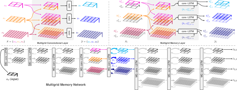
Multigrid organization, imposed on both spatial layout and connectivity, is the design principle that endows networks with this qualitatively new capacity for forming self-organized memory subsystems. Compared to almost all existing networks, a multigrid wiring pattern provides an exponentially more efficient routing topology among local components embedded within it. Ke et al. (2017) implement a multigrid variant of CNNs, demonstrating that efficient routing capacity enables the network to learn tasks that require attentional behavior. We distribute memory cells throughout such a network, and observe that this implicit capacity for attention translates into an implicit capacity for attention over memory read and write locations. Learned parameters govern how information flows through the network, what memory cells to update, and how to update them.

Our design philosophy starkly contrasts with recent neural memory architectures, including NTMs and the subsequent Differentiable Neural Computer (DNC) (Graves et al., 2016). These prior approaches isolate memory in an external storage bank, accessed via explicit addressing modes driven by custom hand-crafted controllers; they graft a von Neumann memory model onto a neural network. Instead, we intertwine memory units throughout the interior of a deep network. Memory is a first-class citizen, rather than a separate data store accessed via a special controller. We introduce a new kind of network layer—a multigrid memory layer—and use it as a stackable building block to create deep memory networks. Contrasting with simpler LSTMs, our memory is truly deep; accessing an arbitrary memory location requires passing through several layers. Figure 1 provides a visualization; we defer the full details to Section 3.

There are major benefits to our design strategy, in particular:

• Distributed, co-located memory and compute. Our memory layers incorporate convolutional and LSTM components. Stacking such layers, we create not only a memory network, but also a generalization of both CNNs and LSTMs. Our memory networks are standard networks with additional capabilities. Section 4 shows they can learn tasks that require performing classification alongside storage and recall.

  This unification also opens a design space for connecting our memory networks to each other, as well as to standard networks. Within a larger system, we can easily plug the internal state of our memory into a standard CNN—essentially granting that CNN read-only memory access. Sections 3 and 4 develop and experimentally validate two such memory interface approaches.

• Scalability. Distributing storage over a multigrid hierarchy allows us to instantiate large amounts of memory while remaining parameter-efficient. The low-level mechanism underlying memory access is convolution, and we inherit the parameter-sharing efficiencies of CNNs. Our filters act across a spatially organized collection of memory cells, rather than the spatial extent of an image. Increasing feature channels per memory cell costs parameters, but adding more cells incurs no such cost, decoupling memory size from parameter count. Connecting memory layers across spatial pyramid levels allows for growing memory spatial extent exponentially with network depth, while guaranteeing there is a pathway between the network input and every memory unit.

• Simplicity: implicit addressing, emergent subsystems. Our networks, once trained, behave like memory subsystems—this is an emergent phenomenon. Our design contains no explicit address calculation unit, no controller, and no attention mask computation. We take well known building blocks (i.e., convolution and LSTMs), wrap them in a multigrid wiring pattern, and achieve capabilities superior to those of the DNC, a far more complex design.

A diverse array of synthetic tasks serves as our experimental testbed. Mapping and localization, an inherently spatial task with relevance to robotics, is one focus. However, we avoid only experimenting with tasks naturally fit to the architecturally-induced biases of our memory networks. We also train them to perform algorithmic tasks, as well as natural language processing (NLP) tasks, previously used in analyzing the capabilities of NTMs and DNCs. Throughout all settings, DNC accuracy serves as a baseline. We observe significant advantages for multigrid memory, including:

• Long-term retention. On spatial mapping tasks, our network correctly remembers observations of an external environment collected over paths thousands of time steps long. Visualizing internal memory unit activations reveals an interpretable representation and algorithmic strategy our network learns for solving the problem. The DNC, in contrast, fails to master these tasks.

• Generality. On tasks decoupled from any notion of spatial geometry, such as associative recall or sorting (algorithmic), or question answering (NLP), our memory networks prove equally or more capable than DNCs.

Section 4 further elaborates on experimental results. Section 5 discusses implications: multigrid connectivity is a uniquely innovative design principle, as it allows qualitatively novel behaviors (attention) and subsystems (memory stores) to emerge from training simple components.

2 Related Work

An extensive history of work seeks to grant neural networks the ability to read and write memory (Das et al., 1992; 1993; Mozer & Das, 1993; Zeng et al., 1994; Hölldobler et al., 1997). Das et al. (1992) propose a neural pushdown automaton, which performs differential push and pop operations on external memory. Schmidhuber (1992) uses two feedforward networks: one produces context-dependent weights for the second, whose weights may change quickly and can be used as a form of memory. Schmidhuber (1993) proposes memory addressing in the form of a “self-referential” recurrent neural network that modifies its own weights.

Recurrent Long Short-Term Memory networks (LSTMs) (Hochreiter & Schmidhuber, 1997) have enabled significant progress on a variety of sequential prediction tasks, including machine translation (Sutskever et al., 2014), speech recognition (Graves et al., 2013), and image captioning (Donahue et al., 2017). LSTMs are Turing-complete (Siegelmann & Sontag, 1995) and are, in principle, capable of context-dependent storage and retrieval over long time periods (Hermans & Schrauwen, 2013). However, capacity for long-term read-write is sensitive to the training procedure (Collins et al., 2017) and is limited in practice.

Grid LSTMs (Kalchbrenner et al., 2015) arrange LSTM cells in a 2D or 3D grid, placing recurrent links along all axes of the grid. This sense of grid differs from our usage of multigrid, as the latter refers to links across a multiscale spatial layout. In Kalchbrenner et al. (2015)’s terminology, our multigrid memory networks are not Grid LSTMs, but are a variant of Stacked LSTMs (Graves et al., 2013).

To improve the long-term read-write abilities of recurrent networks, several modifications have been proposed. These include differentiable attention mechanisms (Graves, 2013; Bahdanau et al., 2014; Mnih et al., 2014; Xu et al., 2015) that provide a form of content-based memory addressing, pointer networks (Vinyals et al., 2015) that “point to” rather than blend inputs, and architectures that enforce independence among neurons within each layer (Li et al., 2018).

A number of methods augment the short- and long-term memory internal to recurrent networks with external “working” memory, in order to realize differentiable programming architectures that can learn to model and execute various programs (Graves et al., 2014; 2016; Weston et al., 2015b; Sukhbaatar et al., 2015; Joulin & Mikolov, 2015; Reed & de Freitas, 2015; Grefenstette et al., 2015; Kurach et al., 2015). Unlike our approach, these methods explicitly decouple memory from computation, mimicking a standard computer architecture. A neural controller (analogous to a CPU) interfaces with specialized external memory (e.g., random-access memory or tapes).

The Neural Turing Machine (Graves et al., 2014) augments neural networks with a hand-designed attention mechanism to read from and write to external memory in a differentiable fashion. This enables the NTM to learn to perform various algorithmic tasks, including copying, sorting, and associative recall. The Differential Neural Computer (Graves et al., 2016) improves upon the NTM with support for dynamic memory allocation and additional memory addressing modes. Without a sparsifying approximation, DNC runtime grows quadratically with memory due to the need to maintain the temporal link matrix. Our architecture has no such overhead, nor does it require maintaining any auxiliary state.

Other methods enhance recurrent layers with differentiable forms of a restricted class of memory structures, including stacks, queues, and dequeues (Grefenstette et al., 2015; Joulin & Mikolov, 2015). Gemici et al. (2017) augment structured dynamic models for temporal processes with various external memory architectures (Graves et al., 2014; 2016; Santoro et al., 2016).

Similar memory-explicit architectures have been proposed for deep reinforcement learning (RL) tasks. While deep RL has been applied to several challenging domains (Mnih et al., 2015; Hausknecht & Stone, 2015; Levine et al., 2016), most approaches reason over short-term state representations, which limits their ability to deal with partial observability inherent in many tasks. Several methods augment deep RL architectures with external memory to facilitate long-term reasoning. Oh et al. (2016) maintain a fixed number of recent states in memory and then read from the memory using a soft attention operation. Parisotto & Salakhutdinov (2018) propose a specialized write operator, together with a hand-designed 2D memory structure, both specifically crafted for navigation in maze-like environments.

Rather than learn when to write to memory (e.g., as done by NTM and DNC), Pritzel et al. (2017) continuously write the experience of an RL agent to a dictionary-like memory module queried in a key-based fashion (permitting large memories). Building on this framework, Fraccaro et al. (2018) augment a generative temporal model with a specialized form of spatial memory that exploits privileged information, including an explicit representation of the agent’s position.

Though we experiment with RL, our memory implementation contrasts with this past work. Our multigrid memory architecture jointly couples computation with memory read and write operations, and learns how to use a generic memory structure rather than one specialized to a particular task.

3 Multigrid Memory Architectures

A common approach to endowing neural networks with long-term memory builds memory addressing upon explicit attention mechanisms. Such attention mechanisms, independent of memory, are hugely influential in natural language processing (Vaswani et al., 2017). NTMs (Graves et al., 2014) and DNCs (Graves et al., 2016) address memory by explicitly computing a soft attention mask over memory locations. This leads to a design reliant on an external memory controller, which produces and then applies that mask when reading from or writing to a separate memory bank.

We craft a memory network without such strict division into modules. Instead, we propose a structurally uniform architecture that generalizes modern convolutional and recurrent designs by embedding memory cells within the feed-forward computational flow of a deep network. Convolutional neural networks and LSTMs (specifically, the convolutional LSTM variety (Xingjian et al., 2015)) exist as strict subsets of the full connection set comprising our multigrid memory network. We even encapsulate modern residual networks (He et al., 2016). Though omitted from diagrams (e.g., Figure 1) for the sake of clarity, we utilize residual connections linking the inputs of subsequent layers across the depth (not time) dimension of our memory networks.

In our design, memory addressing is implicit rather than explicit. We build upon an implicit capacity for attentional behavior inherent in a specific kind of network architecture. Ke et al. (2017) propose a multigrid variant of both standard CNNs and residual networks (ResNets). While their primary experiments concern image classification, they also present a striking result on a synthetic image-to-image transformation task: multigrid CNNs (and multigrid ResNets) are capable of learning to emulate attentional behavior. Their analysis reveals that the multigrid connection structure is both essential to and sufficient for enabling this phenomenon.

The underlying cause is that bi-directional connections across a scale-space hierarchy (Figure 1, left) create exponentially shorter signalling pathways between units at different locations on the spatial grid. Specifically, coarse-to-fine and fine-to-coarse connections between pyramids in subsequent layers allow a signal to hop up pyramid levels and back down again (and vice-versa). As a consequence, pathways connect any neuron in a given layer with every neuron located only $\mathcal{O}(\log(S))$ layers deeper, where $S$ is the spatial extent (diameter) of the highest-resolution grid (see Appendix A for a detailed analysis). In a standard convolutional network, this takes $\mathcal{O}(S)$ layers. These shorter pathways enable our convolutional architecture to approximate the behavior of a fully-connected network.

By replacing convolutional layers with convolutional LSTMs (Xingjian et al., 2015), we convert the inherent attentional capacity of multigrid CNNs into an inherent capacity for distributed memory addressing. Grid levels no longer correspond to operations on a multiresolution image representation, but instead correspond to accessing smaller or larger storage banks within a distributed memory hierarchy. Dynamic routing across scale space (in the multigrid CNN) now corresponds to dynamic routing into different regions of memory, according to a learned strategy.

3.1 Multigrid Memory Layer

Figure 1 diagrams both the multigrid convolutional layer of Ke et al. (2017) and our corresponding multigrid memory (MG-conv-LSTM) layer. Activations at a particular depth in our network consist of a pyramid $\mathcal{X}_{t}=\{(h^{x}_{j,t},c^{x}_{j,t})\}$, where $j$ indexes the pyramid level, $t$ indexes time, and $x$ is the layer. $h^{x}$ and $c^{x}$ denote the hidden state and memory cell contents of a convolutional LSTM (Xingjian et al., 2015), respectively. Following the construction of Ke et al. (2017), states $h^{x}$ at neighboring scales are resized and concatenated, with the resulting tensors fed as inputs to the corresponding scale-specific convolutional LSTM units in the next multigrid layer. The state associated with a conv-LSTM unit at a particular layer and level $(h^{y}_{j,t},c^{y}_{j,t})$ is computed from memory: $h^{y}_{j,t-1}$ and $c^{y}_{j,t-1}$, and input tensor: ${\uparrow}h^{x}_{j-1,t}\oplus h^{x}_{j,t}\oplus{\downarrow}h^{x}_{j+1,t}$, where $\uparrow$, $\downarrow$, and $\oplus$ denote upsampling, downsampling, and concatenation. Specifically, a multigrid memory layer (Figure 1, top right) operates as:

$$H^{x}_{j,t} :=({\uparrow}h^{x}_{j-1,t})\oplus(h^{x}_{j,t})\oplus({\downarrow}h^{x}_{j+1,t})$$

$$i_{j,t} :=\sigma(W^{xi}_{j}*H^{x}_{j,t}+W^{hi}_{j}*h^{y}_{j,t-1}+W^{ci}_{j}\circ c^{y}_{j,t-1}+b^{i}_{j})$$

$$f_{j,t} :=\sigma(W^{xf}_{j}*H^{x}_{j,t}+W^{hf}_{j}*h^{y}_{j,t-1}+W^{cf}_{j}\circ c^{y}_{j,t-1}+b^{f}_{j})$$

$$c^{y}_{j,t} :=f_{j,t}\circ c^{y}_{j,t-1}\!+i_{j,t}\circ\tanh(W^{xc}_{j}*H^{x}_{j,t}\!+\!W^{hc}_{j}\!*h^{y}_{j,t-1}\!+b^{c}_{j})$$

$$o^{y}_{j,t} :=\sigma(W^{xo}_{j}*H^{x}_{j,t}+W^{ho}_{j}*h^{y}_{j,t-1}+W^{co}_{j}\circ c^{y}_{j,t}+b^{o}_{j})$$

$$h^{y}_{j,t} :=o^{y}_{j,t}\circ\tanh(c^{y}_{j,t})$$

Superscripts denote variable roles (e.g., layer $x$ or $y$, and/or a particular parameter subtype for weights or biases). Subscripts index pyramid level $j$ and time $t$, $*$ denotes convolution, and $\circ$ the Hadamard product. Computation resembles Xingjian et al. (2015), with additional input tensor assembly, and repetition over output pyramid levels $j$. If a particular input pyramid level is not present in the architecture, it is dropped from the concatenation in the first step. Like Ke et al. (2017), downsampling ($\downarrow$) includes max-pooling. We utilize a two-dimensional memory geometry, and change resolution by a factor of two in each spatial dimension when moving up or down a pyramid level.

Connecting many such memory layers yields a memory network or distributed memory mesh, as shown in the bottom diagram of Figure 1. Note that a single time increment (from $t-1$ to $t$) involves running an entire forward pass of the network, propagating the input signal $a_{t}$ to the deepest layer $z_{t}$. Though not drawn here, we also incorporate batch normalization layers and residual connections along grids of corresponding resolution (i.e., from $h^{x}_{j,t}$ to $h^{y}_{j,t}$). These details mirror Ke et al. (2017). The convolutional nature of the multigrid memory architecture, together with its routing capability provides parameter-efficient implicit addressing of a scalable memory space.

3.2 Memory Interfaces

 

Figure 2: Memory interfaces. Top: Multiple readers (red, orange) and a single writer simultaneously manipulate a multigrid memory. Readers are multigrid CNNs; each convolutional layer views the hidden state of the corresponding grid in memory by concatenating it as an additional input. Bottom: Distinct encoder and decoder networks, each structured as a deep multigrid memory mesh, cooperate to perform a sequence-to-sequence task. We initialize the memory pyramid (LSTM internals) of each decoder layer by copying it from the corresponding encoder layer.

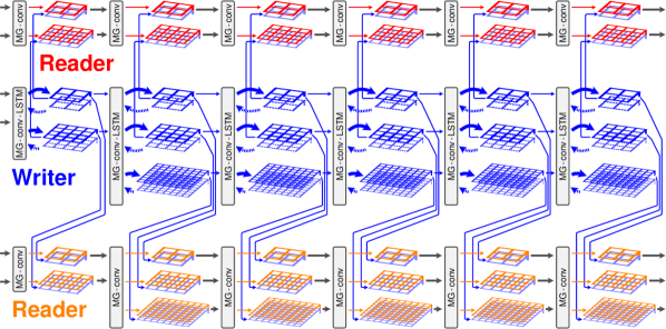
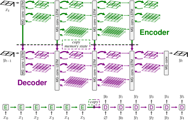
As our multigrid memory networks are multigrid CNNs plus internal memory units, we are able to connect them to other neural network modules as freely and flexibly as one can do with CNNs. Figure 2 diagrams a few such interface architectures, which we experimentally explore in Section 4.

In Figure 2 (top), multiple “threads”, two readers and one writer, simultaneously access a shared multigrid memory. The memory itself is located within the writer network (blue), which is structured as a deep multigrid convolutional-LSTM. The reader networks (red and orange), are merely multigrid CNNs, containing no internal storage, but observing the hidden state of the multigrid memory network.

Figure 2 (bottom) diagrams a deep multigrid analogue of a standard paired recurrent encoder and decoder. This design substantially expands the amount of memory that can be manipulated when learning sequence-to-sequence tasks.

4 Experiments

Figure 3: Mapping, localization, and exploration. An agent is comprised of a deep multigrid memory, and two deep multigrid CNNs (query and policy subnetworks), which have memory read access. Navigating a maze, the agent makes a local observation at each time step, and chooses a next action, receiving reward for exploring unseen areas. Given a random local patch, the query subnet must report all previously observed maze locations whose local observations match that patch. Subnet colors reflect those in Figure 2.

\begin{overpic}[height=57.81621pt]{figures/learned_representation2.png} \put(5.0,-3.0){{{{Observation: 3$\times$3, Query: 3$\times$3}}}} \put(55.0,-3.0){{{{Observation: 3$\times$3, Query: 9$\times$9}}}} \end{overpic}

Figure 4: Memory Visualization. Memory contents (hidden states $\{h_{t}\}$ on deepest, highest-resolution grid) mirror the map explored with spiral motion (top), vividly showing the interpretable strategy for self-organizing, implicit attentional addressing (reading/writing) of highly specific memory cells when training localization tasks, without having hand-designed attention mechanisms.

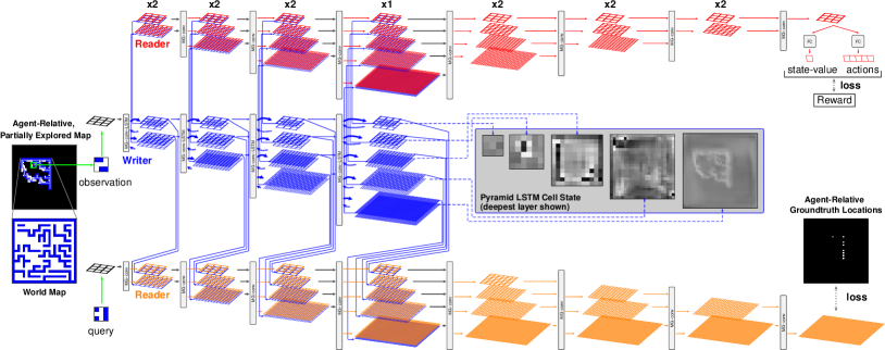
We evaluate our multigrid neural memory architecture on a diverse set of domains. We begin with a reinforcement learning-based navigation task, in which memory provides a representation of the environment (i.e., a map). To demonstrate the generalizability of our memory architecture on domains decoupled from spatial geometry, we also consider various algorithmic and NLP tasks previously used to evaluate the performance of NTMs and DNCs.

4.1 Mapping & Localization

We first consider a navigation problem, in which an agent explores a priori unknown environments with access to only observations of its immediate surroundings. Effective navigation requires maintaining a consistent representation of the environment (i.e., a map). Using memory as a form of map, an agent must learn where and when to perform write and read operations as it moves, while retaining the map over long time periods. This task mimics partially observable spatial navigation scenarios considered by memory-based deep reinforcement learning (RL) frameworks.

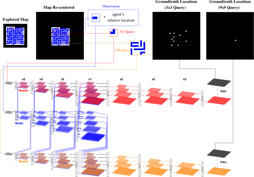
Problem Setup: The agent navigates an unknown $n\times n$ 2D maze and observes only the local $m\times m$ grid ($m\ll n$) centered at the agent’s position. It has no knowledge of its absolute position. Actions consist of one-step motion in the four cardinal directions. While navigating, we query the network with a randomly chosen, previously seen $k\times k$ patch ($m\leq k\ll n$) and ask it to identify every location matching that patch in the explored map. See Figure 3.

Multigrid Architecture: We use a deep multigrid network with multigrid memory and multigrid CNN subcomponents (Figure 3). Our memory (writer subnet) consists of seven MG-conv-LSTM layers, with pyramid spatial scales progressively increasing from $3\times 3$ to $48\times 48$. The reader, structured similarly, has an output attached to its deepest $48\times 48$ grid, and is tasked with answering localization queries. Section 4.2 experiments with an additional reader network that predicts actions, driving the agent to explore.

In order to understand the network’s ability to maintain a “map” of the environment in memory, we first consider a setting in which the agent executes a pre-defined navigation policy, and evaluate its localization performance. We consider different policies (spiraling outwards and a random walk), different patch sizes for observation and localization ($3\times 3$ or $9\times 9$), as well as different trajectory (path) lengths. We experiment in two regimes: small ($8$K) memory multigrid and DNC models, calibrated to the maximum trainable DNC size, and larger memory multigrid and convolutional-LSTM variants. We compare against:

• Differentiable Neural Computer (DNC) (Graves et al., 2016): see details in Appendix C.

• Ablated MG: a multigrid architecture variant including only the finest pyramid scale at each layer.

• ConvLSTM-deep: a network made of $23$ convolutional-LSTM layers, each on a $48\times 48$ grid, yielding the same total grid count as our $7$-layer multigrid network.

• ConvLSTM-thick: $7$ layers of convolutional-LSTMs acting on $48\times 48$ grids. We set channel counts to the sum of channels distributed across the corresponding pyramid layer of our large multigrid network.

We train each architecture using RMSProp. We search over learning rates in log scale from $10^{-2}$ to $10^{-4}$, and use $10^{-3}$ for multigrid and ConvLSTM, and $10^{-4}$ for DNC. We use randomly generated maps for training and testing. Training runs for $8\times 10^{6}$ steps with batch size $32$. Test set size is $5000$ maps. We used a pixel-wise cross-entropy loss over predicted and true locations (see Appendix B.1.2).

Table 1 reports performance in terms of localization accuracy on the test set. For the $25\times 25$ world in which the agent moves in a spiral (i.e., predictable) motion and the observation and query are $3\times 3$, our small multigrid network achieves near perfect precision ($99.33\%$), recall ($99.02\%$), and F-score ($99.17\%$), while all baselines struggle. Both ConvLSTM baselines fail to learn the task; simply stacking convolutional-LSTM units does not work. DNC performs similarly to Ablated MG in terms of precision ($\approx 77.6\%$), at the expense of a significant loss in recall ($14.50\%$). Instead, tasked with the simpler job of localization in a $15\times 15$ world, the performance of the DNC improves, yet its scores are still around $10\%$ lower than those of multigrid on the more challenging $25\times 25$ environment. For the $25\times 25$ map, efficiently addressing a large memory is required; the DNC’s explicit attention strategy appears to fall behind our implicit routing mechanism. Trying to compensate by augmenting the DNC with more memory is difficult: without a sparsifying approximation, the DNC’s temporal memory linkage matrix incurs a quadratic cost in memory size (see Appendix C). Our architecture has no such overhead, nor does it require maintaining auxiliary state. Even limiting multigrid to $8$K memory, it has no issue mastering the $25\times 25$ world.

Figure 4 visualizes the contents of the deepest and high-resolution LSTM block within the multigrid memory network of an agent moving in a spiral pattern. This memory clearly mirrors the contents of the true map. The network has learned a correct, and incidentally, an interpretable, procedure for addressing and writing memory.

Table 1: Mapping and localization. Our network significantly outperforms the DNC and other baselines. Efficient memory usage, enabled by multigrid connectivity, is essential; the DNC even fails to master smaller 15$\times$15 mazes. Our network retains memory over thousands of time-steps. Our localization subnet, trained on random motion, generalizes to queries for a policy-driven agent (last row).

Architecture	Params	Memory	World	Task Definition			Path	Localization Accuracy
	$(\times 10^{6})$	$(\times 10^{3})$	Map	FoV	Motion	Query	Length	Prec.	Recall	F
MG Mem+CNN	0.12	007.99	15$\times$15	3$\times$3	Spiral	3$\times$3	1169	99.79	99.88	99.83
DNC	0.75	008.00						91.09	87.67	89.35
MG Mem+CNN	0.17	007.99	25$\times$25				1529	99.33	99.02	99.17
DNC	0.68	008.00						77.63	14.50	24.44
MG Mem+CNN	0.65	076.97						99.99	99.97	99.98
Ablated MG	1.40	265.54						77.57	51.27	61.73
ConvLSTM-deep	0.38	626.69						43.42	03.52	06.51
ConvLSTM-thick	1.40	626.69						47.68	01.11	02.16
MG Mem+CNN	0.79	076.97	25$\times$25	3$\times$3	Spiral	9$\times$9	1529	97.34	99.50	98.41
	0.65	076.97		3$\times$3	Random	3$\times$3	1500	96.83	95.59	96.20
							1500	96.13	91.08	93.54
	0.66	078.12		9$\times$9	Random	9$\times$9	1500	92.82	87.60	90.14
	0.65	076.97		3$\times$3	Policy	3$\times$3	1000	95.65	90.22	92.86

Figure 5: Generalization of localization. Fixing parameters after training the query subnet on random motion (left), its localization loss remains low while training the exploration policy (middle), whose reward improves (right).

In more complex settings for motion type and query size (Table 1, bottom) our multigrid network remains accurate. It even generalizes to motions different from those on which it trained, including motion dictated by the learned policy that we describe shortly. Notably, even with the very long trajectory of $1500$ time steps, our proposed architecture has no issue retaining a large map memory.

4.2 Joint Exploration, Mapping, and Localization

We now consider a setting in which the agent learns an exploration policy via reinforcement, on top of a fixed mapping and localization network pre-trained with random walk motion. We implement the policy network as another multigrid reader, and leverage the pre-trained mapping and localization capabilities to learn a more effective policy.

We formulate exploration as a reinforcement learning problem: the agent receives a reward of $1$ when visiting a new space cell, $-1$ if it hits a wall, and $0$ otherwise. We use a discount factor $\gamma=0.99$, and train the multigrid policy network using A3C (Mnih et al., 2016).

Figure 5 (left) depicts the localization loss while pre-training the mapping and localization subnets. Freezing these subnets, we see that localization remains reliable (Figure 5, middle) while reinforcement learning the policy (Figure 5, right). The results demonstrate that the learned multigrid memory and query subnets generalize to trajectories that differ from those in their training dataset, as also conveyed in Table 1 (last row). Meanwhile, the multigrid policy network is able to utilize memory from the mapping subnet in order to learn an effective exploration policy. See Appendix E for visualizations of the exploratory behavior.

4.3 Algorithmic Tasks

We test the task-agnostic nature of our multigrid memory architecture by evaluating on a series of algorithmic tasks, closely inspired by those appearing in the original NTM work (Graves et al., 2014). For each of the following tasks, we consider two variants, increasing in level of difficulty. See Appendix B.2 for complete details.

Figure 6: Multigrid memory architectures learn significantly faster. Left: Maze localization task. Middle: Joint priority sort and classification. Right: Joint associative recall and classification.

Figure 7: MNIST recall. A random sequence of images followed by a repeat (green), output the class of the next image (red).

Table 2: Algorithmic tasks. Multigrid memory architectures achieve far lower error on the classification variants of priority sort and associative recall, while performing comparably to the DNC on the simpler versions of these tasks. Multigrid memory architectures also remain effective when dealing with long sequences.

	Architecture	Params	Memory	Item	List	Data	Task	Error Rate $\pm$ $\sigma$
		$(\times 10^{6})$	$(\times 10^{3})$	Size	Length
Standard Sequence	MG Enc+Dec	0.12	007.99	1$\times$9	20	Random	Priority Sort	0.0043$\pm$0.0009
	DNC	0.76	008.00			Patch		0.0039$\pm$0.0016
	MG Enc+Dec	0.29	007.56	28$\times$28	20	MNIST	Priority Sort	0.0864$\pm$0.0016
	DNC	1.05	008.00				+ Classify	0.1659$\pm$0.0188
	MG Mem+CNN	0.13	007.99	1$\times$9	10	Random	Assoc. Recall	0.0030$\pm$0.0002
	DNC	0.76	008.00			Patch		0.0044$\pm$0.0001
	MG Mem+CNN	0.21	007.56	28$\times$28	10	MNIST	Assoc. Recall	0.0736$\pm$0.0045
	DNC	0.90	008.00				+ Classify	0.2016$\pm$0.0161
Extended Sequence	MG Enc+Dec	0.89	076.97	1$\times$9	50	Random	Priority Sort	0.0067$\pm$0.0001
	MG Mem+CNN	0.65	076.97		20	Patch	Assoc. Recall	0.0056$\pm$0.0003

Figure 8: Multigrid memory encoder-decoder architecture for MNIST sorting. After processing the input sequence, the encoder (top) transfers memory into the decoder, which predicts the sequence of classes of the input digits in sorted order.

Figure 9: Multigrid memory architecture for question answering. 1D multigrid architecture is employed for question answering tasks. Input and output are $1\times 1\times 159$ tensors representing the word vectors. At each time step, the model receives a word input and generates the next word in the sequence.

Table 3: Question answering tasks. Despite using less memory, multigrid architecture surpasses DNC’s mean performance. While DNC performs slightly better in the best result, its high deviation from the mean shows that DNC is much more unstable compared to multigrid memory.

Architecture			Mean Result		Best Result
	Params	Memory	Mean Error $\pm$ $\sigma$	#Failed Tasks $\pm$ $\sigma$	Mean Error	#Failed Tasks
	$(\times 10^{6})$	$(\times 10^{3})$	(%)	(Error > 5%)	(%)	(Error > 5%)
MG Mem	1.00	02.86	$\hphantom{0}\bm{9.2\pm 1.0}$	$\hphantom{0}\bm{5.4\pm 1.4}$	7.5	4
DNC	0.89	16.38	$16.7\pm 7.6$	$11.2\pm 5.4$	$\bm{3.8}$	$\bm{2}$
EMN	N/A	N/A	N/A	N/A	7.5	6

Table 4: Complete question answering results. Shown are results for all $20$ question answering tasks.

Task	$\textrm{Mean}\pm\sigma$
	MG Mem	DNC
single supporting fact	$\hphantom{0}\bf{0.3\pm 0.3}\hphantom{0}$	$\hphantom{0}9.0\pm 12.6$
two supporting facts	$\bf{27.4\pm 7.8}\hphantom{0}$	$39.2\pm 20.5$
three supporting facts	$51.8\pm 5.0\hphantom{0}$	$\bf{39.6\pm 16.4}$
two argument relations	$\hphantom{0}\bf{0.1\pm 0.1}\hphantom{0}$	$\hphantom{0}0.4\pm 0.7\hphantom{0}$
three argument relations	$\hphantom{0}3.4\pm 0.6\hphantom{0}$	$\hphantom{0}\bf{1.5\pm 1.0}\hphantom{0}$
yes/no questions	$\hphantom{0}\bf{1.7\pm 1.0}\hphantom{0}$	$\hphantom{0}6.9\pm 7.5\hphantom{0}$
counting	$\hphantom{0}\bf{5.2\pm 2.1}\hphantom{0}$	$\hphantom{0}9.8\pm 7.0\hphantom{0}$
lists/sets	$\hphantom{0}\bf{4.5\pm 1.3}\hphantom{0}$	$\hphantom{0}5.5\pm 5.9\hphantom{0}$
simple negation	$\hphantom{0}\bf{0.8\pm 0.6}\hphantom{0}$	$\hphantom{0}7.7\pm 8.3\hphantom{0}$
indefinite knowledge	$\hphantom{0}\bf{5.9\pm 1.9}\hphantom{0}$	$\hphantom{0}9.6\pm 11.4$
basic coreference	$\hphantom{0}\bf{0.5\pm 0.2}\hphantom{0}$	$\hphantom{0}3.3\pm 5.7\hphantom{0}$
conjunction	$\hphantom{0}\bf{0.4\pm 0.3}\hphantom{0}$	$\hphantom{0}5.0\pm 6.3\hphantom{0}$
compound coreference	$\hphantom{0}\bf{0.1\pm 0.1}\hphantom{0}$	$\hphantom{0}3.1\pm 3.6\hphantom{0}$
time reasoning	$22.0\pm 1.9\hphantom{0}$	$\bf{11.0\pm 7.5}\hphantom{0}$
basic deduction	$\bf{0.4\pm 0.5}$	$27.2\pm 20.1$
basic induction	$\bf{51.6\pm 2.9}\hphantom{0}$	$53.6\pm 1.9\hphantom{0}$
positional reasoning	$\hphantom{0}\bf{4.6\pm 2.1}\hphantom{0}$	$32.4\pm 8.0\hphantom{0}$
size reasoning	$\hphantom{0}\bf{1.7\pm 0.7}\hphantom{0}$	$\hphantom{0}4.2\pm 1.8\hphantom{0}$
path finding	$\bf{1.4\pm 1.2}$	$64.6\pm 37.4$
agents motivations	$\hphantom{0}0.2\pm 0.4\hphantom{0}$	$\hphantom{0}\bf{0.0\pm 0.1}\hphantom{0}$
Mean Error (%)	$\hphantom{0}\bf{9.2\pm 1.0}\hphantom{0}$	$16.7\pm 7.6\hphantom{0}$
Failed Tasks (Error > 5%)	$\hphantom{0}\bf{5.4\pm 1.4}\hphantom{0}$	$11.2\pm 5.4\hphantom{0}$

Priority Sort. In the first non-visual variant, the network receives a sequence of twenty $9$-dimensional vectors, along with their priority. The task is to output the sequence of vectors in order of their priority. Training and testing use randomly generated data. Training takes $2\times 10^{6}$ steps, batch size $32$, and testing uses $5000$ sequences. Results are computed over $10$ runs. We tune hyperparameters as done for the mapping task. We structure our model as an encoder-decoder architecture (Figure 2, bottom). Our network performs equivalently to DNC with equal memory, with both achieving near-perfect performance (Table 2).

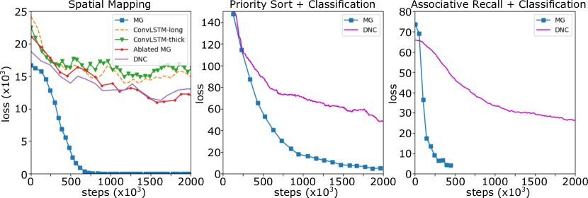
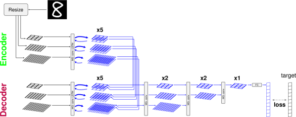
The second variant extends the priority sort to require recognition capability. The input is a sequence of twenty $28\times 28$ MNIST images (Lecun et al., 1998). The goal is to output the class of the input images in increasing order. A sample encoder-decoder architecture employed for this task is presented in Figure 8. Table 2 reveals that our architecture achieves much lower error rate compared to DNC on this task (priority sort + classification), while also learning faster (Figure 6) and with less memory.

Associative Recall. In the first formulation, the network receives a sequence of ten $9$-element random vectors, followed by a second instance of one of the first nine vectors. The task is to output the vector that immediately followed the query in the input sequence. We demonstrate this capability using the multigrid reader/writer architecture (Figure 2, top). Training is similar to the sorting task. Table 2 shows that both DNC and our architecture achieve near-zero error rates.

In the second variant, the input is a sequence of ten $28\times 28$ randomly chosen MNIST images (Lecun et al., 1998), where the network needs to output the class of the image immediately following the query (Figure 7). As shown in Table 2 and Figure 6, our multigrid memory network performs this task with significantly greater accuracy than the DNC, and also learns in fewer training steps.

To further test the ability of multigrid memory architectures to deal with longer sequences, we experimented with sorting and associative recall with sequence length of $50$ and $20$, respectively. As can be seen in Table 2, multigrid memory architectures remain effective with near-zero error rates.

The harder variants of both priority sort and associative recall require a combination of memory and a pattern recognition capability. The success of multigrid memory networks (and notable poor performance of DNCs), demonstrates that they are a unique architectural innovation. They are capable of learning to simultaneously perform representational transformations and utilize a large distributed memory store. Furthermore, as Figure 6 shows, across all difficult tasks, including mapping and localization, multigrid memory networks train substantially faster and achieve substantially lower loss than all competing methods.

4.4 Question Answering

To further investigate the generalizability of our multigrid memory architecture well beyond spatial reasoning, we evaluate its performance on bAbI Weston et al. (2015a), which consist of $20$ question answering tasks corresponding to diverse aspects of natural language understanding. For each task, the dataset contains $10000$ questions for training and $1000$ for testing. For parameter-efficiency, we employ a 1D multigrid architecture for this task, as shown in Figure 9. Results are shown in Table 3. Despite having only a fraction of the memory available to the DNC ($2.86$K v.s. $16.38$K), on average our architecture outperforms the DNC in terms of both mean error rate ($9.2\%$ v.s. $16.7\%$) and mean failed tasks ($5.4$ v.s. $11.2$). On best results, while DNC performs slightly better, multigrid memory still outperforms EMN (Sukhbaatar et al., 2015) with fewer failed tasks. Complete results for all tasks are presented in Table 4. These results not only demonstrate the adaptability of multigrid memory, but are also a testament to our design’s effectiveness. See Appendix B.3 for further details.

5 Conclusion

Multigrid memory represents a radical new approach to augmenting networks with long-term, large-scale storage. A simple principle, multigrid connectivity, underlies our model. Residual networks He et al. (2016), which provide shortcut pathways across depth, have had enormous impact, allowing very deep networks to be trained by facilitating gradient propagation. Multigrid wiring is complementary, improving connectivity across an orthogonal aspect of the network: the spatial dimension. Its impact is equally significant: multigrid wiring exponentially improves internal data routing efficiency, allowing complex behaviors (attention) and coherent memory subsystems to emerge from training simple components. Our results are cause to rethink the prevailing design principles for neural network architectures.

Acknowledgments. We thank Gordon Kindlmann for his support in pursuing this project, Chau Huynh for her help with the code, and Pedro Savarese and Hai Nguyen for fruitful discussions. The University of Chicago CERES Center contributed to the support of Tri Huynh. This work was supported in part by the National Science Foundation under grant IIS-1830660.

Appendix A Information Routing

Figure 10: Information routing. Top: Paths depicting information flow in a multigrid architecture. Progressing from one layer to the next, information flows between grids at the same level (via convolution, green), as well as to adjacent grids at higher resolution (via upsampling and convolution, red) and lower resolution (via downsampling and convolution, orange). Information from a sample location $(26,26)$ (blue) of the source grid at [layer 1, level 4] can be propagated to all locations rendered in blue in subsequent layers and levels, following the indicated paths (among others). Information quickly flows from finer levels to coarser levels, and then to any location in just a few layers. Receptive field size grows exponentially with depth. In practice, the routing strategy is emergent—routing is determined by the learned network parameters (convolutional filters). Multigrid connectivity endows the network with the potential to quickly route from any spatial location to any other location just a few layers deeper. Bottom: Information flow in a standard architecture. Without multigrid connections, information from the same source location is propagated much more slowly across network layers. Receptive fields expand at a constant rate with depth, compared to the multigrid network’s exponential growth.

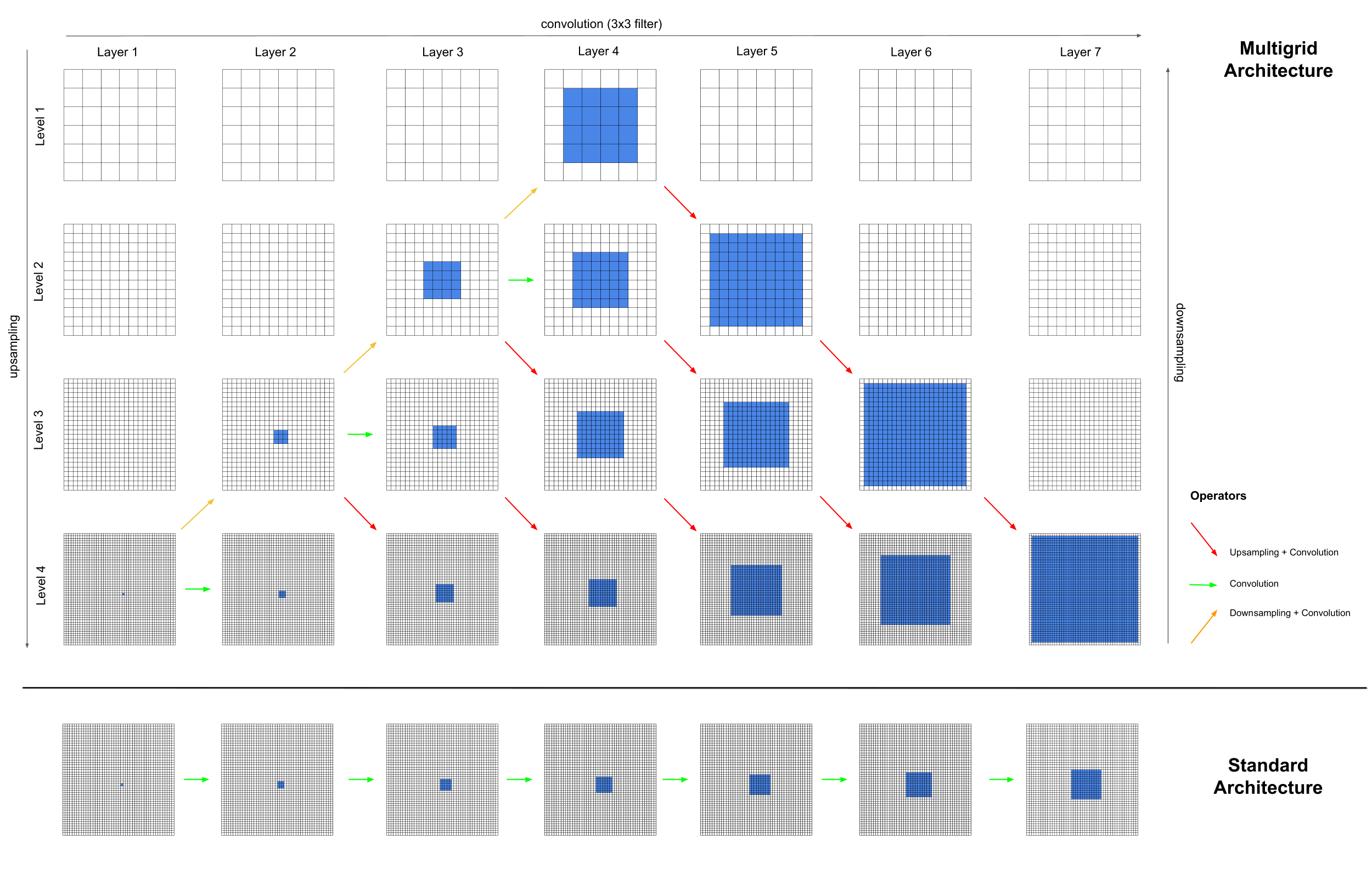
Proposition 1: For the setup in Figure 10, suppose that the convolutional kernel size is $3\times 3$, and upsampling is $2\times$ nearest-neighbor sampling. Consider location $(1,1)$ of the source grid at [layer $1$, level $1$]. For a target grid at [layer $m$, level $n$], where $m\geq n$, the information from the source location can be routed to any location $(i,j)$, where $1\leq i$, $j\leq(m-n+2)\cdot 2^{n-1}-1$.

Proof of Proposition 1: Induction proof on level $n$.

• For level $n=1$: Each convolution of size $3\times 3$ can direct information from a location $(i,j)$ at layer $k$ to any of its immediate neighbors $(i^{\prime},j^{\prime})$ where $i-1\leq i^{\prime}\leq i+1$, $j-1\leq j^{\prime}\leq j+1$ in layer $k+1$. Therefore, convolutional operations can direct information from location $(1,1)$ in layer $1$ to any locations $(i^{\prime},j^{\prime})$ in layer $k=m$ where $1\leq i^{\prime}$ , $j^{\prime}\leq m=(m-1+2)\cdot 2^{0}-1=(m-n+2)\cdot 2^{n-1}-1$.

• Assume the proposition is true for level $n$ ($\forall m\geq n$), we show that it is true for level $n+1$. Consider any layer $m+1$ in level $n+1$, where $m+1\geq n+1$:

  We have, $m+1\geq n+1\Rightarrow m\geq n$. Therefore, we have that at [layer $m$, level $n$], the information from the source location can be routed to any location $(i,j)$, where $1\leq i$, $j\leq(m-n+2)\cdot 2^{n-1}-1$. Now, consider the path from [layer $m$, level $n$] to [layer $m+1$, level $n+1$]. This path involves the upsampling followed by a convolution operator, as illustrated in Figure 10.

  Nearest-neighbor upsampling directly transfers information from index $i$ to $2\cdot i$ and $2\cdot i-1$, and $j$ to $2\cdot j$ and $2\cdot j-1$ by definition. For simplicity, first consider index $i$ separately. By transferring to $2\cdot i$, information from location $1\leq i\leq(m-n+2)\cdot 2^{n-1}-1$ in level $n$ will be transferred to all even indices in $[2,((m-n+2)\cdot 2^{n-1}-1)\cdot 2]$ at level $n+1$. By transferring to $2\cdot i-1$, information from location $1\leq i\leq(m-n+2)\cdot 2^{n-1}-1$ in level $n$ will be transferred to all odd indices in $[1,((m-n+2)\cdot 2^{n-1}-1)\cdot 2-1]$ at level $n+1$. Together, with $2\cdot i$ and $2\cdot i-1$ transferring, the nearest-neighbor upsampling transfers information from location $1\leq i\leq(m-n+2)\cdot 2^{n-1}-1$ in level $n$ to all indices in $[1,((m-n+2)\cdot 2^{n-1}-1)\cdot 2]$ at level $n+1$.

  Furthermore, the following convolution operator with $3\times 3$ kernel size can continue to transfer information from $[1,((m-n+2)\cdot 2^{n-1}-1)\cdot 2]$ to $[1,((m-n+2)\cdot 2^{n-1}-1)\cdot 2+1]$ at level $n+1$. We have $((m-n+2)\cdot 2^{n-1}-1)\cdot 2+1=(m+1-(n+1)+2)\cdot 2^{n}-1$. Taking together indices $i$ and $j$, information from location $(i,j)$ where $1\leq i$, $j\leq(m-n+2)\cdot 2^{n-1}-1$ in level $n$ can be transferred to $(i\textquoteright,j\textquoteright)$ in level $n+1$, where $1\leq i^{\prime}$, $j^{\prime}\leq(m+1-(n+1)+2)\cdot 2^{n}-1$. $\blacksquare$

Appendix B Experiment Details

Figure 11: Multigrid memory writer-reader(s) architecture for spatial navigation. At each time step, the agent moves to a new location and observes the surrounding $3\times 3$ patch. The writer receives this $3\times 3$ observation along with the agent’s relative location (with respect to the starting point), updating the memory with this information. Two readers receive randomly chosen $3\times 3$ and $9\times 9$ queries, view the current map memory built by the writer, and infer the possible locations of those queries.

B.1 Spatial Navigation

B.1.1 Architecture

All experiments related to spatial navigation tasks use multigrid writer-reader(s) architectures. Figure 11 visualizes this architecture and problem setup. At each time step during training, the agent takes a one-step action (e.g., along a spiral trajectory) and observes its $3\times 3$ surroundings. This observation, together with its location relative to the starting point, are fed into the writer, which must learn to update its memory. The agent has no knowledge of its absolute location in the world map. Two random $3\times 3$ and $9\times 9$ patches within the explored map are presented to the agent as queries (some experiments use only $3\times 3$ queries). These queries feed into two readers, each viewing the same memory built by the writer; they must infer which previously seen locations match the query. Since the agent has no knowledge of its absolute location in the world map, the agent builds a map relative to its initial position (map re-centered in Figure 11) as it navigates.

During training, the writer learns to organize and update memory from localization losses simultaneously backpropagated from the two readers. During inference, only the writer updates the memory at each time step, and the readers simply view (i.e., without modification) the memory to infer the query locations. It is also worth noting that only $3\times 3$ patches are fed into the writer at each time step; the agent never observes a $9\times 9$ patch. However, the agent successfully integrates information from the $3\times 3$ patches into a coherent map memory in order to correctly answer queries much larger than its observations. Figure 4 shows that this learned memory strikingly resembles the actual world map.

B.1.2 Loss

Given predicted probabilities and the ground-truth location mask (Figure 11), we employ a pixel-wise cross-entropy loss as the localization loss. Specifically, letting $S$ be the set of pixels, $p_{i}$ be the predicted probability at pixel $i$, and $y_{i}$ be the binary ground-truth at pixel $i$, the pixel-wise cross-entropy loss is computed as follows:

$$-\sum_{i\in S}y_{i}\log(p_{i})+(1-y_{i})\log(1-p_{i})$$ (1)

B.2 Algorithmic Tasks

B.2.1 Architecture

Priority Sort Tasks:

We employ encoder-decoder architectures for the priority sort tasks.

• Standard variant. The encoder is a 5-layer multigrid memory architecture, structured similar to the writer in Figure 11, progressively scaling $3\times 3$ inputs at the coarsest resolution into $24\times 24$ resolution. For the decoder, the first half of the layers (MG-conv-LSTM) resemble the encoder, while the second half employ MG-conv layers to progressively scale down the output to $3\times 3$.

• MNIST sort + classification. Figure 8 depicts the encoder-decoder architecture for the MNIST variant.

Associative Recall Tasks:

We employ writer-reader architectures for the associative recall tasks. The architectures are similar to those for the spatial navigation and priority sort tasks depicted in Figure 11, with some modifications appropriate to the tasks:

• Standard variant. In the standard version of the task, the writer architecture is similar to the encoder in the standard variant of the priority sort task. For the reader, after progressing to the finest resolution corresponding to the memory in the writer, the second half of MG-conv layers progressively scale down the output to $3\times 3$ to match the expected output size.

• MNIST recall + classification. For the MNIST variant, we resize the $28\times 28$ images to three scales from $3\times 3$ to $12\times 12$ and maintain the same three-scale structure for five layers of the writer. The writer architecture is similar to the encoder architecture in MNIST priority sort task, as depicted in Figure 8. The reader for the MNIST variant is similar to the reader in the standard variant, with the final layer followed by a fully connected layer to produce a 10-way prediction vector over MNIST classes.

B.2.2 Loss

Standard variants:

We use pixel-wise cross-entropy loss for the standard variants, as described in Section B.1.2.

MNIST variants:

For MNIST variants, we use cross-entropy loss over a softmax prediction of the classes. Specifically, letting $C$ be the set of available classes, $p_{c}$ the softmax output for class $c$, and $y$ a one-hot vector of the ground-truth label, we compute the loss as:

$$-\sum_{c\in C}y_{c}\log(p_{c})$$ (2)

B.3 Question Answering

B.3.1 Architecture

We employ a 1D multigrid memory architecture for question answering tasks, where the spatial dimensions progressively scale from $1\times 1$ to $1\times 16$ through MG-conv-LSTM layers, and gradually scale back to $1\times 1$ through MG-conv layers, as demonstrated in Figure 9. Inputs and outputs are $1\times 1\times\lvert V\rvert$ tensors representing the word vectors, where $V$ is the set of words in the vocabulary and $\lvert V\rvert=159$. All 20 question answering tasks are jointly trained, with batch size 1, and sequence-wise normalization. At each time step, the model receives a word input and generates the next word in the sequence. During training, only the losses from words corresponding to answers are backpropagated, others are masked out, as specified next.

B.3.2 Loss

Let $V$ be the set of words in the vocabulary, and $y\in\{0,1\}^{\lvert V\rvert}$ be a one-hot vector that represents the ground-truth word. For a word sequence $S$, we define a mask $m$ as:

$$m_{i}=\begin{cases}1&\text{if word $i$ in the sequence $S$ is an answer}\\ 0&\text{otherwise}\end{cases}$$ (3)

Letting $p\in(0,1)^{\lvert V\rvert}$ be the softmax output, we compute the loss for question answering as follows:

$$-\sum_{i=1}^{\lvert S\rvert}m_{i}\sum_{j=1}^{\lvert V\rvert}y_{j}^{i}\log(p_{j}^{i})$$ (4)

Appendix C DNC Details

Figure 12: Visualization of DNC memory in mapping task. Due to its defined addressing mechanism, the DNC always allocates a new continuous memory slot at each time-step. It does not appear to maintain an interpretable structure of the map.

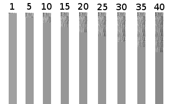
We use the official DNC implementation (https://github.com/deepmind/dnc), with $5$ controller heads ($4$ read heads and $1$ write head). For spatial navigation and algorithmic tasks, we use a memory vector of $16$ elements, and $500$ memory slots ($8$K total), which is the largest memory size permitted by GPU resource limitations. Controllers are LSTMs, with hidden state sizes chosen to make total parameters comparable to other models in Table 1 and Table 2. DNC imposes a relatively small cap on the addressable memory due to the quadratic cost of the temporal linkage matrix (https://github.com/deepmind/dnc/blob/master/dnc/addressing.py#L163).

A visualization of DNC memory in the spatial mapping task ($15\times 15$ map) is provided in Figure 12.

For question answering tasks, the DNC memory is comprised of $256$ memory slots, with a $64$-element vector for each slot ($16,384$ total). The use of a smaller number of memory slots and batch size allows for the allocation of larger total memory.

Appendix D Runtime

On spatial mapping (with $15\times 15$ world map), the runtimes for one-step inference with the Multigrid Memory architecture ($0.12$ M parameters and $8$ K memory) and DNC ($0.75$ M parameters and $8$ K memory) are ($\text{mean}\pm\text{std}$): $0.018\pm 0.003$ seconds and $0.017\pm 0.001$ seconds, respectively. These statistics are computed over $10$ runs on a NVIDIA Geforce GTX Titan X.

Appendix E Demos

• Instructions for interpreting the video demos:
  https://drive.google.com/file/d/18gvQRhNaEbdiV8oNKOsuUXpF75FEHmgG

• Mapping & localization in spiral trajectory, with $3\times 3$ queries:
  https://drive.google.com/file/d/1VGPGHqcNXBRdopMx11_wy9XoJS7REXbd

• Mapping & localization in spiral trajectory, with $3\times 3$ and $9\times 9$ queries:
  https://drive.google.com/file/d/18lEba0AzpLdAqHhe13Ah3fL2b4YEyAmF

• Mapping & localization in random trajectory:
  https://drive.google.com/file/d/19IX93ppGeQ56CqpgvN5MJ2pCl46FjgkO

• Joint exploration, mapping & localization:
  https://drive.google.com/file/d/1UdTmxUedRfC-E6b-Kz-1ZqDRnzXV4PMM

References

- Bahdanau et al. (2014) Bahdanau, D., Cho, K., and Bengio, Y. Neural machine translation by jointly learning to align and translate. arXiv:1409.0473, 2014.
- Collins et al. (2017) Collins, J., Sohl-Dickstein, J., and Sussillo, D. Capacity and trainability in recurrent neural networks. ICLR, 2017.
- Das et al. (1992) Das, S., Giles, C. L., and Sun, G.-Z. Learning context-free grammars: Capabilities and limitations of a recurrent neural network with an external stack memory. In CogSci, 1992.
- Das et al. (1993) Das, S., Giles, C. L., and Sun, G.-Z. Using prior knowledge in an NNPDA to learn context-free languages. In NIPS, 1993.
- Donahue et al. (2017) Donahue, J., Hendricks, L. A., Rohrbach, M., Venugopalan, S., Guadarrama, S., Saenko, K., and Darrell, T. Long-term recurrent convolutional networks for visual recognition and description. IEEE Transactions on Pattern Analysis and Machine Intelligence, 2017.
- Fraccaro et al. (2018) Fraccaro, M., Rezende, D. J., Zwols, Y., Pritzel, A., Eslami, S. M. A., and Viola, F. Generative temporal models with spatial memory for partially observed environments. ICML, 2018.
- Gemici et al. (2017) Gemici, M., Hung, C.-C., Santoro, A., Wayne, G., Mohamed, S., Rezende, D. J., Amos, D., and Lillicrap, T. Generative temporal models with memory. arXiv:1702.04649, 2017.
- Graves (2013) Graves, A. Generating sequences with recurrent neural networks. arXiv:1308.0850, 2013.
- Graves et al. (2013) Graves, A., rahman Mohamed, A., and Hinton, G. Speech recognition with deep recurrent neural networks. In IEEE International Conference on Acoustics, Speech and Signal Processing, 2013.
- Graves et al. (2014) Graves, A., Wayne, G., and Danihelka, I. Neural turing machines. arXiv:1410.5401, 2014.
- Graves et al. (2016) Graves, A., Wayne, G., Reynolds, M., Harley, T., Danihelka, I., Grabska-Barwińska, A., Colmenarejo, S. G., Grefenstette, E., Ramalho, T., Agapiou, J., Badia, A. P., Hermann, K. M., Zwols, Y., Ostrovski, G., Cain, A., King, H., Summerfield, C., Blunsom, P., Kavukcuoglu, K., and Hassabis, D. Hybrid computing using a neural network with dynamic external memory. Nature, 2016.
- Grefenstette et al. (2015) Grefenstette, E., Hermann, K. M., Suleyman, M., and Blunsom, P. Learning to transduce with unbounded memory. In NIPS, 2015.
- Hausknecht & Stone (2015) Hausknecht, M. and Stone, P. Deep recurrent Q-learning for partially observable MDPs. In AAAI Fall Symposium, 2015.
- He et al. (2016) He, K., Zhang, X., Ren, S., and Sun, J. Deep residual learning for image recognition. CVPR, 2016.
- Hermans & Schrauwen (2013) Hermans, M. and Schrauwen, B. Training and analysing deep recurrent neural networks. NIPS, 2013.
- Hochreiter & Schmidhuber (1997) Hochreiter, S. and Schmidhuber, J. Long short-term memory. Neural Computation, 1997.
- Hölldobler et al. (1997) Hölldobler, S., Kalinke, Y., and Lehmann, H. Designing a counter: Another case study of dynamics and activation landscapes in recurrent networks. In Annual Conference on Artificial Intelligence, 1997.
- Joulin & Mikolov (2015) Joulin, A. and Mikolov, T. Inferring algorithmic patterns with stack-augmented recurrent nets. In NIPS, 2015.
- Kalchbrenner et al. (2015) Kalchbrenner, N., Danihelka, I., and Graves, A. Grid long short-term memory. arXiv:1507.01526, 2015.
- Ke et al. (2017) Ke, T.-W., Maire, M., and Yu, S. X. Multigrid neural architectures. CVPR, 2017.
- Kurach et al. (2015) Kurach, K., Andrychowicz, M., and Sutskever, I. Neural random-access machines. arXiv:1511.06392, 2015.
- Lecun et al. (1998) Lecun, Y., Bottou, L., Bengio, Y., and Haffner, P. Gradient-based learning applied to document recognition. Proceedings of the IEEE, 1998.
- Levine et al. (2016) Levine, S., Finn, C., Darrell, T., and Abbeel, P. End-to-end training of deep visuomotor policies. The Journal of Machine Learning Research, 2016.
- Li et al. (2018) Li, S., Li, W., Cook, C., Zhu, C., and Gao, Y. Independently recurrent neural network (indrnn): Building a longer and deeper rnn. CVPR, 2018.
- Mnih et al. (2014) Mnih, V., Heess, N., Graves, A., et al. Recurrent models of visual attention. In NIPS, 2014.
- Mnih et al. (2015) Mnih, V., Kavukcuoglu, K., Silver, D., Rusu, A. A., Veness, J., Bellemare, M. G., Graves, A., Riedmiller, M., Fidjeland, A. K., Ostrovski, G., et al. Human-level control through deep reinforcement learning. Nature, 2015.
- Mnih et al. (2016) Mnih, V., Badia, A. P., Mirza, M., Graves, A., Lillicrap, T. P., Harley, T., Silver, D., and Kavukcuoglu, K. Asynchronous methods for deep reinforcement learning. ICML, 2016.
- Mozer & Das (1993) Mozer, M. C. and Das, S. A connectionist symbol manipulator that discovers the structure of context-free languages. In NIPS, 1993.
- Oh et al. (2016) Oh, J., Chockalingam, V., Singh, S., and Lee, H. Control of memory, active perception, and action in Minecraft. arXiv:1605.09128, 2016.
- Parisotto & Salakhutdinov (2018) Parisotto, E. and Salakhutdinov, R. Neural map: Structured memory for deep reinforcement learning. ICLR, 2018.
- Pritzel et al. (2017) Pritzel, A., Uria, B., Srinivasan, S., Puigdomenech, A., Vinyals, O., Hassabis, D., Wierstra, D., and Blundell, C. Neural episodic control. ICML, 2017.
- Reed & de Freitas (2015) Reed, S. and de Freitas, N. Neural programmer-interpreters. arXiv:1511.06279, 2015.
- Santoro et al. (2016) Santoro, A., Bartunov, S., Botvinick, M., Wierstra, D., and Lillicrap, T. One-shot learning with memory-augmented neural networks. arXiv:1605.06065, 2016.
- Schmidhuber (1992) Schmidhuber, J. Learning to control fast-weight memories: An alternative to dynamic recurrent networks. Neural Computation, 1992.
- Schmidhuber (1993) Schmidhuber, J. A ‘self-referential’weight matrix. In ICANN, 1993.
- Siegelmann & Sontag (1995) Siegelmann, H. T. and Sontag, E. D. On the computational power of neural nets. Journal of computer and system sciences, 1995.
- Sukhbaatar et al. (2015) Sukhbaatar, S., Weston, J., Fergus, R., et al. End-to-end memory networks. In NIPS, 2015.
- Sutskever et al. (2014) Sutskever, I., Vinyals, O., and Le, Q. V. Sequence to sequence learning with neural networks. In NIPS, 2014.
- Vaswani et al. (2017) Vaswani, A., Shazeer, N., Parmar, N., Uszkoreit, J., Jones, L., Gomez, A. N., Kaiser, Ł., and Polosukhin, I. Attention is all you need. NeurIPS, 2017.
- Vinyals et al. (2015) Vinyals, O., Fortunato, M., and Jaitly, N. Pointer networks. In NIPS, 2015.
- Weston et al. (2015a) Weston, J., Bordes, A., Chopra, S., Rush, A. M., van Merriënboer, B., Joulin, A., and Mikolov, T. Towards AI complete question answering: A set of prerequisite toy tasks. arXiv:1502.05698, 2015a.
- Weston et al. (2015b) Weston, J., Chopra, S., and Bordes, A. Memory networks. ICLR, 2015b.
- Xingjian et al. (2015) Xingjian, S., Chen, Z., Wang, H., Yeung, D.-Y., Wong, W.-K., and Woo, W.-c. Convolutional LSTM network: A machine learning approach for precipitation nowcasting. NIPS, 2015.
- Xu et al. (2015) Xu, K., Ba, J., Kiros, R., Cho, K., Courville, A., Salakhutdinov, R., Zemel, R., and Bengio, Y. Show, attend and tell: Neural image caption generation with visual attention. arXiv:1502.03044, 2015.
- Zeng et al. (1994) Zeng, Z., Goodman, R. M., and Smyth, P. Discrete recurrent neural networks for grammatical inference. IEEE Transactions on Neural Networks, 1994.