Parameter estimation in an elliptic problem.

Abstract.

A new variational approach to solve the problem of estimating the (possibly discontinuous) coefficient functions $p$, $q$ and $f$ in elliptic equations of the form $-\nabla\cdot(p(x)\nabla u)+\lambda q(x)u=f$, $x\in\Omega\subset\mathbb{R}^{n}$, from a knowledge of the solutions $u_{\lambda}$.

Example 1.

Parameter identification.
By parameter identification one usually denotes the problem of reconstructing the unknown coefficients in a partial differential equation from (indirect) measurements of the solution or a noisy solution. A simple example is the following model from groundwater filtration, which is modeled through the following elliptic equation

(1) $$-\nabla.(p\nabla u)=f,$$

in $\Omega\subset\mathbb{R}^{d}$, where $u$ is the unknown, $f$ a given source, and $p$ the hydraulic permittivity. The direct problem consists in solving the partial differential equation for $u$, given a $p$ and suitable boundary conditions on $\partial\Omega$. The inverse problem consists in reconstructing the unknown parameter $p$ on $\Omega$ given a noisy measurement of the solution,

(2) $$u_{\delta}(x)=u(x)+\epsilon_{\delta}(x),\hskip 28.45274ptx\in\Omega.$$

If the solution of the direct problem is unique for each parameter $p$, which is the case for the groundwater filtration problem with appropriate boundary conditions, then one can introduce the parameter-to-solution map, $p\rightarrow u_{p}$, where $u_{p}$ is the solution to the direct problem given a specific $p$. Note that even if the direct problem is linear (for $u$), the inverse problem and the parameter-to-output map are usually non-linear. For example, in the ground water filtration problem we have $u_{2p}=\frac{1}{2}u_{p}$, and not $u_{2p}=2u_{p}$ and hence, the problem is not linear.

The uniqueness question for parameter identification problems is usually denoted as identifiability. For example, if $\Omega=[0,1]$ then integrating equation (1) yields

(3) $$-p(x)u^{\prime}(x)+p(0)u^{\prime}(0)=\int_{0}^{x}f(\xi)d\xi.$$

Hence, from (3), the parameter $p$ can be uniquely determined (a.e.) for a given $u$ and $f$ provided $u^{\prime}\neq 0$ (a.e.) and knowing $p(0)$, see [1, 2, 3, 4, 5] for inverse problems related to ground water modelling.

The naive approach to retrieve the parameter

(4) $$p(x)=\frac{p(0)u^{\prime}(0)-\int_{0}^{x}f(\xi)d\xi}{u^{\prime}(x)}$$

shows that besides the usual linear ill-posedness arising from the fact that the data (usually noisy, $u_{\delta}$) have to differentiated, there is also a nonlinear ill-posedness arising from the quotient, whose consequence is that errors at the small values of $u^{\prime}$ are amplified much stronger than errors at large values of $u^{\prime}$. That is, if $u^{\prime}(x)$ is very small in an interval $I$ then, though we have identifiability, in practice we must expect very high error due to the noise amplification.

1. Parameters estimation for elliptic partial differential equation

The problem of estimating (or identifying) the coefficients (or parameters) involved in a elliptic differential equation has a paramount practical significance. Mathematically, it can be considered as finding the parameters ($p$, $q$, $f$) of the following differential equation, for the known solution $u_{\lambda}$ (depending on a parameter $\lambda$),

(5) $$L_{\lambda}u\equiv-\nabla\cdot(p(x)\nabla u)+\lambda q(x)u=f(x),\;\;x\in\Omega$$

where $\Omega$ is an open simply connected bounded set with a $C^{1}$-boundary in $\mathbb{R}^{n}$. Here we assume the parameters

(6) $$f\in\mathcal{L}^{2}(\Omega),\;\;q\in\mathcal{L}^{\infty}(\Omega),\;\;\mbox{and }p\in\mathcal{L}^{\infty}(\Omega)$$

with $p$ satisfying

(7) $$p(x)\geq\nu>0,\;\;x\in\Omega,$$

and $q$, with the real parameter $\lambda$, is such that the homogeneous ($f\equiv 0$) Dirichlet operator $L_{\lambda}=L_{\lambda,p,q}$ (i.e., $L_{\lambda}$ acting on $\mathcal{W}^{1,2}_{0}(\Omega)$) satisfies

(8) $$L_{\lambda}\text{ is a positive operator }\mathcal{L}^{2}(\Omega).$$

It is known, in [6], that for a $\phi\in\mathcal{W}^{1,2}(\Omega)$ the generalized Dirichlet problem associated with (5), with boundary condition

(9) $$u|_{\partial\Omega}=\phi|_{\partial\Omega},$$

is uniquely solvable, and that the solution lie in the Sobolev space $\mathcal{W}^{1,2}(\Omega)$. We are interested here in the corresponding inverse problem: given the solutions $u_{\lambda}$ (for one or more values of $\lambda$), find one or more of the coefficient functions $p$, $q$ and $f$. This inverse problem of identifying the parameters is an (non-linear) ill-posed problem, arising from the fact that it involves differentiation of (noisy) data.

Such inverse problems are of interest in connection with groundwater flow (and also oil reservoir simulation); see [2, 1, 5, 3, 4] and the references therein. In such cases the flow in the porous medium is governed by the following diffusion equation

(10) $$\nabla\cdot(P(x)\nabla w(x,t))=S(x)\frac{\partial w}{\partial t}-R(x,t),$$

in which $w$ represents the piezometric head, $P$ the hydraulic conductivity (or sometimes, for a two-dimensional aquifer, the transmissivity), $R$ the recharge, and $S$ the storativity of the aquifer. In the case that the aquifer reaches a steady-state condition, we have that $\frac{\partial w}{\partial t}=0$ and $R=R(x)$, which is essentially the equation in (5).

In [7] the theoretical framework was given for a general approach to the problem of computing, from a knowledge of the piezometric head values $w(x,t)$ of the aquifer over space and time, reliable values for the aquifer parameters. The basic idea in [7] is to transform, by appropriate means, data from solutions of (10) to solution values $u_{\lambda}(x)$ of the following elliptic equation

(11) $$-\nabla\cdot(P(x)\nabla u)+\lambda S(x)u=F(x,\lambda),\;\;x\in\Omega,$$

where $\lambda$ is a transform parameter and $F$ depends on $R$, $S$ and $\lambda$ in a known way. The triplet $(P,S,F)$ is then found (under suitable conditions on the solutions $u_{\lambda}$ and the form of $R$) as the unique global minimum of a certain convex functional, which is discussed below.

These parameters are estimated by minimizing a (strictly) convex functional, whose minimizers corresponds to the original parameter triplet $(P,Q,F)$. The functional used in [2, 1, 5, 3, 4, 7] can be generalized as follows: let a solution(s) $u_{\lambda}$ (depending on $\lambda$) of (5) be known (given) for which $(P,Q,F)$ are the coefficients corresponding to $p$, $q$ and $f$, respectively, that we seek to recover. For any $c=(p,q,f)$, where $p$, $q$ and $f$ satisfying (6), (7) and (8), let $u_{\lambda,c}$ (depending on $\lambda$) denote the solution of (5) corresponding to the choice of $c=(p,q,f)$ with the boundary condition

(12) $$u_{\lambda,c}|_{\partial\Omega}=u_{\lambda}|_{\partial\Omega}.$$

Thus, we have $u_{\lambda}=u_{\lambda,\hat{c}}$, for $\hat{c}=(P,Q,F)$. It’s proved in [8] that $\hat{c}=(P,Q,F)$ is a minimizer of the following convex functional

(13) $$G_{\lambda}(c) =(L_{\lambda,p,q(u_{\lambda}-u_{\lambda,c})},u_{\lambda}-u_{\lambda,c})_{\mathcal{L}^{2}}$$

(14) $$=\int_{\Omega}p(x)|\nabla(u_{\lambda}-u_{\lambda,c})|^{2}+\lambda q(x)(u_{\lambda}-u_{\lambda,c})^{2}\;dx,$$

where $c\in\mathcal{D}(G_{\lambda}):=\{(p,q,f)|\;p,q,f\text{ satisfy }\eqref{p,q,f domains},\eqref{ellipticity cond.},\eqref{Llambda positive}\text{ and }p|\Gamma=P|_{\Gamma}\}$, where $\Gamma$ is a hypersurface in $\Omega$ transversal to $\nabla u_{\lambda}$. It is convenient to take $\Gamma$ to be the boundary of the bounded region $\Omega$, and henceforth we assume this to be so. We state some of the properties of the functional $G$, from [8],

Theorem 1.

1. For any $c=(p,q,f)\in\mathcal{D}(G_{\lambda})$,

   $$G_{\lambda}(x)=\int_{\Omega}p(x)(|\nabla u_{\lambda}|^{2}-|\nabla u_{\lambda,c}|^{2})+\lambda q(x)(u_{\lambda}^{2}-u_{\lambda,c}^{2})$$

   (15) $$-2f(x)(u_{\lambda}-u_{\lambda,c})\;dx.$$

2. $G_{\lambda}(c)\geq 0$ for all $c\in\mathcal{D}(G_{\lambda})$, and $G(c)=0$ if and only if $u_{\lambda}=u_{\lambda,c}$.

3. For $c_{1}=(p_{1},q_{1},f_{1})$ and $c_{2}=(p_{2},q_{2},f_{2})$ in $\mathcal{D}(G_{\lambda})$, we have

   $$G_{\lambda}(c_{1})-G_{\lambda}(c_{2}) =\int_{\Omega}(p_{1}-p_{2})(|\nabla u_{\lambda}|^{2}-\nabla u_{\lambda,c_{1}}\cdot\nabla u_{\lambda,c_{2}})+\lambda(q_{1}-q_{2})(u_{\lambda}^{2}-$$

   (16) $$\hskip 28.45274ptu_{\lambda,c_{1}}u_{\lambda,c_{2}})-2(f_{1}-f_{2})(u-\frac{u_{c_{1}}+u_{c_{2}}}{2})\;dx$$

4. The first G$\hat{a}$teaux differential for $G_{\lambda}$ at any $c\in\mathcal{D}(G_{\lambda})$ is given by

   $$G_{\lambda}^{\prime}(c)[h_{1},h_{2},h_{3}]= \int_{\Omega}(|\nabla u_{\lambda}|^{2}-|\nabla u_{\lambda,c}|^{2})h_{1}+\lambda(u_{\lambda}^{2}-u_{\lambda,c}^{2})h_{2}$$

   (17) $$\hskip 56.9055pt-2(u_{\lambda}-u_{\lambda,c})h_{3}\;dx,$$

   for $h_{1},h_{2}\in\mathcal{L}^{\infty}(\Omega)$ with $h_{1}|_{\partial\Omega}=0$, and $h_{3}\in\mathcal{L}^{2}(\Omega)$, and $G_{\lambda}^{\prime}(c)=0$ if and only if $u_{\lambda}=u_{\lambda,c}$.

5. The second G$\hat{a}$teaux differential of $G_{\lambda}$ at any $c\in\mathcal{D}(G_{\lambda})$ is given by

   (18) $$G^{\prime\prime}(c)[h,k]=2(L_{\lambda,p,q}^{-1}(e(h)),e(k))_{\mathcal{L}^{2}},$$

   where $h=(h_{1},h_{2},h_{3})$, $k=(k_{1},k_{2},k_{3})$, and the functions $h_{1},h_{2},k_{1},k_{2}\in\mathcal{L}^{\infty}(\Omega)$, with $h_{1}|{\partial\Omega}=k_{1}|_{\partial\Omega}=0$, $h_{3},k_{3}\in\mathcal{L}^{2}(\Omega)$, and

   (19) $$e(h)=-\nabla\cdot(h_{1}\nabla u_{\lambda,c})+\lambda h_{2}u_{\lambda,c}-h_{3}.$$

Remark 1.1.

The convexity of the functional $G_{\lambda}$ can be seen from (18), as for $h=k$ we have

(20) $$G^{\prime\prime}(c)[h,h]=2(L_{\lambda,p,q}^{-1}(e(h)),e(h))_{\mathcal{L}^{2}},$$

and by the positivity of $L_{\lambda,p,q}$ for any $c=(p,q,f)\in\mathcal{D}(G_{\lambda})$ we get $G_{\lambda}^{\prime\prime}(c)[h,h]\geq 0$, but this doesn’t imply the strict convexity as we can have $e(h)=0$ for $h\not\equiv 0$, i.e., not all $h_{1}$, $h_{2}$ and $h_{3}$ are zeros simultaneously. It does make sense, as one can not expect to inversely recover three (unknown) parameters $(P,Q,F)$ through solving only one equation (5), for a particular $u_{\lambda}$. However, as proved in [9], if one has solutions $u_{\lambda}$’s corresponding to certain $\lambda$’s $\in I$ (an index set), then one can have a combination of the convex $G_{\lambda}$’s to obtain a strictly convex functional $G$, i.e.,

(21) $$G=\sum_{\lambda\in I}G_{\lambda}.$$

Intuitively (clearly for $\Omega\subset\mathbb{R}$), one can see that there need to be at least three $\lambda$’s in $I$ such that the following system of equations has a unique solution $(P,Q,F)$, for known $u_{\lambda}$’s,

$$-\nabla\cdot(p(x)\nabla u_{\lambda_{1}})+\lambda_{1}q(x)u_{\lambda_{1}} =f(x)$$

$$-\nabla\cdot(p(x)\nabla u_{\lambda_{2}})+\lambda_{2}q(x)u_{\lambda_{2}} =f(x)$$

$$-\nabla\cdot(p(x)\nabla u_{\lambda_{3}})+\lambda_{3}q(x)u_{\lambda_{3}} =f(x),$$

for $x\in\Omega$. If the above holds, then we have (by linearity) $G^{\prime\prime}(c)[h,h]=\sum_{\lambda\in I}G_{\lambda}^{\prime\prime}(c)[h,h]\geq 0$, however, here $G^{\prime\prime}(c)[h,h]=0$ if and only if $G_{\lambda}^{\prime\prime}(c)[h,h]=0$ for all $\lambda$’s in $I$ and hence, $h_{1}=h_{2}=h_{3}\equiv 0$, i.e., $G$ is strictly convex, for details (especially, when $\Omega\subset\mathbb{R}^{n}$, $n>1$) see [9].

Remark 1.2.

Similar to the analysis performed for the previous regularization methods, one can observe that, through a descent algorithm, there exists a sequence of functions $c_{m}=(p_{m},q_{m},f_{m})\in\mathcal{D}(G)$ such that $c_{m}$ converges to the unique (global) minimum $(P,Q,F)$ of the functional $G$, i.e., $p_{m}$, $q_{m}$ and $f_{m}$ converges weakly to $P$, $Q$ and $F$ in $\mathcal{L}^{\infty}(\Omega)$, $\mathcal{L}^{\infty}(\Omega)$ and $\mathcal{L}^{2}(\Omega)$, respectively.

Remark 1.3.

Note that during the descent method one needs to preserve the (given) boundary information of the parameter $P$, i.e., for the recovery of parameter $P$ the boundary data $p_{m}|_{\Gamma}=P|_{\Gamma}$, for all $m$, where $\Gamma=\partial\Omega$ should be invariant during the descent process. Hence, it leads to a constraint minimization, the constraint being to preserve $p_{m}|_{\partial\Omega}=P|_{\partial\Omega}$, for all $m$. This is achieved by having a gradient (descent) direction which vanishes at the boundary, which is given by the Neubereger gradient (or Sobolev gradient), see [10], chosen so that,

(22) $$G_{\lambda}^{\prime}(c_{m})[h]=(\nabla_{\mathcal{H}^{1}}^{c_{m}}G_{\lambda},h)_{\mathcal{L}^{2}}$$

for all $h=[h_{1},0,0]$, where $h_{1}\in\mathcal{W}^{1,2}_{0}(\Omega)\cap\mathcal{L}^{\infty}(\Omega)$. It can be computed by solving the following Dirichlet differential equation

$$-\Delta g+g=\nabla_{\mathcal{L}^{2}}^{c_{m}}G_{\lambda}$$

(23) $$g|_{\partial\Omega}=0,$$

where $\nabla_{\mathcal{L}^{2}}^{c_{m}}G_{\lambda}=|\nabla u_{\lambda}|^{2}-|\nabla u_{\lambda,c_{m}}|^{2}$, from (4) and hence, we have the Neuberger or Sobolev gradient defined as

(24) $$\nabla_{\mathcal{H}^{1}}G_{\lambda}:=g=(I-\Delta)^{-1}(\nabla_{\mathcal{L}^{2}}G_{\lambda}),$$

which is zero on the boundary $\partial\Omega$. Thus, during the descent process the sequence $p_{m+1}=p_{m}-\alpha\nabla_{\mathcal{H}^{1}}^{c_{m}}G_{\lambda}$, for an appropriate $\alpha$, converges weakly to $P$ in $\mathcal{L}^{2}(\Omega)$, with $p_{m}|_{\partial\Omega}=p_{0}|_{\partial\Omega}=P|_{\partial\Omega}$ (invariant).

Remark 1.4.

During the descent algorithm, in this scenario, one follows the directional descends at a particular stage, i.e, at $c_{m}=(p_{m},q_{m},f_{m})$ the functional $G$ is first minimized in any particular direction (say $h=(h_{1},0,0)$) to get $p_{m+1}=p_{m}-\alpha\nabla_{\mathcal{H}^{1}}^{c_{m}}G$, for an appropriate $\alpha$, where the directional derivative $\nabla_{\mathcal{H}^{1}}^{c_{m}}G=(I-\Delta)^{-1}(\nabla_{\mathcal{L}^{2}}^{c_{m}}G)$ and $\nabla_{\mathcal{L}^{2}}^{c_{m}}G=\sum_{\lambda\in I}(|\nabla u_{\lambda}|^{2}-|\nabla u_{\lambda,c_{m}}|^{2})$, and $c_{m}$ is partially developed to $c_{m}^{(1)}=(p_{m+1},q_{m},f_{m})$; then $G$ is minimized in another direction (say $h=(0,h_{2},0)$) to get $q_{m+1}=q_{m}-\alpha\nabla_{\mathcal{L}^{2}}^{c_{m}^{(1)}}G$, for an appropriate $\alpha$ and $\nabla_{\mathcal{L}^{2}}^{c_{m}^{(1)}}G=\sum_{\lambda\in I}\lambda(u_{\lambda}^{2}-u_{\lambda,c_{m}^{(1)}}^{2})$ and again, $c_{m}^{(1)}$ is further improved to $c_{m}^{(2)}=(p_{m+1},q_{m+1},f_{m})$; and then $G$ is minimzed in the last direction $h=(0,0,h_{3})$ to get $f_{m+1}=f_{m}-\alpha\nabla_{\mathcal{L}^{2}}^{c_{m}^{(2)}}G$, for an appropriate $\alpha$ and $\nabla_{\mathcal{L}^{2}}^{c_{m}^{(2)}}G=\sum_{\lambda\in I}-2(u_{\lambda}-u_{\lambda,c_{m}^{(2)}})$, and finally, $c_{m}^{(2)}$ is updated for the next iteration to $c_{m+1}=(p_{m+1},q_{m+1},f_{m+1})$.

Remark 1.5.

This regularization method requires not only the strict positivity of the parameter $p$, i.e., $0<\nu\leq p(x)$ for all $x\in\Omega$, but also an a-priori knowledge on the lower bound. This is very essential when applying this regularization method numerically, as the during the descent algorithm the sequence $p_{m}$ (usually) tends towards zero and if not bounded away from zero, by a positive constant, it leads to instability and as a result blows up the numerical solver, see [2].

1.1. Using the new regularization method

One can implement the regularization method developed above in Chapter $??$ instead, with the linear operator being, for any $c=(p,q,f)$ satisfying (6) and $p|_{\partial\Omega}=P|_{\partial\Omega}$ (given),

(25) $$T_{\lambda,u_{\lambda}}(c):=L_{\lambda,p,q}(u_{\lambda})-f,$$

where $\lambda$ and $u_{\lambda}$ is given, and $L_{\lambda,p,q}(u_{\lambda})=-\nabla\cdot(p\nabla u_{\lambda})+\lambda qu_{\lambda}$. Hence the operator equation $??$ can be formulated as

(26) $$T_{\lambda,u_{\lambda}}(c)=0,$$

for $c=(p,q,f)$ satisfying (6) and $p|_{\partial\Omega}=P|_{\partial\Omega}$, and the respective inverse problem as: find the $c$ satisfying (26), given $\lambda$ and $u_{\lambda}$. The corresponding minimizing functional here is, for any $c=(p,q,f)$ satisfying (6) and $p|_{\partial\Omega}=P|_{\partial\Omega}$,

(27) $$G_{T}(c)=\lvert\lvert T_{\lambda,u_{\lambda}}(c)\rvert\rvert_{\mathcal{L}^{2}}^{2}+\lvert\lvert(|\nabla v_{\lambda,c}|)\rvert\rvert_{\mathcal{L}^{2}}^{2},$$

where $v_{\lambda}$ is the solution of the following Dirichlet problem

(28) $$-\Delta v_{\lambda,c}=T_{\lambda,u_{\lambda}}(c)$$

$$v_{\lambda,c}|_{\partial\Omega}=0.$$

Remark 1.6.

Note that this scenario is different from the previous examples in the sense that, here for a noisy data $u_{\lambda,\delta}$ we do not have a noisy right hand side in the operator equation $??$, rather we have a perturbed operator $T_{\lambda,u_{\lambda,\delta}}$. Also note that the stability of the recovery, in this regularization method, depends on the $\lvert\lvert T_{\lambda,u_{\lambda,\delta}}-T_{\lambda,u_{\lambda}}\rvert\rvert_{\mathcal{L}^{2}}$, which in return depends on the stable differention of the noisy data $u_{\lambda,\delta}$.

Remark 1.7.

Notice that for a noisy $u_{\lambda,\delta}$ one has to be very careful when computing $T_{\lambda,u_{\lambda,\delta}}(c)$, for any $c$, directly as it inherently contains the second derivative of the noisy data $u_{\lambda,\delta}$ and hence, would lead to serious noise amplifications. One can track the descend indirectly via $??$, which involves an integration of the operator $T$. The noisy effect can be further mitigated by having the Nuberger gradient instead of the $\mathcal{L}^{2}(\Omega)$-gradient during the descend process, as $\nabla_{\mathcal{H}^{1}}G=(1-\Delta)^{-1}\nabla_{\mathcal{L}^{2}}G$, i.e., further smoothing. On the other hand, the function $v_{\lambda,c}$ is a much smoother function as $v_{\lambda,c}=-\Delta^{-1}(T_{\lambda,u_{\lambda}}(c))=-\Delta^{-1}(-\nabla\cdot(p\nabla u_{\lambda})+\lambda qu_{\lambda}-f)$ and, helps significantly in providing regularity to the inverse recovery.

Remark 1.8.

The greatest advantage of this regularization method over the earlier one is its independence on the knowledge of the lower bound for the parameter $P$. Unlike the previous method, where one needs to provide a lower (positive) bound for the parameter $P$ recovery, otherwise the solver crashes (see [2]), here one does not need to specify any such bounds for any parameters recovery. In fact, as we see in Examples 3 and 4, one can even recover the parameter $P$ having both positive and negative values, under certain constraints. However, if the parameter $P$ is zero over certain sub-domain $\Omega^{\prime}\subset\Omega$, then it is not possible to recover $P$ uniquely.

2. Numerical Results

For simplicity, we consider the inverse problem of recovering only one parameter in (5). We focus on the inverse recovery of the parameter $P$, since it is the most difficult parameter to recover, as explained in Example 1, and compare our results with the results obtained in [2]. Since we are recovering only a single parameter, the inverse recovery is unique for a single solution $u=u_{\lambda}$ for any particular $\lambda$. As mentioned above, the ill-posedness in the problem is concentrated in the computation of $\nabla u_{\delta}$ from $u_{\delta}$. In consequence, the reliability and effectiveness of any proposed computational algorithm for this problem is directly dependent on how well the numerical differentiation is computed. Though in chapter $??$ we provide a very efficient method for computing numerical differentiation in one dimension, we did not get the time to extend it to its multi-dimension version. Hence, in the following examples, unless otherwise stated, either we assumed no error in the measured data, i.e., $\delta=0$ (especially, when we are considering $P$ to have both negative and positive values, since, then the solution $u$ has singular values, see Example 5), or, when $\delta\neq 0$, we fit a smooth surface (usually a degree five two-dimensional surface, using the curve fitting toolbox in MATLAB) through the noisy data $u_{\delta}$ and then differentiate the smooth surface $\tilde{u}$ to approximate $\nabla u$. In all of the examples we discretized the domain $\Omega=[-1,1]\times[-1,1]$ into evenly spread $49\times 49$ grid and used the MATLAB inbuilt PDE solvers for solving the PDEs.

Example 2.

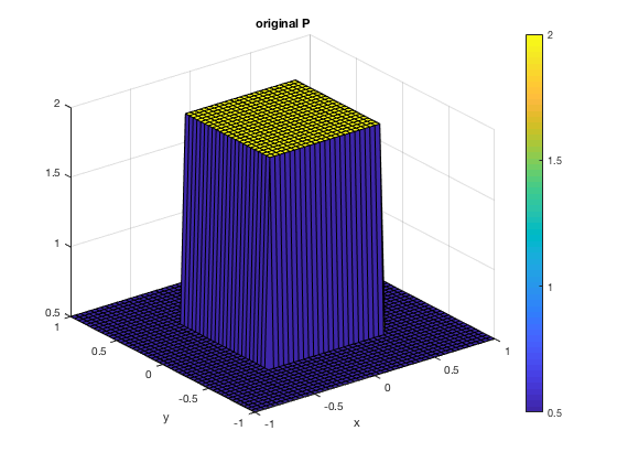
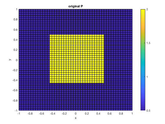
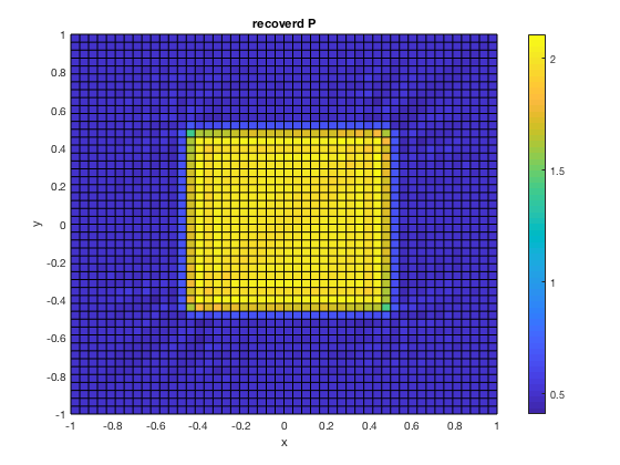
In the first example we assumed the parameter $P$ defined as, in [2],

(29) $$P_{1}(x,y)=\begin{cases}2,&\mbox{ if }|x|<0.5\mbox{ and }|y|<0.5\\ 0,&\mbox{ otherwise},\end{cases}$$

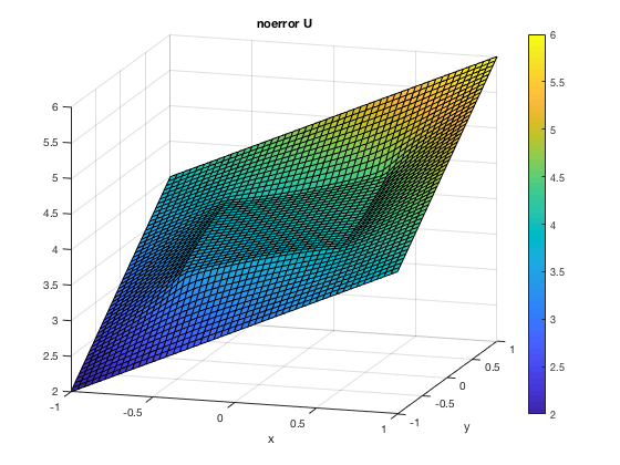
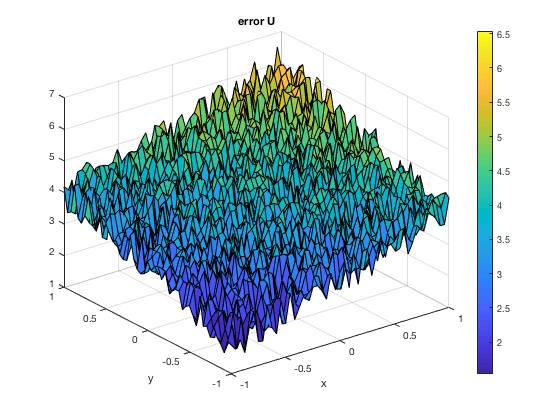
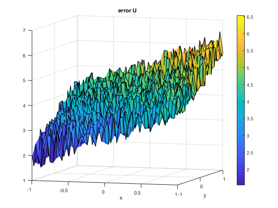
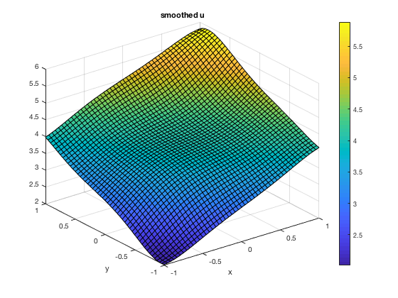
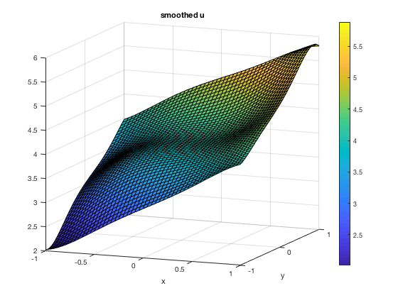
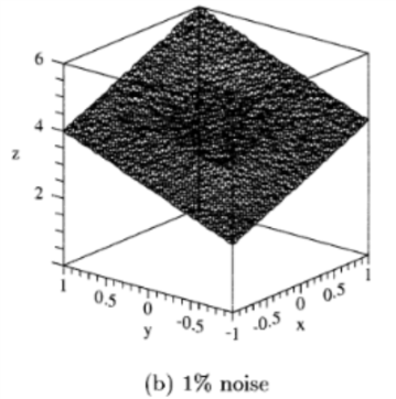
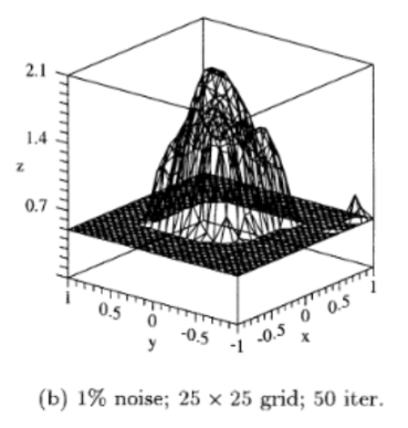
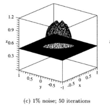
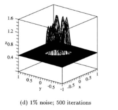
and the noisy free test data $u$ is constructed by solving (5) with the boundary function $\phi(x,y)=x+y+4$ on $\partial\Omega$. We then contaminate the data $u$ with uniform error to get $u_{\delta}$ such that the relative error $\frac{\lvert\lvert u-u_{\delta}\rvert\rvert_{\mathcal{L}^{1}}}{\lvert\lvert u\rvert\rvert_{\mathcal{L}^{1}}}\approx 7\%$. Figure 1 shows the true $u$, the noisy $u_{\delta}$ and the smoothed $\tilde{u}$, which is obtained from fitting a degree five two-dimensional polynomial through $u_{\delta}$, respectively. Notice that the information present in true $u$ is completely lost in the presence of noise (which is kind of extreme in this case) and, though smoothing (with a degree five polynomial) lead to some resemblance with the true $u$, it misses the key features. Nevertheless, the recovery, as seen in Figure 1, is still quite impressive. The parameter $P$ is recovered through minimizing the functional $G_{T}$, as defined in (27), and using the Dirichlet Neuberger gradient $\nabla_{\mathcal{H}^{1}}G$, as defined in (1.3). The relative error in the recovered $\tilde{P}$ is $\frac{\lvert\lvert P-\tilde{P}\rvert\rvert_{\mathcal{L}^{1}}}{\lvert\lvert P\rvert\rvert_{\mathcal{L}^{1}}}\approx 13.42\%$. We compare our results with the results obtained in [2], which is shown in Figure 3.

(a) True $u$

(b) True $u$

(c) noisy $u_{\delta}$

(d) noisy $u_{\delta}$

(e) smoothed $u$

(f) smoothed $u$

Figure 1. True $u$, noisy $u_{\delta}$ and smoothed $u$, for Example 2.

(a) True $P$

(b) True $P$

(c) Recovered $\tilde{P}$

(d) Recovered $\tilde{P}$

Figure 2. True $P$ and recovered $\tilde{P}$, for Example 2.

(a) $1\%$ error in the solution $u$

(b) 25 iterations, in a $25\times 25$ grid

(c) 50 iterations, $49\times 49$ grid

(d) 500 iterations, $49\times 49$ grid

Figure 3. Recovery of $P$ from [2] with $1\%$ error, for Example 2.

Remark 2.1.

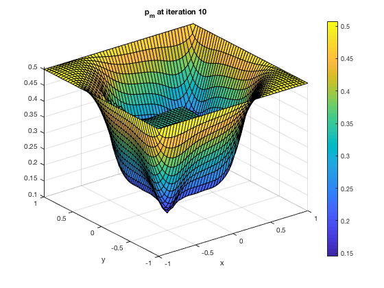
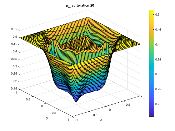
Note that, as mentioned previously, in this regularization method we didn’t specify a lower bound for the $P$ descent, i.e., the only constraint during the minimization process is, for all $m$, $p_{m}|_{\partial\Omega}=P|_{\partial\Omega}$ (for the uniqueness) and not on the lower bound for $p_{m}$’s, where as in [2] one has to have two constraints: (1) $p_{m}|_{\partial\Omega}=P|_{\partial\Omega}$ as well as $p_{m}\geq\nu>0$, for some constant $\nu$, otherwise the numerical solver crashes. We can see in Figure 4 the initial tendency of $p_{m}$ towards the negative values (rather than towards the unboundedness), which is the direct manifestation of the ill-posedness in the problem. In [2], the remedy implemented to handle this instability is to declare a cut-off value (0.5) for the functions $p_{m}$, below which the values of the descent iterates are reset to the cut-off value. With this modification, the algorithm became very stable (for noise-free $u$), allowing a steady descent to the minimum, and essentially no instabilities, even after thousands iterations. However, with this new regularization method we see that stability is embedded in the process, i.e., one doesn’t have to declare an external cut-off value to stabilize the process, it is self-restored (even in the case of noisy $u_{\delta}$).

(a) $p_{m}$ at iteration 10.

(b) $p_{m}$ at iteration 20.

(c) $p_{m}$ at iteration 50.

(d) $p_{m}$ at iteration 500.

(e) $p_{m}$ at iteration 1000.

(f) $p_{m}$ at iteration 2000.

Figure 4. $p_{m}$’s at different iterations, reflecting the stability of the process, for Example 2.

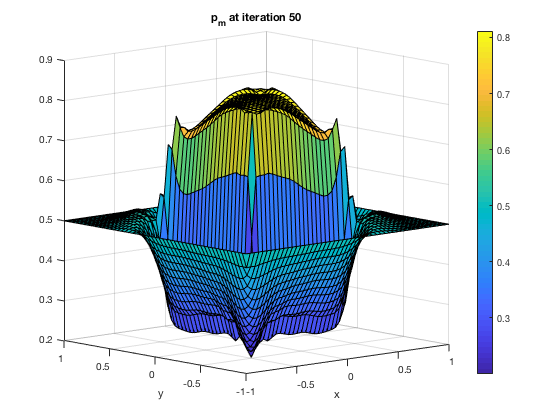
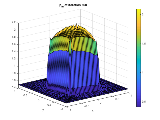
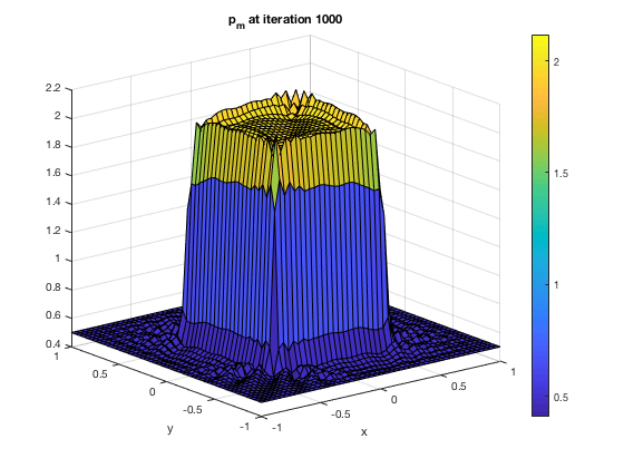
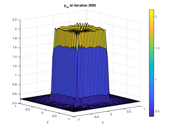
The next few examples deal with the parameter $P$ having both the negative as well as the positive values, i.e., not satisfying the condition (7), but $P(x)\neq 0$ on a set of non-zero measure.

Example 3.

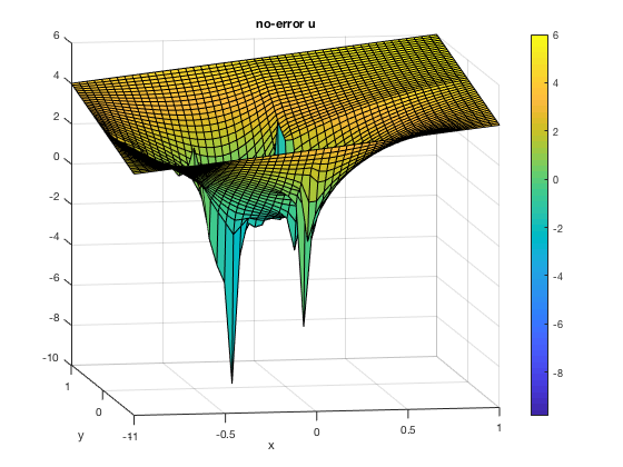
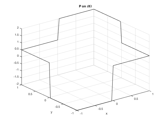
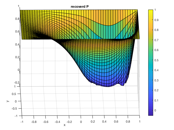
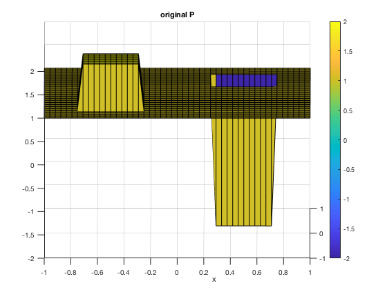
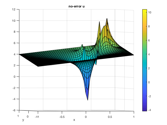
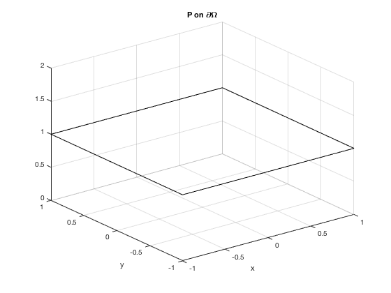
In this example, first, we consider a no-noise situation, i.e., $u=u_{\delta}$ or $\delta=0$. We consider the same domain $\Omega=[-1,1]\times[-1,1]$, discretized into $49\times 49$ evenly spaced grid, and the same boundary condition $\phi(x,y)=x+y+4$ on $\partial\Omega$, but the parameter to be recovered here is $P(x,y)=1+\sin(2xy)+\cos(2xy)$. As can be seen in Figure 5(a), $P$ has both the positive and negative values (but is not zero on a set of non-zero measure) and Figure 6(b) shows (the given) $P|_{\partial\Omega}$ such that $p_{m}|_{\partial\Omega}=P|_{\partial\Omega}$, for all $m$. We don’t contaminate the data $u$ with any noise and perform the minimization. The recovered parameter is shown in Figure 6(b), with a relative error of 0.0033%.

(a) True $P$

(b) Recovered $\tilde{P}$

Figure 5. True $P$ and recovered $\tilde{P}$, for Example 3.

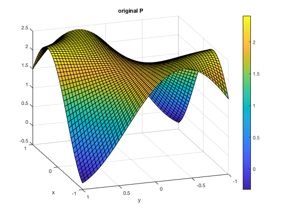
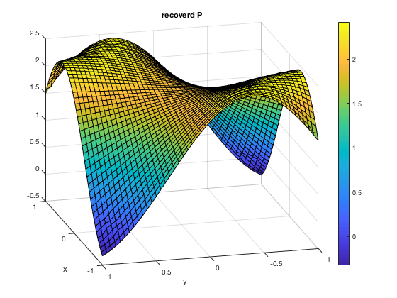
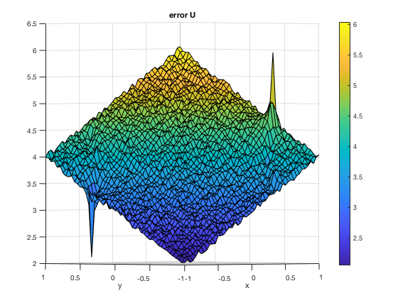
We repeat this example but this time with a noisy $u_{\delta}$, such that $\frac{\lvert\lvert u_{\delta}-u\rvert\rvert_{\mathcal{L}^{1}}}{\lvert\lvert u\rvert\rvert_{\mathcal{L}^{1}}}\approx 0.74\%$. The reason for such small error is due to the presence of two spikes in computed $u$, see Figure 7(a), which is a result of the presence of positive and negative values in $P$ and hence, a large error would have lead to losing of the spikes. Also note that in this case one can not use a polynomial surface-fit, as it will again lose the spikes. In this case we simply fit a surface ($\tilde{u_{\delta}}$), see Figure 7(b), generated by piecewise cubic interpolation, the disadvantage being, this leads to huge errors when estimating the $\nabla u$ using $\nabla\tilde{u_{\delta}}$ and also, one also has to be very careful when computing $T_{u_{\delta}}(p_{m})=-\nabla\cdot(p_{m}\nabla\tilde{u_{\delta}})$. Anyway, after carefully handling all of the above concerns, the recovered $P$ is shown in Figure 6(a), where the relative error in the recovery is around 25.57%.

(a) Recovered $\tilde{P}$, for Example 3.

(b) $P$ on $\partial\Omega$ for Example 3.

Figure 6. $P$ on the boundary $\partial\Omega$.

(a) noisy $u_{\delta}$.

(b) smoothed $\tilde{u_{\delta}}$

Figure 7. Noisy and smoothed data for Example 3

Example 4.

Here we consider another example of positive and negative $P$, which is defined on $\Omega$ as

(30) $$P(x,y)=\begin{cases}-2,\;\;&\mbox{ if }|x|<0\;\;\mbox{ and }|y|<0\\ 0.5,\;\;&\mbox{ if }|x|\geq 0\;\;\mbox{ and }|y|<0\\ 0.5,\;\;&\mbox{ if }|x|<0\;\;\mbox{ and }|y|\geq 0\\ 2,\;\;&\mbox{ if }|x|\geq 0\;\;\mbox{ and }|y|\geq 0.\end{cases}{}$$

The choice of the above $P$ increased the complexity of the computed solution in manifold ways, see Figure 9(a). Hence, we do not add any external noise in this example, i.e., $u_{\delta}=u$. The recovered $P$, with a relative error of 40%, is shown in Figure 8, and the constraint $p_{m}|_{\partial\Omega}=P|_{\partial\Omega}$ for the minimization is shown in Figure 9(b)

(a) Recovered $\tilde{P}$, for Example 4.

(b) True $P$ for Example 4.

Figure 8. True and recovered $P$ for Example 4.

(a) No-error $u$ for Example 4.

(b) $P$ on $\partial\Omega$ for Example 4.

Figure 9.   $u$ and $P|_{\partial\Omega}$ for Example 4.

Example 5.

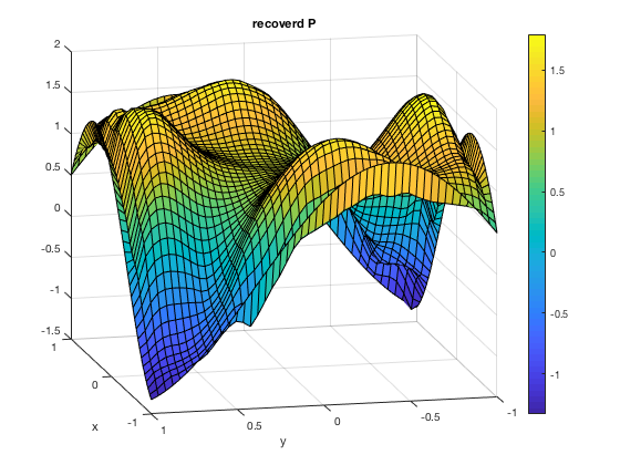
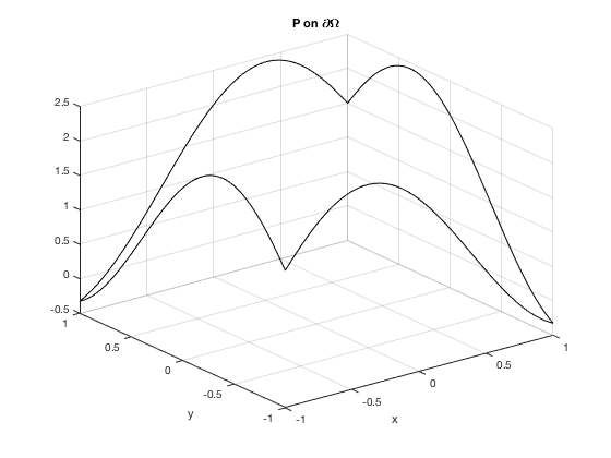
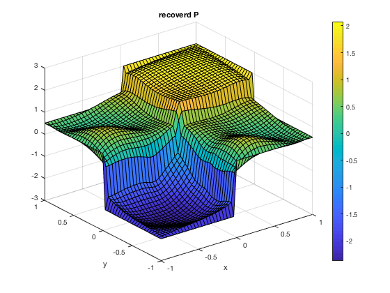
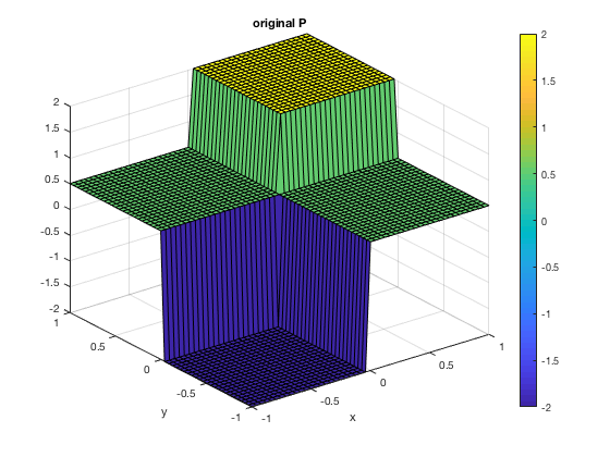
In the final example we demonstrate the importance of the boundary information. As seen in the Figures 6(b) and 9(b), the boundary data $P|_{\partial\Omega}$ does provide us the information that the parameter $P$ has both the positive and negative values. In this example we choose a $P$ which has both the negative and positive values, but the boundary data $P|_{\partial\Omega}$ doesn’t reflect it, i.e., $P$ is positive and negative in a strictly interior region $\Omega^{\prime}\subsetneq\Omega\backslash\partial\Omega$. The parameter $P$ is defined as

(31) $$P(x,y)=\begin{cases}-2,\;\;&\mbox{ if }-0.25<|x|<0.75\;\;\mbox{ and }-0.25<|y|<0.75\\ 2,\;\;&\mbox{ if }0.25<|x|<0.75\;\;\mbox{ and }0.25<|y|<0.75\\ 1,\;\;&\mbox{ otherwise}.\end{cases}{}$$

So one can observe that, from Figures 10(b) or 11(b), $P|_{\partial\Omega}$ does not contain any information regarding the negativity of $P$. Again, since the computed $u$, see Figure 11(a), has a complex structure we do not impose additional noise to it. Figure 10(a) shows the recovered $\tilde{P}$, with a relative error of 65.22% (after 704 iterations), and Figure 11(b) shows boundary data $P|_{\partial\Omega}$. Note that, as mentioned above, the recovery is unstable for $p_{m}=0$ on a set of non-zero measure and hence, the descent process is extremely slow when $p_{m}$ approaches 0 from the positive side, in an attempt to cross over to the negative side; where as in the previous examples (Example 3 and 4), since $p_{m}|_{\partial\Omega}=P|_{\partial\Omega}$ has both the positive and negative values, $p_{m}|_{p_{m}>0}\rightarrow P|_{P>0}$ and $p_{m}|_{p_{m}<0}\rightarrow P|_{P<0}$ (weakly) in $\mathcal{L}^{2}(\Omega)$.

(a) Recovered $\tilde{P}$, for Example 5.

(b) True $P$ for Example 5.

Figure 10.   True and recovered $P$ for Example 5.

(a) No-error $u$ for Example 5.

(b) $P$ on $\partial\Omega$ for Example 5.

Figure 11.   $u$ and $P|_{\partial\Omega}$ for Example 5.

Remark 2.2.

As we can see that, using the developed regularization method, the recovery of the parameter $P$ is very efficient even in the presence of extreme errors or when $P$ does not satisfy (7). Though we were not able to efficiently estimate $\nabla u_{\delta}$, still the method was very stable and quite effective. Hence, we expect to have even better results if we can extend the numerical differentiation procedure, developed for the single variable in Chapter $??$, to the multi-variable scenario. The other area of interest is to handle the case when the boundary data $P|_{\partial\Omega}$ does not contain any information about the parameter $P$ having both the positive and negative values. One may make use of the solution $u$ in that case, since the solution has peaks if $P$ has both positive and negative values.

References

- [1] I. Knowles and A. Yan, “The reconstruction of groundwater parameters from head data in an unconfined aquifer,” J. Comput. Appl. Math., vol. 208, no. 1, pp. 72–81, 2007.
- [2] I. Knowles, “Parameter identification for elliptic problems,” J. Comput. Appl. Math., vol. 131, no. 1-2, pp. 175–194, 2001.
- [3] I. Knowles and A. Yan, “On the recovery of transport parameters in groundwater modelling,” J. Comput. Appl. Math., vol. 171, no. 1-2, pp. 277–290, 2004.
- [4] I. Knowles, T. Le, and A. Yan, “On the recovery of multiple flow parameters from transient head data,” J. Comput. Appl. Math., vol. 169, no. 1, pp. 1–15, 2004.
- [5] I. Knowles and A. Yan, “The recovery of an anisotropic conductivity in groundwater modelling,” Appl. Anal., vol. 81, no. 6, pp. 1347–1365, 2002.
- [6] D. Gilbarg and N. S. Trudinger, Elliptic partial differential equations of second order. Springer-Verlag, Berlin-New York, 1977. Grundlehren der Mathematischen Wissenschaften, Vol. 224.
- [7] I. Knowles, “Uniqueness for an elliptic inverse problem,” SIAM J. Appl. Math., vol. 59, no. 4, pp. 1356–1370, 1999.
- [8] I. Knowles, “Coefficient identification in elliptic differential equations,” in Direct and inverse problems of mathematical physics (Newark, DE, 1997), vol. 5 of Int. Soc. Anal. Appl. Comput., pp. 149–160, Kluwer Acad. Publ., Dordrecht, 2000.
- [9] I. Knowles and M. A. LaRussa, “Conditional well-posedness for an elliptic inverse problem,” SIAM J. Appl. Math., vol. 71, no. 4, pp. 952–971, 2011.
- [10] J. W. Neuberger, Sobolev gradients and differential equations, vol. 1670 of Lecture Notes in Mathematics. Springer-Verlag, Berlin, 1997.