Near-Optimal Glimpse Sequences for Improved
Hard Attention Neural Network Training

Abstract

Hard visual attention is a promising approach to reduce the computational burden of modern computer vision methodologies. Hard attention mechanisms are typically non-differentiable. They can be trained with reinforcement learning but the high-variance training this entails hinders more widespread application. We show how hard attention for image classification can be framed as a Bayesian optimal experimental design (BOED) problem. From this perspective, the optimal locations to attend to are those which provide the greatest expected reduction in the entropy of the classification distribution. We introduce methodology from the BOED literature to approximate this optimal behaviour, and use it to generate ‘near-optimal’ sequences of attention locations. We then show how to use such sequences to partially supervise, and therefore speed up, the training of a hard attention mechanism. Although generating these sequences is computationally expensive, they can be reused by any other networks later trained on the same task.

1 Introduction

Attention can be defined as the “allocation of limited cognitive processing resources” [1]. In humans the density of photoreceptors varies across the retina. It is much greater in the centre [2] and covers an approximately 210 degree field of view [3]. This means that the visual system is a limited resource with respect to observing the environment and that it must be allocated, or controlled, by some attention mechanism. We refer to this kind of controlled allocation of limited sensor resources as “hard” attention. This is in contrast with “soft” attention, the controlled application of limited computational resources to full sensory input. Our focus in this paper is on hard attention mechanisms. Their foremost advantage is the ability to solve certain tasks using orders of magnitude less sensor bandwidth and computation than the alternatives [4, 5].

This paper focuses on the application of hard attention in image classification. Our model of attention (shown in Fig. 1) is as follows: a recurrent neural network (RNN) is given $T$ steps to classify some unchanging input image. Before each step, the RNN outputs the coordinates of a pixel in the image. A patch of the image centered around this pixel is then fed into the RNN. We call this image patch a glimpse, and the coordinates a glimpse location. As such, the RNN controls its input by selecting each glimpse location, and this decision can be based on previous glimpses. After $T$ steps, the RNN’s hidden state is mapped to a classification output. As with most artificial hard attention mechanisms [6, 7], this output is not differentiable with respect to the sequence of glimpse locations selected. This makes training with standard gradient backpropagation impossible, and so high variance gradient estimators such as REINFORCE [8] are commonly used instead [6, 7]. The resulting noisy gradient estimates make training difficult, especially for large $T$.

In order to improve hard attention training, we take inspiration from neuroscience literature which suggests that visual attention is directed so as to maximally reduce entropy in an agent’s world model [9, 10, 11, 12]. There is a corresponding mathematical formulation of such an objective, namely Bayesian optimal experimental design (BOED) [13, 14]. BOED tackles the problem of designing an experiment to maximally reduce uncertainty in some unknown variable. In the case of hard visual attention, the ‘experiment’ is the process of taking a glimpse; the ‘design’ is the glimpse location; and the unknown variable is the class label. In general, BOED is applicable only when a probabilistic model of the experiment exists. This could be, for example, a prior distribution over the class label and a generative model for the observed image patch conditioned on the class label and glimpse location. We leverage generative adversarial networks (GANs) [15, 16, 17] to provide such a model.

We use methodology from BOED to introduce the following training procedure for hard attention networks, which we call partial supervision by near-optimal glimpse sequences (PS-NOGS).

1. We assume that we are given an image classification task and a corresponding labelled dataset. Then, for some subset of the training images, we determine an approximately optimal (in the BOED sense) glimpse location for a hard attention network to attend to at each time step. We refer to the resulting sequences of glimpse locations as near-optimal glimpse sequences. Section 4 describes our novel method to generate them.

2. We use these near-optimal glimpse sequences to give an additional supervision signal for training a hard attention network. We introduce our novel training objective for this in Section 5, which utilises training images both with and without such sequences.

We empirically investigate the performance of PS-NOGS and find that it speeds up training compared to our baselines, and leads to qualitatively different behaviour with competitive accuracy. We also validate the use of BOED to generate the glimpse sequences by showing that even partial supervision by hand-crafted glimpse sequences does not have such a beneficial effect on training.

Figure 1: The hard attention network architecture we consider, consisting of an RNN core (yellow), a location network (light blue), a glimpse embedder (dark blue), and a classifier (red). $h_{t}$ is the RNN hidden state after $t$ steps. The network outputs distributions over where to attend ($l_{t}$) at each time step, and over the class label ($\theta$) after $T$ steps.

2 Hard attention

Given an image, $\mathcal{I}$, we consider the task of inferring its label, $\theta$. We use an architecture based on that of Mnih et al. [6], shown in Fig. 1. It runs for a fixed number of steps, $T$. At each step $t$, the RNN samples a glimpse location, $l_{t}$, which is conditioned on the previous glimpses via the RNN’s hidden state. A glimpse, in the form of a contiguous square of pixels, is extracted from the image at this location. We denote this $\mathbf{y}_{t}=f_{\text{fovea}}(\mathcal{I},l_{t})$. An embedding of $\mathbf{y}_{t}$ and $l_{t}$ is then input to the RNN. After $T$ glimpses, the network outputs a classification distribution $q_{\phi}(\theta|\mathbf{y}_{1:T},l_{1:T})$, where $\phi$ are the learnable network parameters. Mnih et al. [6] use glimpses consisting of three image patches at different resolutions, but the architectures are otherwise identical.

During optimisation, gradients cannot be computed by simple backpropagation since $f_{\text{fovea}}$ is non-differentiable. An alternative, taken by Mnih et al. [6] and others in the literature [7, 18], is to obtain high-variance gradient estimates using REINFORCE [8]. Although these are unbiased, their high-variance has made scaling beyond simple problems such as digit classification [19] challenging. Much research has focused on altering the architecture to ease the learning task: for example, many process the full, or downsampled, image before selecting glimpse locations [7, 18, 4, 20]. We summarise these innovations in Section 7 but note that they tend to be less suitable for low-power computation. We therefore believe that improved training of the architecture in Fig. 1 is an important research problem, and it is the focus of this paper.

3 Bayesian optimal experimental design

Designing an experiment to be maximally informative is a fundamental problem that applies as much to tuning the parameters of a political survey [21] as to deciding where to direct attention to answer a query. BOED [13] provides a unifying framework for this by allowing a formal comparison of possible experiments under problem-specific prior knowledge. Consider selecting the design, $l$, of an experiment to infer some unknown parameter, $\theta$. For example, $\theta$ may be the median lethal dose of a drug, and $l$ the doses of this drug given to various groups of rats [13]. Alternatively, as we consider in this paper, $\theta$ is the class label of an image and $l$ determines which part of the image we observe. The experiment results in a measurement of $\mathbf{y}\sim p(\mathbf{y}|l,\theta)$. For example, $\mathbf{y}$ could be the number of rats which die in each group or the observed pixel values. Given a prior distribution over $\theta$ and knowledge of $p(\mathbf{y}|l,\theta)$, we can use the measurement to infer a posterior distribution over $\theta$ using Bayes’ rule: $p(\theta|\mathbf{y},l)=\frac{p(\mathbf{y}|l,\theta)p(\theta)}{\int p(\mathbf{y}|l,\theta)p(\theta)\mathrm{d}\theta}$.

Figure 2: A near-optimal glimpse sequence being generated for the task of inferring the attribute ‘Male’. Top row: A heatmap of estimated expected posterior entropy for each possible next glimpse location $l_{t}$. The red cross marks the minimum, which is chosen as the next glimpse location. Bottom row: Observed parts of the image after taking each glimpse.

The aim of our experiment is to infer $\theta$, and so a well designed experiment will reduce the uncertainty about $\theta$ by as much as possible. The uncertainty after the experiment can be quantified by the Shannon entropy in the posterior:

$$\mathcal{H}\left[p(\theta|\mathbf{y},l)\right]=\mathbb{E}_{p(\theta|\mathbf{y},l)}\left[-\log p(\theta|\mathbf{y},l)\right].$$ (1)

To maximally reduce the uncertainty, we wish to select $l$ to minimise this posterior entropy. However, the design of the experiment must be chosen before $\mathbf{y}$ is measured and so we cannot evaluate the posterior entropy exactly. Instead, we minimise an expectation of it over $p(\mathbf{y}|l)=\mathbb{E}_{p(\theta)}\left[p(\mathbf{y}|l,\theta)\right]$, the marginal distribution of $\mathbf{y}$. This is the expected posterior entropy, or EPE:

$$\text{EPE}(l) =\mathbb{E}_{p(\mathbf{y}|l)}\left[\mathcal{H}\left[p(\theta|\mathbf{y},l)\right]\right].$$ (2)

Above, we considered the case of selecting a one-off design for an experiment, such as taking a single glimpse. For the case where a sequence of glimpses can be taken, we need sequential experimental design. In this scenario, the choice of design $l_{t}$ can be informed by the designs and outcomes of previous experiments, $l_{1:t-1}$ and $\mathbf{y}_{1:t-1}$. The marginal distribution over outcomes is therefore $p(\mathbf{y}_{t}|l_{1:t},\mathbf{y}_{1:t-1})$ rather than $p(\mathbf{y}_{t}|l_{t})$. Similarly, the posterior after observing $\mathbf{y}_{t}$ is $p(\theta|l_{1:t},\mathbf{y}_{1:t})$. Therefore, in the sequential case which we consider throughout the rest of the paper, we minimise the following form of the EPE:

$$\text{EPE}_{\mathbf{y}_{1:t-1},l_{1:t-1}}(l_{t})=\mathbb{E}_{p(\mathbf{y}_{t}|\mathbf{y}_{1:t-1},l_{1:t})}\left[\mathcal{H}\left[p(\theta|\mathbf{y}_{1:t},l_{1:t})\right]\right].$$ (3)

To summarise, sequential BOED involves, at each time $t$, selecting $l_{t}=\mathop{\rm arg\,min}_{l_{t}}\text{EPE}_{\mathbf{y}_{1:t-1},l_{1:t-1}}(l_{t})$ and then performing the experiment with design $l_{t}$ to observe $\mathbf{y}_{t}$.

4 Generating near-optimal glimpse sequences

Role of BOED pipeline   To reiterate the outline of our method, we first annotate a portion of the training data with glimpse sequences, and then in the second stage use these to speed up the training of a hard attention mechanism. This section details our BOED pipeline for the first stage.

EPE estimator   BOED requires a probabilistic model of the measurements and parameters we wish to infer. That is, we need to define $p(\theta,\mathbf{y}_{1:t}|l_{1:t})$ for any $l_{1:t}$. To do so in the visual attention setting, we first define $p(\theta,\mathcal{I})$ to be the intractable joint distribution over labels and images from which our training and test data originate. To be consistent with our definition in Section 2 of $\mathbf{y}$ as a deterministic function of $\mathcal{I}$ and $l$, we then define $p(\mathbf{y}_{i}|\mathcal{I},l_{i})$ to be a Dirac-delta distribution on $f_{\text{fovea}}(\mathcal{I},l_{i})$. The joint distribution is then

$$p(\theta,\mathbf{y}_{1:t}|l_{1:t})=\int p(\theta,\mathcal{I})\prod_{i=1}^{t}p(\mathbf{y}_{i}|\mathcal{I},l_{i})\mathrm{d}\mathcal{I}.$$ (4)

Given this joint distribution, $\text{EPE}_{\mathbf{y}_{1:t-1},l_{1:t-1}}(l_{t})$ is well defined but intractable in general. We therefore consider how to approximate it. To simplify our method for doing do, we first rearrange the expression given in eq. 3 so that the expectation is over $\mathcal{I}$ rather than $\mathbf{y}_{t}$. Taking advantage of the fact that $\mathbf{y}_{i}$ is a deterministic function of $\mathcal{I}$ and $l_{i}$ allows it to be rewritten as follows (proof in the appendix). Defining $f_{\text{fovea}}(\mathcal{I},l_{1:t})=\{f_{\text{fovea}}(\mathcal{I},l_{1}),\ldots,f_{\text{fovea}}(\mathcal{I},l_{t})\}$,

$$\text{EPE}_{\mathbf{y}_{1:t-1},l_{1:t-1}}(l_{t})=\mathbb{E}_{p(\mathcal{I}|\mathbf{y}_{1:t-1},l_{1:t-1})}\left[\mathcal{H}\left[p(\theta|f_{\text{fovea}}(\mathcal{I},l_{1:t}),l_{1:t})\right]\right].$$ (5)

Given this form of the expected posterior entropy, we can approximate it if we can leverage the dataset to make the following two approximations:

• a learned attentional variational posterior, ${g_{\text{AVP}}}(\theta|\mathbf{y}_{1:t},l_{1:t})\approx p(\theta|\mathbf{y}_{1:t},l_{1:t})$,

• and stochastic image completion distribution ${r_{\text{img}}}(\mathcal{I}|\mathbf{y}_{1:t-1},l_{1:t-1})\approx p(\mathcal{I}|\mathbf{y}_{1:t-1},l_{1:t-1})$.

We expand on the form of each of these approximations later in this section. First, combining them with eq. 5 and using a Monte Carlo estimate of the expectation yields our estimator for the EPE:

$$\text{EPE}_{\mathbf{y}_{1:t-1},l_{1:t-1}}\left(l_{t}\right)\approx\frac{1}{N}\sum_{n=1}^{N}\mathcal{H}\big{[}{g_{\text{AVP}}}(\theta|f_{\text{fovea}}(\mathcal{I}^{(n)},l_{1:t}),l_{1:t})\big{]}$$ (6)

with $\mathcal{I}^{(1)}\ldots,\mathcal{I}^{(N)}\sim{r_{\text{img}}}(\mathcal{I}|\mathbf{y}_{1:t-1},l_{1:t-1})$.

Overview of BOED pipeline   We select $l_{t}$ with a grid search. That is, denoting the set of allowed values of $l_{t}$ as $L$, we compute our approximation of $\text{EPE}_{\mathbf{y}_{1:t-1},l_{1:t-1}}(l_{t})$ for all $l_{t}\in L$. We then select the value of $l_{t}$ for which this is least. To do so, our full BOED pipeline is as follows.

1. Sample $\mathcal{I}^{(1)}\ldots,\mathcal{I}^{(N)}\sim{r_{\text{img}}}(\mathcal{I}|\mathbf{y}_{1:t-1},l_{1:t-1})$.

2. For each $l_{t}\in L$, approximate the expected posterior entropy with eq. 6.

3. Select the value of $l_{t}$ for which this approximation is least.

This is repeated for each $t=1,\ldots,T$. Figure 2 shows examples of EPEs estimated in this way for each $t$. We now detail the form of ${g_{\text{AVP}}}$ (the attentional variational posterior) and ${r_{\text{img}}}$ (stochastic image completion).

Figure 3: Attentional variational posterior CNN. An RGB image and $l_{1:t}$ are processed to create an embedding of the information gained from glimpses $1$ to $t$. This embedding is fed into an image classifier to obtain an approximation of $p(\theta|\mathbf{y}_{1:t},l_{1:t})$.

Attentional variational posterior   In this section we introduce our novel approach to efficiently approximating the intractable posterior $p(\theta|\mathbf{y}_{1:t},l_{1:t})$. We train a convolutional neural network (CNN) to map from a sequence of glimpses , $\mathbf{y}_{1:t}$, and their locations, $l_{1:t}$, to ${g_{\text{AVP}}}(\theta|\mathbf{y}_{1:t},l_{1:t})$, an approximation of this posterior. We call this the attentional variational posterior CNN (AVP-CNN). To allow a single CNN to cope with varying $\mathbf{y}_{1:t}$, $l_{1:t}$, and even varying $t$, we embed its input as shown in Fig. 3. Essentially, $l_{1:t}$ is used to create a mask the size of the image which is 1 for observed pixels and 0 for unobserved pixels. Elementwise multiplication of this mask with the input image sets unobserved pixels to zero. The mask is then concatenated as an additional channel. This embedding naturally maintains spatial information while enforcing an invariance to permutations of the glimpse sequence. Our experiments use a Densenet-121 [22] CNN architecture (pretrained on ImageNet [23]) to map from this embedding to a vector of class probabilities representing ${g_{\text{AVP}}}$.

We train the network to minimise the KL divergence between its output and $p(\theta|\mathbf{y}_{1:t},l_{1:t})$. That is, $D_{KL}\left(p(\theta|\mathbf{y}_{1:t},l_{1:t})||{g_{\text{AVP}}}(\theta|\mathbf{y}_{1:t},l_{1:t})\right)$. To ensure that ${g_{\text{AVP}}}$ is close for all $t$, $l_{1:t}$ and $\mathbf{y}_{1:t}$, the loss used is an expectation of this KL divergence over $p(\mathbf{y}_{1:t}|l_{1:t})u(t,l_{1:t})$. We factorise $u(t,l_{1:t})$ as $u(t)\prod_{i=1}^{t}u(l_{i})$ where, so that all times and glimpse locations are weighted equally in the loss, $u(t)$ is a uniform distribution over $1,\ldots,T$ and $u(l_{i})$ is a uniform distribution over all image locations. Denoting the network parameters $\lambda$, the gradient of this loss is

$$\frac{\partial}{\partial\lambda}\mathcal{L}_{\lambda}=\mathbb{E}_{p(\theta,\mathbf{y}_{1:t}|l_{1:t})u(t,l_{1:t})}\left[-\frac{\partial}{\partial\lambda}\log g_{\text{AVP}}^{\lambda}(\theta|\mathbf{y}_{1:t},l_{1:t})\right].$$ (7)

This gradient is the same as that of a cross-entropy loss on data sampled from $p(\theta,\mathbf{y}_{1:t}|l_{1:t})u(t,l_{1:t})$, and can be approximated by a Monte Carlo estimate.

Our approximation of the EPE in eq. 6 involves the entropy of ${g_{\text{AVP}}}$. Since ${g_{\text{AVP}}}$ is a categorical distribution, this is simple to compute analytically. Our approximation of the posterior entropy by an amortised artifact in this way is inspired by the variational posterior estimator introduced by Foster et al. [14], although there are two important differences:

• Foster et al. learn a mapping from $\mathbf{y}_{t}$ to $g(\theta|\mathbf{y}_{1:t},l_{1:t})$, sharing information between “nearby” samples of $\mathbf{y}_{t}$ to reduce the computational cost of the experimental design. Our AVP-CNN takes this amortization further by learning a single mapping from $t$, $l_{1:t}$ and $\mathbf{y}_{1:t}$ to ${g_{\text{AVP}}}(\theta|\mathbf{y}_{1:t},l_{1:t})$, which yields significant further efficiency gains in our setting.

• Whereas we approximate $\mathcal{H}[p]$ with $\mathcal{H}[{g_{\text{AVP}}}]=\mathbb{E}_{g_{\text{AVP}}}[-\log{g_{\text{AVP}}}]$, Foster et al. use $\mathbb{E}_{p}[-\log g]$. This provides an upper bound on $\mathcal{H}[p]$ but is not applicable in our case as we cannot sample from $p(\theta|\mathbf{y}_{1:t},l_{1:t})$. Both approximations are exact when ${g_{\text{AVP}}}=p$.

Stochastic image completion   We considered numerous ways to form ${r_{\text{img}}}(\mathcal{I}|\mathbf{y}_{1:t-1},l_{1:t-1})$ including inpainting techniques [24, 25] and through Markov chain Monte Carlo in a probabilistic image model. Future research in GANs and generative modelling may provide better alternatives to this component of our method but, for now, we choose to represent ${r_{\text{img}}}$ using a technique we developed based on image retrieval [26]. We found that, of the methods we considered, this gives the best trade-off between speed and sample quality. It involved creating an empirical image distribution consisting of 1.5 million images for each experiment using deep generative models with publicly available pre-trained weights (StyleGAN [16] for CelebA-HQ and FineGAN [17] for Caltech-UCSD Birds). During sampling, the database is searched for images that ‘match’ the previous glimpses ($\mathbf{y}_{1:t-1}$ and $l_{1:t-1}$). How well these glimpses match some image in the database, $\mathcal{I}^{\prime}$, is measured by the squared distance in pixel space at glimpse locations: $\sum_{i=1}^{t-1}\left\lVert\mathbf{y}_{i}-f_{\text{fovea}}(\mathcal{I}^{\prime},l_{i})\right\rVert^{2}_{2}$. This distance is used to define a probability distribution over the images in the database. To reduce computation, we first cheaply compare approximations of the observed parts of each image using principal component analysis [27], and compute exact distances only when these are close. The overall procedure to sample from ${r_{\text{img}}}$ corresponds to importance sampling [28] in a probabilistic model where $p(\mathbf{y}_{t}|\mathcal{I},l_{t})$ is relaxed from a Dirac-delta distribution to a Gaussian. See the appendix for further details.

5 Training with partial supervision

The previous section describes how to annotate an image with a near-optimal sequence of glimpse locations for a particular image classification task. This section assumes that these, or other forms of glimpse sequence (e.g. the handcrafted glimpse sequences in Section 6), exist for all, or some, images in a dataset. These can then be used to partially supervise the training of a hard attention mechanism on this dataset. We refer to glimpse sequences used in this way as supervision sequences. We use separate losses for supervised (i.e. annotated with both a class label and a sequence of glimpse locations) and unsupervised (i.e. annotated with a class label but not glimpse locations) examples. By minimising the sum of these losses, our procedure can be viewed as maximising the joint log-likelihood of the class labels and supervision sequences. To be precise, let $q_{\phi}(\theta^{i},l_{1:T}^{i}|\mathcal{I}^{i})$ be a network’s joint distribution over the chosen glimpse locations and predicted class label on image $\mathcal{I}^{i}$. Let $q_{\phi}(\theta^{i}|\mathcal{I}^{i})$ be the marginalisation of this distribution over $l^{i}_{1:t}$. We maximise a lower bound on

$$\mathbf{L}=\sum_{i\in\text{sup.}}\overbrace{\log q_{\phi}(\theta^{i},l_{1:T}^{i}|\mathcal{I}^{i})}^{\text{supervised objective}}+\sum_{i\in\text{unsup.}}\overbrace{\log q_{\phi}(\theta^{i}|\mathcal{I}^{i})}^{\text{unsupervised objective}}.$$ (8)

where ‘sup’ is the set of training indices with supervision sequences, and ‘unsup’ is the remainder.

When running on unsupervised examples, we follow Mnih et al. [6] and train the location network with a REINFORCE estimate of the gradient of the accuracy, using a learned baseline to reduce the variance of this estimate. Meanwhile, the RNN, glimpse embedder, and classifier network are trained to maximise the log-likelihood of the class labels (i.e. minimise a cross-entropy loss). Ba et al. [7] noted that this can be viewed as maximising a lower bound on the unsupervised objective in eq. 8. For examples with supervision sequences, the supervised objective in eq. 8 is maximised by gradient backpropagation. The loss is computed by running the network with its glimpse locations fixed to those in the supervision sequence. The location network is updated to maximise the probability of outputting these glimpse locations while, as for unsupervised examples, the other network modules are trained to maximise the likelihood of the class labels. Gradients of the supervised and unsupervised objectives can be computed simultaneously, with minibatches containing both types of example.

Figure 4: Comparison of glimpse locations chosen by RAM and PS-NOGS on the CelebA-HQ test set for three classification tasks. For each $t\in\{1,2,3,4,5\}$, we show an image where each pixel’s colour corresponds to how often it was observed at this time step during testing. The outlines are produced by averaging outputs from a face detector across the dataset. For $t=1$, each network learns a single location which it attends to on every test image. This is expected behaviour as the first location is chosen before taking any glimpses, and therefore before being able to condition on the image. RAM appears to then fail to learn to direct the later glimpses, attending almost uniformly across the image. In contrast, PS-NOGS distributes these glimpses broadly over the salient regions.

6 Experiments and results

Datasets and network architectures   We test our approach on CelebA-HQ [29] and a cropped variant of Caltech-UCSD Birds (CUB) [30], both of which are convincingly modelled by state-of-the-art GANs [16, 17] as we require. For both datasets, we use $T=5$. The hard attention network’s classifier is a fully-connected layer mapping from the hidden state to a softmax output and the location network has a single 32-dimensional hidden layer. All hard attention networks are trained by Adam optimiser [31] with a batch size of 64; learning rate $3\times 10^{-4}$ for CelebA-HQ and $5\times 10^{-5}$ for CUB; and other hyperparameters set to the recommended defaults [31]. The dataset-specific details are as follows: (1) CelebA-HQ Our experiments tackle 40 different binary classification tasks, corresponding to the 40 labelled attributes. We resize the images to $224\times 224$ and use training, validation, and test sets of $27\,000$, $500$, and $2500$ images respectively. We use $16\times 16$ pixel glimpses, with a $50\times 50$ grid of allowed glimpse locations. The glimpse network has two convolutional layers followed by a linear layer, and the RNN is a GRU [32] with hidden dimension $64$. (2) CUB We perform 200-way classification of bird species. We crop the images using the provided bounding boxes and resize them to $128\times 128$. Cropping is necessary because good generative models do not exist for the uncropped dataset, but there is still considerable variation in pose after cropping. We use 5120 training images, a validation set of 874 and a test set of 5751 (having removed 43 images also found in ImageNet). We use $32\times 32$ pixel glimpses and a $12\times 12$ grid of allowed glimpse locations so that adjacent locations are 8 pixels apart. The glimpse network is the first 12 convolutional layers of a VGG pretrained on ImageNet [33, 23], and the RNN is a GRU with hidden dimension $1024$.

Figure 5: Number of training iterations for each CelebA-HQ attribute before a validation cross-entropy loss within 0.01 of the best is achieved. On average, PS-NOGS trains almost $7\times$ faster than RAM and with less than a fifth of the variance in training speed. This speed-up is complemented by an average increase in test accuracy of $0.4\%$. Attributes are sorted by RAM’s mean training time.

BOED   We create $600$ near-optimal glimpse sequences for each of the 40 CelebA-HQ classification tasks, and $1000$ for CUB. This took approximately 20 GPU-hours for CUB, and 10 GPU days for each CelebA-HQ attribute. We have publicly released these sequences along with our code, allowing them to be re-used by anyone to speed up the training of hard attention networks on these tasks.

RAM baseline   On both experiments, we train our architecture with the algorithm used for the recurrent attention model (RAM) of Mnih et al. [6] as a baseline, which is equivalent to the special case of our partially supervised objective with zero supervision sequences. We compare this to our method of partially-supervising training using near-optimal glimpse sequences (PS-NOGS).

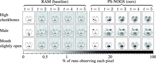
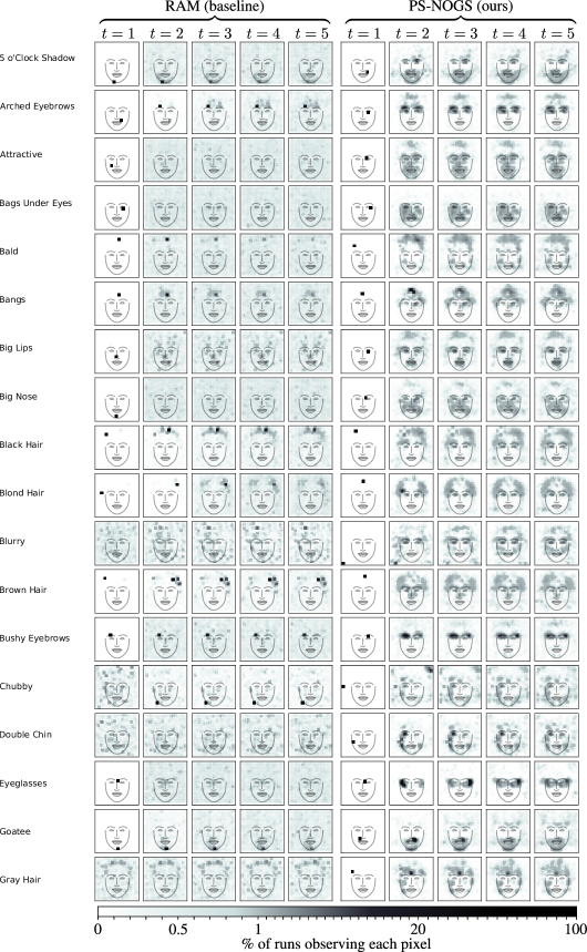
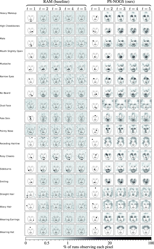
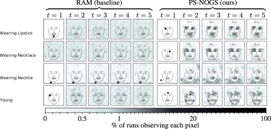
Partial-supervision for CelebA-HQ   In Fig. 5, we plot the number of iterations until convergence for RAM and PS-NOGS on each different CelebA-HQ classification task. Using PS-NOGS reduced the average number of iterations by a factor of 6.8 compared to RAM ($3500$ vs. $24\,000$) while improving mean test accuracy from $86.7\%$ to $87.1\%$. We also compare the attention policies learned by each method. These are plotted for several tasks in Fig. 4, and for the remainder in the appendix. RAM has difficulty learning policies for more than the first glimpse. PS-NOGS appears to learn a reasonable policy for every timestep.

Figure 6: CUB validation accuracy over training.

Partial-supervision for CUB   For experiments on CUB, we find that a pretraining stage is required to obtain good final classification accuracy. We therefore pretrain the classifier, RNN, and glimpse network with glimpse locations sampled independently at each time step from either a uniform distribution (in the case of RAM) or from a heuristic which assigns higher probability to more salient locations, as estimated using the AVP-CNN (RAM+ and all others). Additional details are available in the appendix. We train both RAM baselines and PS-NOGS. We also consider partial supervision with hand-crafted glimpse sequences, PS-HGS. The hand-crafted glimpse sequences are designed, using CUB’s hand-annotated features, to always attend to the beak, eye, forehead, belly and feet (in that order). If any of these parts are obscured, they are replaced by a randomly selected visible body part.

Table 1: Results summary

	CelebA-HQ (avg.)		CUB
Method	Iterations	Accuracy (%)	Iterations	Accuracy (%)
RAM / RAM+	24 000	86.7	11 600	56.3
PS-HGS	-	-	960	52.0
PS-NOGS (ours)	3500	87.1	640	55.4

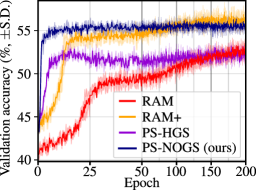
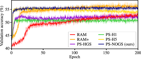
In Figure 6, we plot the validation accuracy of the various methods throughout training. We find that PS-NOGS outperforms the baselines at the start of training, achieving $54\%$ accuracy after just 5 epochs. In comparison, the RAM+ model takes 16 epochs to reach $54\%$ and PS-HGS never does. The naive baseline RAM has worse validation accuracy throughout training than RAM+, which uses the AVP-CNN for pre-training. Finally, we note that after  95 epochs, the validation accuracy for RAM+ overtakes that for PS-NOGS. This may be because REINFORCE has unbiased gradient estimates, whereas error due to approximations in the generation of supervision sequences leads to a bias throughout training. Table 1 summarises the accuracy and iterations until convergence on each dataset, with the best technique on each metric in bold. The number of iterations on CUB is the number before achieving a validation accuracy within 1% of the highest.

7 Related work

Hard attention architectures   Elsayed et al. [20] recently demonstrated a hard attention network which achieved accuracy on ImageNet [23] close to that of CNNs which use the whole image. However, their approach neccesitates running a convolutional network on the entire image to select glimpse locations. As such, they advertise improvements in interpretability rather than computational efficiency. Sermanet et al. [18] train a hard attention architecture with REINFORCE to achieve state-of-the-art accuracy on the Stanford Dogs dataset. In addition to accessing the full image in low resolution at the start, they use large glimpses (multiple $96\times 96$ pixel patches at different resolutions) to effectively solve the task in a single step. This avoids problems resulting from learning long sequences with REINFORCE but also rules out the computational gains possible with smaller glimpses. Katharopoulos and Fleuret [4] proposed a form of hard attention where, after processing the downsampled image, multiple glimpses are sampled and processed simultaneuosly. This is again incompatible with a low-power setting where we cannot afford to operate on the full image.

Supervised attention   One solution to improving training is to provide supervision targets for the attention mechanism. This is common in visual question answering, usually for training soft attention. Typically the targets are created by human subjects, either with gaze-tracking [34] or explicit data annotation [35]. Either way is expensive and dataset-specific [35, 36]. Recent work has considered reducing this cost by, for example, extrapolating supervision signals from a manually-annotated dataset to other, related, datasets [37], or using existing segmentations to speed up annotation [36]. Even so, considerable human effort is required. Our method for generating near-optimal glimpse sequences can be viewed as automation of this in an image classification context.

8 Discussion and conclusion

We have demonstrated a novel BOED pipeline for generating near-optimal sequences of glimpse locations. We also introduced a partially supervised training objective which uses such a supervision signal to speed up the training of a hard attention mechanism. By investing up-front computation in creating near-optimal glimpse sequences for supervision, this speed up can be achieved along with comparable final accuracy. Since we release the near-optimal glimpse sequences we generated, faster training and experimentation on these tasks is available to the public without the cost of generating new sequences. Our work could also have applications in neural architecture search, where this cost can be amortised over many training runs with different architectures.

There is potential to significantly speed up the BOED pipeline by, for example, selecting $l_{t}$ though Bayesian optimisation rather than a grid search. Our framework could also be extended to attention tasks such as question answering where the latent variable of interest is richly structured.

Broader Impact

Our work on hard attention aims to make possible more power-efficient computer vision. This could make certain computer vision methods more feasible in settings where limited power is available, such as in embedded devices, or for applications with extremely large data throughput, such as processing satellite images. These applications can have a positive impact through, for example, environmental monitoring or healthcare but also potential negative implications, particularly with regard to privacy. We hope that standards and legislation can be developed to mitigate these concerns.

Another motivation for hard visual attention is its interpretability [20, 38], since a network’s outputs can be more easily understood if we know which part of the image informed them. This is especially applicable to the hard attention architecture considered in our work, which never accesses the full image. Greater traction for such architectures, whether motivated by power efficiency or interpretability, would therefore lead to computer vision systems making more interpretable decisions. This may lead to more trust being placed in such systems. An important research direction is the implications of this trust, and whether it is justified by this level of interpretability.

Appendix A Details for method

A.1 BOED pseudocode

Algorithm 1 gives pseudocode for our BOED pipeline. This selects a near-optimal glimpse location for a single timestep. Repeating this for $t=1,\ldots,T$ yields a near-optimal glimpse sequence for a particular image. Figure 7 provides a visualisation of the various stages of this algorithm.

1:procedure SelectLocation($\mathbf{y}_{1:t-1},l_{1:t-1}$)

2:     $\mathcal{I}^{(1)},\ldots,\mathcal{I}^{(N)}\sim r_{\text{img}}(\mathcal{I}|\mathbf{y}_{1:t-1},l_{1:t-1})$ $\triangleright$ stochastic image completion

3:     for $l_{t}\in L$ do $\triangleright$ grid search for $l_{t}$

4:         for $n\leftarrow 1,\ldots,N$ do

5:              $\text{PE}_{l_{t}}^{(n)}\leftarrow\mathcal{H}\left[{g_{\text{AVP}}}(\theta|f_{\text{fovea}}(\mathcal{I}^{(n)},l_{1:t}),l_{1:t})\right]$ $\triangleright$ estimate posterior entropy

6:         end for

7:         $\text{EPE}_{l_{t}}\leftarrow\frac{1}{N}\sum_{n=1}^{N}\text{PE}_{l_{t}}^{(n)}$ $\triangleright$ average over Monte Carlo samples

8:     end for

9:     $l_{t}^{*}\leftarrow\mathrm{argmin}_{l_{t}}\text{EPE}_{l_{t}}$

10:     return $l_{t}^{*}$

11:end procedure

Algorithm 1 BOED pipeline to select $l_{t}$. This roughly follows the three-step procedure given in Section 4: $N$ images are sampled in line 2; these are used to estimate expected posterior entropies for each $l_{t}\in L$ in lines 3-7. Finally, the minimising value of $l_{t}$ is found on line 9.

.

Figure 7: BOED procedure to select $l_{2}$ given $\mathbf{y}_{1}$ and $l_{1}$, corresponding to algorithm 1 with $t=2$. Panel 1 shows a visualisation of the single previous glimpse, $\mathbf{y}_{1}$, taken at $l_{1}$, with all unobserved image pixels displayed in pink. Panel 2 shows $\mathcal{I}^{(1)},\ldots,\mathcal{I}^{(N)}$, Monte Carlo samples of the full image drawn on line 2 of algorithm 1. For each of these images, panel 3 shows a heatmap. Each heatmap plots the estimated posterior entropy after conditioning on $\mathbf{y}_{t}=f_{\text{fovea}}(\mathcal{I},l^{*})$ and $l_{t}=l^{*}$ for each $l^{*}\in L$, plotted against the $x$ and $y$ coordinates of $l^{*}$. These posterior entropies are estimated on line 5, and then averaged over the Monte Carlo samples on line 7, giving the expected posterior entropies displayed by a heatmap in panel 4. Finally, $l_{t}$ is chosen to minimise $\text{EPE}_{l_{t}}$.

A.2 EIG estimator in eq. 5

This section derives the form of the expected posterior entropy presented in eq. 5. Starting from eq. 3, we introduce an inner expectation over $\mathcal{I}$:

$$\text{EPE}_{\mathbf{y}_{1:t-1},l_{1:t-1}}(l_{t}) =\mathbb{E}_{p(\mathbf{y}_{t}|\mathbf{y}_{1:t-1},l_{1:t})}\left[\mathcal{H}\left[p(\theta|\mathbf{y}_{1:t},l_{1:t})\right]\right]$$ (9)

$$=\mathbb{E}_{p(\mathbf{y}_{t}|\mathbf{y}_{1:t-1},l_{1:t})}\mathbb{E}_{p(\mathcal{I}|\mathbf{y}_{1:t},l_{1:t})}\left[\mathcal{H}\left[p(\theta|\mathbf{y}_{1:t},l_{1:t})\right]\right]$$ (10)

$$=\mathbb{E}_{p(\mathbf{y}_{t},\mathcal{I}|\mathbf{y}_{1:t-1},l_{1:t})}\left[\mathcal{H}\left[p(\theta|\mathbf{y}_{1:t},l_{1:t})\right]\right].$$ (11)

Since, according to the probabilistic model defined in eq. 4, each $\mathbf{y}_{i}$ is a deterministic function of $\mathcal{I}$ and $l_{i}$ we can substitute $\mathbf{y}_{1:t}$ using the definition $\mathbf{y}_{1:t}=f_{\text{fovea}}(\mathcal{I},l_{1:t})=\{f_{\text{fovea}}(\mathcal{I},l_{1}),\ldots,f_{\text{fovea}}(\mathcal{I},l_{t})\}$.

$$\text{EPE}_{\mathbf{y}_{1:t-1},l_{1:t-1}}(l_{t}) =\mathbb{E}_{p(\mathbf{y}_{t},\mathcal{I}|\mathbf{y}_{1:t-1},l_{1:t})}\left[\mathcal{H}\left[p(\theta|f_{\text{fovea}}(\mathcal{I},l_{1:t}),l_{1:t})\right]\right]$$ (12)

$$=\mathbb{E}_{p(\mathcal{I}|\mathbf{y}_{1:t-1},l_{1:t-1})}\left[\mathcal{H}\left[p(\theta|f_{\text{fovea}}(\mathcal{I},l_{1:t}),l_{1:t})\right]\right]$$ (13)

as presented in eq. 5.

A.3 Stochastic image completion

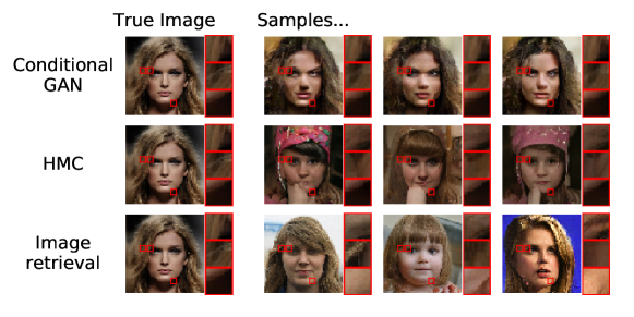
This section provides more detail on our method for stochastic image completion and the alternatives we considered, as discussed in Section 4. Three sampling mechanisms for ${r_{\text{img}}}(\mathcal{I}|\mathbf{y}_{1:t-1},l_{1:t-1})$ were compared qualitatively, based on both the diversity of samples produced and how realistic the samples are (taking into account the previous observations). These were a conditional GAN, HMC in a deep generative model, and the image retrieval-based approach used in our pipeline. We now provide more detail on each.

A.3.1 Conditional GAN

We considered a conditional GAN, motivated by recent state-of-the-art performance on conditional image generation problems [39, 24]. In particular, we considered using pix2pix [25] to map from an embedding of $\mathbf{y}_{1:t}$ and $l_{1:t}$ (similar to that in Fig. 3 but without concatenating the mask, and with unobserved pixels replaced with Gaussian noise instead of zeros) to the completed image. We used the U-net architecture [40] with resolution $256\times 256$. Fig. 8 shows samples when all other hyperparameters were set to the defaults [25]. We tried varying both the generator architecture and the weight given to the L1-norm, although neither significantly improved the quality of the generated images. Although the GAN can learn to generate realistic images for CelebA-HQ, they have very little diversity when the observations are fixed. An additional issue is that the outputs looked considerably less realistic for the Caltech-UCSD birds dataset.

A.3.2 HMC in a deep generative model

We also considered taking a pre-existing, unconditional, GAN (StyleGAN [16]) with publicly available weights and using Hamiltonian Monte Carlo [41, 42] (HMC) to sample images from it conditioned on the observations. Specifically, we sample from $p(\mathcal{I}|\mathbf{y}_{1:t},l_{1:t})\propto p(\mathcal{I})\prod_{i=1}^{t}p(\mathbf{y}_{i}|\mathcal{I},l_{i})$, where $p(\mathcal{I})$ is the prior over images defined by the GAN. Deviating from the model specified in eq. 4, we define $p(\mathbf{y}_{i}|\mathcal{I},l_{i})$ to be an isotropic Gaussian centred on $f_{\text{fovea}}(\mathcal{I},l_{i})$, rather than a Dirac-delta on $f_{\text{fovea}}(\mathcal{I},l_{i})$. This change is necessary to make inference with HMC feasible. We used an implementation of HMC in Pyro [43], a probabilistic programming language. Samples are shown in the second row of Fig. 8. These were taken using a likelihood with standard deviation 0.4 applied to the normalised pixel values, which was set to trade-off the ‘closeness’ of samples to the true image and the feasibility of inference. The integration was performed with 200 steps of size 0.05 and all other parameters set to the defaults. Although the samples mostly look realistic, they suffered from low sample diversity; the HMC chains became stuck in certain modes and did not explore the full posterior. Additionally, sampling was slow: drawing each sample took approximately a minute on a GPU.

Figure 8: Sampled image completions using various techniques. The glimpse locations are marked with red squares, and close-ups of each glimpse are shown to the right of each image. The leftmost column shows the ‘true’ image from which the observed glimpses are taken and the others show samples conditioned on these glimpses.

A.3.3 Image retrieval

Algorithm 2 SampleImages calls SampleProposal to select $K_{1}$ images to load into memory, based on approximations of their importance weights. These are then reweighted using their exact likelihood. $K_{2}$ images are sampled from the resulting weighted categorical distribution, and returned.

procedure SampleProposal($\mathcal{I},l_{1:t}$)

     Select relevant weight matrix columns $\mathbf{\tilde{W}}\leftarrow\textsc{Slice}(\mathbf{W},l_{1:t})$

     Select relevant columns of mean vector $\mathbf{\tilde{\mu}}\leftarrow\textsc{Slice}(\mathbf{\mu},l_{1:t})$

     Reconstruct observations $\mathbf{\hat{y}}_{1:t}\leftarrow\mathbf{\tilde{\mu}}+\mathbf{\tilde{W}}^{\top}\mathbf{W}\mathcal{I}$

     for $i=1,\ldots,{N^{\text{data}}}{}$ do

         Approximate observed patches $\mathbf{\hat{y}}_{1:t}^{i}\leftarrow\mathbf{\tilde{W}}^{\top}\mathbf{z}^{i}$

         Compute approximate likelihood $w^{i}_{1}\leftarrow\mathcal{N}\left(\mathbf{\hat{y}}_{1:t}|\mathbf{\hat{y}}_{1:t}^{i},\sigma_{q}^{2}\right)$

     end for

     $j^{(1)},\ldots,j^{(K_{1})}\leftarrow\textsc{Resample}(w^{1}_{1},\ldots,w_{1}^{N^{\text{data}}}{})$

     return $\{i^{(k)},w_{1}^{i^{(k)}}\}\text{ for }k=1,\ldots,K_{1}$

end procedure

procedure SampleImages($\mathcal{I},l_{1:t}$)

     Input: $\mathcal{I},l_{1:t}$

     $\{i^{(1)},w^{i^{(1)}}_{1}\},\ldots,\{i^{(K_{1})},w^{i^{(K_{1})}}_{1}\}=\textsc{SampleProposal}(\mathcal{I},l_{1:t})$

     for $k=1,\ldots,K_{1}$ do

         Load $\mathcal{I}^{i^{(k)}}$

         $\mathbf{y}^{k}_{1:t}\leftarrow\text{Glimpse}(\mathcal{I}^{i^{(k)}},l_{1:t})$

         Compute exact likelihood $p(\mathbf{y}_{1:t}|\mathcal{I}^{i^{(k)}},l_{1:t})=\mathcal{N}\left(\mathbf{y}_{1:t}|\mathbf{y}_{1:t}^{k},\sigma_{p}^{2}\right)$

         Compute weight $w^{(k)}_{2}\leftarrow\frac{p(\mathbf{y}_{1:t}|\mathcal{I}^{i^{(k)}},l_{1:t})}{w^{i^{(k)}}_{1}}$

     end for

     $j^{(1)},\ldots,j^{(K_{2})}\leftarrow\textsc{Resample}(w^{1}_{2},\ldots,w^{K_{1}}_{2})$

     return $\mathcal{I}^{j^{(k)}}\text{ for }k=1,\ldots,K_{2}$

end procedure

Our stochastic image retrieval procedure proceeds as follows. We begin with a large dataset of images $\mathcal{I}^{1},\ldots,\mathcal{I}^{N^{\text{data}}}{}$ independently sampled from $p(\mathcal{I})$ (or an approximation of it). We are then given some observations, $\mathbf{y}_{1:t},l_{1:t}$ and, roughly speaking, want to approximate $K_{2}$ samples from $p(\mathcal{I}|\mathbf{y}_{1:t},l_{1:t})$ using $K_{2}$ images from the dataset. We begin by assigning each image $i$ in the dataset a weight, $w_{1}^{i}$, which approximates the likelihood $p(\mathbf{y}_{1:t}|\mathcal{I}^{i},l_{1:t})$. This approximation is efficiently computed using PCA, as we describe later. We then construct a categorical proposal distribution over these images, where the probability of each is proportional to the weight. We draw $K_{1}$ samples from this proposal. These images are then retrieved from the database. To make up for the inexact weights computed previously, we reweight these samples using exact likelihoods. These weights are used to compute a categorical distribution over the $K_{1}$ images. This distribution approximates $p(\mathcal{I}|\mathbf{y}_{1:t},l_{1:t})$ increasingly well as ${N^{\text{data}}}{}$ (the dataset size) and $K_{1}$ tend to infinity. $K_{2}$ samples from this distribution are returned.

Principal component analysis allows for a memory-efficient representation of the dataset through a mean image, $\mathbf{\mu}$, a low-dimensional vector for each image, $\mathbf{z}^{i}$, and an orthogonal matrix, $\mathbf{W}$, which transforms from an image, $\mathcal{I}^{i}$, into the corresponding $\mathbf{z}^{i}$ as follows:

$$\mathbf{z}^{i}=\mathbf{W}\mathcal{I}^{i}$$ (14)

Denoting the dimensionality of $\mathbf{z}$ as $L$, the number of images as ${N^{\text{data}}}{}$, and the number of pixels per image as $P$, these objects can be stored with memory complexity $\Theta({N^{\text{data}}}{}L+PL)$, compared to $\Theta({N^{\text{data}}}{}P)$ for the entire dataset. Since $\mathbf{W}$ is orthogonal, image $i$ can be approximated using $\mathbf{z}^{i}$ as

$$\mathbf{\hat{x}}^{i}=\mathbf{W}^{\top}\mathbf{z}^{i}$$ (15)

and $\mathbf{\hat{x}}\approx\mathcal{I}$ for large enough $L$. If only certain pixels of the reconstructed image are required, $\mathcal{I}^{i}_{p_{1}:p_{C}}$ these can be obtained efficiently by using $\mathbf{\tilde{W}}^{\top}$, a matrix made up of rows $p_{1}$ to $p_{C}$ of $\mathbf{W}^{\top}$:

$$\mathcal{I}^{i}_{p_{1}:p_{C}}=\mathbf{\tilde{W}}^{\top}\mathbf{z}^{i}.$$ (16)

This allows us to construct an approximation of the observed portion with each image in the dataset in a time and memory-efficient manner. Additionally, we found that our proposal was improved when the approximate likelihood was calculated with a reconstruction of the observations as $\mathbf{\hat{y}}_{1:t}=\mathbf{\tilde{W}}^{\top}\mathbf{W}\mathcal{I}$, rather than the true observations $\mathbf{y}_{1:t}$. Although this requires access to the full true image, this is acceptable as the full image was always available when we carried out our experimental design. Also, since this is only used to calculate the proposal distribution, it should have limited effect on the samples returned after new weights are calculated with the exact likelihood.

The algorithms we use in our experiments vary in the following ways from algorithm 2. They both expand the effective size of the generated dataset by comparing the observations with a horizontally-flipped version of each dataset image, as well as the original version. Additionally for CelebA-HQ, in order to increase the sample size and impose an invariance to very small translations, the likelihoods (for both the proposal and the exact likelihood) for each image are given by summing the Gaussian likelihoods over a grid of image patches taken at locations close to the observed location. For CUB, a simpler alteration is made to increase the effective sample size: $\sigma_{q}$ is tuned while creating each proposal distribution so that it will have an effective sample size roughly equal to the number of samples drawn. The attached code contains both variations.

Appendix B Experimental details

B.1 AVP-CNN training

Here, we expand on the training procedure for the AVP-CNN which was described in Section 4. For CelebA-HQ, it was trained to predict each of the 40 attributes simultaneously by outputting a vector parameterising an independent Bernoulli distribution for each, which we found to improve accuracy compared to training a network for each. Similarly for CUB, the AVP-CNN output a vector of probabilities for each of the 312 binary attributes in the dataset, in addition to the 200-dimensional categorical distribution. These outputs were produced by linear mappings (and a sigmoid/softmax) from the same final hidden layer. The predictions for the binary attributes of CUB were not used; this was done purely to improve the training of the classifier.

For both datasets, the AVP-CNN was initialised from weights pretrained on ImageNet, with only the final layer replaced and an additional input channel added (with weights initialised to zero). It was then trained using Adam optimizer with a learning rate of $1\times 10^{-4}$ and a batch size of 64. Validation was performed and a checkpoint saved every epoch, and the checkpoint which gave the lowest validation cross-entropy was used. This occurred after $183$ epochs for the network used to create near-optimal glimpse sequences on CUB and after $458$ for CelebA-HQ. For both datasets, the training set for the AVP-CNN was chosen to exclude the examples on which Bayesian experimental design was later performed in order to prevent any potential issues with using the AVP-CNN to approximate classification distributions on data which it may be overfitted to.

B.2 CUB pretraining

As mentioned in the paper, we found a pretraining stage to be important for achieving high accuracy on CUB. During this stage, the parameters of the RNN, glimpse embedder, and classifier were trained, while the location network was not used. After 250 epochs of pretraining, saved parameters from the epoch with highest validation accuracy were used for the next stage of training. These parameters were then frozen while the location network was trained. The only difference between our pretraining loss and our training loss is that pretraining glimpse locations are sampled from some fixed distribution, instead of from the distribution proposed by the location network. As mentioned in the paper, this is a uniform distribution over all $l_{t}\in L$ for RAM. We now describe the heuristic distribution used to pretrain the other networks. In all our tests, we found that this heuristic gave better performance than the uniform distribution.

The heuristic distribution uses $\text{EPE}_{\emptyset,\emptyset}(l)$ as a measure of the saliency of a location. That is, the expected entropy in the posterior after taking a single glimpse at $l$. Since this is not conditioned on any previous glimpses, it is independent of the image being processed. This is used to create a distribution over locations as:

$$\log p^{\text{loc}}(l)=C-\gamma^{-1}\cdot\text{EPE}_{\emptyset,\emptyset}(l)$$ (17)

where $\gamma^{-1}$ is the inverse temperature, which we set to $1$. $C=-\log\sum_{l}\exp\left(-\gamma^{-1}\cdot\text{EPE}_{\emptyset,\emptyset}(l)\right)$ is a constant chosen such that $p^{\text{loc}}$ is a normalised distribution. We estimate $\text{EPE}_{\emptyset,\emptyset}(l)$ for each $l$ using our BOED pipeline.

B.3 Additional baselines

In addition to the hand-crafted glimpse sequences described in Section 6, we here consider another form of heuristic supervision sequence as a baseline. These were created by sampling glimpse locations independently at each time step from the distribution defined in eq. 17. We ran experiments with both $\gamma^{-1}=1$ (denoted PS-H1) and $\gamma^{-1}=5$ (denoted PS-H5).

Figure 12 shows validation accuracy for these over the course of training. We find that networks trained with PS-H1 and PS-H5 converge quickly: after 240 and 400 iterations respectively, as measured by when they reach within 1% of the highest validation accuracy. This may be due to the simplicity of the policies that the supervision sequences encourage them to learn, with identical and independent distributions over the glimpse location at every time step. Despite their fast convergence, the validation accuracy for these heuristics appears to be almost always lower than that for PS-NOGS throughout training, and never higher by a statistically significant margin.

B.4 Architectural details

As mentioned, we use a learned baseline to reduce the variance of the REINFORCE gradient estimate. Following Mnih et al. [6], this is in the form of a linear ‘baseline’ network which maps from the RNN hidden state to a scalar estimate of the reward.

The glimpse embedder for CelebA-HQ consisted of the following, in order: a $3\times 3$ convolution to 16 channels with stride 1; a ReLU activation; a $3\times 3$ convolution to 32 channels with stride 2; a ReLU and $2\times 2$ max pool; and a linear layer mapping the output of this to the $64$-dimensional RNN input.

B.5 Hyperparameters

For the Monte Carlo estimation of the expected posterior entropy in eq. 6, we use $N=200$ Monte Carlo samples for CelebA-HQ and $N=100$ for CUB.

For the stochastic image completion algorithm, we use the following hyperparameters for CelebA-HQ: $K_{1}=1000$; $K_{2}=200$; and $\sigma_{p}=\sigma_{q}=5\times 2^{t}$ for each timestep $t$. For CUB, we use: $K_{1}=500$; $K_{2}=100$; $\sigma_{p}=80$; and a dynamically adjusted $\sigma_{q}$ (as descibed in section A.3.3). For both datasets, we use a 256-dimensional latent space for the PCA and ${N^{\text{data}}}=1\,500\,000$.

To allow direct comparison between PS-NOGS and the baseline supervision sequences (PS-HGS, PS-H1 and PS-H5), we supervise the same number of training images for each; that is, 600 for tasks on CelebA-HQ and 1000 for CUB classification.

Appendix C Additional plots

C.1 Glimpse locations

Building on Fig. 4 in the paper, Figures 9 to 11 show the glimpse locations of networks trained with each of RAM and PS-NOGS for all 40 CelebA-HQ attributes.

Figure 9: Glimpse locations on CelebA-HQ.

Figure 10: Glimpse locations on CelebA-HQ.

Figure 11: Glimpse locations on CelebA-HQ.

C.2 CUB training

Figure 12 shows the validation accuracy throughout training for CUB, including for the additional baselines from section B.3.

Figure 12: Expanded version of Fig. 6 including the additional baselines described in section B.3.

C.3 Supervision sequences

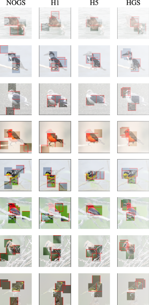
Figure 13 shows supervision glimpse sequences given by various methods. These are for a random sample of images.

Figure 13: Examples of the image areas observed by near-optimal glimpse sequences (NOGS); sequences generated using the heuristic described in section B.3 with $\gamma^{-1}=1$ (H1) or $\gamma^{-1}=5$ (H5); and hand-crafted glimpse sequences (HGS).

References

- Anderson [2005] John R Anderson. Cognitive psychology and its implications. Macmillan, 2005.
- Bear et al. [2007] Mark F Bear, Barry W Connors, and Michael A Paradiso. Neuroscience, volume 2. Lippincott Williams & Wilkins, 2007.
- Traquair [1949] Harry Moss Traquair. An introduction to clinical perimetry. Mosby, 1949.
- Katharopoulos and Fleuret [2019] Angelos Katharopoulos and Francois Fleuret. Processing megapixel images with deep attention-sampling models. In Kamalika Chaudhuri and Ruslan Salakhutdinov, editors, Proceedings of the 36th International Conference on Machine Learning, volume 97 of Proceedings of Machine Learning Research, pages 3282–3291, Long Beach, California, USA, 09–15 Jun 2019. PMLR. URL http://proceedings.mlr.press/v97/katharopoulos19a.html.
- Rensink [2000] Ronald A Rensink. The dynamic representation of scenes. Visual cognition, 7(1-3):17–42, 2000.
- Mnih et al. [2014] Volodymyr Mnih, Nicolas Heess, Alex Graves, et al. Recurrent models of visual attention. In Advances in neural information processing systems, pages 2204–2212, 2014.
- Ba et al. [2014] Jimmy Ba, Volodymyr Mnih, and Koray Kavukcuoglu. Multiple object recognition with visual attention. arXiv preprint arXiv:1412.7755, 2014.
- Williams [1992] Ronald J Williams. Simple statistical gradient-following algorithms for connectionist reinforcement learning. Machine learning, 8(3-4):229–256, 1992.
- Bruce and Tsotsos [2009] Neil DB Bruce and John K Tsotsos. Saliency, attention, and visual search: An information theoretic approach. Journal of vision, 9(3):5–5, 2009.
- Itti and Baldi [2009] Laurent Itti and Pierre Baldi. Bayesian surprise attracts human attention. Vision research, 49(10):1295–1306, 2009.
- Schwartenbeck et al. [2013] Philipp Schwartenbeck, Thomas FitzGerald, Ray Dolan, and Karl Friston. Exploration, novelty, surprise, and free energy minimization. Frontiers in psychology, 4:710, 2013.
- Feldman and Friston [2010] Harriet Feldman and Karl Friston. Attention, uncertainty, and free-energy. Frontiers in human neuroscience, 4:215, 2010.
- Chaloner and Verdinelli [1995] Kathryn Chaloner and Isabella Verdinelli. Bayesian experimental design: A review. Statistical Science, pages 273–304, 1995.
- Foster et al. [2019] Adam Foster, Martin Jankowiak, Eli Bingham, Paul Horsfall, Yee Whye Teh, Tom Rainforth, and Noah Goodman. Variational estimators for Bayesian optimal experimental design. arXiv preprint arXiv:1903.05480, 2019.
- Goodfellow et al. [2014] Ian Goodfellow, Jean Pouget-Abadie, Mehdi Mirza, Bing Xu, David Warde-Farley, Sherjil Ozair, Aaron Courville, and Yoshua Bengio. Generative adversarial nets. In Advances in neural information processing systems, pages 2672–2680, 2014.
- Karras et al. [2018] Tero Karras, Samuli Laine, and Timo Aila. A style-based generator architecture for generative adversarial networks. arXiv preprint arXiv:1812.04948, 2018.
- Singh et al. [2019] Krishna Kumar Singh, Utkarsh Ojha, and Yong Jae Lee. Finegan: Unsupervised hierarchical disentanglement for fine-grained object generation and discovery. In Proceedings of the IEEE Conference on Computer Vision and Pattern Recognition, pages 6490–6499, 2019.
- Sermanet et al. [2014] Pierre Sermanet, Andrea Frome, and Esteban Real. Attention for fine-grained categorization. arXiv preprint arXiv:1412.7054, 2014.
- Netzer et al. [2011] Yuval Netzer, Tao Wang, Adam Coates, Alessandro Bissacco, Bo Wu, and Andrew Y Ng. Reading digits in natural images with unsupervised feature learning. NIPS Workshop on Deep Learning and Unsupervised Feature Learning 2011, 2011.
- Elsayed et al. [2019] Gamaleldin F Elsayed, Simon Kornblith, and Quoc V Le. Saccader: Improving accuracy of hard attention models for vision. arXiv preprint arXiv:1908.07644, 2019.
- Warwick and Lininger [1975] Donald P Warwick and Charles A Lininger. The sample survey: Theory and practice. McGraw-Hill, 1975.
- Huang et al. [2017] Gao Huang, Zhuang Liu, Laurens Van Der Maaten, and Kilian Q Weinberger. Densely connected convolutional networks. In Proceedings of the IEEE conference on computer vision and pattern recognition, pages 4700–4708, 2017.
- Deng et al. [2009] J. Deng, W. Dong, R. Socher, L.-J. Li, K. Li, and L. Fei-Fei. ImageNet: A Large-Scale Hierarchical Image Database. In CVPR09, 2009.
- Pathak et al. [2016] Deepak Pathak, Philipp Krahenbuhl, Jeff Donahue, Trevor Darrell, and Alexei A Efros. Context encoders: Feature learning by inpainting. In Proceedings of the IEEE conference on computer vision and pattern recognition, pages 2536–2544, 2016.
- Isola et al. [2017] Phillip Isola, Jun-Yan Zhu, Tinghui Zhou, and Alexei A Efros. Image-to-image translation with conditional adversarial networks. In Proceedings of the IEEE conference on computer vision and pattern recognition, pages 1125–1134, 2017.
- Jégou et al. [2010] Hervé Jégou, Matthijs Douze, and Cordelia Schmid. Improving bag-of-features for large scale image search. International journal of computer vision, 87(3):316–336, 2010.
- Jolliffe [2011] Ian Jolliffe. Principal component analysis. Springer, 2011.
- Arulampalam et al. [2002] M Sanjeev Arulampalam, Simon Maskell, Neil Gordon, and Tim Clapp. A tutorial on particle filters for online nonlinear/non-Gaussian Bayesian tracking. IEEE Transactions on signal processing, 50(2):174–188, 2002.
- Karras et al. [2017] Tero Karras, Timo Aila, Samuli Laine, and Jaakko Lehtinen. Progressive growing of gans for improved quality, stability, and variation. arXiv preprint arXiv:1710.10196, 2017.
- Wah et al. [2011] C. Wah, S. Branson, P. Welinder, P. Perona, and S. Belongie. The Caltech-UCSD Birds-200-2011 Dataset. Technical Report CNS-TR-2011-001, California Institute of Technology, 2011.
- Kingma and Ba [2014] Diederik P Kingma and Jimmy Ba. Adam: A method for stochastic optimization. arXiv preprint arXiv:1412.6980, 2014.
- Cho et al. [2014] Kyunghyun Cho, Bart Van Merriënboer, Caglar Gulcehre, Dzmitry Bahdanau, Fethi Bougares, Holger Schwenk, and Yoshua Bengio. Learning phrase representations using RNN encoder-decoder for statistical machine translation. arXiv preprint arXiv:1406.1078, 2014.
- Simonyan and Zisserman [2014] Karen Simonyan and Andrew Zisserman. Very deep convolutional networks for large-scale image recognition. arXiv preprint arXiv:1409.1556, 2014.
- Yu et al. [2017] Youngjae Yu, Jongwook Choi, Yeonhwa Kim, Kyung Yoo, Sang-Hun Lee, and Gunhee Kim. Supervising neural attention models for video captioning by human gaze data. In Proceedings of the IEEE Conference on Computer Vision and Pattern Recognition, pages 490–498, 2017.
- Das et al. [2017] Abhishek Das, Harsh Agrawal, Larry Zitnick, Devi Parikh, and Dhruv Batra. Human attention in visual question answering: Do humans and deep networks look at the same regions? Computer Vision and Image Understanding, 163:90–100, 2017.
- Gan et al. [2017] Chuang Gan, Yandong Li, Haoxiang Li, Chen Sun, and Boqing Gong. VQS: Linking segmentations to questions and answers for supervised attention in VQA and question-focused semantic segmentation. In Proceedings of the IEEE International Conference on Computer Vision, pages 1811–1820, 2017.
- Qiao et al. [2018] Tingting Qiao, Jianfeng Dong, and Duanqing Xu. Exploring human-like attention supervision in visual question answering. In Thirty-Second AAAI Conference on Artificial Intelligence, 2018.
- Xu et al. [2015] Kelvin Xu, Jimmy Ba, Ryan Kiros, Kyunghyun Cho, Aaron Courville, Ruslan Salakhudinov, Rich Zemel, and Yoshua Bengio. Show, attend and tell: Neural image caption generation with visual attention. In International Conference on Machine Learning, pages 2048–2057, 2015.
- Nazeri et al. [2019] Kamyar Nazeri, Eric Ng, Tony Joseph, Faisal Qureshi, and Mehran Ebrahimi. Edgeconnect: Generative image inpainting with adversarial edge learning. arXiv preprint arXiv:1901.00212, 2019.
- Ronneberger et al. [2015] Olaf Ronneberger, Philipp Fischer, and Thomas Brox. U-net: Convolutional networks for biomedical image segmentation. In International Conference on Medical image computing and computer-assisted intervention, pages 234–241. Springer, 2015.
- Duane et al. [1987] Simon Duane, Anthony D Kennedy, Brian J Pendleton, and Duncan Roweth. Hybrid Monte Carlo. Physics letters B, 195(2):216–222, 1987.
- Hoffman and Gelman [2014] Matthew D Hoffman and Andrew Gelman. The No-U-Turn sampler: adaptively setting path lengths in Hamiltonian Monte Carlo. Journal of Machine Learning Research, 15(1):1593–1623, 2014.
- Bingham et al. [2018] Eli Bingham, Jonathan P. Chen, Martin Jankowiak, Fritz Obermeyer, Neeraj Pradhan, Theofanis Karaletsos, Rohit Singh, Paul Szerlip, Paul Horsfall, and Noah D. Goodman. Pyro: Deep universal probabilistic programming. arXiv preprint arXiv:1810.09538, 2018.