Kaskade: Graph Views for Efficient Graph Analytics
Abstract
Graphs are an increasingly popular way to model real-world entities and relationships between them, ranging from social networks to data lineage graphs and biological datasets. Queries over these large graphs often involve expensive sub-graph traversals and complex analytical computations. These real-world graphs are often substantially more structured than a generic vertex-and-edge model would suggest, but this insight has remained mostly unexplored by existing graph engines for graph query optimization purposes. Therefore, in this work, we focus on leveraging structural properties of graphs and queries to automatically derive materialized graph views that can dramatically speed up query evaluation.
We present Kaskade, the first graph query optimization framework to exploit materialized graph views for query optimization purposes. Kaskade employs a novel constraint-based view enumeration technique that mines constraints from query workloads and graph schemas, and injects them during view enumeration to significantly reduce the search space of views to be considered. Moreover, it introduces a graph view size estimator to pick the most beneficial views to materialize given a query set and to select the best query evaluation plan given a set of materialized views. We evaluate its performance over real-world graphs, including the provenance graph that we maintain at Microsoft to enable auditing, service analytics, and advanced system optimizations. Our results show that Kaskade substantially reduces the effective graph size and yields significant performance speedups (up to 50X), in some cases making otherwise intractable queries possible.
I Introduction
Many real-world applications can be naturally modeled as graphs, including social networks [1, 2], workflow, and dependency graphs as the ones in job scheduling and task execution systems [3, 4], knowledge graphs [5, 6], biological datasets, and road networks [7]. An increasingly relevant type of workload over these graphs involves analytics computations that mix traversals and computation, e.g., finding subgraphs with specific connectivity properties or computing various metrics over sub-graphs. This has resulted in a large number of systems being designed to handle complex queries over such graphs [8, 9].
In these scenarios, graph analytics queries require response times on the order of a few seconds to minutes, because they are either exploratory queries run by users (e.g., recommendation or similarity search queries) or they power systems making online operational decisions (e.g., data valuation queries to control replication, or job similarity queries to drive caching decisions). However, many of these queries involve the enumeration of large subgraphs of the input graph, which can easily take minutes to hours to compute over large graphs on modern graph systems. To achieve our target response times over large graphs, new techniques are needed.
We observe that the graphs in many of these applications have an inherent structure: their vertices and edges have specific types, following well-defined schemas and connectivity properties. For instance, social network data might include users, pages, and events, which can be connected only in specific ways (e.g., a page cannot “like” a user), or workload management systems might involve files and jobs, with all files being created or consumed by some job. As we discuss in § I-A, the provenance graph that we maintain at Microsoft has similar structural constraints. However, most existing graph query engines do not take advantage of this structure to improve query evaluation time.
At the same time, we notice that similar queries are often run repeatedly over the same graph. Such queries can be identified and materialized as views to avoid significant computation cost during their evaluation. The aforementioned structural regularity of these graphs can be exploited to efficiently and automatically derive these materialized views. Like their relational counterparts, such graph views allow us to answer queries by operating on much smaller amounts of data, hiding/amortizing computational costs and ultimately delivering substantial query performance improvements of up to 50X in our experiments on real-world graphs. As we show, the benefits of using graph views are more pronounced in heterogeneous graphs111By heterogeneous, we refer to graphs that have more than one vertex types, as opposed to homogeneous with a single vertex type. that include a large number of vertex and edge types with connectivity constraints between them.
I-A Motivating example

At Microsoft, we operate one of the largest data lakes worldwide, storing several exabytes of data and processing them with hundreds of thousands of jobs, spawning billions of tasks daily [10]. Operating such a massive infrastructure requires us to handle data governance and legal compliance (e.g., GDPR [11]), optimize our systems based on our query workloads, and support metadata management and enterprise search for the entire company, similar to the scenarios in [3, 4]. A natural way to represent this data and track datasets and computations at various levels of granularity is to build a provenance graph that captures data dependencies among jobs, tasks, files, file blocks, and users in the lake. As discussed above, only specific relationships among vertices are allowed, e.g., a user can submit a job, and a job can read or write files.
To enable these applications over the provenance graph, we need support for a wide range of structural queries. Finding files that contain data from a particular user or created by a particular job is an anchored graph traversal that computes the reachability graph from a set of source vertices, whereas detecting overlapping query sub-plans across jobs to avoid unnecessary computations can be achieved by searching for jobs with the same set of input data. Other queries include label propagation (i.e., marking privileged derivative data products), data valuation (i.e., quantifying the value of a dataset in terms of its “centrality” to jobs or users accessing them), copy detection (i.e., finding files that are stored multiple times by following copy jobs that have the same input dataset), and data recommendation (i.e., finding files accessed by other users who have accessed the same set of files that a user has).
We highlight the optimization opportunities in these types of queries through a running example: the job blast radius. Consider the following query operating on the provenance graph: “For every job , quantify the cost of failing it, in terms of the sum of CPU-hours of (affected) downstream consumers, i.e., jobs that directly or indirectly depend on ’s execution.” This query, visualized in Fig. 1, traverses the graph by following read/write relationships among jobs and files, and computes an aggregate along the traversals. Answering this query is necessary for cluster operators and analysts to quantify the impact of job failures—this may affect scheduling and operational decisions.
By analyzing the query patterns and the graph structure, we can optimize the job blast radius query in the following ways. First, observe that the graph has structural connectivity constraints: jobs produce and consume files, but there are no file-file or job-job edges. Second, not all vertices and edges in the graph are relevant to the query, e.g., it does not use vertices representing tasks. Hence, we can prune large amounts of data by storing as a view only vertices and edges of types that are required by the query. Third, while the query traverses job-file-job dependencies, it only uses metadata from jobs. Thus, a view storing only jobs and their (-hop) relationships to other jobs further reduces the data we need to operate on and the number of path traversals to perform. A key contribution of our work is that these views of the graph can be used to answer queries, and if materialized, query answers can be computed much more quickly than if computed over the entire graph.
I-B Contributions
Motivated by the above scenarios, we have built Kaskade, a graph query optimization framework that employs graph views and materialization techniques to efficiently evaluate queries over graphs. Our contributions are as follows:
Query optimization using graph views. We identify a class of graph views that can capture the graph use cases we discussed above. We then provide algorithms to perform view selection (i.e., choose which views to materialize given a query set) and view-based query rewriting (i.e., evaluate a query given a set of already materialized views). To the best of our knowledge, this is the first work that employs graph views in graph query optimization.
Constraint-based view enumeration. Efficiently enumerating candidate views is crucial for the performance of view-based query optimization algorithms. To this end, we introduce a novel technique that mines constraints from the graph schema and queries. It then leverages view templates expressed as inference rules to generate candidate views, injecting the mined constraints at runtime to reduce the search space of views to consider. The number of views our technique enumerates is further lowered when using the query constraints.
Cost model for graph views. Given the importance of path traversals in graph queries, we introduce techniques to estimate the size of views involving such operations and to compute their creation cost. Our cost model is crucial for determining which views are the most beneficial to materialize. Our experiments reveal that by leveraging graph schema constraints and associated degree distributions, we can estimate the size of various path views in a number of real-world graphs reasonably well.
Results over real-world graphs. We have incorporated all of the above techniques in our system, Kaskade, and have evaluated its efficiency using a variety of graph queries over both heterogeneous and homogeneous graphs. Kaskade is capable of choosing views that, when materialized, speed up query evaluation by up to 50X on heterogeneous graphs.
The remainder of this paper is organized as follows. § II provides an overview of Kaskade. § III describes our graph data model and query language, and introduces the notion of graph views in Kaskade. § IV presents Kaskade’s constraint-based approach of enumerating graph views, whereas § V discusses our graph view cost model and our algorithms for view selection and view-based query rewriting. § VI gives more details on graph views (definitions and examples). § VII presents our experimental evaluation. Finally, § VIII gives an overview of related work, and § IX provides our concluding remarks.
II Overview
Kaskade is a graph query optimization framework that materializes graph views to enable efficient query evaluation. As noted in § I, it is designed to support complex enumeration queries over large subgraphs, often involving reporting-oriented applications that repeatedly compute filters and aggregates, and apply various analytics over graphs.
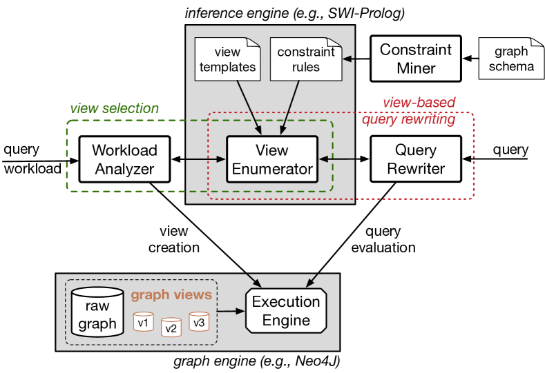
Kaskade’s architecture is depicted in Figure 2. Users submit queries in a language that includes graph pattern constructs expressed in Cypher [12, 13] and relational constructs expressed in SQL. They use the former to express path traversals, and the latter for filtering and aggregation operations. This query language, described in § III, is capable of capturing many of the applications described above.
Kaskade supports two main view-based operations: (i) view selection, i.e., given a set of queries, identify the most useful views to materialize for speeding up query evaluation, accounting for a space budget and various cost components; and (ii) view-based query rewriting, i.e., given a submitted query, determine how it can be rewritten given the currently materialized views in the system to improve the query’s execution time by leveraging the views. These operations are detailed in § V. The workload analyzer drives view selection, whereas the query rewriter is responsible for the view-based query rewriting.
An essential component in both of these operations is the view enumerator, which takes as input a query and a graph schema, and produces candidate views for that query. A subset of these candidates will be selected for materialization during view selection and for rewriting a query during view-based query rewriting. As we show in § IV, Kaskade follows a novel constraint-based view enumeration approach. In particular, Kaskade’s constraint miner extracts (explicit) constraints directly present in the schema and queries, and uses constraint mining rules to derive further (implicit) constraints. Kaskade employs an inference engine (we use Prolog in our implementation) to perform the actual view enumeration, using a set of view templates it expresses as inference rules. Further, it injects the mined constraints during enumeration, leading to a significant reduction in the space of candidate views. Moreover, this approach allows us to easily include new view templates, extending the capabilities of the system, and alleviates the need for writing complicated code to perform the enumeration.
Kaskade uses an execution engine component to create the views that are output by the workload analyzer, and to evaluate the rewritten query output by the query rewriter. In this work, we use Neo4j’s execution engine [14] for the storage of materialized views, and to execute graph pattern matching queries. However, our query rewriting techniques can be applied to other graph query execution engines, so long as their query language supports graph pattern matching clauses.
III Preliminaries
III-A Graph Data Model
We adopt property graphs as our data model [15], in which both vertices and edges are typed and may have properties in the form of key-value pairs. This schema captures constraints such as domain and range of edge types. In our provenance graph example of § I-A, an edge of type “read” only connects vertices of type “job” to vertices of type “file” (and thus never connects two vertices of type “file”). As we show later, such schema constraints play an essential role in view enumeration (§ IV). Most mainstream graph engines [14, 16, 17, 18, 19, 20, 21] provide support for this data model (including the use of schema constraints).
III-B Query Language
To address our query language requirements discussed in § II, Kaskade combines regular path queries with relational constructs in its query language. In particular, it leverages the graph pattern specification from Neo4j’s Cypher query language [12] and combines it with relational constructs for filters and aggregates. This hybrid query language resembles that of recent industry offerings for graph-structured data analytics, such as those from AgensGraph DB [21], SQL Server [19], and Oracle’s PGQL [22].
As an example, consider the job blast radius use case introduced in § I (Fig. 1). Fig. 3 illustrates a query that combines OLAP and anchored path constructs to rank jobs in its blast radius based on average CPU consumption.
listings/blast_radius.sql
Specifically, the query in Fig. 3 ranks jobs up to hops away in the downstream of a job (q_j1). In the example query, this is accomplished in Cypher syntax by using a variable length path construct of up to hops (-[r*0..8]->) between two file vertices (q_f1 and q_f2), where the two files are endpoints of the first and last edge on the complete path, respectively.
Although we use the Cypher syntax for our graph queries, our techniques can be coupled with any query language, as long as it can express graph pattern matching and schema constructs.
III-C Graph Views
We define a graph view over a graph as the graph query to be executed against . This definition is similar to the one first introduced by Zhuge and Garcia-Molina [23], but extended to allow the results of to also contain new vertices and edges in addition to those in . A materialized graph view is a physical data object containing the results of executing over .
Kaskade can support a wide range of graph views through the use of view templates, which are essentially inference rules, as we show in § IV. Among all possible views, we identify two classes, namely connectors and summarizers, which are sufficient to capture most of the use cases that we have discussed so far. Intuitively, connectors result from operations over paths (i.e., path contractions), whereas summarizers are obtained via summarization operations (filters or aggregates) that reduce the number of edges and/or vertices in the original graph.
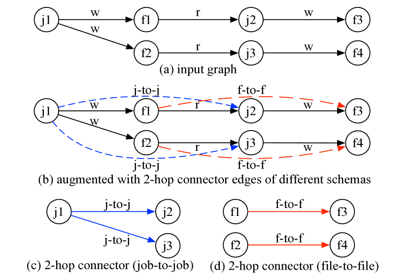
As an example, Fig. 4 shows the construction of -hop same-vertex-type connector views over a data lineage graph (similar to the graph of Fig. 1). In Fig. 4(a), the input graph contains two types of vertices, namely jobs (vertex labels with a prefix) and files (vertex labels with an prefix), as well as two types of edges, namely (a job writes to a file) and (a file is read by a job). Fig. 4(b) shows two different types of connector edges: the first contracts -hop paths between pairs of job vertices (depicted as blue dashed edges); the second contracts -hop paths between pairs of file vertices (depicted as red dashed edges). Finally, Fig. 4(c) shows the two resulting connector graph views: one containing only the job-to-job connector edges (left), and one with only the file-to-file connector edges (right).
We defer the formal definition and more examples of connectors and summarizers to § VI, given that we consider their definition as a means to an end rather than a fundamental contribution of this work. Here and in Sections IV and V, we only provide sufficient information over graph views for the reader to follow our techniques. As path operations tend to be the most expensive operations in graphs, our description will pivot mostly around connectors. Materializing such expensive operations can lead to significant performance improvements at query evaluation time. Moreover, the semantics of connectors is less straightforward than that of summarizers, which resemble their relational counterparts (filters and aggregates). Note, however, that the techniques described here are generic and apply to any graph views that can are expressible as view templates.
IV Constraint-Based View Enumeration
Having introduced a preliminary set of graph view types in § III-C (see also § VI for more examples), we now describe Kaskade’s view enumeration process, which generates candidate views for the graph expressions of a query. As discussed in § II, view enumeration is central to Kaskade (see Fig. 2), as it is used in both view selection and query rewriting, which are described in § V. Given that the space of view candidates can be considerable, and that view enumeration is on the critical path of view selection and query rewriting, its efficiency is crucial.
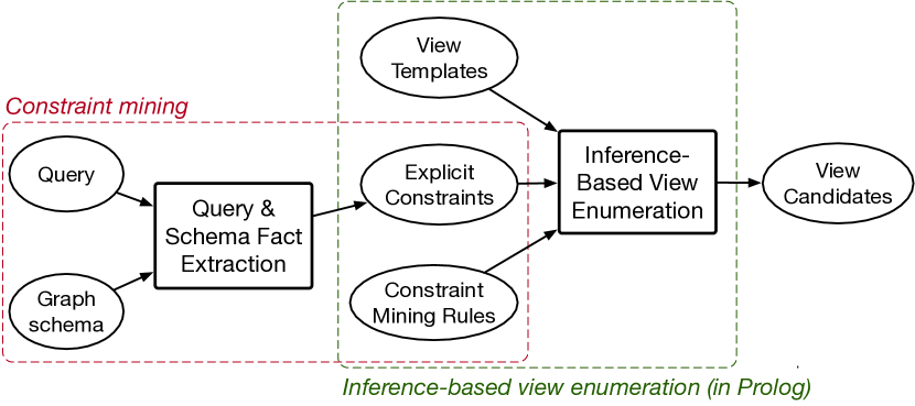
In Kaskade we use a novel approach, which we call constraint-based view enumeration. This approach mines constraints from the query and the graph schema and injects them at view enumeration time to drastically reduce the search space of graph view candidates. Fig. 5 depicts an overview of our approach. Our view enumeration takes as input a query, a graph schema and a set of declarative view templates, and searches for instantiations of the view templates that apply to the query. Kaskade expresses view templates as inference rules, and employs an inference engine (namely, Prolog)222While a subset of Kaskade’s constraint mining rules are expressible in Datalog, Prolog provides native support (i.e., without extensions) for aggregation and negation, and we use both in summarizer view templates. Kaskade also relies on higher-order predicates (e.g., setof, findall) in constraint mining rules, which Datalog does not support. to perform view enumeration through rule evaluation. Importantly, Kaskade generates both explicit constraints, extracted directly from the query and schema, and implicit ones, generated via constraint mining rules. This constraint mining process identifies structural properties from the schema and query that allow it to significantly prune the search space for view enumeration, discarding infeasible candidates (e.g., job-to-job edges or -hop connectors in our provenance example).
Apart from effectively pruning the search space of candidate views, Kaskade’s view enumeration provides the added benefit of not requiring the implementation of complex transformations and search algorithms—the search is performed by the inference engine automatically via our view templates and efficiently via the constraints that we mine. Moreover, view templates are readily extensible to modify the supported set of views. In our current implementation, we employ SWI-PL’s inference engine [24], which gives us the flexibility to seamlessly add new view templates and constraint mining rules via Prolog rules. On the contrary, existing techniques for view enumeration in the relational setting typically decompose a query through a set of application-specific transformation rules [25] or by using the query optimizer [26], and then implement search strategies to navigate through the candidate views. Compared to our constraint-based view enumeration, these approaches require higher implementation effort and are inflexible when it comes to adding or modifying complex transformation rules.
We detail the two main parts of our constraint-based view enumeration, namely the constraint mining and the inference-based view enumeration, in Sections IV-A and IV-B, respectively.
IV-A Mining Structural Graph Constraints
Kaskade exploits information from the graph’s schema and the given query in the form of constraints to prune the set of candidate views to be considered during view enumeration. It mines two types of constraints:
-
•
Explicit constraints (§ IV-A1) are first-order logic statements (facts) extracted from the schema and query (e.g., that files do not write files, only jobs);
-
•
Implicit constraints (§ IV-A2) are not present in the schema or query, but are derived by combining the explicit constraint facts with constraint mining rules. These constraints are essential in Kaskade, as they capture structural properties that otherwise cannot be inferred by simply looking at the input query or schema properties.
IV-A1 Extracting explicit constraints
The first step in our constraint-based view enumeration is to extract explicit constraints (facts) from the query and schema.
Transforming the query to facts. Our view enumeration algorithm goes over the query’s MATCH clause, i.e., its graph pattern matching clause, and for each vertex and edge in the graph pattern, Kaskade’s constraint miner emits a set of Prolog facts. In our running example of the job “blast radius” query (Fig. 3), Kaskade extracts the following facts from the query:
queryVertex(q_f1). queryVertex(q_f2). queryVertex(q_j1). queryVertex(q_j2). queryVertexType(q_f1, ’File’). queryVertexType(q_f2, ’File’). queryVertexType(q_j1, ’Job’). queryVertexType(q_j2, ’Job’). queryEdge(q_j1, q_f1). queryEdge(q_f2, q_j2). queryEdgeType(q_j1, q_f1, ’WRITES_TO’). queryEdgeType(q_f2, q_j2, ’IS_READ_BY’). queryVariableLengthPath(q_f1, q_f2, 0, 8).
The above set of facts contains all named vertices and edges in the query’s graph pattern, along with their types, and any variable-length regular path expression (queryVariableLengthPath( X,Y,L,U) corresponds to a path between nodes X and Y of length between L and U). In Fig. 3, a variable-length regular path of up to 8 hops is specified between query vertices q_f1 and q_f2.
Transforming the schema to facts. Similar to the extraction of query facts, our view enumeration algorithm goes over the provided graph schema and emits the corresponding Prolog rules. For our running example of the data lineage graph, there are two types of vertices (files and jobs) and two types of edges representing the producer-consumer data lineage relationship between them. Hence, the set of facts extracted about this schema is:
schemaVertex(’Job’). schemaVertex(’File’). schemaEdge(’Job’, ’File’, ’WRITES_TO’). schemaEdge(’File’, ’Job’, ’IS_READ_BY’).
IV-A2 Mining implicit constraints
Although the explicit query and schema constraints that we introduced so far restrict the view enumeration to consider only views with meaningful vertices and edges (i.e., that appear in the query and schema), they still allow many infeasible views to be considered. For example, if we were to enumerate -hop connectors between two files to match the variable-length path in the query of Fig. 3, all values of would have to be considered. However, given the example schema, we know that only even values of are feasible views. Similarly, since the query specifies an upper limit in the number hops in the variable-length path, we should not be enumerating -hop connectors with .
To derive such implicit schema and query constraints that will allow us to significantly prune the search space of views to consider, Kaskade uses a library of constraint mining rules333The collection of constraint mining rules Kaskade provides is readily extensible, and users can supply additional constraint mining rules if desired. for the schema and query. Fig. 6 shows an example of such a constraint mining rule for the schema. Rule schemaKHopPath, expressed in Prolog in the listing, infers all valid -hop paths given the input schema. Note that the rule takes advantage of the explicit schema constraint schemaEdge to derive this more complex constraint from the schema, and it considers two instances of schemaKHopPath different if and only if all values in the resulting unification tuple are different. For example, a schemaKHopPath(X=‘Job’,Y=‘Job’,K=2) unification, i.e., a job-to-job 2-hop connector is different from a schemaKHopPath(X=‘File’,Y=‘File’,K=2), i.e., a file-to-file 2-hop connector. For completeness, we also provide a procedural version of this constraint mining rule in Appendix B (Alg. 1). When contrasted with the Prolog rule, the procedural version is not only more complex, but it also explores a larger search space. This is because the procedural function cannot be injected at view enumeration time as an additional rule together with other inference rules that further bound the search space (see § IV-B).
listings/structural_properties.pl
Similar constraint mining rules can be defined for the query. Appendix B (Fig. 13) shows examples of such rules, e.g., to bound the length of considered -hop connectors (in case such limits are present in the query’s graph pattern), or to ensure that a node is the source or sink in a connector.
These constraints play a crucial role in limiting the search space for valid views. As we show in § IV-B, by injecting such rules at view enumeration time, Kaskade can automatically derive implicit knowledge from the schema and query to significantly reduce the search space of considered views. Interestingly, Kaskade can derive this knowledge only on demand, in that the constraint mining rules get fired only when required and do not blindly derive all possible facts from the query and schema.
Importantly, the combination of both schema and query constraints is what makes it possible for our view enumeration approach to reducing the search space of possible rewritings. As an example, consider the process of enumerating valid -hop connector views. Without any query constraints, the number of such views equals the number of -length paths over the schema graph, which has schema edges. While there exists no closed formula for this combination, when the schema graph has one or more cycles (e.g., a schema edge that connects a schema vertex to itself), at least -hop schema paths can be enumerated. This space is what the schemaKHopPath schema constraint mining rule would search over, were it not used in conjunction with query constraint mining rules on view template definitions. Kaskade’s constraint-based view inference algorithm enumerates a significantly smaller number of views for input queries, as the additional constraints enable its inference engine to efficiently search by early-stopping on branches that do not yield feasible rewritings.
IV-B Inference-based View Enumeration
listings/spanner_views.pl
As shown in Fig. 5, Kaskade’s view enumeration takes as input (i) a query, (ii) a graph schema, and (iii) a set of view templates. As described in § IV-A, the query and schema are used to mine explicit and implicit constraints. Both the view templates and the mined constraints are rules that are passed to an inference engine to generate candidate views via rule evaluation. Hence, we call this process inference-based view enumeration. The view templates drive the search for candidate views, whereas the constraints restrict the search space of considered views. This process outputs a collection of instantiated candidate view templates, which are later used either by the workload analyzer module (see Fig. 2) when determining which views to materialize during view selection (§ V-B), or by the query rewriter to rewrite the query using the materialized view (§ V-C) that will lead to its most efficient evaluation.
Fig. 7 shows examples of template definitions for connector views. Each view template is defined as a Prolog rule and corresponds to a type of connector view. For instance, kHopConnector(X,Y,XTYPE,YTYPE,K) corresponds to a connector of length K between nodes X and Y, with types XTYPE and YTYPE, respectively. An example instantiation of this template is kHopConnector(X,Y,‘Job’,‘Job’,2), which corresponds to a concrete job-to-job 2-hop connector view. This view can be translated to an equivalent Cypher query, which will be used either to materialize the view or to rewrite the query using this view, as we explain in § V. Other templates in the listing are used to produce connectors between nodes of the same type or source-to-sink connectors. Additional view templates can be defined in a similar fashion, such as the ones for summarizer views that we provide in Appendix A (Fig. 12).
Note that the body of the view template is defined using the query and schema constraints, either the explicit ones (e.g., queryVertexType) coming directly from the query or schema, or via the constraint mining rules (e.g., queryKHopPath, schemaKHopPath), as discussed in § IV-A. For example, kHopConnector’s body includes two explicit constraints to check the type of the two nodes participating in the connector, a query constraint mining rule that will check whether there is a valid -hop path between the two nodes in the query, and a schema constraint mining rule that will do the same check on the schema.
Having gathered all query and schema facts, Kaskade’s view enumeration algorithm performs the actual view candidate generation. In particular, it calls the inference engine for every view template. As an example, assuming an upper bound of — in Fig. 3 we have a variable-length path of at most 8 hops between 2 File vertices, and each of these two vertices is an endpoint for another edge — the following are valid instantiations of the kHopConnector(X,Y,XTYPE,YTYPE,K) view template for query vertices q_j1 and q_j2 (the only vertices projected out of the MATCH clause):
(X=’q_j1’, Y=’q_j2’, XTYPE=’Job’, XTYPE=’Job’, K=2) (X=’q_j1’, Y=’q_j2’, XTYPE=’Job’, XTYPE=’Job’, K=4) (X=’q_j1’, Y=’q_j2’, XTYPE=’Job’, XTYPE=’Job’, K=6) (X=’q_j1’, Y=’q_j2’, XTYPE=’Job’, XTYPE=’Job’, K=8) (X=’q_j1’, Y=’q_j2’, XTYPE=’Job’, XTYPE=’Job’, K=10)
Or, in other words, the unification (X=‘q_j1’, Y=‘q_j2’, XTYPE=‘Job’, XTYPE=‘Job’, K=2) for the view template kHopConnector(X,Y,XTYPE,YTYPE,K) implies that a view where each edge contracts a path of length between two nodes of type Job is feasible for the query in Fig. 3.
Similarly, Kaskade generates candidates for the remaining templates of Listings 7 and 12. For each candidate it generates, Kaskade’s inference engine also outputs a rewriting of the given query that uses this candidate view, which is crucial for the view-based query rewriting, as we show in § V-C. Finally, each candidate view incurs different costs (see § V-A), and not every view is necessarily materialized or chosen for a rewrite.
V View Operations
In this section, we present the main two operations that Kaskade supports: selecting views for materialization given a set of queries (§ V-B) and view-based rewriting of a query given a set of pre-materialized views (§ V-C). To do this, Kaskade uses a cost model to estimate the size and cost of views, which we describe next (§ V-A).
V-A View Size Estimation and Cost Model
While some techniques for relational cost-based query optimization may at times target filters and aggregates, most efforts in this area have primarily focused on join cardinality estimation [27]. This is in part because joins tend to dominate query costs, but also because estimating join cardinalities is a harder problem than, e.g., estimating the cardinality of filters. Furthermore, Kaskade can leverage existing techniques for cardinality estimation of filters and aggregates in relational query optimization for summarizers.
Therefore, here we detail our cost model contribution as it relates to connector views, which can be seen as the graph counterpart of relational joins. We first describe how we estimate the size of connector views, which we then use to define our cost model.
Graph data properties During initial data loading and subsequent data updates, Kaskade maintains the following graph properties: (i) vertex cardinality for each vertex type of the raw graph; and (ii) coarse-grained out-degree distribution summary statistics, i.e., the 50th, 90th, and 95th out-degree for each vertex type of the raw graph. Kaskade uses these properties to estimate the size of a view.
View size estimation. Estimating the size of a view is essential for the Kaskade’s view operations. First, it allows us to determine if a view will fit in a space budget during view selection. Moreover, our cost components (see below) use view size estimates to assess the benefit of a view both in view selection and view-based query rewriting.
In Kaskade, we estimate the size of a view as the number of edges that it has when materialized since the number of edges usually dominates the number of vertices in real-world graphs. Next, we observe that the number of edges in a -hop connector over a graph equals the number of -length simple paths in . We considered using the following estimator for Erdos-Renyi random graphs [28], where edges are generated uniformly at random, and the expected number of -length simple paths can be computed as:
| (1) |
where is the number of vertices in , and is the number of edges in . However, we found that for real-world graphs, the independence assumption does not hold for vertex connectivity, as the degree distributions are not necessarily uniform and edges are usually correlated. As a result, this formula significantly underestimates — by several orders of magnitude — the number of directed -length paths in real-world graphs. Therefore, for a directed graph that is homogeneous (i.e., has only one type of vertex, and one type of edge), we define the following estimator for its number of -length paths:
| (2) |
where is the number of vertices in , and is the -th percentile out-degree of vertices in (.
For a directed graph that is heterogeneous (i.e., has more than one type of vertex and/or more than one type of edge), an estimator for its number of -length paths is as follows:
| (3) |
where is the set of types of vertices in that are edge sources (i.e., are the domain of at least one type of edge), is the number of vertices of type , and is the maximum out-degree of vertices of type .
Observe that if , then is the maximum out-degree and the estimators above are upper bounds on the number of -length paths in the graph. This is because there are possible starting vertices, each vertex in the path has at most (or ) neighbors to choose from for its successor vertex in the path, and such a choice has to be made times in a -length path. In practice, we found that gives a very loose upper bound, whereas gives a much more accurate estimate depending on the degree distribution of the graph. We present experiments on the accuracy of our estimator in § VII.
View creation cost. The creation cost of a graph view refers to any computational and I/O costs incurred when computing and materializing the views’ results. Since the primitives required for computing and materializing the results of the graph views that we are interested in are relatively simple, the I/O cost dominates computational costs, and thus the latter is omitted from our cost model. Hence, the view creation cost is directly proportional to .
Query evaluation cost. The cost of evaluating a query , denoted , is required both in the view selection and the query rewriting process. Kaskade relies on an existing cost model for graph database queries as a proxy for the cost to compute a given query using the raw graph. In particular, it leverages Neo4j’s [14] cost-based optimizer, which establishes a reasonable ordering between all vertex scans without indexes, scans from indexes, and range scans. As part of our future work, we plan to incorporate our findings from graph view size estimation to further improve the query evaluation cost model.
V-B View Selection
Given a query workload, Kaskade’s view selection process determines the most effective views to materialize for answering the workload under the space budget that Kaskade allocates for materializing views. This operation is performed by the workload analyzer component, in conjunction with the view enumerator (see § IV). The goal of Kaskade’s view selection algorithm is to select the views that lead to the most significant performance gains relative to their cost, while respecting the space budget.
To this end, we formulate the view selection algorithm as a 0-1 knapsack problem, where the size of the knapsack is the space budget dedicated to view materialization.444The space budget is typically a percentage of the machine’s main memory size, given that we are using a main memory execution engine. Our formulation can be easily extended to support multiple levels of memory hierarchy. The items that we want to fit in the knapsack are the candidate views generated by the view enumerator (§ IV). The weight of each item is the view’s estimated size (see § V-A), while the value of each item is the performance improvement achieved by using that view divided by the view’s creation cost (to penalize views that are expensive to materialize). We define the performance improvement of a view for a query in the query workload as ’s evaluation cost divided by the cost of evaluating the rewritten version of that uses . The performance improvement of for is the sum of ’s improvement for each query in (which is zero for the queries for which is not applicable). Note that we can extend the above formulation by adding weights to the value of each query to reflect its relative importance (e.g., based on the query’s frequency to prioritize more frequent queries, or on the query’s estimated execution time to prioritize more expensive queries).
The views that the above process selects for materialization are instantiations of Prolog view templates output by the view enumeration (see § IV). Kaskade’s workload analyzer translates those views to Cypher and executes them against the graph to perform the actual materialization. As a byproduct of this process, each combination of query and materialized view is accompanied by a rewriting of using , which is crucial in the view-based query rewriting, described next. The rewriter component converts the rewriting in Prolog to Cypher, so that Kaskade can run it on its graph execution engine.
V-C View-Based Query Rewriting
Given a query and a set of materialized views, view-based rewriting is the process of finding the rewriting of the query that leads to the highest reduction of its evaluation cost by using (a subset of) the views. In Kaskade, the query rewriter module (see Fig. 2) performs this operation.
When a query arrives in the system, the query rewriter invokes the view enumerator, which generates the possible view candidates for , pruning those that it has not materialized. Among the views that are output by the enumerator, the query rewriter selects the one that, when used to rewrite , leads to the smallest evaluation cost for . As discussed in § IV, the view enumerator outputs the rewriting of each query based on the candidate views for that query. If this information is saved from the view selection step (which is true in our implementation), we can leverage it to choose the most efficient view-based rewriting of the query without having to invoke the view enumeration again for that query. As we mentioned in § IV, Kaskade currently supports rewritings that rely on a single view. Combining multiple views in a single rewriting is left as future work.
Fig. 8 shows the rewritten version of our example query of Fig. 3 that uses a 2-hop connector (“job-to-job”) graph view.
listings/blast_radius_2_hop.sql
VI View Definitions and Examples
Next we provide formal definitions of the two main classes of views supported in Kaskade, namely connectors and summarizers, which were briefly described in § III-C. Moreover, we give various examples of the views from each category that are currently present in Kaskade’s view template library.
While the examples below are general enough to capture many different types of graph structures, they are by no means an exhaustive list of graph view templates that are possible in Kaskade; as we mention in § IV, Kaskade’s library of view templates and constraint mining rules is readily extensible.
VI-A Connectors
| Type | Description |
|---|---|
| Same-vertex-type connector | Target vertices are all pairs of vertices with a specific vertex type. |
| -hop connector | Target vertices are all vertex pairs that are connected through -length paths. |
| Same-edge-type connector | Target vertices are all pairs of vertices that are connected with a path consisting of edges with a specific edge type |
| Source-to-sink connector | Target vertices are (source, sink) pairs, where sources are the vertices with no incoming edges and sinks are vertices with no outgoing edges. |
A connector of a graph is a graph such that every edge is obtained via contraction of a single directed path between two target vertices . The vertex set of the connector view is the union of all target vertices with . Based on this definition, a number of specialized connector views can be defined, each of which differs in the target vertices that it considers. Table I lists examples currently supported in Kaskade.
Additionally, it is easy to compose the definition of -hop connectors with the other connector definitions, leading to more connector types. As an example, the -hop same-vertex-type connector is a same-vertex-type connector with the additional requirement that the target vertices should be connected through -hop paths.
Finally, connectors are useful in contexts where a query’s graph pattern contains relatively long paths that can be contracted without loss of generality, or when only the endpoints of the graph pattern are projected in subsequent clauses in the query.
| Type | Description |
|---|---|
| Vertex-removal summarizer | Removes vertices and connected edges that satisfy a given predicate, e.g., vertex type or vertex property. |
| Edge-removal summarizer | Removes edges that satisfy a given predicate. |
| Vertex-inclusion summarizer | Includes vertices that satisfy the predicate, and edges where both the source and target vertices satisfy the predicate. |
| Edge-inclusion summarizer | Includes only edges that satisfy a given predicate. |
| Vertex-aggregator summarizer | Groups vertices that satisfy a given predicate, and combines them using the provided aggregate function. |
| Edge-aggregator summarizer | Groups edges that satisfy a given predicate, and combines them using the provided aggregate function. If the resulting edges do not have the same source and destination vertices, it also performs a vertex aggregation operation. |
| Subgraph-aggregator summarizer | Groups both edges and vertices that satisfy a given predicate, and combines them using the provided aggregate function. |
VI-B Summarizers
A summarizer of a graph is a graph such that , , and at least one of the following conditions are true: (i) , or (ii) . The summarizer view operations that Kaskade currently provides are filters that specify the type of vertices or edges that we want to preserve (inclusion filters) or remove (exclusion filters) from the original graph.555Summarizer views can also include predicates on vertex/edge properties in their definitions. Using such predicates would further reduce the size of these views, but given they are straightforward, here we focus more on predicates for vertex/edge types. Also, it provides aggregator summarizers that either group a set of vertices into a supervertex, a group of edges into a superedge, or a subgraph into a supervertex. Finally, aggregator summarizers require an aggregate function for each type of property present in the domain of the aggregator operation. Examples of summarizer graph views currently supported are given in Table II. Kaskade’s library of template views currently does not support aggregation of vertices of different types. The library is readily extensible, however, and aggregations for vertices or edges with different types are expressible using a higher-order aggregate function to resolve conflicts between properties with the same name, or to specify the resulting aggregate type.
Lastly, summarizers can be useful when subsets of data (e.g., entire classes of vertices and edges) can be removed from the graph without incurring any side-effects (in the case of filters), or when queries refer to logical entities that correspond to groupings of one or more entity at a finer granularity (in the case of aggregators).
VII Experimental Evaluation
In this section, we experimentally confirm that by leveraging graph views (e.g., summarizers and connectors) we can: (i) accurately estimate graph view sizes—§ VII-D; (ii) effectively reduce the graph size our queries operate on—§ VII-E; and (iii) improve query performance—§ VII-F. We start by providing details on Kaskade’s current implementation, and follow by introducing our datasets and query workload.
VII-A Implementation
We have implemented Kaskade’s components (see Fig. 2) as follows. The view enumerator component (§ IV) uses SWI-Prolog [24] as its inference engine. We wrote all constraint mining rules, query constraint mining rules, and view templates using SWI-Prolog syntax, which is close to ISO-Prolog [29]. We wrote the knapsack problem formulation (§ V-B) in Python 2.7, using the branch-and-bound knapsack solver from Google OR tools combinatory optimization library [30]. As shown in Fig. 2, Kaskade uses Neo4J (version 3.2.2) for storage of raw graphs, materialized graph views, and query execution of graph pattern matching queries. All other components — including the constraint miner — were written in Java.
For the experimental results below, Kaskade extracted schema constraints only once for each workload, as these do not change throughout the workload. Furthermore, Kaskade extracted query constraints as part of view inference only the first time we entered the query into the system. This process introduces a few milliseconds to the total query runtime — as the number of query facts combined with schema facts is small, and in the experiments below we focus on one type of view template — and is amortized for multiple runs of the same query.
VII-B Datasets
In our evaluation of different aspects of Kaskade, we use a combination of publicly-available heterogeneous and homogeneous networks and a large provenance graph from Microsoft (heterogeneous network). Table III lists the datasets and their raw sizes. We also provide their degree distributions in Appendix C.
| Short Name | Type | ||
|---|---|---|---|
| prov (raw) | Data lineage | 3.2B | 16.4B |
| prov (summarized) | Data lineage | 7M | 34M |
| dblp-net | Publications [31] | 5.1M | 24.7M |
| soc-livejournal | Social network [32] | 4.8M | 68.9M |
| roadnet-usa | Road network [7] | 23.9M | 28.8M |
For our size reduction evaluation in Section VII-E, we focus on gains provided by different graph views over the two heterogeneous networks: dblp-net and a data lineage graph from Microsoft. The dblp-net graph, which is publicly available at [31], contains 5.1M vertices (authors, articles, and venues) with 24.7M with 2.2G on-disk footprint. For the second heterogeneous network, we captured a provenance graph modeling one of Microsoft’s large production clusters for a week. This raw graph contains 3.2B vertices modeling jobs, files, machines, and tasks, and 16.4B edges representing relationships among these entities, such as job-read-file, or task-to-task data transfers. The on-disk footprint of this data is in the order of 10+ TBs.
After showing size reduction achieved by summarizers and connectors in Section VII-E, for our query runtime experiments (§ VII-F), we consider already summarized versions of our heterogeneous networks, i.e., of dblp-net and provenance graph. The summarized graph over dblp-net contains only authors and publications (“article”, “publication”, and “in-proc” vertex types), totaling 3.2M vertices and 19.3M edges, which requires 1.3G on disk. The summarized graph over the raw provenance graph contains only jobs and files and their relationships, which make up its 7M vertices and 34M edges. The on-disk footprint of this data is 4.8 GBs. This allows us to compare runtimes of our queries on the Neo4j 3.2.2 graph engine, running on a 128 GB of RAM and 28 Intel Xeon 2.40GHz cores, 4 x 1TB SSD Ubuntu box. We chose to use Neo4j for storage of materialized views and query execution because it is the most widely used graph database engine as of writing, but our techniques are graph query engine-agnostic.
VII-C Queries
Table IV lists the queries that we use in our evaluation of query runtimes. Queries Q1 through Q3 are motivated by telemetry use cases at Microsoft, and are defined as follows. The first query retrieves the job blast radius, up to 8 hops away, of all job vertices in the graph, together with their average CPU consumption property. Query Q2 retrieves the ancestors of a job (i.e., all vertices in its backward data lineage) up to 4 hops away, for all job vertices in the graph. Conversely, Q3 does the equivalent operation for forward data lineage for all vertices in the graph, also capped at 4 hops from the source vertex. Both Q2 and Q3 are also adapted for the other 3 graph datasets: on dblp, the source vertex type is “author” instead of “job”, and on homogeneous networks roadnet-usa and soc-livejournal all vertices are included.
| Query | Operation | Result |
|---|---|---|
| Q1: Job Blast Radius | Retrieval | Subgraph |
| Q2: Ancestors | Retrieval | Set of vertices |
| Q3: Descendants | Retrieval | Set of vertices |
| Q4: Path lengths | Retrieval | Bag of scalars |
| Q5: Edge Count | Retrieval | Single scalar |
| Q6: Vertex Count | Retrieval | Single scalar |
| Q7: Community Detection | Update | N/A |
| Q8: Largest Community | Retrieval | Subgraph |
Next, queries Q4 through Q7 capture graph operation primitives which are commonly required for tasks in dependency driven analytics [4]. The first, query Q4 (“path lengths”), computes a weighted distance from a source vertex to all other vertices in its forward -hop neighborhood, limited to 4 hops. It does so by first retrieving all vertices in a given vertex’s 4-hop neighborhood, and then for each vertex in this result set, it performs an aggregation operation (max) over a data property (edge timestamp) of all edges in the path. Queries Q5 and Q6 both measure the overall size of the graph (edge count and vertex count, respectively).
Finally, Q7 (“community detection”) and Q8 (“largest community”) are representative of common graph analytics tasks. The former runs a 25 passes iterative version of community detection algorithm via label-propagation, updating a community property on all vertices and edges in the graph, while Q8 uses the community label produced by Q7 to retrieve the largest community in terms of graph size as measured by number of “job” vertices in each community. The label propagation algorithm used by Q7 is part of the APOC collection of graph algorithm UDFs for Neo4j [33].
For query runtimes experiments in § VII-F, we use the equivalent rewriting of each of these queries over a -hop connector. Specifically, queries Q1 through Q4 go over half of the original number of hops, and queries Q7 and Q8 run around half as many iterations of label propagation. These rewritings are equivalent and produce the same results as queries Q1 through Q4 over the original graph, and similar groupings of “job” nodes in the resulting communities. Queries Q5 and Q6 need not be modified, as they only count the number of elements in the dataset (edges and vertices, respectively).
VII-D View Size Estimation
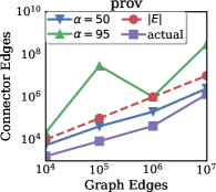
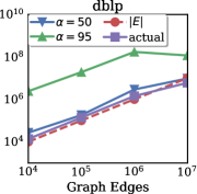
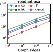
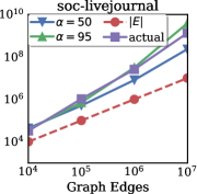
In this section, we evaluate the accuracy of Kaskade’s view size estimators (§ V-A). Fig. 9 shows our results for different heuristics estimators on the size of a -hop connector view materialized over the first edges of each public graph dataset. We focus on size estimates for -hop connectors since, similar to cardinality estimation for joins, the larger the , the less accurate our estimator. We do not report results for view size estimates for summarizers, as for these Kaskade can leverage traditional cardinality estimation based on predicate selectivity for filters, as well as multi-dimensional histograms for predicate selectivity of group-by operators [27].
We found that -hop connectors in homogeneous networks are usually larger than the original graph in real-world networks. This is because -length paths can exist between any two vertices in this type of a graph, as opposed to only between specific types of vertices in heterogeneous networks, such as Microsoft’s provenance graph. Note that the line does a good job of approximating the size of the graph as the number of edges grows. Also, for networks with a degree distribution close to a power-law, such as soc-livejournal, the estimator that relies on 95th percentile out-degree () provides an upper bound, while the one that uses the median out-degree () of the network provides a lower bound. On other networks that do not have a power-law degree distribution, such as road-net-usa, the median out-degree estimator better approximates an upper bound on the size of the -hop connector.
In practice, Kaskade relies on the estimator parameterized with as it provides an upper bound for most real-world graphs that we have observed. Also note that the estimator with for prov decreases when the original graph increases in size from to edges, increasing again at edges. This is due to a decrease in the percentage of “job” vertices with a large out-degree, shifting the 95th percentile to a lower value. This percentile remains the same at edges, while the 95th out-degree for “file” vertices increases at both and edges.
VII-E Size Reduction
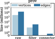
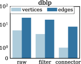
This experiment shows how by applying summarizers and connectors over heterogeneous graphs we can reduce the effective graph size for one or more queries. Figure 10 shows that for co-authorship queries over the dblp, and query Q1 over the provenance graph, the schema-level summarizer yields up to three orders of magnitude reduction. The connector yields another two orders of magnitude data reduction by summarizing the job-file-job paths in the provenance graph, and one order of magnitude by summarizing the author-publication-author paths in the dblp graph.
Besides the expected performance advantage since queries operate on less data, such a drastic data reduction allows us to benefit from single-machine in-memory technologies (such as Neo4j) instead of slower distributed on-disk alternatives for query evaluation, in the case of the provenance graph. While this is practically very relevant, we do not claim this as part of our performance advantage, and all experiments are shown as relative speed-ups against a baseline on this provenance reduced graph, with all experiments on the same underlying graph engine.
VII-F Query Runtimes
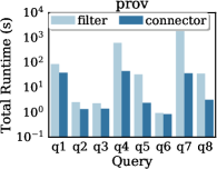
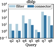
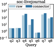
This experiment measures the difference in total query runtime for queries when executed from scratch over the filtered graph versus over an equivalent connector view on the filtered graph. Figure 11 shows our results, with runtimes averaged over 10 runs, plotted in log scale on the -axis. Because the amount of data required to answer the rewritten query is up to orders of magnitude smaller (§ VII-E) in the heterogeneous networks, virtually every query over the prov and dblp graphs benefit from executing over the connector view. Specifically, Q2 and Q3 have the least performance gains (less than 2 times faster), while Q4 and Q8 obtain the largest runtime speedups (13 and 50 times faster, respectively). This is expected: Q2 (“ancestors”) and Q3 (“descendants”) explore a -hop ego-centric neighborhood in both the filtered graph and in the connector view that is of the same order of magnitude. Q4 (“path lengths”) and Q8 (“community detection”), on the other hand, are queries that directly benefit from the significant size reduction of the input graph. In particular, the maximum number of paths in a graph can be exponential on the number of vertices and edges, which affects both the count of path lengths that Q4 performs, as well as the label-propagation updates that Q8 requires. Finally, we also observe that because Kaskade creates connector views through graph transformations that are engine-agnostic, these gains should be available in other systems as well.
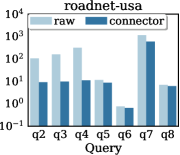
For the homogeneous networks, we look at the total query runtimes over the raw graph and over a vertex-to-vertex materialized -hop connector, which may be up to orders of magnitude larger than the raw graph (§ VII-D), as these networks have only one type of edge. Despite these differences in total sizes, a non-intuitive result is that the total query runtime is still linearly correlated with the order of magnitude increase in size for the network with a power-law degree distribution (soc-livejournal), while it decreases for path-related queries in the case of roadnet-usa. This is due to a combination of factors, including the larger fraction of long paths in roadnet-usa. Lastly, while the decision on which views to materialize heavily depends on the estimated view size (e.g., size budget constraints, and proxy for view creation cost), we note that these -hop connector views are unlikely to be materialized for the two homogeneous networks, due to the large view sizes predicted by our cost model, as shown in Figure 9.
VIII Related Work
Views and language. Materialized views have been widely used in the relational setting to improve query runtime by amortizing and hiding computation costs [34]. This inspires our work, but the topological nature of graph views makes them new and different. The notion of graph views and algorithms for their maintenance was first introduced in[23] by Zhuge and Garcia-Molina in 1998, but since then there has been little attention in this area. With Kaskade, we aim at providing a practical approach that can be used to deal with large-scale graphs. In particular, Kaskade addresses various problems related to graph views, including view enumeration, selection, as well as view-based query rewriting. In this paper, we focus on extracting views for the graph traversal portion of our queries, since these are the most crucial for performance. An interesting avenue for future work is to address a combined analysis of the relational and graph query fragments, related to what [35] proposes for a more restricted set of query types or [36] does for OLAP on graphs scenarios. The challenge is to identify and overcome the limits of relational query containment and view rewriting techniques for our hybrid query language.
Fan et al. [37] provide algorithms to generate views for speeding up fixed-sized subgraph queries, whereas Kaskade targets traversal-type queries that can contain an arbitrary number of vertices/edges. They do not provide a system for selecting the best views to generate based on a budget constraint. Le et al. [38] present algorithms for rewriting queries on SPARQL views, but do not have a system for selecting views. Katsifodimos et al. [39] present techniques for view selection to the improve performance of XML queries, which are limited to trees due to the structure of XML.
Graph engines. Kaskade is a graph query optimization framework that proposes a novel constraint-based view inference technique for materialized view selection and query rewriting. Although it is not a graph engine itself, in its current design it ultimately acts as one. We believe, however, that existing graph query execution engines may be able to leverage Kaskade for query optimization. Therefore, we group existing graph data management approaches based on their main focus: specialized databases for graph queries, including single-machine solutions, such as Neo4j [14] and TinkerPop [40], and distributed approaches, such as Datastax Graph Engine [41], TitanDB [17], CosmosDB [42]; large scale graph analytics, including Pregel [43], GraphLab [44], GraphX [16], Ligra [45], and EmptyHeaded [46] (see [8, 9] for surveys of graph processing systems); relational engines with graph support, such as SQLServer 2017 [19], Oracle [20], Spark GraphFrames [47], Agensgraph [21]; and graph algorithm libraries, such as NetworkX [48]. Our approach is mostly independent of the underlying graph engine, and while we run our experiments on Neo4J, Kaskade is directly applicable to any engine supporting Cypher [12] (or SQL+Cypher).
RDF and XML. The Semantic Web literature has explored the storage and inference retrieval of RDF and OWL data extensively [49]. While most efforts focused on indexing and storage of RDF triples, there has also been work on maintenance algorithms for aggregate queries over RDF data [50]. While relevant, this approach ignores the view selection and rewriting problems we consider here, and it has limited applicability outside RDF. RDFViewS [51] addresses the problem of view selection in RDF databases. However, the considered query and view language support pattern matching (which are translatable to relational queries) and not arbitrary path traversals, which are crucial in the graph applications we consider. Similar caveats are present in prior work on XML rewriting [52, 53], including lack of a cost model for view selection.
Graph summarization and compression. Graph summarization is the task of finding a smaller graph that is representative of the original graph to speed up graph algorithms or queries, for graph visualization, or to remove noise [54]. Most related to our work is the literature on using summarization to speed up graph computations for certain queries, where the answers can either be lossless or lossy [55, 56, 57, 58, 59]. As far as we know, prior work in this area has not explored the use of connectors and summarizers as part of a general system to speed up graph queries.
Rudolf et al. [60] describe several summarization templates in SAP HANA, which can be used to produce what we call graph views. However, their paper does not have a system that determines which views to materialize, and does not use the views to speed up graph queries.
IX Conclusions
We presented Kaskade, a graph query optimization framework that employs materialization to efficiently evaluate queries over graphs. Motivated by the fact that many application repeatedly run similar queries over the same graph, and that many production graphs have structural properties that restrict the types of vertices and edges that appear in graphs, Kaskade automatically derives graph views, using a new constraint-based view enumeration technique and a novel cost model that accurately estimates the size of graph views. We show in our experiments that queries rewritten over some of these views can provide up to 50 times faster query response times. Finally, the query rewriting techniques we have proposed are engine-agnostic (i.e., they only rely on fundamental graph transformations that typically yield smaller graphs, such as path contractions) and thus are applicable to other graph processing systems.
References
- [1] A. Ching et al., “One trillion edges: Graph processing at facebook-scale,” in PVLDB, 2015, pp. 1804–1815.
- [2] “Twitter.” https://twitter.com
- [3] A. Halevy et al., “Goods: Organizing google’s datasets,” in SIGMOD, 2016.
- [4] R. Mavlyutov et al., “Dependency-driven analytics: A compass for uncharted data oceans,” in CIDR 2017.
- [5] “DBpedia.” https://wiki.dbpedia.org
- [6] F. M. Suchanek, G. Kasneci, and G. Weikum, “Yago: a core of semantic knowledge,” in WWW, 2007, pp. 697–706.
- [7] “Network repository.” http://networkrepository.com
- [8] D. Yan et al., “Big graph analytics platforms,” Foundations and Trends in Databases, vol. 7, pp. 1–195, 2017.
- [9] R. R. McCune, T. Weninger, and G. Madey, “Thinking like a vertex: A survey of vertex-centric frameworks for large-scale distributed graph processing,” ACM Comput. Surv., vol. 48, pp. 25:1–25:39, Oct. 2015.
- [10] C. Curino et al., “Hydra: a federated resource manager for data-center scale analytics,” in NSDI, 2019.
- [11] “The EU general data protection regulation (GDPR).” https://www.eugdpr.org
- [12] “Cypher graph query language.” https://www.opencypher.org/
- [13] N. Francis et al., “Cypher: An evolving query language for property graphs,” in SIGMOD 2018, pp. 1433–1445.
- [14] “Neo4j graph database.” http://neo4j.org
- [15] “Property graphs.” https://www.w3.org/2013/socialweb/papers/Property_Graphs.pdf
- [16] J. E. Gonzalez et al., “Graphx: Graph processing in a distributed dataflow framework,” in OSDI, 2014, pp. 599–613.
- [17] “Titan distributed graph database.” http://thinkaurelius.github.io/titan
- [18] “Gremlin.” http://github.com/tinkerpop/gremlin/wiki
- [19] “Graph processing with SQL Server.” https://docs.microsoft.com/en-us/sql/relational-databases/graphs/sql-graph-overview
- [20] “Oracle parallel graph analytics (PGX).” http://www.oracle.com/technetwork/oracle-labs/parallel-graph-analytics
- [21] “AgensGraph Hybrid Graph Database.” http://www.bitnine.net
- [22] O. van Rest et al., “Pgql: A property graph query language,” in GRADES, 2016, pp. 7:1–7:6.
- [23] Y. Zhuge and H. Garcia-Molina, “Graph structured views and their incremental maintenance,” in ICDE, 1998, pp. 116–125.
- [24] “SWI-Prolog engine.” http://www.swi-prolog.org
- [25] T. K. Sellis, “Multiple-query optimization,” ACM Trans. Database Syst., vol. 13, pp. 23–52, 1988.
- [26] P. Roy et al., “Efficient and extensible algorithms for multi query optimization,” in SIGMOD 2000, pp. 249–260.
- [27] A. Deshpande, Z. Ives, and V. Raman, “Adaptive query processing,” Foundations and Trends in Databases, pp. 1–140, 2007.
- [28] B. Bollobas, Random Graphs. Cambridge University Press, 2001.
- [29] “SWI-Prolog syntax.” http://www.swi-prolog.org/man/syntax.html
- [30] “Google or tools - knapsacks.” https://developers.google.com/optimization/bin/knapsack
- [31] “Graphdblp.” https://github.com/fabiomercorio/GraphDBLP
- [32] “Snap livejournal dataset.” http://snap.stanford.edu/data/soc-LiveJournal1.html
- [33] “APOC graph algorithm udfs for neo4j.” https://neo4j-contrib.github.io/neo4j-apoc-procedures/#algorithms
- [34] A. Gupta and I. S. Mumick, in Materialized Views, 1999, ch. Maintenance of Materialized Views: Problems, Techniques, and Applications, pp. 145–157.
- [35] C. Lin et al., “Fast in-memory SQL analytics on typed graphs,” in VLDB 2016, pp. 265–276.
- [36] C. Chen et al., “Graph olap: Towards online analytical processing on graphs,” in ICDM, 2008, pp. 103–112.
- [37] W. Fan, X. Wang, and Y. Wu, “Answering pattern queries using views,” IEEE Transactions on Knowledge and Data Engineering, vol. 28, pp. 326–341, Feb 2016.
- [38] W. Le et al., “Rewriting queries on SPARQL views,” in International Conference on World Wide Web (WWW), 2011, pp. 655–664.
- [39] A. Katsifodimos, I. Manolescu, and V. Vassalos, “Materialized view selection for xquery workloads,” in ACM SIGMOD International Conference on Management of Data, 2012, pp. 565–576.
- [40] “Apache TinkerPop.” https://tinkerpop.apache.org/
- [41] “DataStax DSE graph engine.” https://www.datastax.com
- [42] R. Reagan, “Cosmos DB (chapter),” in Web Applications on Azure. Springer, 2018, pp. 187–255.
- [43] G. Malewicz et al., “Pregel: A system for large-scale graph processing,” in SIGMOD 2010, pp. 135–146.
- [44] Y. Low et al., “GraphLab: A new framework for parallel machine learning,” in UAI 2010, pp. 340–349.
- [45] J. Shun and G. E. Blelloch, “Ligra: A lightweight graph processing framework for shared memory,” in PPoPP 2013, pp. 135–146.
- [46] C. R. Aberger et al., “Emptyheaded: A relational engine for graph processing,” ACM Trans. Database Syst., vol. 42, pp. 20:1–20:44, Oct. 2017.
- [47] A. Dave et al., “GraphFrames: an integrated api for mixing graph and relational queries,” in GRADES, 2016.
- [48] “NetworkX python package for network data analysis.” https://networkx.github.io/
- [49] G. Antoniou and F. Van Harmelen, A semantic web primer. MIT press, 2004.
- [50] E. Hung, Y. Deng, and V. S. Subrahmanian, “Rdf aggregate queries and views,” in ICDE 2005, 2005.
- [51] F. Goasdoué et al., “View selection in semantic web databases,” in PVLDB, 2011, pp. 97–108.
- [52] N. Onose et al., “Rewriting nested xml queries using nested views,” in SIGMOD 2006, pp. 443–454.
- [53] W. Fan et al., “Rewriting regular xpath queries on xml views,” in ICDE 2007, pp. 666–675.
- [54] Y. Liu et al., “Graph summarization methods and applications: A survey,” ACM Comput. Surv., vol. 51, pp. 62:1–62:34, Jun. 2018.
- [55] W. Fan et al., “Query preserving graph compression,” in SIGMOD 2012, pp. 157–168.
- [56] S. Navlakha, R. Rastogi, and N. Shrivastava, “Graph summarization with bounded error,” in SIGMOD 2008, pp. 419–432.
- [57] K. Xirogiannopoulos and A. Deshpande, “Extracting and analyzing hidden graphs from relational databases,” in SIGMOD 2017, pp. 897–912.
- [58] N. Tang, Q. Chen, and P. Mitra, “Graph stream summarization: From big bang to big crunch,” in SIGMOD 2016, pp. 1481–1496.
- [59] C. Chen et al., “Mining graph patterns efficiently via randomized summaries,” in VLDB 2009, pp. 742–753.
- [60] M. Rudolf et al., “Synopsys: Large graph analytics in the sap hana database through summarization,” in GRADES 2013, pp. 16:1–16:6.
- [61] P. Boldi and S. Vigna, “The webgraph framework I: compression techniques,” in WWW 2004, pp. 595–602.
- [62] J. Shun, L. Dhulipala, and G. E. Blelloch, “Smaller and faster: Parallel processing of compressed graphs with Ligra+,” in DCC 2015, pp. 403–412.
- [63] A. Maccioni and D. J. Abadi, “Scalable pattern matching over compressed graphs via dedensification,” in KDD 2016, pp. 1755–1764.
Appendix A Example Summarizer View Templates
In § IV, we presented view templates in Prolog for connector views. Similarly, in Fig. 12, we provide example view templates for summarizer views.
listings/extraction_rules_b.pl
Appendix B Constraint Mining Rules
As discussed in § IV, Kaskade uses a set of constraint mining rules to extract implicit constraints from both schema and query graphs. In Fig. 13, we provide the Prolog definitions for some query constraint mining rules (for an example schema constraint mining rule, see § IV) used in Kaskade, such as path constraints over query graphs. In addition, Alg. 1 provides a procedural version of the schemaKHopPath example schema constraint mining rule of Fig. 6.
listings/extraction_rules_a.pl
Appendix C Degree Distributions
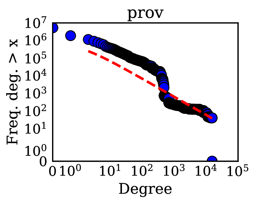
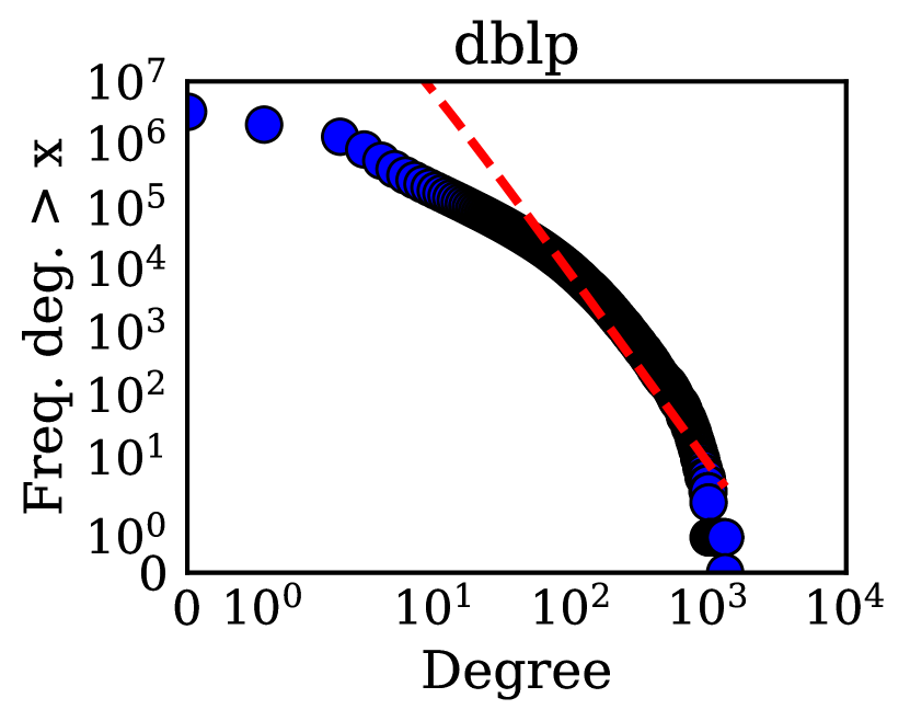
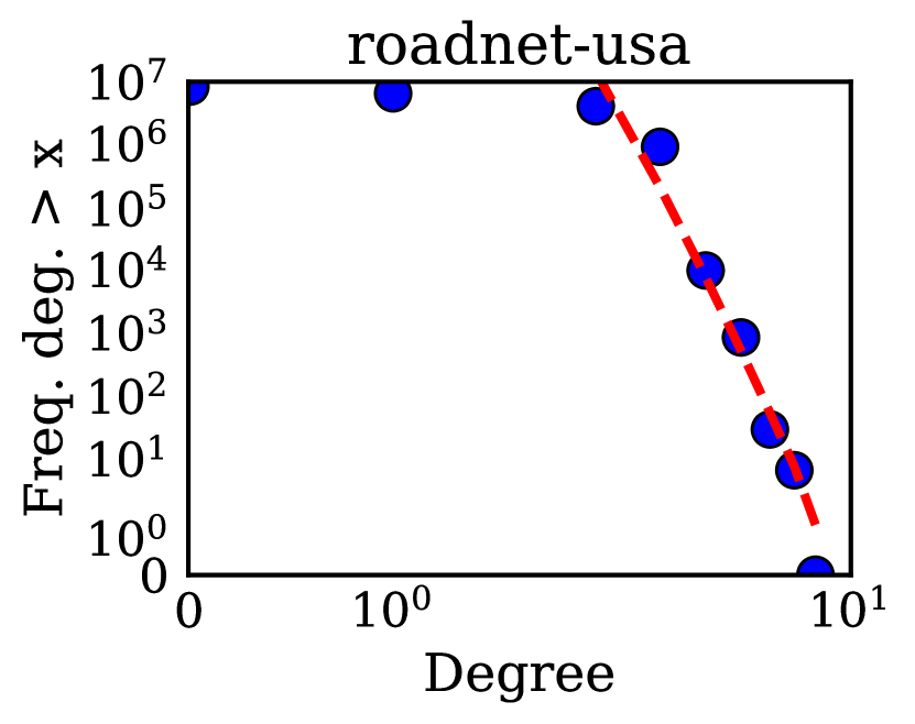
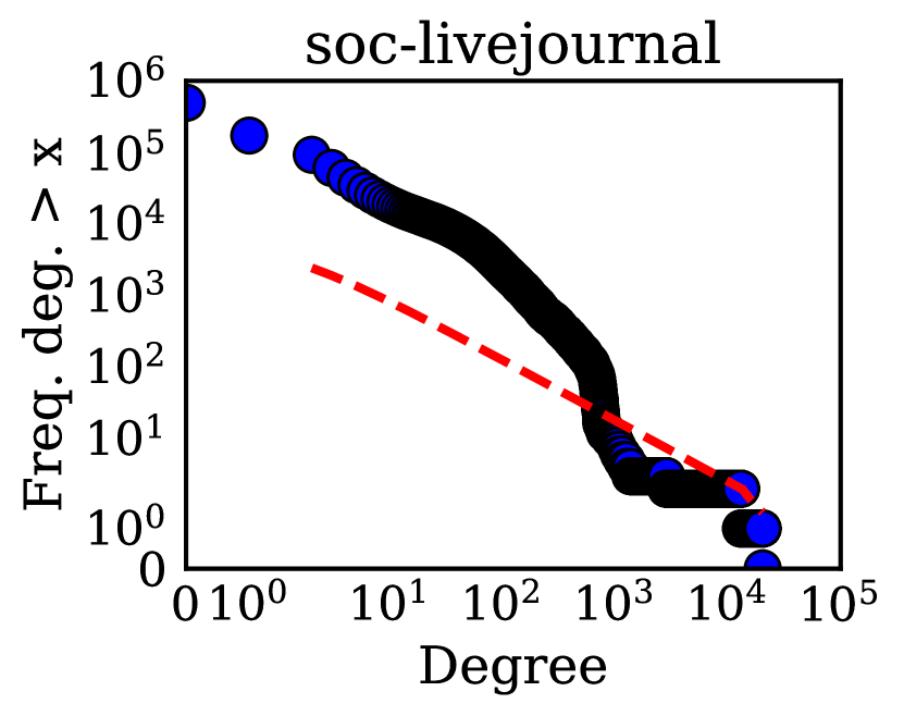
Fig. 14 shows the degree distributions of the different graphs used in our evaluation. As expected, vertex degrees in all but the road network dataset are roughly modeled by a power-law distribution, as evidenced by a goodness-of-linear-fit on log-log plot of the complementary cumulative distribution function (CCDF).
