Exploiting the Sign of the Advantage Function to
Learn Deterministic Policies in Continuous Domains

Abstract

In the context of learning deterministic policies in continuous domains, we revisit an approach, which was first proposed in Continuous Actor Critic Learning Automaton (CACLA) and later extended in Neural Fitted Actor Critic (NFAC). This approach is based on a policy update different from that of deterministic policy gradient (DPG). Previous work has observed its excellent performance empirically, but a theoretical justification is lacking. To fill this gap, we provide a theoretical explanation to motivate this unorthodox policy update by relating it to another update and making explicit the objective function of the latter. We furthermore discuss in depth the properties of these updates to get a deeper understanding of the overall approach. In addition, we extend it and propose a new trust region algorithm, Penalized NFAC (PeNFAC). Finally, we experimentally demonstrate in several classic control problems that it surpasses the state-of-the-art algorithms to learn deterministic policies.

1 Introduction

Model-free reinforcement learning combined with neural networks achieved several recent successes over a large range of domains Mnih et al. (2015); Lillicrap et al. (2016); Schulman et al. (2017). Yet those methods are still difficult to apply without any expert knowledge, lack robustness and are very sensitive to hyperparameter optimization Henderson et al. (2018); Colas et al. (2018).

In this context, we focus in this paper on improving methods that learn deterministic policies. Such policies have three main advantages during the learning phase: 1) they usually require less interactive data because fewer parameters need to be learned, 2) their performances are less costly to estimate during testing phases because randomness only comes from the environment (as opposed to randomized policies), and 3) they are also less sensitive to the premature convergence problem, because they cannot directly control exploration. Moreover, deterministic policies are preferred in some domains (e.g., robotics), because we do not want the agent to act stochastically after the learning phase.

In continuous state and action space domains, solution methods require function approximation. Neural control architectures are excellent representations for policies because they can handle continuous domains, are easily scalable, and have a high degree of expressiveness. The weights of such neural networks are usually updated with a policy gradient method. As vanilla policy gradient suffers from high variance, it is generally implemented in an actor-critic architecture where an estimated value function helps to reduce the variance at the cost of introducing some bias Konda and Tsitsiklis (1999). In this architecture, the parameters (e.g., weights of neural networks) of the policy (i.e., actor) and its value function (i.e., critic) are updated simultaneously.

The basic version of an actor-critic architecture for learning deterministic policies in continuous domains is the deterministic policy gradient (DPG) method Silver et al. (2014). Learning the value function is crucial but also difficult, which is why several extensions of DPG have been proposed. Deep Deterministic Policy Gradient (DDPG) Lillicrap et al. (2016) brings batch normalization Ioffe and Szegedy (2015), target networks and replay buffer Mnih et al. (2015) to DPG and is one of the most used actor-critic methods for learning continuous deterministic policies. However, it has several limitations: 1) the critic learns the state-action value function (Q function), which is difficult to estimate, 2) it relies on the fact that non-biased estimates of the gradient of the Q function are accessible, which is not the case in the model-free setting, 3) it does not use compatible functions: the policy gradient might be poorly estimated.

In this work, we focus on an alternative method that estimates the state value function (V function) instead of the Q function to learn continuous deterministic policies. Van Hasselt and Wiering Van Hasselt and Wiering (2007) were the first to propose to reinforce the policy toward an action with a positive temporal difference. They experimentally showed that using such a method, in an incremental actor-critic algorithm, called Continuous Actor Critic Learning Automaton (CACLA), provided better results than both the stochastic and the deterministic policy gradients in the Mountain Car and the Acrobot environments. Zimmer et al. Zimmer et al. (2016, 2018) validated those results in higher-dimensional environments, Half-Cheetah and Humanoid in Open Dynamic Engine Smith (2005), and proposed several extensions with the Neural Fitted Actor Critic (NFAC) algorithm. However, no theoretical explanation for their good performance, nor a clear discussion about which objective function those methods optimize were given. Providing such an explanation would help understand better why those algorithms work well, what are their properties and limitations, and how to further improve them.

We first show that CACLA and NFAC can be viewed as policy gradient methods and that they are closely related to a specific form of the stochastic policy gradient (SPG) Sutton et al. (1999). Then we discuss some of their properties and limitations. Moreover, we extend them with trust region updates and call the new algorithm Penalized Neural Fitted Actor Critic (PeNFAC). Finally, we experimentally show that PeNFAC performs well on three high-dimensional continuous environments compared to the state-of-the-art methods.

2 Background

A continuous Markov Decision Process (MDP) Sutton (1988) is a tuple $(\mathcal{S},\mathcal{A},T,R,T_{0})$ where $\mathcal{S}$ is a continuous state space, $\mathcal{A}$ is a continuous action space with $m$ dimensions, $T:\mathcal{S}\times\mathcal{A}\times\mathcal{S}\to[0,1]$ is a transition function, $R:\mathcal{S}\times\mathcal{A}\rightarrow\mathbb{R}$ is a reward function, $T_{0}$ is a distribution over initial states. In the model-free setting, it is assumed that the transition function $T$ and the reward function $R$ are unknown and can only be sampled at specific states according to the interaction between the agent and the environment.

The following notations are used: $\mu$ represents a deterministic policy and $\pi$ a stochastic one. Thus, for a given state $s\in\mathcal{S}$, $\mu(s)$ is an action, $\pi(a|s)$ is the probability of sampling action $a$ from the policy $\pi$, and $\pi(\cdot|s)$ is a distribution over the action space $\mathcal{A}$. For a policy $\pi$, we denote the discounted state distribution by:

$$d^{\pi}_{\gamma}(s)=\int_{\mathcal{S}}T_{0}(s_{0})\sum^{\infty}_{t=0}\gamma^{t}p(s|s_{0},t,\pi)ds_{0}$$

where $\gamma\in[0,1)$ is a discount factor and $p(s|s_{0},t,\pi)$ is the probability of being in state $s$ after applying policy $\pi$ $t$ timesteps from state $s_{0}$. Its state value function is defined by $V^{\pi}(s)$ $=$ $\mathbb{E}_{\pi}\big{[}\sum_{t=0}^{\infty}\gamma^{t}R(S_{t},A_{t})\big{|}S_{0}=s\big{]}$ where $\mathbb{E}_{\pi}$ is the expectation induced by $T$ and $\pi$, and for all $t$, $S_{t}$ and $A_{t}$ are random variables. Its action value function is given by $Q^{\pi}(s,a)=\mathbb{E}_{\pi}\big{[}\sum_{t=0}^{\infty}\gamma^{t}R(S_{t},A_{t})\big{|}S_{0}=s,A_{0}=a\big{]},$ and its advantage function by $A^{\pi}(s,a)=Q^{\pi}(s,a)-V^{\pi}(s)$.

In reinforcement learning, the goal is to find a policy that optimizes the expectation of the discounted rewards:

$$J(\pi)=\mathbb{E}_{\pi}\Big{[}\sum_{t=0}^{\infty}\gamma^{t}R(S_{t},A_{t})\big{|}S_{0}\sim T_{0}\Big{]}.$$

Due to the continuity of the state/action spaces, this optimization problem is usually restricted to a class of parametrized policies, which we denote $\pi_{\theta}$ (stochastic case) or $\mu_{\theta}$ (deterministic case). To simplify notations, we may write $\pi$ or $\mu$ instead of $\pi_{\theta}$ or $\mu_{\theta}$. The stochastic policy gradient (SPG) in the continuous case can be written as Sutton et al. (1999):

$$\nabla_{\theta}J(\pi)=\int_{\mathcal{S}}d^{\pi}_{\gamma}(s)\int_{\mathcal{A}}A^{\pi}(s,a)\nabla_{\theta}\pi_{\theta}(a|s)dads.$$ (1)

The DPG is defined as Silver et al. (2014):

$$\nabla_{\theta}J(\mu) =\int_{\mathcal{S}}d^{\mu}_{\gamma}(s)\Delta_{\text{DPG}}(s,\mu_{\theta})ds,$$ (2)

where

$$\Delta_{\text{DPG}}(s,\mu_{\theta}) =\nabla_{a}A^{\mu}(s,a)\big{|}_{a=\mu_{\theta}(s)}\nabla_{\theta}\mu_{\theta}(s).$$ (3)

Policy gradient methods usually take a step according to those directions: $\theta_{t+1}\leftarrow\theta_{t}+\alpha\nabla_{\theta}J$. However, it is difficult to select a proper learning rate $\alpha$ to control the step size. If $\alpha$ is too big, the method may diverge. If it is too low, the learning will converge slowly (thus requiring more samples). To overcome this difficulty, a trust region method can be used to control the step size Schulman et al. (2015). Indeed, one can guarantee monotonic gradient updates by exploiting an approximation of the policy advantage function Kakade and Langford (2002) of $\tilde{\pi}$ with respect to $\pi$, which measures the difference of performance between the two policies:

$$J(\tilde{\pi})= J(\pi)+\int_{\mathcal{S}}d^{\tilde{\pi}}_{\gamma}(s)\int_{\mathcal{A}}\tilde{\pi}(a|s)A^{\pi}(s,a)dads,$$ (4)

$$\approx J(\pi)+\int_{\mathcal{S}}d^{\pi}_{\gamma}(s)\int_{\mathcal{A}}\tilde{\pi}(a|s)A^{\pi}(s,a)dads.$$

The latter approximation holds when the two policies are close, which can be enforced by a KL divergence constraint in trust region policy optimization Schulman et al. (2015).

3 Algorithms

In this section, we recall three related algorithms (CACLA, CAC, NFAC) that we discuss later.

3.1 Continuous Actor Critic Learning Automaton

Continuous Actor Critic Learning Automaton (CACLA) Van Hasselt and Wiering (2007) is an actor-critic method that learns a stochastic policy $\pi$ and its estimated value function $\hat{V}^{\pi}$. We assume in this paper that CACLA uses isotropic Gaussian exploration, which implies that $\pi$ can be written as follows:

$$\pi_{\theta,\sigma}(\cdot|s)=\mathcal{N}\big{(}\mu_{\theta}(s),\sigma^{2}I)$$ (5)

where $I$ is the identity matrix and $\sigma>0$ possibly annealed during learning. CACLA alternates between two phases:

1) a hill climbing step in the action space using a random optimization (RO) algorithm Matyas (1965),

2) a gradient-like update in the policy parameter space. RO consists in repeating the following two steps:

i) sample a new action $a^{\prime}$, which is executed in the environment in current state $s$, by adding a normally distributed noise to the current action $a=\mu(s)$,

ii) if $R(s,a^{\prime})+\gamma\hat{V}^{\pi}(s^{\prime})>\hat{V}^{\pi}(s)$ then $a\leftarrow a^{\prime}$ else $a$ does not change.

Phase 2) is based on following update:

$$\text{If }\delta(s,a)>0:\tilde{\theta}\leftarrow\theta-\alpha\big{(}\mu_{\theta}(s)-a\big{)}\nabla_{\theta}\mu_{\theta}(s),$$ (6)

where $\delta(s,a)=R(s,a)+\gamma\hat{V}^{\pi}(s^{\prime})-\hat{V}^{\pi}(s)$ is the temporal difference (TD) error. As the expectation of the TD error is equal to the advantage function, this update can be interpreted as follows: if an exploratory action $a$ has a positive advantage then policy $\mu$ should be updated towards $a$.

Note that although CACLA executes a stochastic policy $\pi$, it can be seen as learning a deterministic policy $\mu$. Van Hasselt and Wiering Van Hasselt and Wiering (2007) state that when learning in continuous action space, moving away from a bad action could be meaningless. Indeed, while for stochastic policies, the probability of a bad action can be decreased, for deterministic policies, moving in the action space in the opposite direction of an action with a negative advantage may not necessarily lead to better actions. Thus, CACLA’s update is particularly appropriate for learning continuous deterministic policies.

3.2 Continuous Actor Critic

In our discussion, we also refer to a slightly different version of CACLA, Continuous Actor Critic (CAC) Van Hasselt and Wiering (2007). The only difference between CAC and CACLA is that the update in CAC is scaled by the TD error:

$$\text{If }\delta(s,a)>0:\tilde{\theta}\leftarrow\theta-\alpha\delta(s,a)\big{(}\mu_{\theta}(s)-a\big{)}\nabla_{\theta}\mu_{\theta}(s),$$ (7)

Thus an action with a larger positive advantage (here, estimated by the TD error) will have a bigger impact over the global objective.

3.3 Neural Fitted Actor Critic

The Neural Fitted Actor Critic (NFAC) Zimmer et al. (2016, 2018) algorithm is an efficient instantiation of the CACLA update, which integrates the following techniques: batch normalization, $\lambda$-returns for both the critic and the actor, and batch learning with AdamKingma and Ba (2015). In this algorithm, the update of the parameters is not done anymore at each time step, but at the end of a given number of episodes.

4 Discussions

In this section, we discuss the algorithms to provide some theoretical explanation for their good performance.

4.1 CACLA

We first explain the relationship between an algorithm based on stochastic policy gradient (SPG) and CACLA. For this discussion, we assume that SPG is applied to parametrized policies that are Gaussian policies $\pi_{\theta,\sigma}$ (i.e., Gaussian around $\mu_{\theta}$). Then the first common feature between the two algorithms is that the distributions over states they induce during learning are the same (i.e., $d^{\pi}_{\gamma}(s)$) because they both use the same exploratory policy to interact with the environment. Moreover, SPG can be written as follows:

$$\nabla_{\theta}J(\pi_{\theta,\sigma})$$

$$=\int_{\mathcal{S}}d^{\pi}_{\gamma}(s)\int_{\mathcal{A}}\pi_{\theta,\sigma}(a|s)A^{\pi}(s,a)\nabla_{\theta}\text{ log }\pi_{\theta}(a|s)dads,$$

$$=\frac{1}{\sigma^{2}}\int_{\mathcal{S}}d^{\pi}_{\gamma}(s)\int_{\mathcal{A}}\pi_{\theta,\sigma}(a|s)A^{\pi}(s,a)\big{(}a-\mu_{\theta}(s)\big{)}\cdot$$

$$\ \ \ \ \ \ \ \ \ \ \ \ \ \ \ \ \ \ \ \ \ \ \ \ \ \ \ \ \ \ \ \ \ \ \ \ \ \ \ \ \ \ \ \ \ \ \ \ \ \ \ \ \ \ \ \ \ \ \ \ \ \ \ \ \ \ \ \ \ \ \nabla_{\theta}\mu_{\theta}(s)dads.$$

For CACLA, we interpret update (6) as a stochastic update in the following direction:

$$\int_{\mathcal{S}}d^{\pi}_{\gamma}(s)\Delta_{\text{CACLA}}(s,\mu_{\theta})ds,$$ (8)

with $$\Delta_{\text{CACLA}}(s,\mu_{\theta})=\int_{\mathcal{A}}\pi_{\theta,\sigma}(a|s)H\big{(}A^{\pi}(s,a)\big{)}\times$$

$$\hskip 120.00018pt\big{(}\mu_{\theta}(s)-a\big{)}\nabla_{\theta}\mu_{\theta}(s)da,$$

where $H$ is the Heaviside function. Indeed, the inner integral is estimated using a single Monte Carlo sample during the run of CACLA.

Under this form, it is easy to see the similarity between SPG and CACLA. The constant factor $\frac{1}{\sigma^{2}}$ can be neglected because it may be integrated into the learning rate. The sign difference of the term $(a-\mu_{\theta}(s))$ is because SPG performs gradient ascent and CACLA gradient descent. So the main difference between SPG and CACLA is the replacement of $A^{\pi}(s,a)$ by $H(A^{\pi}(s,a))$. Therefore CACLA optimizes its exploratory stochastic policy through an approximation of SPG hoping to improve the underlying deterministic policy (for a fixed state, the direction of CACLA and SPG are the same up to a scalar).

Moreover, relating CACLA’s update with (8) also brings to light two main limitations. The first one concerns the inner integral over the action space which has a high variance. Therefore, we expect CACLA to be less and less data efficient in high-dimension action space (which is the main theoretical justification of DPG over SPG - see Appendix B.1). The second limitation that appears is that over one update, CACLA does not share the same exact optimal solutions as DPG or SPG. Indeed, if we define $\theta^{*}$ such as $\nabla_{\theta}J(\mu_{\theta})\big{|}_{\theta=\theta^{*}}=0$ it is not possible to prove that (8) will also be 0 (because of the integral over the state space). It means that CACLA could decrease the performance of this local optimal solution.

4.2 CAC

Similarly, the update in CAC can be seen as a stochastic update in the following direction:

$$\int_{\mathcal{S}}d^{\pi}_{\gamma}(s)\Delta_{\text{CAC}}(s,\mu_{\theta})ds,$$

with $$\Delta_{\text{CAC}}(s,\mu_{\theta})=\int_{\mathcal{A}}\pi_{\theta,\sigma}(a|s)A^{\pi}(s,a)H\big{(}A^{\pi}(s,a)\big{)}\times$$

$$\hskip 100.00015pt\big{(}\mu_{\theta}(s)-a\big{)}\nabla_{\theta}\mu_{\theta}(s)da.$$

This shows that CAC is even closer to SPG than CACLA and provides a good theoretical justification of this update at a local level (not moving in potentially worst action). However, there is also a justification at a more global level.

Lemma 4.1.

For a fixed state, when the exploration tends to zero, CAC maintains the sign of the DPG update with a scaled magnitude:

$$\lim_{\sigma\rightarrow 0}\Delta_{\text{CAC}}(s,\mu_{\theta})\leftarrow g^{+}(s,\pi)\circ\Delta_{\text{DPG}}(s,\mu_{\theta}),$$ (9)

where $g^{+}(s,\pi)$ is a positive function between $[0;1]^{n}$ with $n$ as the number of parameters of the deterministic policy and $\circ$ is the Hadamard product (element-wise product).

The proof is provided in Appendix A.1. The consequence of this lemma is that, for a given state and low exploration, a local optimal solution for DPG will also be one for CAC. However it is still not the case for the overall update because of the integral over the different states. The weights given to each direction over different states are not the same in CAC and DPG. One might think that in such a case, it would be better to use DPG. However, in practice, the CAC update may in fact be more accurate when using an approximate advantage function. Indeed, there exist cases where DPG with an approximate critic might update towards a direction which could decrease the performance. For instance, when the estimated advantage $\hat{A}\big{(}s,\mu(s)\big{)}$ is negative, the advantage around $\mu(s)$ is therefore known to be poorly estimated. In such a case, thanks to the Heaviside function, CAC will not perform any update for actions $a$ in the neighborhood of $\mu(s)$ such that $\hat{A}(s,a)\leq 0$. However, in such a case, DPG will still perform an update according to this poorly estimated gradient.

5 Extension to Trust Region

In this section, we extend the approach to use a trust region method.

5.1 Trust Region for Deterministic Policies

We now introduce a trust region method dedicated to continuous deterministic policies. Given current deterministic policy $\mu$, and an exploratory policy $\pi$ defined from $\mu$, the question is to find a new deterministic policy $\tilde{\mu}$ that improves upon $\mu$. Because a deterministic policy is usually never played in the environment outside of testing phases, a direct measure between two deterministic policies (i.e., a deterministic equivalent of Equation 4) is not directly exploitable. Instead we introduce the following measure:

Lemma 5.1.

The performance $J(\tilde{\mu})$ of a deterministic policy $\tilde{\mu}$ can be expressed by the advantage function of another stochastic policy $\pi$ built upon a deterministic policy $\mu$ as:

$$J(\tilde{\mu})=J(\mu)+\int_{\mathcal{S}}d_{\gamma}^{\pi}(s)\int_{\mathcal{A}}\pi(a|s)A^{\mu}(s,a)dads+$$

$$\int_{\mathcal{S}}d_{\gamma}^{\tilde{\mu}}(s)A^{\pi}\big{(}s,\tilde{\mu}(s)\big{)}ds.$$ (10)

See Appendix A.2 for the proof. The first two quantities in the RHS of (5.1) are independent of ${\tilde{\mu}}$. The second one represents the difference of performance from moving from the deterministic policy $\mu$ to its stochastic version $\pi$. Because $d^{\tilde{\mu}}_{\gamma}$ would be too costly to estimate, we approximate it with the simpler quantity $d_{\gamma}^{\pi}$, as done by Schulman et al. Schulman et al. (2015) for TRPO, a predecessor to PPO.

Theorem 5.2.

Given two deterministic policies $\mu$ and $\tilde{\mu}$, a stochastic Gaussian policy $\pi$ with mean $\mu(s)$ in state $s$ and independent variance $\sigma$, if the transition function $T$ is L-Lipschitz continuous with respect to the action from any state then:

$$\Big{|}\int_{\mathcal{S}}d^{\tilde{\mu}}(s)A^{\pi}\big{(}s,\tilde{\mu}(s)\big{)}-\int_{\mathcal{S}}d^{\pi}(s)A^{\pi}\big{(}s,\tilde{\mu}(s)\big{)}\Big{|}\leq$$

$$\frac{\epsilon L}{1-\gamma}\underset{t>0}{\operatorname{max\ }}\Big{(}\big{|}\big{|}\tilde{\mu}(s)-\mu(s)\big{|}\big{|}_{2,\infty}+\frac{2m\sigma}{\sqrt{2\pi}}\Big{)}^{t},$$

where $\epsilon=\text{max}_{s,a}|A^{\pi}(s,a)|$.

The proof is available in Appendix A.3. Thus, to ensure a stable improvement at each update, we need to keep both $||\mu-\tilde{\mu}||_{2,\infty}$ and $\sigma$ small. Note that the Lipschitz continuity condition is natural in continuous action spaces. It simply states that for a given state, actions that are close will produce similar transitions.

5.2 Practical Algorithm

To obtain a concrete and efficient algorithm, the trust region method can be combined with the previous algorithms. Its integration to NFAC with a CAC update for the actor is called Penalized Neural Fitted Actor Critic (PeNFAC).

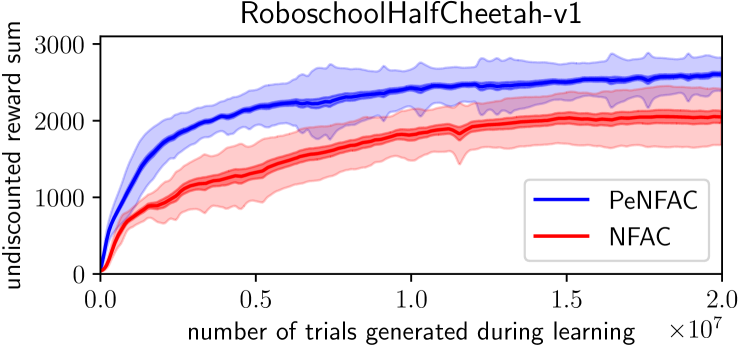
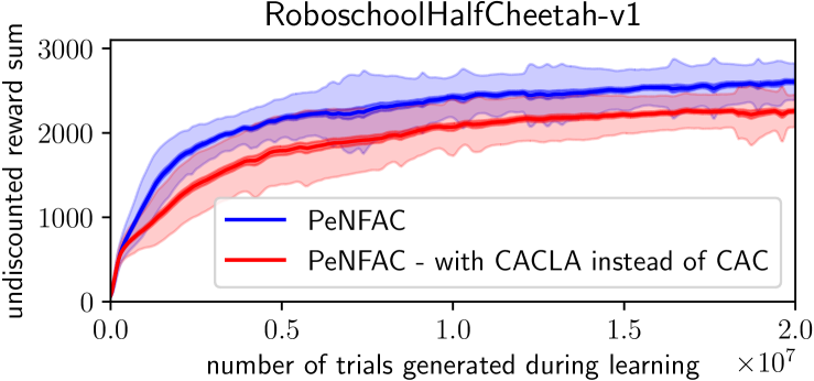
Van Hasselt and Wiering Van Hasselt and Wiering (2007) observed that the CAC update performs worse that the CACLA update in their algorithms. In their setting where the policy and the critic are updated at each timestep, we believe this observation is explained by the use of the TD error (computed from a single sample) to estimate the advantage function. However, when using variance reduction techniques such as $\lambda$-returns and learning from a batch of interactions, or when mitigating the update with a trust region constraint, we observe that this estimation becomes better (see Figure 4). This explains why we choose a CAC update in PeNFAC.

In order to ensure that $||\mu-\tilde{\mu}||_{2,\infty}$ stays small over the whole state space, we approximate it with a Euclidean norm over the state visited by $\pi$. To implement this constraint, we add a regularization term to the update and automatically adapts its coefficient, for a trajectory $(s_{0},s_{1},\ldots,s_{h})$:

$$\sum_{t=0}^{h-1}\Delta_{\text{CAC}}(s_{t},\mu_{\theta})+\beta\nabla_{\theta}\big{|}\big{|}\mu_{\text{old}}(s_{t})-\mu_{\theta}(s_{t})\big{|}\big{|}^{2}_{2},$$

where $\beta$ is a regularization coefficient. Similarly to the adaptive version of Proximal Policy Optimization (PPO) Schulman et al. (2017), $\beta$ is updated in the following way (starting from $\beta\leftarrow 1$):

• if $\hat{d}(\mu,\mu_{\text{old}})<d_{\text{target}}/1.5$: $\beta\leftarrow\beta/2$,

• if $\hat{d}(\mu,\mu_{\text{old}})>d_{\text{target}}\times 1.5$: $\beta\leftarrow\beta\times 2$,

where $\hat{d}(\mu,\mu_{\text{old}})=\frac{1}{\sqrt{mL}}\sum_{s\sim\pi}||\mu_{\text{old}}(s)-\mu_{\theta}(s)||_{2}$ with $L$ being the number of gathered states. Those hyper-parameters are usually not optimized because the learning is not too sensitive to them. The essential value to adapt for the designer is $d_{\text{target}}$. Note that the introduction of this hyperparameter mitigates the need to optimize the learning rate for the update of the policy, which is generally a much harder task.

6 Experiments

We performed two sets of experiments to answer the following questions:

1) How does PeNFAC compare with state-of-the-art algorithms for learning deterministic policies?

2) Which components of PeNFAC contribute the most to its performance?

The experiments were performed on environments with continuous state and action spaces in a time-discretized simulation. We chose to perform the experiments on OpenAI Roboschool Schulman et al. (2017), a free open-source software, which allows anyone to easily reproduce our experiments. In order to evaluate the performance of an algorithm, deterministic policies $\mu$ obtained during learning are evaluated at a constant interval during testing phases: policy $\mu$ is played in the environment without exploration. The interactions gathered during this evaluation are not available to any algorithms. The source code of the PeNFAC algorithm is available at github.com/matthieu637/ddrl. The hyperparameters used are reported in Appendix E as well as the considered range during the grid search.

6.1 Performance of PeNFAC

We compared the performance of PeNFAC to learn continuous deterministic policies with two state-of-the-art algorithms: PPO and DDPG. A comparison with NFAC is available in the ablation study (Section 6.2) and in Appendix C. Because PPO learns a stochastic policy, for the testing phases, we built a deterministic policy as follows $\mu(s)=\mathbb{E}[a|a\sim\pi_{\theta}(\cdot,s)]$. We denote this algorithm as ”deterministic PPO”. In Appendix D, we experimentally show that this does not penalize the comparison with PPO, as deterministic PPO provides better results than standard PPO. For PPO, we used the OpenAI Baseline implementation. To implement PeNFAC and compare it with NFAC, we use the DDRL library Zimmer et al. (2018). Given that DDPG is present in those two libraries, we provided the two performances for it. The OpenAI Baseline version uses an exploration in the parameter space and the DDRL version uses n-step returns.

Figure 1: Comparison of PeNFAC, DDPG and deterministic PPO over 60 different seeds for each algorithm in Hopper.

Figure 2: Comparison of PeNFAC, DDPG and deterministic PPO over 60 different seeds for each algorithm in HalfCheetah.

Figure 3: Comparison of PeNFAC, DDPG and deterministic PPO over 60 seeds for each algorithm in Humanoid.

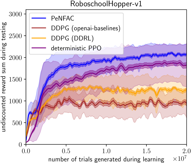
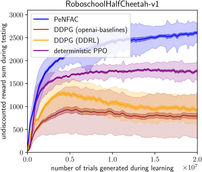
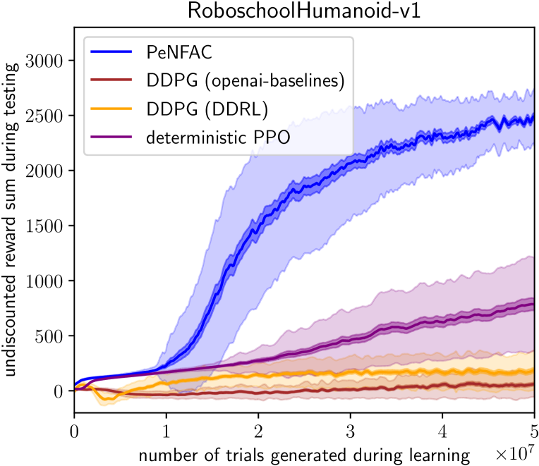
We performed learning experiments over three high-dimensional domains: Hopper, HalfCheetah and Humanoid. Dimensions of $\mathcal{S}\times\mathcal{A}$ are $15\times 3$ (Hopper), $26\times 6$ (HalfCheetah) and $44\times 17$ (Humanoid).

The neural network architecture is composed of two hidden layers of 64 units for either the policy or the value function. The choice of the activation function in the hidden units was optimized for each algorithm: we found that ReLU was better for all of them except for PPO (where tanh was better). The output activation of the critic is linear and the output activation of the actor is tanh.

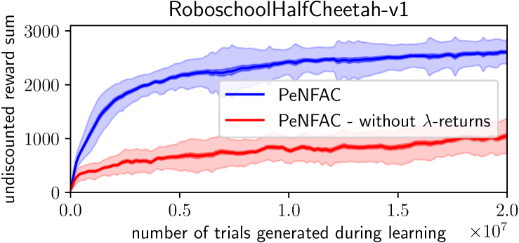
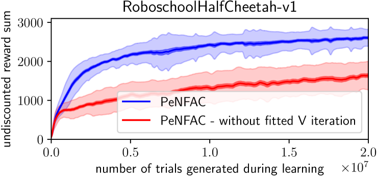
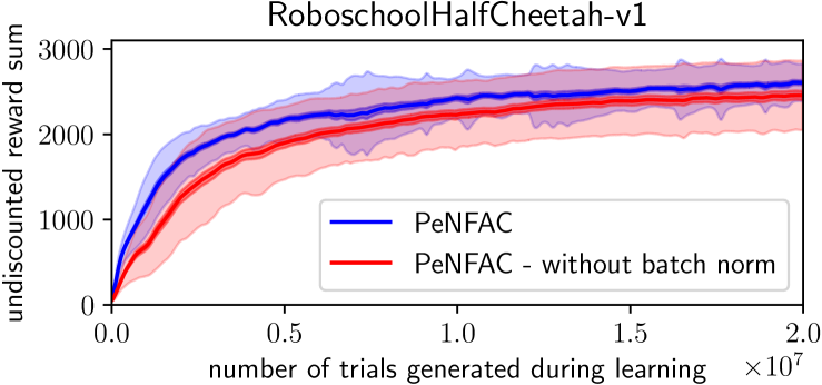
In Figures 1-4, the lighter shade depicts one standard deviation around the average, while the darker shade is the standard deviation divided by the square root of the number of seeds.

In Figures 1-3, PeNFAC outperforms DDPG and deterministic PPO during the testing phase. On Humanoid, even after optimizing the hyperparameters, we could not obtain the same results as those of Schulman et al. Schulman et al. (2017). We conjecture that this may be explained as follows: 1) the RoboschoolHumanoid moved from version 0 to 1, 2) deterministic PPO

Figure 4: Comparison of the different components ($\lambda$-returns, fitted value-iteration, CAC vs CACLA update, batch normalization) of the PeNFAC algorithm during the testing phase over the HalfCheetah environment and 60 seeds for each version.

might be less efficient than PPO, 3) neither LinearAnneal for the exploration, nor adaptive Adam step size is present in the OpenAI Baseline implementation. However, we argue that the comparison should still be fair since PeNFAC also does not use those two components. On Humanoid, we did not find a set of hyperparameters where DDPG could work correctly with both implementations.

6.2 Components of PeNFAC

In Figure 4, we present an ablation analysis in the HalfCheetah domain to understand which components of the PenFAC algorithm are the most essential to its good performance. From top to bottom plots of Figure 4, we ran PenFAC with or without trust region, with or without $\lambda$-returns, with or without fitted value iteration, with CACLA update or CAC update, and finally with or without batch normalization.

It appears that $\lambda$-returns and fitted value iteration are the most needed, while the effect of batch normalization is small and mostly helps in the beginning of the learning.

We also tried updating the actor every timestep without taking into account the sign of the advantage function (i.e., using SPG instead of CAC), but the algorithm was not able to learn at all. This also demonstrates that the CAC update is an essential component of PenFAC.

7 Conclusion

In the context of learning deterministic policies, we studied the properties of two not very well-known but efficient updates, Continuous Actor Critic Learning Automaton (CACLA) and Continuous Actor Critic (CAC). We first showed how closely they both are related to the stochastic policy gradient (SPG). We explained why they are well designed to learn continuous deterministic policies when the value function is only approximated. We also highlighted the limitations of those methods: a potential poor sample efficiency when the dimension of the action space increases and no guarantee that the underlying deterministic policy will converge toward a local optimum of $J(\mu_{\theta})$ even with a linear approximation.

In the second part, we extended Neural Fitted Actor Critic (NFAC), itself an extension of CACLA, with a trust region constraint designed for deterministic policies and proposed a new algorithm, Penalized NFAC (PeNFAC). Finally, we tried our implementation on various high-dimensional continuous environments and showed that PeNFAC performs better than DDPG and PPO to learn continuous deterministic policies.

As future work, we plan to consider off-policy learning and the combination of the updates of CAC and DPG together to ensure the convergence toward a local optimum while benefiting from the good updates of CAC.

Appendix A Proofs

A.1 Relation between DPG and CAC update for a given state

For simplification, the proof of a single dimension $k$ of the parameter space is provided. To denote the $k$^th dimension of a vector $x$, we write $x_{k}$. If $x$ is a matrix, $x_{:,k}$ represents the $k$^th column vector. We will use the following result from Silver et al. Silver et al. [2014]:

$$\lim_{\sigma\rightarrow 0}\nabla_{\theta}J(\pi_{\theta,\sigma})=\nabla_{\theta}J(\mu_{\theta}).$$

Thus, the following standard regularity conditions are required: $T,T_{0},R,\mu,\pi,\nabla_{a}T,\nabla_{a}R,\nabla_{\theta}\mu$ are continuous in all variables and bounded. From this result, we derive the following equation for a fixed state $s$:

$$\lim_{\sigma\rightarrow 0}\int_{\mathcal{A}}A^{\pi}(s,a)\nabla_{\theta}\pi_{\theta,\sigma}(a|s)da=\nabla_{a}A^{\mu}(s,a)\big{|}_{a=\mu_{\theta}(s)}\nabla_{\theta}\mu_{\theta}(s).$$

We first study the special case of $\Delta_{\text{DPG}}(s,\mu_{\theta})_{k}=0$ and want to show that ${\lim_{\sigma\rightarrow 0}\Delta_{\text{CAC}}(s,\mu_{\theta})}_{k}$ is also zero:

$${\Delta_{\text{DPG}}(s,\mu_{\theta})}_{k}=0\implies \nabla_{a}A^{\mu}(s,a)\big{|}_{a=\mu_{\theta}(s)}{\nabla_{\theta}\mu_{\theta}(s)}_{:,k}=0,$$

$$\implies \lim_{\sigma\rightarrow 0}\int_{\mathcal{A}}A^{\pi}(s,a){\nabla_{\theta}\pi_{\theta,\sigma}(a|s)}_{:,k}da=0,$$

$$\implies \lim_{\sigma\rightarrow 0}\frac{1}{\sigma^{2}}\int_{\mathcal{A}}\pi_{\theta,\sigma}(a|s)A^{\pi}(s,a)\big{(}a-\mu_{\theta}(s)\big{)}{\nabla_{\theta}\mu_{\theta}(s)}_{:,k}da=0,$$

$$\implies \lim_{\sigma\rightarrow 0}\frac{1}{\sigma^{2}}\int_{\mathcal{A}}\pi_{\theta,\sigma}(a|s)H\big{(}A^{\pi}(s,a)\big{)}A^{\pi}(s,a)\big{(}a-\mu_{\theta}(s)\big{)}{\nabla_{\theta}\mu_{\theta}(s)}_{:,k}da=0,$$

$$\implies \lim_{\sigma\rightarrow 0}{\Delta_{\text{CAC}}(s,\mu_{\theta})}_{k}=0.$$

Now, we study the more general case ${\Delta_{\text{DPG}}(s,\mu_{\theta})}_{k}\neq 0$:

$$g_{k}^{+}(s,\mu_{\theta})= \frac{\lim_{\sigma\rightarrow 0}\Delta_{\text{CAC}}(s,\mu_{\theta})_{k}}{\Delta_{\text{DPG}}(s,\mu_{\theta})_{k}},$$

$$= \frac{\lim_{\sigma\rightarrow 0}\int_{\mathcal{A}}A^{\pi}(s,a)H(A^{\pi}(s,a))\nabla_{\theta}{\pi_{\theta,\sigma}(a|s)}_{:,k}da}{\lim_{\sigma\rightarrow 0}\int_{\mathcal{A}}A^{\pi}(s,a)\nabla_{\theta}{\pi_{\theta,\sigma}(a|s)}_{:,k}da},$$

$$= \lim_{\sigma\rightarrow 0}\frac{\int_{\mathcal{A}}A^{\pi}(s,a)H(A^{\pi}(s,a))\nabla_{\theta}{\pi_{\theta,\sigma}(a|s)}_{:,k}da}{\int_{\mathcal{A}}A^{\pi}(s,a){\nabla_{\theta}\pi_{\theta,\sigma}(a|s)}_{:,k}da},$$

$$\implies 0\leq g_{k}^{+}(s,\mu_{\theta})\leq 1.$$

A.2 Performance of a deterministic policy expressed from a Gaussian stochastic policy

The proof is very similar to Kakade and Langford [2002]; Schulman et al. [2015] and easily extends to mixtures of stochastic and deterministic policies:

$$\int_{\mathcal{S}}d_{\gamma}^{\pi}(s)\int_{\mathcal{A}}\pi(a|s)A^{\mu}(s,a)dads+\int_{\mathcal{S}}d_{\gamma}^{\tilde{\mu}}(s)A^{\pi}(s,\tilde{\mu}(s))ds=$$

$$\int_{\mathcal{S}}d_{\gamma}^{\pi}(s)\int_{\mathcal{A}}\pi(a|s)\Big{(}R(s,a)+\gamma\mathbb{E}\big{[}V^{\mu}(s^{\prime})|a\big{]}-V^{\mu}(s)\Big{)}da+\int_{\mathcal{S}}d_{\gamma}^{\tilde{\mu}}(s)\Big{(}R(s,\tilde{\mu}(s))+\gamma\mathbb{E}\big{[}V^{\pi}(s^{\prime})|\tilde{\mu}(s)\big{]}-V^{\pi}(s)\Big{)}ds=$$

$$J(\pi)+J(\tilde{\mu})+\int_{\mathcal{S}}d_{\gamma}^{\pi}(s)\int_{\mathcal{A}}\pi(a|s)\Big{(}\gamma\mathbb{E}\big{[}V^{\mu}(s^{\prime})|a\big{]}-V^{\mu}(s)\Big{)}da+\int_{\mathcal{S}}d_{\gamma}^{\tilde{\mu}}(s)\Big{(}\gamma\mathbb{E}\big{[}V^{\pi}(s^{\prime})|\tilde{\mu}(s)\big{]}-V^{\pi}(s)\Big{)}ds=$$

$$J(\pi)+J(\tilde{\mu})+\int_{\mathcal{S}}d_{\gamma}^{\pi}(s)\Big{(}-V^{\mu}(s)+\gamma\int_{\mathcal{A}}\pi(a|s)\mathbb{E}\big{[}V^{\mu}(s^{\prime})|a\big{]}da\Big{)}-J(\pi)=$$

$$J(\tilde{\mu})-J(\mu).$$

A.3 Trust region for continuous deterministic policies

For this theorem we also use the following standard regularity conditions: $I(\mathcal{S})=\int_{\mathcal{S}}ds<\infty$ and $\Big{|}\Big{|}\tilde{\mu}(s)-\mu(s))\Big{|}\Big{|}_{2,\infty}<\infty$. $m$ denotes the number of dimension of the action space. We start from the two terms we want to bound:

$$\Big{|}\int_{\mathcal{S}}d^{\tilde{\mu}}_{\gamma}(s)A^{\pi}(s,\tilde{\mu}(s))-\int_{\mathcal{S}}d^{\pi}_{\gamma}(s)A^{\pi}(s,\tilde{\mu}(s))\Big{|}=$$

$$\Big{|}\int_{\mathcal{S}}\big{(}d^{\tilde{\mu}}_{\gamma}(s)-d^{\pi}_{\gamma}(s)\big{)}A^{\pi}(s,\tilde{\mu}(s))\Big{|}\leq$$

$$\int_{\mathcal{S}}\Big{|}d^{\tilde{\mu}}_{\gamma}(s)-d^{\pi}_{\gamma}(s)\Big{|}.\Big{|}A^{\pi}(s,\tilde{\mu}(s))\Big{|}\leq$$

$$\epsilon\int_{\mathcal{S}}\Big{|}d^{\tilde{\mu}}_{\gamma}(s)-d^{\pi}_{\gamma}(s)\Big{|},$$ (11)

where $\epsilon=\text{max}_{s,a}|A^{\pi}(s,a)|$.

So, we need to bound the difference between $d^{\tilde{\mu}}$ and $d^{\pi}$ for a given state $s$:

$$\Big{|}d^{\tilde{\mu}}_{\gamma}(s)-d^{\pi}_{\gamma}(s)\Big{|}=$$

$$\Big{|}\int_{\mathcal{S}}T_{0}(s_{0})\Big{(}\sum^{\infty}_{t=0}\gamma^{t}p(s|s_{0},t,\tilde{\mu})-\sum^{\infty}_{t=0}\gamma^{t}p(s|s_{0},t,\pi)\Big{)}ds_{0}\Big{|}=$$

$$\Big{|}\int_{\mathcal{S}}T_{0}(s_{0})\sum^{\infty}_{t=0}\gamma^{t}\Big{(}p(s|s_{0},t,\tilde{\mu})-p(s|s_{0},t,\pi)\Big{)}ds_{0}\Big{|}\leq$$

$$\int_{\mathcal{S}}\Big{|}T_{0}(s_{0})\Big{|}\sum^{\infty}_{t=0}\gamma^{t}\Big{|}p(s|s_{0},t,\tilde{\mu})-p(s|s_{0},t,\pi)\Big{|}ds_{0}\leq$$

$$\int_{\mathcal{S}}\sum^{\infty}_{t=0}\gamma^{t}\Big{|}p(s|s_{0},t,\tilde{\mu})-p(s|s_{0},t,\pi)\Big{|}ds_{0}\leq$$

$$\int_{\mathcal{S}}\sum^{\infty}_{t=0}\gamma^{t}\underset{t^{\prime}>0}{\operatorname{max}}\Big{|}p(s|s_{0},t^{\prime},\tilde{\mu})-p(s|s_{0},t^{\prime},\pi)\Big{|}ds_{0}=$$

$$\frac{1}{1-\gamma}\int_{\mathcal{S}}\underset{t>0}{\operatorname{max}}\Big{|}p(s|s_{0},t,\tilde{\mu})-p(s|s_{0},t,\pi)\Big{|}ds_{0}.$$ (12)

Finally, we have to bound the difference between $p(s|s_{0},t,\tilde{\mu})$ and $p(s|s_{0},t,\pi)$. To do so, we define $\tau=\{s_{1},...,s_{t}=s\}$, and $\mathcal{D}_{\tau}$ all the possible path from the state $s_{1}$ to the state $s_{t}=s$.

$$\Big{|}p(s|s_{0},t,\tilde{\mu})-p(s|s_{0},t,\pi)\Big{|}=$$

$$\Big{|}\int_{\mathcal{D}_{\tau}}\prod_{k=1}^{t}\Big{(}T(s_{k}|s_{k-1},\tilde{\mu}(s_{k-1}))-\int_{\mathcal{A}}\pi(a|s_{k-1})T(s_{k}|s_{k-1},a)da\Big{)}d\tau\Big{|}\leq$$

$$\int_{\mathcal{D}_{\tau}}\prod_{k=1}^{t}\Big{|}T(s_{k}|s_{k-1},\tilde{\mu}(s_{k-1}))-\int_{\mathcal{A}}\pi(a|s_{k-1})T(s_{k}|s_{k-1},a)da\Big{|}d\tau=$$

$$\int_{\mathcal{D}_{\tau}}\prod_{k=1}^{t}\Big{|}\int_{\mathcal{A}}\pi(a|s_{k-1})\big{(}T(s_{k}|s_{k-1},\tilde{\mu}(s_{k-1}))-T(s_{k}|s_{k-1},a)\big{)}da\Big{|}d\tau\leq$$

$$\int_{\mathcal{D}_{\tau}}\prod_{k=1}^{t}\int_{\mathcal{A}}\pi(a|s_{k-1})\Big{|}T(s_{k}|s_{k-1},\tilde{\mu}(s_{k-1}))-T(s_{k}|s_{k-1},a)\Big{|}dad\tau\leq$$

$$L\int_{\mathcal{D}_{\tau}}\prod_{k=1}^{t}\int_{\mathcal{A}}\pi(a|s_{k-1})\Big{|}\Big{|}\tilde{\mu}(s_{k-1})-a\Big{|}\Big{|}_{2}dad\tau=$$ (13)

$$L\int_{\mathcal{D}_{\tau}}\prod_{k=1}^{t}\int\frac{1}{(\sigma\sqrt{2\pi})^{m}}e^{-\frac{1}{2\sigma^{2}}||b||_{2}^{2}}\Big{|}\Big{|}\tilde{\mu}(s_{k-1})-\mu(s_{k-1})+b\Big{|}\Big{|}_{2}dbd\tau\leq$$ (14)

$$L\int_{\mathcal{D}_{\tau}}\prod_{k=1}^{t}\int\frac{1}{(\sigma\sqrt{2\pi})^{m}}e^{-\frac{1}{2\sigma^{2}}||b||_{2}^{2}}\Big{(}\Big{|}\Big{|}\tilde{\mu}(s_{k-1})-\mu(s_{k-1})\Big{|}\Big{|}_{2}+\Big{|}\Big{|}b\Big{|}\Big{|}_{2}\Big{)}dbd\tau\leq$$

$$L\int_{\mathcal{D}_{\tau}}\prod_{k=1}^{t}\Big{(}\Big{|}\Big{|}\tilde{\mu}(s_{k-1})-\mu(s_{k-1})\Big{|}\Big{|}_{2}+\int\frac{1}{(\sigma\sqrt{2\pi})^{m}}e^{-\frac{1}{2\sigma^{2}}||b||_{2}^{2}}\Big{|}\Big{|}b\Big{|}\Big{|}_{1}\Big{)}dbd\tau=$$

$$L\int_{\mathcal{D}_{\tau}}\prod_{k=1}^{t}\Big{(}\Big{|}\Big{|}\tilde{\mu}(s_{k-1})-\mu(s_{k-1})\Big{|}\Big{|}_{2}+\frac{2m\sigma}{\sqrt{2\pi}}\Big{)}d\tau\leq$$

$$L\int_{\mathcal{D}_{\tau}}\Big{(}\underset{s_{k}\in\tau}{\operatorname{max\ }}\Big{|}\Big{|}\tilde{\mu}(s_{k})-\mu(s_{k})\Big{|}\Big{|}_{2}+\frac{2m\sigma}{\sqrt{2\pi}}\Big{)}^{t}d\tau\leq$$

$$I(\mathcal{S})^{t}L\Big{(}\underset{s_{k}\in\mathcal{S}}{\operatorname{max\ }}\Big{|}\Big{|}\tilde{\mu}(s_{k})-\mu(s_{k})\Big{|}\Big{|}_{2}+\frac{2m\sigma}{\sqrt{2\pi}}\Big{)}^{t}.$$ (15)

To obtain (13), we use the assumption that the transition function is L-Lipschitz continuous with respect to the action and the L2 norm. To obtain (14), we use (5). Equation 15 does no longer depend on $s$ and $s_{0}$, thus added to (12) and (11) it gives:

$$\frac{\epsilon L}{1-\gamma}\underset{t>0}{\operatorname{max\ }}I(\mathcal{S})^{t+2}\Big{(}\Big{|}\Big{|}\tilde{\mu}(s)-\mu(s)\Big{|}\Big{|}_{2,\infty}+\frac{2m\sigma}{\sqrt{2\pi}}\Big{)}^{t}\leq$$

$$\frac{\epsilon L}{1-\gamma}\underset{t>0}{\operatorname{max\ }}\Big{(}\Big{|}\Big{|}\tilde{\mu}(s)-\mu(s)\Big{|}\Big{|}_{2,\infty}+\frac{2m\sigma}{\sqrt{2\pi}}\Big{)}^{t}.$$ (16)

To obtain (16), we suppose that $I(\mathcal{S})$ is smaller than 1. We can make this assumption without losing in generality: it would only affect the magnitude of the Lipschitz constant. Thus if $\big{|}\big{|}\tilde{\mu}(s)-\mu(s)\big{|}\big{|}_{2,\infty}+\frac{2m\sigma}{\sqrt{2\pi}}$ stays smaller than $1$, the optimal $t$ will be $1$, and (16) could be reduced to:

$$\frac{\epsilon L}{1-\gamma}\Big{(}\Big{|}\Big{|}\tilde{\mu}(s)-\mu(s)\Big{|}\Big{|}_{2,\infty}+\frac{2m\sigma}{\sqrt{2\pi}}\Big{)}.$$

Appendix B Additional experiments on CACLA’s update

In those two experiments, we want to highlight the good performance of CACLA compared to SPG and DPG without neural networks. The main argument to use DPG instead of SPG is its efficiency when the action dimensions become large. In the first experiment, we study if CACLA suffers from the same variance problem as SPG. The second experiment supports our claim that CACLA is more robust than SPG and DPG when the approximation made by the critic is less accurate.

B.1 Sensitivity to action space dimensionality

We used a setup similar to that of Silver et al. Silver et al. [2014]: those environments contain only one state and the horizon is fixed to one. They are designed such that the dimensionality of the action space can easily be controlled but there is only little bias in the critic approximation. The policy parameters are directly representing the action: $\mu_{\theta}(\cdot)=\theta$.

Compatible features are used to learn the Q value function for both SPG and DPG. For CACLA, the value function V is approximated through a single parameter. The Gaussian exploration noise and the learning rate of both the critic and actor have been optimized for each algorithm on each environment. In Figure 5, similarly to Silver et al. Silver et al. [2014], we observe that SPG is indeed more sensitive to larger action dimensions. CACLA is also sensitive to this increase in dimensionality but not as much as SPG. Finally, we also note that even if the solution of CACLA and DPG are not exactly the same theoretically, they are very similar in practice.

Figure 5: Comparison of DPG, SPG and CACLA over three domains with 100 seeds for each algorithm. On the left, the action dimensions is 5 and 50 on the right.

B.2 Robustness to the critic approximation errors

Compared to the previous experience, we introduce a bigger bias in the approximation of the critic by changing the application domains: the horizon is deeper and there is an infinite number of states. The policy is represented as $\mu_{\theta}(s)=\phi(s)\cdot\theta$ where $\phi(s)$ are tiles coding features.

Figure 6: Comparison of CACLA, DPG and SPG over two environments of OpenAI Gym and one environment of Roboschool (60 seeds are used for each algorithm).

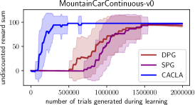
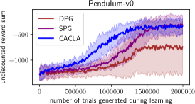
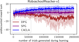
In Figure 6, we observe that as soon as value functions become harder to learn, CACLA performs better than both SPG and DPG.

Appendix C Broader comparison between PeNFAC and NFAC

To avoid overloading previous curves, we did not report the performance of NFAC (except in the ablation study on the HalfCheetah environment). In Figure 7, we extend this study to two other domains of Roboschool: Hopper and Humanoid.

Figure 7: Comparison of PeNFAC and NFAC over RoboschoolHopper and RoboschoolHumanoid with 60 seeds for each algorithm.

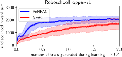
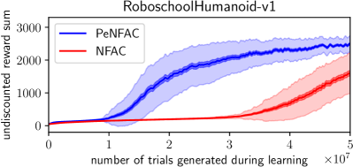
We observe that PeNFAC is significantly better than NFAC which demonstrates the efficiency of the trust region update combined with CAC.

Appendix D Impact of evaluating PPO with a deterministic policy

Figure 8: Comparison of evaluating PPO with a deterministic policy instead of the stochastic policy produced by PPO.

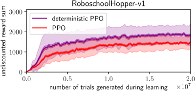
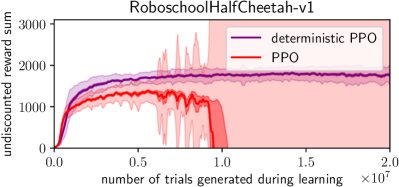
In Figure 8, we observe that using a deterministic policy to evaluate the performance of PPO is not penalizing. This is the only experiment of the paper where deterministic policies and stochastic policies are compared.

Appendix E Hyperparameters

For the sake of reproducibility Henderson et al. [2018], the hyperparameters used during the grid search are reported here. In Tables 2-5, ”ho”, ”ha” and ”hu” stand respectively for Hopper, HalfCheetah, and Humanoid Roboschool environments.

$\gamma$	$0.99$
Actor network	$64\times 64$
Critic network	$64\times 64$
Actor output activation	TanH

Table 1: Set of hyperparameters used during the training with every algorithm.

Network hidden activation	$\underset{\text{ho,ha,hu}}{\text{Leaky ReLU}(0.01)}$, TanH
Actor learning rate	$\underset{\text{ho,ha,hu}}{10^{-4}}$, $10^{-3}$, $10^{-2}$
Critic learning rate	$10^{-4}$, $\underset{\text{ho,ha,hu}}{10^{-3}}$, $10^{-2}$
Batch norm	first layer of the actor
$d_{\text{target}}$	$\underset{\text{ho,ha,hu}}{0.03}$, $0.01$, $0.005$
ADAM	$\underset{\text{ho,ha,hu}}{(0,0.999,10^{-8})}$, $(0.9,0.999,10^{-8})$
Number of ADAM iteration (actor)	10, $\underset{\text{ho,ha,hu}}{30}$, $50$
Number of ADAM iteration (critic)	1
$\lambda$	$0$, $0.5$, $0.6$, $\underset{\text{ho,ha,hu}}{0.9}$, $0.95$, $0.97$
$\sigma^{2}$ (Truncated Gaussian law)	$0.01$, $0.05$, $0.1$, $\underset{\text{ho,ha,hu}}{0.2}$, $0.5$
Number fitted iteration	$1$, $\underset{\text{ho,ha,hu}}{10}$, $20$, $50$
Update each $x$ episodes	$1$, $2$, $3$, $\underset{\text{ha}}{5}$, $10$, $\underset{\text{ho}}{15}$, $20$, $30$, $\underset{\text{hu}}{50}$, $100$

Table 2: Set of hyperparameters used during the training with PeNFAC.

Network hidden activation	$\underset{\text{ho,ha,hu}}{\text{TanH}}$, ReLu, Leaky ReLU (0.01)
Layer norm	no
ADAM	$(0.9,0.999,10^{-5})$
Entropy coefficient	0
Clip range	0.2
$\lambda$	$\underset{\text{ho,ha}}{0.97},\underset{\text{hu}}{0.95}$
Learning rate	$\underset{\text{hu}}{10^{-4}},\underset{\text{ho,ha}}{3e^{-4}}$
nminibatches	$\underset{\text{hu}}{4}$, $\underset{\text{ho,ha}}{32}$
noptepochs	$4$, $\underset{\text{ho,ha}}{10}$, $15$, $\underset{\text{hu}}{50}$
nsteps	$2^{11}$, $\underset{\text{ha}}{2^{12}}$, $\underset{\text{ho}}{2^{13}}$, $\underset{\text{hu}}{2^{14}}$, $2^{15}$, $2^{16}$
sample used to make the policy more deterministic	15

Table 3: Set of hyperparameters used during the training with PPO.

Network hidden activation	$\text{Leaky ReLU}(0.01)$
Actor learning rate	$10^{-4}$
Critic learning rate	$10^{-3}$
Batch norm	first layer of the actor
ADAM	$\underset{\text{ho,ha,hu}}{(0,0.999,10^{-8})}$, $(0.9,0.999,10^{-8})$
L2 regularization of the critic	$\underset{\text{ha,ho}}{0.01}$, $\underset{\text{hu}}{\text{without}}$
Exploration	Gaussian ($0.2$), $\underset{\text{ha,ho,hu}}{\text{Ornstein Uhlenbeck}(0.001,0.15,0.01)}$
Mini batch size	$32$, $64$, $\underset{\text{hu,ha,ho}}{128}$
Reward scale	$0.1$, $1$, $\underset{\text{hu,ha,ho}}{10}$
Soft update of target networks	$\underset{\text{hu}}{0.001}$, $\underset{\text{ha,ho}}{0.01}$
Replay memory	$10^{6}$
N-step returns	$\underset{\text{ha}}{1}$, $\underset{\text{hu,ho}}{5}$

Table 4: Set of hyperparameters used during the training with DDPG (DDRL implementation).

Network hidden activation	$\underset{\text{ho,ha,hu}}{\text{ReLu}}$, TanH
Actor learning rate	$10^{-4}$
Critic learning rate	$10^{-3}$
Layer norm	no
ADAM	$(0.9,0.999,10^{-5})$
L2 regularization of the critic	$0.01$
Exploration	Ornstein Uhlenbeck ($0.2$), $\underset{\text{ho,ha,hu}}{\text{Parameter Space (0.2)}}$
Mini batch size	$128$
Reward scale	$1$, $\underset{\text{ho,ha,hu}}{10}$
Soft update of target networks	$\underset{\text{ho,hu}}{0.001}$, $\underset{\text{ha}}{0.01}$
Replay memory	$10^{6}$
nb_rollout_steps	$10$,$\underset{\text{ho,ha,hu}}{100}$
nb_train_steps	$1$,$10$,$\underset{\text{ho,ha,hu}}{50}$

Table 5: Set of hyperparameters used during the training with DDPG (OpenAI baselines implementation).

References

- Colas et al. [2018] Cédric Colas, Olivier Sigaud, and Pierre-Yves Oudeyer. GEP-PG: Decoupling Exploration and Exploitation in Deep Reinforcement Learning Algorithms. In International Conference on Machine Learning (ICML), Stockholm, Sweden, July 2018.
- Henderson et al. [2018] Peter Henderson, Riashat Islam, Philip Bachman, Joelle Pineau, Doina Precup, and David Meger. Deep reinforcement learning that matters. In Thirty-Second AAAI Conference on Artificial Intelligence, 2018.
- Ioffe and Szegedy [2015] Sergey Ioffe and Christian Szegedy. Batch Normalization: Accelerating Deep Network Training by Reducing Internal Covariate Shift. arXiv preprint arXiv:1502.03167, 2015.
- Kakade and Langford [2002] Sham Kakade and John Langford. Approximately optimal approximate reinforcement learning. In ICML, volume 2, pages 267–274, 2002.
- Kingma and Ba [2015] Diederik P. Kingma and Jimmy L. Ba. Adam: a Method for Stochastic Optimization. International Conference on Learning Representations, pages 1–13, 2015.
- Konda and Tsitsiklis [1999] Vijay R. Konda and John N. Tsitsiklis. Actor-Critic Algorithms. Neural Information Processing Systems, 13:1008–1014, 1999.
- Lillicrap et al. [2016] Timothy P. Lillicrap, Jonathan J. Hunt, Alexander Pritzel, Nicolas Heess, Tom Erez, Yuval Tassa, David Silver, and Daan Wierstra. Continuous control with deep reinforcement learning. ICLR, 2016.
- Matyas [1965] J Matyas. Random optimization. Automation and Remote control, 26(2):246–253, 1965.
- Mnih et al. [2015] Volodymyr Mnih, Koray Kavukcuoglu, David Silver, Andrei a Rusu, Joel Veness, Marc G. Bellemare, Alex Graves, Martin Riedmiller, Andreas K. Fidjeland, Georg Ostrovski, Stig Petersen, Charles Beattie, Amir Sadik, Ioannis Antonoglou, Helen King, Dharshan Kumaran, Daan Wierstra, Shane Legg, and Demis Hassabis. Human-level control through deep reinforcement learning. Nature, 518(7540):529–533, 2015.
- Prokhorov and Wunsch [1997] Danil V. Prokhorov and Donald C. Wunsch. Adaptive critic designs. IEEE Transactions on Neural Networks, 8(5):997–1007, 1997.
- Schulman et al. [2015] John Schulman, Sergey Levine, Michael Jordan, and Pieter Abbeel. Trust Region Policy Optimization. International Conference on Machine Learning, page 16, 2015.
- Schulman et al. [2017] John Schulman, Filip Wolski, Prafulla Dhariwal, Alec Radford, and Oleg Klimov. Proximal policy optimization algorithms. CoRR, abs/1707.06347, 2017.
- Silver et al. [2014] David Silver, Guy Lever, Nicolas Heess, Thomas Degris, Daan Wierstra, and Martin Riedmiller. Deterministic Policy Gradient Algorithms. Proceedings of the 31st International Conference on Machine Learning, pages 387–395, 2014.
- Smith [2005] Russell Smith. Open dynamics engine. 2005.
- Sutton et al. [1999] Richard S. Sutton, David Mcallester, Satinder Singh, and Yishay Mansour. Policy Gradient Methods for Reinforcement Learning with Function Approximation. In Advances in Neural Information Processing Systems 12, pages 1057–1063, 1999.
- Sutton [1988] Richard S. Sutton. Learning to predict by the methods of temporal differences. Machine learning, 3(1):9–44, 1988.
- Van Hasselt and Wiering [2007] Hado Van Hasselt and Marco A. Wiering. Reinforcement learning in continuous action spaces. In Proceedings of the IEEE Symposium on Approximate Dynamic Programming and Reinforcement Learning, pages 272–279, 2007.
- Zimmer et al. [2016] Matthieu Zimmer, Yann Boniface, and Alain Dutech. Neural Fitted Actor-Critic. In European Symposium on Artificial Neural Networks, Computational Intelligence and Machine Learning, 2016.
- Zimmer et al. [2018] Matthieu Zimmer, Yann Boniface, and Alain Dutech. Developmental reinforcement learning through sensorimotor space enlargement. In The 8th Joint IEEE International Conference on Development and Learning and on Epigenetic Robotics, September 2018.