Identification of taxon through classification with partial reject options

Abstract

Identification of taxa can significantly be assisted by statistical classification based on trait measurements in two major ways; either individually or by phylogenetic (clustering) methods. In this paper we present a general Bayesian approach for classifying species individually based on measurements of a mixture of continuous and ordinal traits as well as any type of covariates. It is assumed that the trait vector is derived from a latent variable with a multivariate Gaussian distribution. Decision rules based on supervised learning are presented that estimate model parameters through blockwise Gibbs sampling. These decision regions allow for uncertainty (partial rejection), so that not necessarily one specific category (taxon) is output when new subjects are classified, but rather a set of categories including the most probable taxa. This type of discriminant analysis employs reward functions with a set-valued input argument, so that an optimal Bayes classifier can be defined. We also present a way of safeguarding against outlying new observations, using an analogue of a $p$-value within our Bayesian setting. Our method is illustrated on an original ornithological data set of birds. We also incorporate model selection through cross-validation, examplified on another original data set of birds.

1 Introduction

1.1 Biological taxonomy

Biological taxonomy relies on correct classification of organisms to taxa, which in turn requires that reliable and detailed data is available to learn the decision rules. The use of traits to numerically classify taxa has a long history, cf. Sneath and Sokal (1973); Barnett et al. (1979); Payne and Preece (1980); Felsenstein (1983) for a summary of early work. These traits are either morphological or genetic, and measured on a scale that is either continuous, ordinal or categorical, or a mixture of these. In order to classify new organisms, some kind of reference material (or a training data set) is needed, to which the trait vector of the new subject is compared and matched. This requires that supervised learning or discriminant analysis has been applied to training data in order to generate a decision rule, so that the new organisms can be assigned to the taxon whose decision region includes this subject’s trait vector. Such a classifier is either phylogenetic or individual, depending on whether genetic relationships between species are taken into account or not when the decision regions are derived. For instance, in the context of bacterial classification, Wang et al. (2007) introduce an individual (naive Bayesian) classifier, whereas Gao et al. (2017) define a phylogenetic classifier such that when multiple taxa of the reference material match the trait vector of a new observation, information from a phylogenetic tree (Huelsenbeck and Ronquist, 2001) is used in order to facilitate classification.

Population ecology and ornithology in particular are important applications of biological taxonomy. To the authors’ knowledge, there has been no published interpretable and general approach to classifying ornithological data. The widely used work of Svensson (1992) in bird species identification makes rich use of numerical combinations (often refered to as “wing formulae”) of trait observations to classify birds to taxa, but offers no general solution. Modern approaches to bird species classification include the Merlin Bird ID software, by the Cornell Lab of Ornithology. Merlin Bird ID uses convolutional neural networks for image recognition (LeCun et al., 1989) and gives the user a ranked list of species to choose from. Due to the machine learning approach parameter interpretability is complicated though, and not accessible to the user.

1.2 Unsupervised learning

A number of unsupervised leaning methods methods have been proposed, as summarized for instance in Ripley (1996); Hastie et al. (2009); Liu et al. (2011). For continuous traits this includes linear (or Fisher) discriminant analysis (LDA, Fisher, 1936), quadratic discriminant analysis (QDA, Smith, 1946; Bensmail and Celeux, 1996; Fraley and Raftery, 2002), heteroscedastic discriminant analysis (Kumar and Andreou, 1998), regularized discriminant analysis (Friedman, 1989), mixture discriminant analysis (Hastie and Tibshirani, 1996), and probabilistic Fisher discriminant analysis (Bouveyron and Brunet, 2012). These are all soft discrimination methods (Wahba, 1998), where a joint statistical distribution of class membership (taxon) and trait is assumed, and the class with maximal posterior probability is selected. Bayes’ rule is used to compute the posterior probabilities in terms of prior probabilities of classes and the likelihoods of trait vectors conditional on classes. In particular, a naive Bayes classifier corresponds to a model for which the trait vectors are conditionally independent conditional on class (Domingos and Pazzani, 1997). Logistic regression and penalized logistic regression (Lin et al., 2000) can also be used for soft binary classification by specifying the posterior probabilities directly in terms of a regression model, with traits as covariates. In particular, this makes it easy to incorporate continuous as well as categorical traits. For any of the abovementioned soft classifiers, if the parameters of the likelihood are random as well, the resulting method is an instance of predictive classification or Bayesian discriminant analysis (Section 2.4 of Ripley, 1996; Aitchison and Dunsmore, 1980; Geisser, 1993; Hjort, 1986). This includes, for instance, the Bayesian version of QDA (Geisser, 1964; Fraley and Raftery, 2007). On the other hand, many machine learning methods, such as support vector machines (Cortes and Vapnik, 1995), distance-weighted discrimination (Marron et al., 2007), and boosting (Friedman et al., 2000), require no statistical model at all, since the decision regions of the classifier are defined in terms of an algorithm that does not rely on any model for how data was generated.

As mentioned above, it is often the case that taxonomic data is a mixture of various types of observations (continuous, integer valued, ordered categorical). For instance, there might be partial observations (due to e.g. rounding or grouping) or some components of the trait vector might be missing. Models for mixed type of data are important for a wide range of applications (De Leon and Chough, 2013). Here we will use the umbrella term obfuscated observations for partial and missing observations among the components of the trait vector. A general way to handle obfuscated data is to define a distance between pairs of trait vectors, and then employ a nearest neighbour method for classfication (Gower, 1971; Gower and Legendre, 1986; Kauffmann and Rousseeuw, 1990; D’Orazio, 2021). Another option for mixed data is to use a model-based soft classifier, with latent multivariate Gaussian variables, whose components are suiably obfuscated in order to generate the observed trait vector. These types of models have been used in Item Response Theory (IRT), originally proposed by Thurstone (1925) in the context of ecudational testing. The theory has since then been developed by many authors (Lord, 1952; Rasch, 1993; Vermunt, 2001; Lord and Novick, 2008). More recent Bayesian models of categorical data include Albert and Chib (1993); Fokoué and Titterington (2003); Chu and Ghahramani (2005); McParland et al. (2014, 2017). Another Bayesian soft classifier for ordinal data, a mixed membership model with a gamma distributed hidden variable, has been proposed by Virtanen and Girolami (2015).

It is often the case that two or more taxa fit the new observation almost equally well. It is possible then to include a reject option of the classifier that corresponds to “don’t know”. Binary classfication with reject options has been studied by Chow (1970) and Herbei and Wegkamp (2006) (see also Freund et al. (2004)), whereas Ripley (1996) adds a reject option for discrimination between an arbitrary number of classes. In taxonomy it is also important to provide some kind of cutoff when none of the candidate taxa fit the trait vector of the new organism well. This is achieved, for model-based soft classifiers, by declaring the newly observed trait vector as an outlier when its $p$-value is smaller than a cutoff. This $p$-value is based on a measure of oytlyingness of the observed new trait vector, using the mixture distribution of traits from training data of all classes as the analogue of a null distribution (Ripley, 1996).

1.3 The present article

The classification method presented in this paper is a generalization of the approaches suggested in Svensson (1992) and Malmhagen et al. (2013). We develop a method that makes it possible to conclude which trait measurements that characterize various taxa, as an alternative to neural networks and other black box methods. Our method can be viewed as an extension of Bayesian QDA that incorporates traits of mixed types, which are components of a hidden Gaussian vector that have been obfuscated in order to obtain the observed trait vector. In particular we draw on work by Albert and Chib (1993); Fokoué and Titterington (2003); McParland et al. (2014, 2017) and defined a Bayesian classifier whose parameters are estimated from training data by means of blockwise Gibbs sampling (Geman and Geman, 1984; Robert and Casella, 2013). The inclusion of covariates is mentioned as an extension in the discussion sections of McParland et al. (2014, 2017). Here we contribute to this extension, assuming that the location as well as the scale parameter of the latent Gaussian distribution depend on covariates, so that heteroscedasticity is achieved. We believe this covariate extension is important, since taxonomic trait measurments of population ecology data is usually informative conditional on other information. In other words, the same value of a trait measurement might indicate different taxa for a subject, depending on the particular subject’s additional information. In order to control for this additional information, we include it as set of covariates, and construct our classifier conditional on the covariate information for each subject.

A major novelty of our work is the use of set-valued outputs of the classifier. A set of size 0 corresponds to a scenario where no taxon fits the new organism (an outlier), a set of size 1 corresponds the case where one taxon fits the new organism better than all the others, whereas a set of size $N$, where $N$ is the number of classes, corresponds to a reject option. We also allow for decision regions with $2,\ldots,N-1$ species, corresponding to a partial reject option, where no single species is chosen, but some are excluded. In this way we generalize work by Chow (1970); Ripley (1996); Freund et al. (2004); Herbei and Wegkamp (2006), making use of a reward function with a set-valued input argument, so that an associated set-valued Bayesian classifier is defined. In order to handle outlying trait vectors, in contrast to Ripley (1996), a new organism’s trait vector is assigned one $p$-value for each taxon, rather than one single $p$-value for the whole training data set.

The primary scenario for which we envision use of our proposed method is as follows: A researcher has a desire to construct a procedure to classify subjects into a, usually small, number of taxa. The procedure should not require any advanced or expensive technology, but rather be viable using only visual observations or simple measurements from everyday tools, such as rulers, callipers and scales. Such a procedure has the potential to aid data collection for population ecologists, if high requirements on classification correctness are met. It is assumed that the researcher has access to training data where each subject has a know taxon, and the traits shared by the taxa are observed for the subjects, although not neccessarily perfectly. To achieve this goal, the researcher would apply our proposed methodology and, if feasible, derive a comprehensive list of which trait observations that signify the various taxa, and which are ambiguous. In short, the goal is to specify a decision rule that is not black box, which will be feasible when the number of traits is small.

The secondary scenario for using our methodology is that in which an agent desires to classify an organism to a taxon, but is unable to do so without some kind of aid. This could be due to inexperience of the considered taxa, or because the number of traits and the number of different outcomes of the traits are too large to extract a decision rule that is nimble. In such a situation, our method can provide tailored prediction of a taxon given the observed traits.

Our paper is organized as follows. In Section 2 we present the application with original ornithological data, which will be employed as we present and analyze our method of classification. The core models, multivariate and multiple regression with Gaussian errors for perfectly observed data, and the corresponding latent Gaussian models for obfuscated data, are presented in Section 3 in general but concise terms, and specified for our type of data. Section 4 presents soft (posterior probability) classification in conjunction with reward functions with set-valued input arguments. In Section 5 we propose model selection (both for traits and covariates) through cross-validation and apply it on another original data set. A comparison with mclust (Scrucca et al., 2016), the most popular R-package for clustering and classification using discriminant analysis, is made in Section 6. Section 7 contains the discussion. Most of the mathematical details are placed in the appendices, and we will refer to them accordingly.

As a final note, we stress that the presented approach in no way is limited to population ecology data and classification of subjects to taxa. It is applicable more generally for classification with partial reject options, of traits vectors whose components might be a mixture of different types.

2 Bird species classification

In order to showcase in detail the use of our method, we will present an example of bird species classification using an original data set A minor subset of this primary data set was used in Walinder et al. (1988) and Malmhagen et al. (2013), but the data set as a whole is unpublished. We will also make use of a second original, unpublished data set in Section 5, the details of which we present in that section. Both data sets were collected by the Falsterbo Bird Observatory.

The primary data set concerns four morphologically similar warblers in the Acrocephalus genus; Eurasian Reed Warbler (Acrocephalus scirpaceus), Marsh Warbler (Acrocephalus palustris), Blyth’s Reed Warbler (Acrocephalus dumetorum) and Paddyfield Warbler (Acrocephalus agricola). They constitute a typical example of species that experts with long experience can classify through visual observation, whereas those with less experience usually need measurements of particular traits to aid their classification. Our material contains measurements of these traits for birds that have been identified by experts.

Data was collected from wild birds captured and ringed in Falsterbo, Sweden, and from museum specimens at the museums of natural history in Stockholm, Copenhagen, and Tring. All birds have three traits of main concern, the wing length (measured as described in Svensson, 1992), the notch length of feather P2 (measured as described in Figure 1 of Malmhagen et al., 2013) and the relative position of the P2 notch to the rest of the wing, referred to as the notch position (taken as described in Svensson, 1992). These are all measurements of different parts of the wing. The only covariate is age, and it is binary, with levels juvenile and adult. Age is included as a covariate due to a suspected change in the trait distribution (both location and scale) between the birds’ juvenile and adult plumages.

Ideally, wing length and notch length are measured continuously, but in reality this is impossible. Instead, wing length is rounded to integer millimeters, as this is the typical unit that gives consistent measurements. By the same rationale notch length is rounded to half millimeters. Finally, notch position is by definition ordered categorical. It measures where in relation to the other wing feathers the notch is positioned and it is defined as the feather closest to the notch.

Overall we have 54 155 observed birds, and these constitute the referential data for this classification problem. These are distributed as presented in Table 1. The uneven distribution of observations across taxa will be commented on throughout the analysis of the data set.

Table 1: The distribution of the Acrocephalus data over species, covariates and traits. Note that the Paddyfield Warbler has few observations overall, but almost all of them are complete, whereas the Reed Warbler has many observations but only a small percentage of them are complete.

		Species
Trait	Covariate	Reed W.	Blyth’s Reed W.	Paddyfield W.	Marsh W.
Wing	Juvenile	36 023	41	19	2 534
length	Adult	14 536	68	12	870
Notch	Juvenile	830	41	18	2 212
length	Adult	472	68	12	579
Notch	Juvenile	410	41	19	416
Position	Adult	77	68	12	40

3 Model formulation

We will first present the model for the case where all trait measurements are continuous and perfectly observed and thereafter for the case where the vector of trait measurements are obfuscated in different ways, including missing values.

3.1 Ideal case; no obfuscated trait measurements

Suppose we have $N$ different categories (or classes), contained in the set $\mathsf{N}=\{1,\ldots,N\}$, with known prior probabilities $\pi=(\pi_{1},\ldots,\pi_{N})$. With full data we measure $q$ traits and $p$ covariates of each subject. Let $Y_{ijk}$ be the measurement of trait $k$ for subject $j$ in category $i$, where $1\leq i\leq N$, $1\leq j\leq n_{i}$, $1\leq k\leq q$ and $n_{i}$ is the number of subjects in category $i$. We assume that

$$Y_{ij}=(Y_{ij1},\ldots,Y_{ijq})\sim\text{N}\left(m_{ij},\mathbf{\Sigma}_{ij}\right)$$ (1)

are independent random vectors, each one having a multivariate normal distribution, with

$$m_{ij}=(m_{ij1},\ldots,m_{ijq})\qquad\text{and}\qquad\mathbf{\Sigma}_{ij}=\left(\Sigma_{ijkl}\right)_{k,l=1}^{q}$$

being the mean vector and the covariance matrix of subject $j$ of category $i$. The Gaussian assumption on $Y_{ij}$ is especially suitable when the inheritable components of the traits are known to be or can be assumed to be of polygenic nature and the environmental influence on the traits consists of many factors, each with a small effect. This is commonly the case for traits such as height or color of body parts (Lynch and Walsh, 1998; Lande et al., 2003). Let also

$$x_{ij}=\left(1,x_{ij1},\ldots,x_{ijp}\right)=\left(x_{ijm}\right)_{m=0}^{p}$$

be the covariate vector of subject $j$ of category $i$. Trait vectors and covariate vectors of category $i$ are rows in the matrices $\mathbf{Y}_{i}=\left(Y_{i1}^{\top},\ldots,Y_{in_{i}}^{\top}\right)^{\top}$ and $\mathbf{X}_{i}=\left(x_{i1}^{\top},\ldots,x_{in_{i}}^{\top}\right)^{\top}$ respectively, where $\top$ refers to matrix transposition. We now proceed by formulating a multivariate and multiple regression model

$$\mathbf{Y}_{i}=\mathbf{X}_{i}\mathbf{B}_{i}+\mathbf{E}_{i}$$ (2)

for category $i$, where $\mathbf{B}_{i}=\left(B_{imk};m=0,\ldots,p;k=1,\ldots,q\right)$ is the regression parameter matrix, whose first row consists of intercepts for the $q$ traits, $m_{ij}$ is the $j^{\text{th}}$ row of $\mathbf{X}_{i}\mathbf{B}_{i}$, and $\mathbf{E}_{i}=\left(E_{i1}^{\top},\ldots,E_{in_{i}}^{\top}\right)^{\top}$ is an error term matrix with independent rows $E_{ij}\sim\text{N}(0,\mathbf{\mathbf{\Sigma}}_{ij})$.

For use in the construction of a joint prior, and later the derivation of the marginal posterior distributions of the parameters, the vectorized form of our regression model is needed. Denote by $\mbox{vec}(\cdot)$ the vectorization operation of a matrix, that appends the columns of the matrix from left to right on top of each other (Macedo and Oliveira, 2013). The inverse of the vec operation will also be used, and it is denoted by $\mbox{vec}^{-1}(\cdot)$. Then rewrite (2) as

$$\mathbf{U}_{i}=\text{vec}(\mathbf{Y}_{i})=\mathbf{Z}_{i}\beta_{i}+\text{vec}(\mathbf{E}_{i})$$ (3)

with $\beta_{i}=\text{vec}(\mathbf{B}_{i})$. Denoting an identity matrix of rank $q$ with $\mathbf{I}_{q}$ and using the matrix tensor (or Kronecker) product $\otimes$,

$$\mathbf{Z}_{i}=\mathbf{I}_{q}\otimes\mathbf{X}_{i}=\begin{pmatrix}\mathbf{X}_{i}&0&\cdots&0\\ 0&\mathbf{X}_{i}&\ddots&\vdots\\ \vdots&\ddots&\ddots&0\\ 0&\cdots&0&\mathbf{X}_{i}\end{pmatrix}$$ (4)

is a block-diagonal matrix with $q$ blocks along the diagonal.

Now suppose we have $A$ covariance classes $\alpha=1,\ldots,A$ for category $i$ such that

$$\mathbf{\Sigma}_{ij}=\mathbf{\Sigma}^{\alpha}_{i}\quad\text{if }x_{ij}\in\mathcal{X}^{\alpha},$$ (5)

where $\mathcal{X}=\mathcal{X}^{1}\cup\ldots\cup\mathcal{X}^{A}$ is a disjoint decomposition of the predictor space $\mathcal{X}$. Assume a prior $\text{N}\left(\left(b_{i0k},\ldots,b_{ipk}\right)^{\top}=b_{ik},\mathbf{\Sigma}_{\mathbf{B}_{i}}\right)$ on each of the columns $k=1,\ldots,q$ of $\mathbf{B}_{i}$. This implies a prior $\text{N}\left(\left(b_{i1}^{\top},\ldots,b_{iq}^{\top}\right)^{\top}=\beta_{i0},\mathbf{I}_{q}\otimes\mathbf{\Sigma}_{\mathbf{B}_{i}}=\mathbf{\Sigma}_{\beta_{i}}\right)$ on $\beta_{i}$. Further, assuming prior independence and imposing an Inverse-Wishart distribution $\mathbf{\Sigma}_{i}^{\alpha}\sim IW(\nu_{0},\mathbf{V}_{0})$ (see for instance Gelman et al. (2013)) on the covariance matrices in (5) for $\alpha=1,\ldots,A$, we get the joint prior

$$p(\beta_{i},\mathbf{\Sigma}_{i}^{1},\ldots,\mathbf{\Sigma}_{i}^{A})=p(\beta_{i})\prod_{\alpha=1}^{A}p(\mathbf{\Sigma}_{i}^{\alpha})$$ (6)

for the parameters of category $i$.

Write ${\cal D}_{i}=(\mathbf{X}_{i},\mathbf{Y}_{i})$ for the training data of category $i$ and let $(x,Y)$ be a new obervation that we want to classify. The predictive classifier in Section 4 will involve the density $\omega_{i}=f(Y;x|{\cal D}_{i})=\mathbb{E}[f(Y;x,\theta_{i}|{\cal D}_{i})]$ of this new observation, in case it belongs to category $i$, where $f(Y;x,\theta_{i})$ is the density function of the trait vector $Y$ conditional on the covariate vector $x$ and the parameter vector $\theta_{i}$. For a detailed derivation of the collection of model parameters $\theta_{i}=\left(\mathbf{B}_{i},\mathbf{\Sigma}^{1}_{i},\ldots,\mathbf{\Sigma}_{i}^{A}\right)$ and the posterior category weights $(\omega_{1},\ldots,\omega_{N})$ we refer to Appendix A. The Monte Carlo approximations of $\theta_{i}$ and $\omega_{i}$, $i\in\mathsf{N}$ are

$$\hat{\theta}^{\text{(Bayes)}}_{i}=\frac{1}{R_{i}}\sum_{r=1}^{R_{i}}\theta_{ir}$$ (7)

and

$$\hat{\omega}_{i}=\frac{1}{R_{i}}\sum_{r=1}^{R_{i}}f(Y;x,\theta_{ir})$$ (8)

respectively, where $R_{i}$ is the number of samples drawn from the posterior distribution of $\theta_{i}$, with $\theta_{ir}$ the parameter vector obtained by blockwise Gibbs sampling (Geman and Geman, 1984; Robert and Casella, 2013) in simulation run $r$.

3.2 General case; all types of obfuscation may occur

Overall our setup is the same as in Section 3.1, but now we suppose there is only partial information about the complete training data set ${\cal D}=\{(\mathbf{X}_{i},\mathbf{Y}_{i});\,i=1,\ldots,N\}$. Due to some obfuscation, which could be due to rounding, grouping, categorization or lost measurements of some traits, we typically have a mixture of different types of observations (De Leon and Chough, 2013) and only know that

$$Y_{ij}\in\mathsf{S}_{ij}=\mathsf{S}_{ij1}\times\cdots\times\mathsf{S}_{ijq},$$ (9)

i.e. the complete trait vector $Y_{ij}$ for subject $j$ of category $i$ is contained in a hyperrectangle $\mathsf{S}_{ij}$, whose components are given by $\{\mathsf{S}_{ijk}\}_{k=1}^{q}$. These components are sets, ranging in possible size from singletons to infinite intervals of $\mathbb{R}$, and they are given by

$$\mathsf{S}_{ijk}=\begin{cases}Y_{ijk},&k\notin\mathsf{K}_{ij},\\ \left(c_{ijk},d_{ijk}\right],&k\in\mathsf{K}_{ij},\end{cases}$$ (10)

where $\mathsf{K}_{ij}=\left\{k;1\leq k\leq q;\,Y_{ijk}\text{ obfuscated}\right\}$. The obfuscations in (9)-(10) are of the same type as in IRT (Lord and Novick, 2008; Fox, 2010). The main difference is that the covariance matrix of the trait vector $Y_{ij}$ in (1) is arbitrary, whereas the covariance matrix of IRT models typically have a factor analysis structure (Spearman, 1904), so called mixture of factor analysis models for mixed data (MFA-MD; McParland et al., 2017).

More specifically, the obfuscations in (9)-(10) are of three main types. First, if a trait $Y_{ijk}$ is unobserved, written as $Y_{ijk}=\texttt{NA}$, the $k$:th component of $\mathsf{S}_{ij}$ is of infinite length; e.g. $c_{ijk}=-\infty$, $d_{ijk}=\infty$, and we let the interval be open. That is, the interval $\mathsf{S}_{ijk}$ equals $\mathbb{R}$. Secondly, a trait may be obfuscated in such a way that interval limits are observed. Rounding is a typical example of this; consider a measurement of a trait $y_{ijk}\in\mathbb{R}^{+}$ that has been rounded to $z_{ijk}\in 2\tau\cdot\mathbb{Z}^{+}$. We put $c_{ijk}=z_{ijk}-\tau$ and $d_{ijk}=z_{ijk}+\tau$, which constitute the limits of the interval around $z_{ijk}$. Generally, we assume rounding to the midpoint of an interval. We can always scale so that the interval is of unit length, which would be equivalent to $\tau=1/2$. Lastly we have the case when we observe an ordered categorical random variable $Z_{ijk}$. We assume there is an underlying normally distributed variable $Y_{ijk}$, and that each category $z_{ijk}$ corresponds to an interval of possible values of $y_{ijk}$. Count data can be treated as an instance of this type of obfuscation, for instance traits that represent the number of occurrences of something.

We will treat all types of obfuscations in the following unified way. Suppose trait $k$ of subject $j$ of category $i$ is imperfectly observed, i.e. $k\in\mathsf{K}_{ij}$. Let $g_{k}$ be the number of categories of this trait, which we number as $0,1,\ldots,g_{k}-1$. The observed category is $z_{ijk}\in\left\{0,1,\ldots,g_{k}-1\right\}$, where $g_{k}=2$ for binary data and $g_{k}=\infty$ for count data. The corresponding side of $\mathsf{S}_{ij}$ is

$$\mathsf{S}_{ijk}=\begin{cases}\left(-\infty,\frac{1}{2}\right],&\text{if }z_{ijk}=0,\\ \left(z_{ijk}-\frac{1}{2},z_{ijk}+\frac{1}{2}\right],&\text{if }1\leq z_{ijk}\leq g_{k}-2,\\ \left(g_{k}-\frac{3}{2},\infty\right),&\text{if }z_{ijk}=g_{k}-1.\end{cases}$$

Here, a useful trick would be to add auxiliary categories, that never were observed, to take the place of $z_{ijk}=0$ and $z_{ijk}=g_{k}-1$. That ensures all observed intervals are of unit length, although we may let intervals vary in length if there is reason to construct such a model. We also write

$$Z_{ijk}=z(\mathsf{S}_{ijk})=\begin{cases}0,&\text{if }\mathsf{S}_{ijk}=\left(-\infty,\frac{1}{2}\right],\\ \frac{c_{ijk}+d_{ijk}}{2},&\text{if $\mathsf{S}_{ijk}$ is bounded},\\ g_{k}-1,&\text{if }\mathsf{S}_{ijk}=\left(g_{k}-\frac{3}{2},\infty\right],\end{cases}$$

for the center point of a finite or half-open and infinite $\mathsf{S}_{ijk}$, whereas $Z_{ijk}=z\left(\mathsf{S}_{ijk}\right)=Y_{ijk}$ when $Y_{ijk}=\mathsf{S}_{ijk}$ is perfectly observed. We will write the observed training data set as

$${\cal D}^{\text{obs}}=\left\{\left(x_{ij},\mathsf{S}_{ij}\right);\,i=1,\ldots,N,j=1,\ldots,n_{i}\right\}.$$

Finally, we remark on the importance (or lack thereof) of taking rounding into account. Consider rounding a Gaussian trait $Y_{ijk}$ to $z_{ijk}\in\mathbb{Z}$ for some $k$, $i=1,\ldots,N$ and $j=1,\ldots,n_{i}$. Suppose we have no covariates and that $Y_{ijk}\sim N(m_{ik},\sigma_{ik}^{2})$ for $j=1,\ldots,n_{i}$. An unbiased estimator of $m_{ik}$ is the average $\bar{Y}_{ik}$, whereas $\bar{Z}_{ik}$ is a biased estimator of $m_{ik}$. It is possible to quantify the size of the bias using $\sigma_{k}$ and the width of the rouding interval $\mathsf{w}=\eta_{k}\sigma_{k}$ (Tricker, 1984). In short, the larger $\mathsf{w}$ is relative to $\sigma_{k}$, the larger the bias is, as measured by $\eta_{k}$. Already when $\sigma_{k}=\mathsf{w}=1$, the bias is very small, and hence, unless an extremely precise mean estimate is needed, the bias is small compared to the uncertainty of the parameter estimate. Therefore, one might regard rounded values as true values, if the standard deviation of the trait that is rounded, is large enough.

Let $(x,\mathsf{S})$ refer to a new observation, for which the trait vector $Y\in\mathsf{S}$ is obfuscated for traits $k\in\mathsf{K}$. We refer to Appendices B and C for full details on the derivation of exact estimators of the model parameters $\theta_{i}$ and posterior weights $\omega_{i}=\mathbb{P}(\mathsf{S};x\mid\mathcal{D}_{i}^{\text{obs}})$ of category $i$, as well as Monte Carlo approximtions thereof. In brief, for each category $i$ we want to generate the set

$$\left\{\theta_{ir},Y_{ijkr},\,1\leq j\leq n_{i},\,k\in\mathsf{K}_{ij};Y_{kr},k\in\mathsf{K}\right\}_{r=1}^{R_{i}}$$ (11)

of $R_{i}$ blockwise Gibbs sampling iterates from the joint density

$$p(\theta_{i}|{\cal D}^{\text{obs}}_{i})\prod_{j=1}^{n_{i}}f\left(y_{ij\mathsf{K}_{ij}}\mid x_{ij},\mathsf{S}_{ij},\theta_{i}\right)f\left(y_{\mathsf{K}}\mid x,Y_{\mathsf{K}^{\complement}};\theta_{i}\right)$$ (12)

of the parameters $\theta_{i}$, the imperfectly observed training data and the imperfectly observed new data point, where $\theta_{ir}=\left(\beta_{ir},\mathbf{\Sigma}_{ir}^{1},\ldots,\mathbf{\Sigma}_{ir}^{A}\right)$, $y_{ij\mathsf{K}_{ij}r}=\left(y_{ijkr};k\in\mathsf{K}_{ij}\right)$, and $y_{\mathsf{K}r}=\left(y_{kr};k\in\mathsf{K}\right)$ refer to the values of these quantities for Monte Carlo iteration $r$, whereas $Y_{\mathsf{K}^{\complement}}=\left(Y_{k};k\notin\mathsf{K}\right)$. In particular, $\theta_{ir}$ are drawn from the posterior distribution $p(\theta_{i}|{\cal D}^{\text{obs}}_{i})$ of $\theta_{i}$, conditional on observed data ${\cal D}^{\text{obs}}_{i}$ for category $i$. Whereas the Monte Carlo approximation of the Bayes estimator of $\theta_{i}$ is given by (7), also for obfuscated data, the Monte Carlo estimator of $\omega_{i}$ is slightly more complicated than (8), as described in Appendix B.2.

3.3 Example model fit

We now have the tools to fit a classification model to our Acrocephalus data described in Section 2. As we can tell from the end of Section 2, all traits are obfuscated in some way (many are missing), there is one covariate influencing the interpretation of the trait values and we have reason to believe there are different covariance classes.

Our trait vectors $Y_{ij}$ are attributed to species $i=1,\ldots,4$, where $i=1$ corresponds to Eurasian Reed Warbler, $i=2$ to Marsh Warbler, $i=3$ to Paddyfield Warbler and $i=4$ to Blyth’s Reed Warbler, whereas $j=1,\ldots,n_{i}$ denote individual birds within species. Each $Y_{ij}$ is of length $q=3$, where $Y_{ij1}$ is the wing length, $Y_{ij2}$ is the notch length and $Y_{ij3}$ is the notch position. All traits are obfuscated, but in different ways: $Y_{ij1}$ is continuous, but rounded to nearest integer on a millimeter scale; $Y_{ij2}$ is continuous, but rounded to nearest half millimeter; whereas $Y_{ij3}$ is ordered categorical.

We have one covariate age with values juveline or adult, which we code as 0 and 1 respectively, so that juvenile corresponds to the intercept. We denote this covariate by $x_{1}$, and it determines to which of the $A=2$ covariance classes each observation belongs. We denote the respective covariance matrices with $\mathbf{\Sigma}^{\texttt{juv}}$ and $\mathbf{\Sigma}^{\texttt{ad}}$.

The degrees of freedom hyperparameter of the covariance matrix $\mathbf{\Sigma}_{i}^{\alpha}$ of the prior is chosen as $\nu_{0}=10$, whereas the scale matrix $V_{0}$ has a diagonal of 15 and all other elements equal to 5. All covariance matrices have the same prior. Since there is $p=1$ covariate, the matrix used in the construction of the prior on the vectorized regression parameters, $\mathbf{\Sigma}_{\mathbf{B}_{i}}$, is a diagonal matrix with diagonal $(3,1)$ for all $i$. The mean parameter values $\mathbf{B}_{i0}=\mathbb{E}(\mathbf{B}_{i})$ of the prior on $\mathbf{B}_{i}$ are informative for each $i$ and based on the results in Malmhagen et al. (2013), as shown in Table 2.

Table 2: Hyperparameter values for the prior of the regression parameter matrices. These values are informed by Malmhagen et al. (2013), except for the first element of the second row of $\mathbf{B}_{30}$ and $\mathbf{B}_{40}$, which we put to $0.75$, since we strongly believe that the pattern of slightly longer wings in adult plumages also hold for these two species.

Reed Warbler Marsh Warbler

$$\mathbf{B}_{10} =\begin{pmatrix}67.1&11.4&108\\ 0.5&1.3&3\end{pmatrix} \mathbf{B}_{20} =\begin{pmatrix}70.3&9.5&105\\ 0.2&0.6&1\end{pmatrix}$$

Paddyfield Warbler Blyth’s Reed Warbler

$$\mathbf{B}_{30} =\begin{pmatrix}57.4&12.7&115.3\\ 0.75&1.1&0.5\end{pmatrix} \mathbf{B}_{40} =\begin{pmatrix}62&12.5&113\\ 0.75&1.1&1\end{pmatrix}.$$

Fitting the model in R (R Core Team, 2021), with all traits regarded as obfuscated, we get the Bayes estimates presented in Table 3. Highest posterior density intervals for each parameter are presented in Appendix D. Overall, the effect of age, our covariate, is to increase the trait values. However, the increase is different across traits and across species.

Table 3: Bayes estimates $\hat{\mathbf{B}}_{imk}=\hat{\mathbb{E}}(\mathbf{B}_{imk}|{\cal D}_{i})$ and $\hat{\mathbf{\Sigma}}_{ikl}^{\alpha}=\hat{\mathbb{E}}(\mathbf{\Sigma}_{ikl}^{\alpha}|{\cal D}_{i})$ of all parameters of the Acrocephalus model (cf. (7)), rounded to two decimals, except the notch position trait where we present the categories that the regression parameters estimates fall into. The coding of these categories is explained in Table 2 of Malmhagen et al. (2013).

Reed warbler Marsh warbler

$$\hat{\mathbf{B}}_{1} =\begin{pmatrix}66.70&11.06&\text{P8/9}\\ 0.73&1.39&\text{P9/10}\end{pmatrix} \hat{\mathbf{B}}_{2} =\begin{pmatrix}70.05&9.45&\text{P7}\\ 0.69&0.61&\text{P7/8}\end{pmatrix}$$

Paddyfield Warbler Blyth’s Reed Warbler

$$\hat{\mathbf{B}}_{3} =\begin{pmatrix}57.31&12.67&\text{T3/T2}\\ 0.27&1.14&\text{T2}\end{pmatrix} \hat{\mathbf{B}}_{4} =\begin{pmatrix}62.28&12.49&\text{T3}\\ 0.01&1.13&\text{T3/T2}\end{pmatrix}$$

Reed Warbler

$$\hat{\mathbf{\Sigma}}_{1}^{\texttt{juv}} =\begin{pmatrix}2.34&0.63&0.04\\ 0.63&0.64&0.52\\ 0.04&0.52&1.46\end{pmatrix} \hat{\mathbf{\Sigma}}_{1}^{\texttt{ad}} =\begin{pmatrix}2.67&0.53&0.40\\ 0.53&0.64&0.45\\ 0.40&0.45&1.56\end{pmatrix}$$

Marsh Warbler

$$\hat{\mathbf{\Sigma}}_{2}^{\texttt{juv}} =\begin{pmatrix}2.19&0.40&-0.05\\ 0.40&0.44&0.19\\ -0.05&0.19&0.80\end{pmatrix} \hat{\mathbf{\Sigma}}_{2}^{\texttt{ad}} =\begin{pmatrix}2.51&0.49&0.22\\ 0.49&0.53&0.18\\ 0.22&0.18&0.79\end{pmatrix}$$

Paddyfield Warbler

$$\hat{\mathbf{\Sigma}}_{3}^{\texttt{juv}} =\begin{pmatrix}2.27&0.27&-0.43\\ 0.27&0.88&0.28\\ -0.43&0.28&1.37\end{pmatrix} \hat{\mathbf{\Sigma}}_{3}^{\texttt{ad}} =\begin{pmatrix}4.59&0.92&0.83\\ 0.92&1.46&0.57\\ 0.83&0.57&1.31\end{pmatrix}$$

Blyth’s Reed Warbler

$$\hat{\mathbf{\Sigma}}_{4}^{\texttt{juv}} =\begin{pmatrix}1.98&0.41&0.16\\ 0.41&0.71&0.17\\ 0.16&0.17&0.93\end{pmatrix} \hat{\mathbf{\Sigma}}_{4}^{\texttt{ad}} =\begin{pmatrix}1.88&0.61&0.10\\ 0.61&0.85&0.32\\ 0.10&0.32&1.23\end{pmatrix}.$$

4 Classification

We now have interpretable results on the variation of traits, but ultimately we also want to use our knowledge to classify new birds to species. In this section we present classification for the model of Section 3.2. First, we define more generally the posterior category weights $\omega_{i}$ that were introduced in Section 3.1 and then look at canonical classification. Then we introduce set-valued classifiers, including the possibility of classifying empty sets in order to handle outliers. We also showcase the flexibility of the underlying method for classifying among a subset of categories and end with remarks on the choice of the classifier’s two tuning parameters $\rho$ and $\tau$.

Let

$${\cal D}^{\text{new}}=(x,\mathsf{S})$$ (13)

denote a new observation with obfuscated traits $\mathsf{K}$. We define the posterior weight of category $i$ as

$$\omega_{i}=\iint_{\mathsf{S}}\!f(Y;x,\theta_{i})\prod_{k\in\mathsf{K}}\mathrm{d}y_{k}\,p(\theta_{i}\mid{\cal D}^{\text{obs}}_{i})\,\mathrm{d}\theta_{i},$$ (14)

where $f$ is the density function of the trait vector $Y=(y_{1},\ldots,y_{q})$ of the new observation, i.e. the multivariate Gaussian density function. As shown in Appendix B, the Markov chain in (11) can be used to find estimates $\hat{\omega}_{i}$ of these weights. We may then approximate the posterior probability $\hat{p}_{i}=\hat{\mathbb{P}}(I=i\mid{\cal D}^{\text{new}},{\cal D}^{\text{obs}})$ of ${\cal D}^{\text{new}}$ to be of category $i$ as

$$\hat{p}_{i}=\hat{\mathbb{P}}(I=i\mid{\cal D}^{\text{new}},{\cal D}^{\text{obs}})=\frac{\pi_{i}\hat{\omega}_{i}}{\pi_{1}\hat{\omega}_{1}+\ldots+\pi_{N}\hat{\omega}_{N}},$$ (15)

where $I\in\mathsf{N}$ is the true but unknow category of the future observation, with prior distribution $\mathbb{P}(I=i)=\pi_{i}$.

Let $\mathcal{N}=\mathcal{P}(\mathsf{N})\setminus\emptyset$ denote the collection of all non-empty subsets of $\mathsf{N}$. Let $\hat{\mathrm{I}}\in\mathcal{N}$ be a classifier with $\lvert\hat{\mathrm{I}}\rvert\geq 1$. In order to define $\hat{\mathrm{I}}$ we introduce a reward function $\mathcal{N}\times\mathsf{N}\ni(\mathcal{I},i)\mapsto R(\mathcal{I},i)$ for all $\mathcal{I}\in\mathcal{N}$ and $i\in\mathsf{N}$. We interpret $R(\mathcal{I},i)$ as the reward of a classified set $\mathcal{I}$ of categories when the true category is $i$. Then put

$$\hat{\mathrm{I}} =\operatorname*{arg\,max}_{\mathcal{I}}\mathbb{E}\left[R(\mathcal{I},\mathrm{I})\mid{\cal D}^{\text{obs}},{\cal D}^{\text{new}}\right]$$

$$=\operatorname*{arg\,max}_{\mathcal{I}}\sum_{i=1}^{N}R(\mathcal{I},i)p_{i}$$

as the optimal predictive classifier or optimal Bayesian classifier, with the complete training data set ${\cal D}^{\text{obs}}$ and $p_{i}$ defined as in (15). Thus, $\hat{\mathrm{I}}$ is the set in $\mathcal{N}$ that maximizes the expected posterior reward. Each classifier $\hat{\mathrm{I}}=\hat{\mathrm{I}}({\cal D}^{\text{obs}},{\cal D}^{\text{new}})$, viewed as a function of a perfectly observed new data point ${\cal D}^{\text{new}}=(x,Y)$, partitions the test data space into decision regions

$$\Omega_{\mathcal{I}}=\{(x,Y);\hat{\mathrm{I}}=\mathcal{I}\}$$

for all $\mathcal{I}\in\mathcal{N}$. A similar definition of decision regions applies for an obfuscated new data point (13), where the trait part $\mathsf{S}$ is defined as rectangles of a grid, with $\Omega_{{\cal I}}$ the collection of $(x,\mathsf{S})$ for which $\hat{I}={\cal I}$. For any of these two definitions of decision regions, this gives rise to an indecisive region

$$\Lambda=\bigcup_{|\mathcal{I}|>1}\Omega_{\mathcal{I}},$$

where we cannot distinguish one particular category with acceptable confidence, only eliminate some of the categories with low degree of belief.

Whenever the indecisive region $\Lambda$ is nonempty, the classifier allows for a partial reject option. An important special case when this occurs is Bayesian sequential analysis (DeGroot, 1970), for instance in the context of clinical trials (Carlin et al., 1998), before a final decision between the $N$ hypotheses (or categories) has been made. This corresponds to a partition of the test data space $\Omega$ into $N+1$ regions, so that either one of the $N$ hypotheses is chosen ($\hat{\mathrm{I}}=\{i\},i=1,\ldots,N$) or the decision is postponed to a later time point ($\hat{\mathrm{I}}=\{1,\ldots,N\}$).

There is considerable freedom in choosing the reward function $R$. For instance, Chow (1970) introduced a reward function for $N=2$ categories. This was generalized in Section 2.1 of Ripley (1996) to arbitrary $N\geq 2$, using $R(\{i\},\mathrm{I})=\mathbbm{1}(i\in\mathrm{I})$, $R(\{1,\ldots,N\},\mathrm{I})=c$ for some constant $0\leq c\leq 1$ and $R({\cal I},\mathrm{I})=0$ for all ${\cal I}$ with $2\leq|{\cal I}|\leq N-1$. In the next two subsections we will present two reward functions, the first of which corresponds to Ripley’s reward function when $|{\cal I}|=1$ and $|{\cal I}|=N$ (using $c=1/N$), but with a nonzero reward for $2\leq|{\cal I}|\leq N-1$.

4.1 Classification to one category

Let

$$R(\mathcal{I},i)=\begin{cases}0;&i\notin\mathcal{I}\\ 1/|\mathcal{I}|;&i\in\mathcal{I}\end{cases}$$ (16)

which has expected posterior reward

$$\mathbb{E}\left[R(\mathcal{I},\mathrm{I})\mid{\cal D}^{\text{obs}},{\cal D}^{\text{new}}\right]=\frac{1}{|\mathcal{I}|}\sum_{i\in\mathcal{I}}p_{i}$$

and optimal classifier

$$\hat{\mathrm{I}}=\{(N)\}=\operatorname*{arg\,max}_{i}\pi_{i}\omega_{i}$$ (17)

where $p_{(1)}<\ldots<p_{(N)}$ are the ordered posterior category probabilities. Notice that the indecisive region is empty ($\Lambda=\emptyset$), i.e. this reward function leads to a consistent, but potentially overzealous, classifier.

To estimate the probability of classifying wrongly using this approach, we simulated a large number of realisations $Y^{\star}$ from the predictive posterior distribution of the model in Section 3.3 for each species, under the assumption of a uniform prior distribution over species. Each $Y^{\star}$ was then attributed to a hyperrectangle in trait space in order to represent obfuscation as described in Section 2, resulting in half side lengths or $\tau$-values $(1/2,1/4,1/2)$ for trait $j=1,2,3$ respectively. We then computed which species an observation each hyperrectangle would predict, using the classifier in (17). This gives a numerical approximation under current obfuscations of the probability of observing a new bird and classifying it wrongly, when using the fitted model on the Acrocephalus data:

$$\begin{matrix}\hat{\mathbb{P}}\left(\hat{\mathrm{I}}\neq\mathrm{I}\mid x_{1}=0\right)=0.0251,&\hat{\mathbb{P}}\left(\hat{\mathrm{I}}\neq\mathrm{I}\mid x_{1}=1\right)=0.0264.\end{matrix}$$ (18)

Roughly 1 in 50 birds would be classified erraneously, when birds are distributed uniformly over the species under consideration. In Section 4.2 we will show how to reduce this error by allowing for classification to sets of species.

4.2 Classification with partial reject options

Choosing the reward function

$$R(\mathcal{I},i)=\mathbbm{1}_{\{i\in\mathcal{I}\}}-\rho\lvert\left\{\iota\in\mathcal{I};\iota\neq(N)\right\}\rvert p_{(N)},$$ (19)

we get the expected posterior reward

$$\mathbb{E}\left[R(\mathcal{I},\mathrm{I})\mid{\cal D}^{\text{obs}},{\cal D}^{\text{new}}\right] =\sum_{i\in\mathcal{I}}p_{i}-\rho\left(\lvert\mathcal{I}\rvert-\mathbbm{1}_{\{(N)\in\mathcal{I}\}}\right)p_{(N)},$$

which is maximized by

$$\hat{\mathrm{I}} =\left\{i;p_{i}\geq\rho p_{(N)}\right\}=\left\{i;\pi_{i}\omega_{i}\geq\rho\pi_{(N)}\omega_{(N)}\right\}.$$ (20)

Thus we can tune the risk of classifying wrongly by picking $\rho\in[0,1]$ adequately, as it specifies an upper bound on the fraction of the largest posterior probability $p_{(N)}$ other posterior probabilities may attain and still be excluded. If we choose $\rho=0$, we get the classifier $\hat{\mathrm{I}}=\mathsf{N}$ which means $\mathbb{P}(\mathrm{I}\in\hat{\mathrm{I}})=1$ for all new observations, but that prediction method does not provide any information at all. The other extreme, choosing $\rho=1$, leads to $\hat{\mathrm{I}}=\{(N)\}$, and thus our classifier will be the same as (17). In Section 5.3 we present a way of choosing $\rho$ using cross-validation and a maximal accepted misclassification rate. In conclusion, our first classifier is a special case of the second.

Choosing $\rho=0.1$ yields the exclusion critera $\hat{p}_{i}<\hat{p}_{(N)}/10$. With this value of $\rho$, we find that the estimated probability of classifying wrongly using the Acrocephalus model rounded to four decimals are

$$\begin{matrix}\hat{\mathbb{P}}\left(\mathrm{I}\notin\hat{\mathrm{I}}\mid x_{1}=0\right)=0.0058,&\hat{\mathbb{P}}\left(\mathrm{I}\notin\hat{\mathrm{I}}\mid x_{1}=1\right)=0.0058\end{matrix}$$

and that the probability of not singling out a particular species is

$$\begin{matrix}\hat{\mathbb{P}}\left(\lvert\hat{\mathrm{I}}\rvert>1\mid x_{1}=0\right)=0.0790,&\hat{\mathbb{P}}\left(\lvert\hat{\mathrm{I}}\rvert>1\mid x_{1}=1\right)=0.0819.\end{matrix}$$

This means we have reduced the probability of choosing the wrong species by $76.8\%$ for juvenile birds and $77.9\%$ for adult birds, at a price of not singling out a species with a probability of about 8% for any covariate value. Of the cases where $\lvert\hat{\mathrm{I}}\rvert>1$, only $0.0044\%$ will result in a classifier containing three species ($\lvert\hat{\mathrm{I}}\rvert=3$), meaning that we will be able to exclude at least half of the potential species for the vast majority of observations.

4.3 Classification with reject option

Following Section 2.1 of Ripley (1996), if none of the $N$ categories support test data ${\cal D}^{\text{new}}$ we would like to include $\emptyset$ as a possible output of the classifier $\hat{\mathrm{I}}$, so that $\hat{\mathrm{I}}\ \in\mathcal{P}(\mathsf{N})$. To this end, we denote the posterior weight of (14) as $\omega_{i}(x,\mathsf{S})$ in order to emphasize its dependence on the test data set (13). Then let

$$\bar{\omega}_{i}(x,\mathsf{S})=\iint\!p(\theta_{i}\mid{\cal D}^{\text{obs}}_{i})p(\mathsf{S}^{\prime},x;\theta_{i})\,\mathrm{d}\theta_{i}\mathrm{d}\mathsf{S}^{\prime}$$ (21)

where the outer integral is taken over all $\mathsf{S}^{\prime}$ such that $\omega_{i}(x,\mathsf{S}^{\prime})\leq\omega_{i}(x,\mathsf{S})$. We interpret $\bar{\omega}_{i}(x,\mathsf{S})$ as a $p$-value of test data $(x,\mathsf{S})$ for category $i$, i.e. the probability of observing an obfuscated trait vector $\mathsf{S}^{\prime}$ of category $i$ with covariate vector $x$, whose posterior weight $\omega_{i}(x,\mathsf{S}^{\prime})$ is at most as large as that of $(x,\mathsf{S})$. As such, it is a measure of the degree of outlyingness of ${\cal D}^{\text{new}}$. Our treatment differs from that of Ripley (1996) in that we define $N$ distinct $p$-values of test data, one for each category, whereas Ripley (1996) defines one single $p$-value for the mixture distribution of all categories. More specifically, given a value of $\rho$, we generalize the classifier (20) to

$$\hat{\mathrm{I}}=\left\{i;\pi_{i}\omega_{i}\geq\rho\pi_{(N)}\omega_{(N)}\land\pi_{i}\bar{\omega}_{i}\geq\tau\right\}$$ (22)

where $\bar{\omega}_{i}=\bar{\omega}_{i}(x,\mathsf{S})$. Note that (20) is a special case of (22) with $\tau=0$.

Choosing $\tau=0.001$ results in

$$\begin{matrix}\hat{\mathbb{P}}\left(\hat{\mathrm{I}}=\emptyset\mid x_{1}=0\right)=6.62\cdot 10^{-4},&\hat{\mathbb{P}}\left(\hat{\mathrm{I}}=\emptyset\mid x_{1}=1\right)=6.32\cdot 10^{-4}.\end{matrix}$$

The probability of not choosing a set containing the correct species is

$$\begin{matrix}\hat{\mathbb{P}}\left(\mathrm{I}\notin\hat{\mathrm{I}}\mid x_{1}=0\right)=0.0066,&\hat{\mathbb{P}}\left(\mathrm{I}\notin\hat{\mathrm{I}}\mid x_{1}=1\right)=0.0065,\end{matrix}$$

whereas the probability of not singling out a particular species ($|\hat{\mathrm{I}}|>1$) or getting an outlier ($|\hat{\mathrm{I}}|=0$) is

$$\begin{matrix}\hat{\mathbb{P}}\left(|\hat{\mathrm{I}}|\neq 1\mid x_{1}=0\right)=0.0791,&\hat{\mathbb{P}}\left(|\hat{\mathrm{I}}|\neq 1\mid x_{1}=1\right)=0.0820.\end{matrix}$$

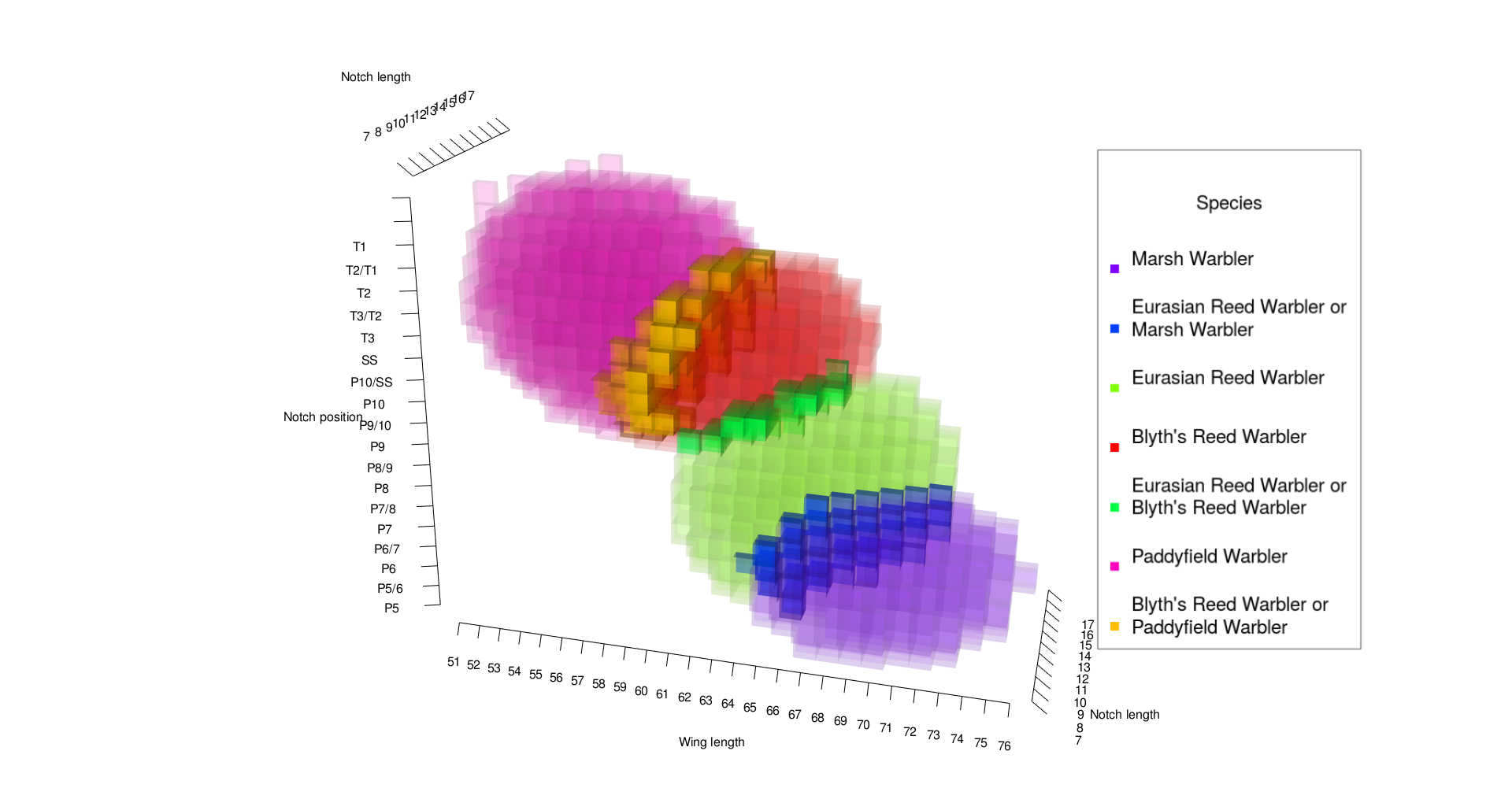
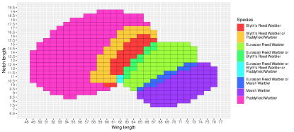
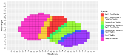
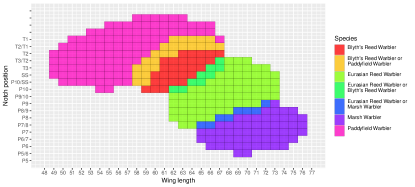
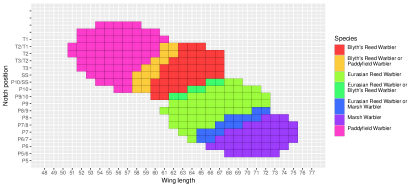
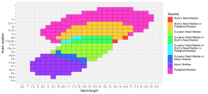
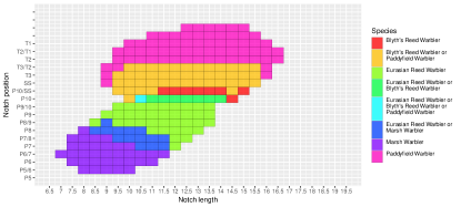
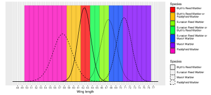
These probabilities are very close to the ones in Section 4.2, meaning we can hedge the risk of classifying something that might be a new species (not belonging to $\{1,\ldots,N\}$) entirely at a low cost. The decision regions for these values on $\rho$ and $\tau$ are presented graphically in Appendix E, where we cover all classification scenarios with missing trait values as well.

It is also possible to include classification with empty outputs in the context of indifference zones (Bechhofer, 1954; Goldsman, 1986). Assume that the parameter space is divided into $N+1$ regions, the first $N$ of which correspond to each of the $N$ hypotheses (or categories), whereas the last region of the parameter space (the indifference zone) corresponds to scenarios where no hypothesis is adequate. Based on this, it is possible to divide the test data space into $N+1$ regions as well, depending on whether the posterior distribution of the parameter puts most of its probability mass in any of the first $N$ parameter regions ($\hat{\mathrm{I}}=\{i\},i=1,\ldots,N$) or in the indifference zone ($\hat{\mathrm{I}}=\emptyset$).

4.4 Subproblem accessibility

Having fitted the model to the whole set of species, one may use the fit for any subproblem, e.g. classifying a bird between two species when the others are, for some reason, ruled out. Taking species 1 and 2, i.e. Eurasian Reed Warbler and Marsh Warbler, we estimate the probability of classifying wrongly and the probability of ending up in the indecisive region $\Lambda$ analogously with Section 4.2. Using $\rho=0.1$ and $\tau=0$, we find that

$$\begin{matrix}\hat{\mathbb{P}}\left(\mathrm{I}\notin\hat{\mathrm{I}}\mid x_{1}=0\right)=0.0037,&\hat{\mathbb{P}}\left(\mathrm{I}\notin\hat{\mathrm{I}}\mid x_{1}=1\right)=0.000971\end{matrix}$$

$$\begin{matrix}\hat{\mathbb{P}}\left(\lvert\hat{\mathrm{I}}\rvert>1\mid x_{1}=0\right)=0.0495,&\hat{\mathbb{P}}\left(\lvert\hat{\mathrm{I}}\rvert>1\mid x_{1}=1\right)=0.0099\end{matrix}$$

for this particular subproblem.

4.5 Choosing $\tau$

A potential risk for misclassification is observing a subject of a category not even considered for classification. In order to mitigate this, we introduced $\tau$ as a cut-off value for the trait distributions. Indeed, the value of $\tau$ determines how large deviations in trait measurements we accept without suspecting that we actually observe a subject from an unconsidered category. Choosing $\tau=0$ allows us to classify any point in the whole trait space, i.e. we believe the model is perfect in the sense that no unconsidered categories will be observed.

5 Model selection using cross-validation

Model selection can be used to select covariates and/or traits from a larger set by trading goodness-of-fit against parsimony for each candidate model $m$. Bayesian model selection requires a prior distribution on $m$ (Smith and Spiegelhalter, 1980; Kass and Raftery, 1995; Green, 1995; Tadesse et al., 2005). This approach involves the computationally intractable likelihood ${\cal L}({\cal D}_{i}^{obs})$ for each category $i$ and candidate model $m$. Non-Bayesian approaches, on the other hand, typically involve the observed likelihood ${\cal L}(\hat{\theta}_{i};{\cal D}_{i}^{obs})$ for each category $i$ and model $m$, with $\hat{\theta}_{i}$ the ML-estimator of $\theta_{i}$, as well as another term that penalizes large models. This includes the AIC (Akaike, 1974, 1998), NIC (Murata, 1991), BIC (Schwarz et al., 1978; Fraley and Raftery, 1998), and integrated complete-data likelihood (ICL; Biernacki et al., 2000) criteria, as well as stepwise model selection procedures based on pairwise hypothesis testing (McLachlan and Rathnayake, 2014). Here we will use an intermediate approach that retains the Bayesian assumption of random $\theta_{i}$ for each model $m$ but then compare these models in terms of their predictive performance. To this end we will use $\kappa$-fold cross validation. This will be illustrated on another original, unpublished data set, on two subspecies of Common chiffchaff (Phylloscopus collybita), the collybita and abietinus subspecies. It contains measurements for birds classified to subspecies visually by an expert at Falsterbo Bird Observatory.

5.1 Cross-validation for our type of models

The idea of $\kappa$-fold cross-validation is well established, and used for a very wide range of model families, see e.g. Wood (2017, p. 256). Choosing $\kappa=n_{i}$ for category $i$ corresponds to the basic form of cross-validation (Cover, 1969; Stone, 1974). This procedure is however computationally expensive, because one has to fit as many models ($=\sum_{i=1}^{N}n_{i}$) as there are observations. Since the method under study is already computationally intensive, in particular under widespread obfuscation, large $q$ and large data sets, we recommend using $\kappa$-fold cross-validation with $\kappa$ a bit smaller, i.e. a non-exhaustive cross-validation. In an interesting paper Kohavi (1995) examines cross-validation in general when choosing between classifiers. Kohavi concludes that $\kappa<n_{i}$ is generally preferred when picking the best classifier using cross-validation.

To perform $\kappa$-fold cross-validation in general for our class of models, we begin by choosing $\kappa\in\mathbb{Z}^{+}$ independently of $i$. Then create fold $l$ for category $i$ by choosing uniformly at random a set $J_{il}\subset\{1,\ldots,n_{i}\}$ comprising $n_{i}/\kappa$ or $n_{i}/\kappa+1$ observations of ${\cal D}^{\text{obs}}_{i}$, the training data at hand for category $i$. Repeat this for all categories until we have left-out test data sets $J_{l}=\cup_{i=1}^{N}J_{il}$ for $l=1,\ldots,\kappa$. Then for each $l$ proceed to fit models on the observations ${\cal D}^{\text{obs}}_{(-l)}={\cal D}^{\text{obs}}\setminus\{(x_{ij},\mathsf{S}_{ij});j\in J_{il}\}_{i=1}^{N}$ that were not left out and then estimate the posterior category probabilities $\hat{p}_{1}({\cal D}^{\text{obs}}_{(-l)},(x_{ij},\mathsf{S}_{ij})),\ldots,\hat{p}_{N}({\cal D}^{\text{obs}}_{(-l)},(x_{ij},\mathsf{S}_{ij}))$ for each observation $(x_{ij},\mathsf{S}_{ij})\in J_{l}$ that was left out. Choosing a reward function $R$, the corresponding classifier $\hat{\rm{I}}$ may be applied to each set of posterior probabilities in order to generate predictions $\hat{\mathrm{I}}_{(-l)ij}$ of the category, or set of categories, of the left-out observations contained in $J_{l}$. As this is repeated for each $l$, all observations will have been left out at one point when the cross validation is finished.

To assess the predictive performance of the $M$ models under consideration, let $w_{i}>0$ be weights such that $\sum_{i=1}^{N}w_{i}=1$, and compute

$$R^{\texttt{cv}}_{m}=\sum_{i=1}^{N}\frac{w_{i}}{n_{i}}\sum_{l=1}^{\kappa}\sum_{j\in J_{il}}R(\hat{\mathrm{I}}_{(-l)ij},i),$$ (23)

with a classifier (20) that corresponds to a prespecified value of $\rho$ and $\tau$, for $m=1,\ldots,M$, and an appropriately chosen reward function, such as (16) or (19). One could e.g. use the weights $w_{i}=n_{i}/\sum_{a=1}^{N}n_{a}$ or $w_{i}=1/N$, depending on whether it is more valuable to be able to predict a category with many observations or not. Based on (23), the best classifier is

$$\hat{m}=\operatorname*{arg\,max}_{m}\left(R^{\texttt{cv}}_{1},\ldots,R^{\texttt{cv}}_{M}\right).$$

When having computed $R^{\texttt{cv}}_{m}$, for $m=1,\ldots,M$, one has the possibility to choose a more parsimonious model that performes almost as well as $\hat{m}$, under the usual tradeoff between simplicity and predictive performance.

5.2 Choosing traits and covariates

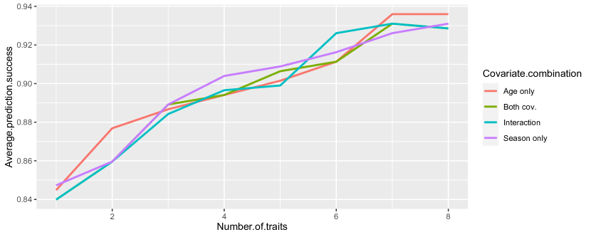
We will now examplify usage of cross validation with $\kappa=10$ folds for model selection. At hand we have a data set over two subspecies of Common chiffchaff (Phylloscopus collybita). Each subspecies has $q=9$ continuous traits measured. Although they are measured to half millimeters, we will regard them as perfect observations (${\cal D}^{\text{obs}}={\cal D}$), since the rounding bias is extremely small. Moreover we have two binary covariates (age and season), and we are interested in which combination of covariates and traits that best predicts the subspecies of a new bird. We will consider models with one covariate, both covariates and both covariates including an interaction term, meaning that the number of predictors $p$ ranges from 1 to 3.

For each covariate scenario, we fit a model $m$ with one trait, for each trait in turn, and then choose the one with the highest $R^{\texttt{cv}}$ value, based on the reward function (16). Keeping this trait, we then add another trait and repeat the procedure, and keep the two traits that yield the highest $R^{\texttt{cv}}$ value. The procedure is repeated until we have a model with 8 traits, and for each step, the value of $R^{\texttt{cv}}$ is stored. We used the weights $w_{i}=n_{i}/\sum_{k=1}^{N}n_{k}$ for all $i$, and put $\rho=1$ and $\tau=0$, i.e. used the classifier in (17) in the computation of $R^{\texttt{cv}}$.

The main reason for doing this forward selection-like procedure is to reduce the number of models that are fitted from about $(2^{9}-1)\cdot 4\cdot 10=20440$ (if every trait combination is tried) to $(9+8+\ldots+1)\cdot 4\cdot 10=1800$. Also, for each included trait, if the value of $R^{cv}$ does not increase, we may choose a more parsimonious model.

Figure 1 shows a plot of how $R^{\texttt{cv}}$ changes with the number of included traits for the various covariate combinations.

Figure 1: Each line represents, for a particular covariate combination, the change in average prediction success of the left-out data in the cross validation procedure, as the number of traits increases. In more detail, we use (16) as our reward function and $w_{i}=1/N$ for all categories $i$ in (23). No obvious differences between the covariate combinations are visible. It is, however, clear that 3 of the covariate scenarios reach their maximum cross-validation prediction accuracy with 7 traits. The set of included traits are not the same for all covariate scenarios.

5.3 Choosing $\rho$

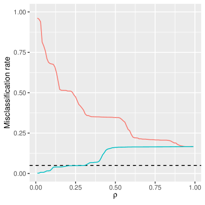
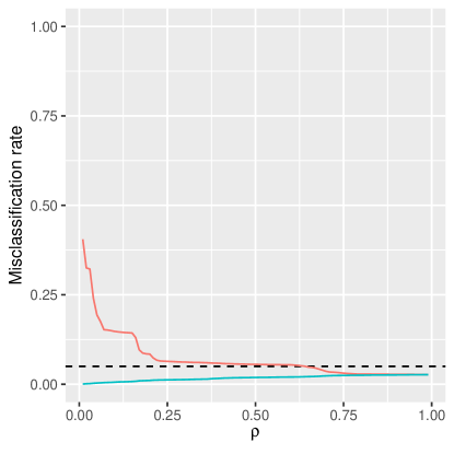
We will now present how the choice of $\rho$, for a classifier $\hat{I}$ based on a reward function (19), can be made more intuitive by letting the chosen value $\rho_{\delta}$ correspond to a highest acceptable misclassification rate $\delta$. To this end, we first introduce a reward function

$$\tilde{R}(\mathcal{I},i)=\begin{cases}1,\text{ if $i\in\mathcal{I}$,}\\ 0,\text{ otherwise,}\end{cases}$$ (24)

that outputs 1 when the true category belongs to the classified subset of categories, and otherwise 0. Interpreting $\tilde{R}(\mathcal{I},i)=1$ as a correct classification, we estimate the rate of correct classifications through cross-validation as

$$R_{\rho}^{\text{cv}}=\sum_{i=1}^{N}\frac{w_{i}}{n_{i}}\sum_{l=1}^{\kappa}\sum_{j\in J_{il}}\tilde{R}(\hat{\mathrm{I}}_{(-l)ij},i),$$ (25)

in analogy with (23). In order to speed up computation, we first perform cross-validation to generate category weights $\omega_{1}(x_{ij},\mathsf{S}_{ij}),\ldots,\omega_{N}(x_{ij},\mathsf{S}_{ij})$ for each observaton $(x_{ij},\mathsf{S}_{ij})$ in ${\cal D}^{\text{obs}}$. We then compute the probabilities $p_{1}(x_{ij},\mathsf{S}_{ij}),\ldots,$ $p_{N}(x_{ij},\mathsf{S}_{ij})$ of all categories according to (15), given a prior distribution $(\pi_{1},\ldots,$ $\pi_{N})$ on the categories. The category probabilities can then be used to create classifiers $\hat{I}_{(-l)ij}$ for each observation $(x_{ij},\mathsf{S}_{ij})$ with $j\in J_{l}$, for a grid of $\rho$-values. These classifiers are then inserted into (24), alongside the correct category, and the misclassification rate $1-R_{\rho}^{cv}$ is computed. We may then pick

$$\rho_{\delta}=\sup\{\rho^{\prime}:1-R_{\rho^{\prime}}^{\text{cv}}\leq\delta\}.$$ (26)

To illustrate this, we performed $\kappa=31$-fold cross-validation for the acrocephalus data. Recall that the majority of observations in these data are partial, and thus classification is hard (see e.g. the decision regions in Appendix E). To compute the category weights, for each fold $J_{l}$ we used the Bayes estimates $\hat{\theta}_{(-l)i}$ as in (7), based on the observations $(x_{ij},\mathsf{S}_{ij})$ of category $i$ not left out ($j\notin J_{l}$), as parameter values for the trait distributions. Then we numerically integrated

$$\omega_{\iota}(x_{ij},\mathsf{S}_{ij})=\int_{\mathsf{S}_{ij}}f\left(y;x_{ij},\hat{\theta}^{\text{(Bayes)}}_{(-l)\iota}\right)\,\mathrm{d}y,\quad\iota=1,\ldots,N,$$ (27)

for each $(x_{ij},\mathsf{S}_{ij})$ with $j\in J_{l}$ and $l=1,\ldots,\kappa$. We used two different priors in the computation of $p_{1}(x_{ij},\mathsf{S}_{ij}),\ldots,p_{N}(x_{ij},\mathsf{S}_{ij})$; a uniform prior ($\pi_{i}=1/N$ for all $i$) and a prior proportional to the number of observations in each category ($\pi_{i}=n_{i}/\sum_{\iota=1}^{N}n_{\iota}$). As in Section 5.2, we chose $w_{i}=n_{i}/\sum_{k=1}^{N}n_{k}$ for all $i$. The classifiers were created according to (20) and for $\rho=0.01,0.02,\ldots,0.99$ we computed (25) using two different reward functions. First the reward function $\tilde{R}(\mathcal{I},i)$, defined in (24), and then a second reward function

$$\dot{R}(\mathcal{I},i)=\begin{cases}1,\text{ if $i=\mathcal{I}$,}\\ 0,\text{ otherwise,}\end{cases}$$ (28)

which is more restrictive, as we consider the classifier to be correct when it contains only the correct category. The second reward function (28) is not used for choosing $\rho$, but rather in order to illustrate how its misclassification rate differs from the one obtained from the other less restrictive reward function $\tilde{R}$. The misclassification rates as functions of $\rho$ are presented in Figure 2 for both priors. In Table 4 we give the misclassification rates for each category using the uniform prior, for $\rho=1$ and $\rho=0.3$.

(a) Uniform prior.	(b) Proportional prior.

Figure 2: The graphs show the misclassification rate $1-R_{\rho}^{cv}$ as a function of $\rho$ for $\tilde{R}$ in blue and $\dot{R}$ in red. Notice how the two curves are both monotone in $\rho$ (but increasing and decreasing respectively) and converge at $\rho=1$, i.e. when both classifiers output sets of cardinality 1. The dashed black line is the chosen limit $\delta$ on the misclassification rate of 5%. For (a), the largest value of $\rho$ that does not exceed a misclassification rate of 5% (for reward function $\tilde{R}$) is $\rho_{0.05}=0.3$, at which 32.9% of the classified birds are wrong and/or contain two or more categories. For (b) the corresponding value of is $\rho_{0.05}=1$, and the misclassification rate is the same for both reward functions.

Species	$\rho=1$	$\rho=0.3$
Reed warbler	17.4%	5.1%
Blyth’s reed warbler	2.8%	0.9%
Paddyfield warbler	12.9%	3.2%
Marsh warbler	6.9%	2.2%

Table 4: The misclassification (as in rejecting the correct category) rate for each category using the uniform prior and reward function $\tilde{R}$. The majority of observations are partially observed leading to the high rates of misclassification (cf. Section 4).

The parameter $\rho$ can be used as a measure of how managable a classification problem is, given $\delta$. For any classification problem, we may first choose the misclassification rate upper limit $\delta$, and then find the highest value $\rho_{\delta}$ of $\rho$ for which the misclassification rate, based on reward function $\tilde{R}$, is below $\delta$. A more managable problem would then be one for which $\rho_{\delta}$ is higher. Classification problems where $\rho_{\delta}=1$ can be considered automizable, as there are sufficiently few dubious cases not to warrant any closer examination by an expert.

6 Comparison with discriminant analysis in the R package mclust

The mclust-package is the most popular package for multivariate clustering and classification (Scrucca et al., 2016) using R. It contains methods for clustering and classification of observations stemming from mixtures of Gaussian distributions, with cross-validation readily available to assess classification accuracy of the discriminant analysis models. We will use the discriminant analysis function MclustDA in order to compare its classification performance with our proposed method, using the Acrocephalus-data.

If one specifies prior distributions in the call to MclustDA, inference of model parameters is done through maximum aposteriori estimation (Fraley and Raftery, 2007). Then, in the next step these estimates are plugged into a Bayseian classifier with known parameters (Section 6.1 of Fraley and Raftery, 2002). In contrast, our classification scheme is fully Bayesian (14)-(15), with integration over posterior distributions of parameters. The priors on the model parameters differ somewhat, since we assume independent priors on the mean vector and covariance matrix of each class’ Gaussian distribution, whereas MclustDA does not (Fraley and Raftery, 2007). Moreover, we may specify priors for the mean vector for each class in our proposed method, while MclustDA does not permit this. Therefore, we chose the default option in MclustDA, which uses the mean of the traits from the data set. For our proposed method, we use the informative priors of Section 3.3. The prior on the species is uniform in the cross-validation scheme for both methods.

A further difference is that MclustDA do not permit the use of partial observations and covariates. Therefore, we reduce the Acrocephalus-data considerably to only consist of complete observations and partition it according to the binary covariate age. Consequently, two models are fitted with each method. These are then evaluated using 100-fold cross validation to estimate the prediction accuracy.

Results of the comparison of classification accuracy are presented in detail in Tables 5, 6 and 7. The take-away is that the methods preform similarily, except for juvenile birds, where our method to a larger extent than MclustDA classifies Reed warbler as Marsh warbler, and this is the source of its larger overall classification error probability among the juveniles.

Lastly, note also that the error probabilities with our method are higher than the estimated error probabilities (18) of Section 4.1. Although the estimates are computed in different ways, this nevertheless indicates the added value of including partial observations (as in Section 4.1) when available.

Table 5: Misclassification rate is the probability of classifying a new observation wrongly, estimated by 100-fold cross validation, when new observations are assumed to have a uniform distribution over species.

Misclassification rate	Method
Age class	mclust	K-H
Adult	3.05 %	3.56 %
Juvenile	1.59 %	3.74 %

Table 6: Classification table for adult birds using the cvMclustDA cross-validation method (referred to as mclust below), and the method proposed in this paper, (referred to as K-H below). The similarities of the methods are high, with a slightly higher accuracy for the mclust-method for Blyth’s reed warbler, and a slightly higher accuracy for the proposed method for the Paddyfield warbler.

	True species
	Reed warbler		Blyth’s reed w.		Paddyfield w.		Marsh warbler
Predicted species	mclust	K-H	mclust	K-H	mclust	K-H	mclust	K-H
Reed warbler	76	76	0	0	0	0	0	0
Blyth’s reed warbler	0	1	65	63	2	1	0	0
Paddyfield warbler	0	0	3	5	10	11	0	0
Marsh warbler	1	0	0	0	0	0	40	40

Table 7: Classification table for juveline birds using the cvMclustDA cross-validation method (referred to as mclust below), and the method proposed in this paper, (referred to as K-H below). The biggest difference between the two methods is in the lacking ability of K-H to classify Reed warblers correctly. As for adult birds, the proposed method has better accuracy for Paddyfield warblers, and contrary to adult birds, also for Blyth’s reed warbler, although the differences are small.

	True species
	Reed warbler		Blyth’s reed w.		Paddyfield w.		Marsh warbler
Predicted species	mclust	K-H	mclust	K-H	mclust	K-H	mclust	K-H
Reed warbler	403	382	0	0	0	0	5	5
Blyth’s reed warbler	0	2	40	41	2	1	0	0
Paddyfield warbler	0	0	1	0	16	17	0	0
Marsh warbler	6	25	0	0	0	0	409	409

7 Discussion

Throughout this paper, we have defined and analysed a classification problem with two sets of observations for each subject; its trait vector $Y$ and its covariate vector $x$, where $x$ is informative about the interpretation of $Y$. Since the trait values are often subject to various types of obfuscation, we set up a unified Bayesian framework for these situations, using a latent multivariate Gaussian distribution, with parameters estimated through supervised learning and a blockwise Gibbs sampling algorithm. To formalize the classification, we introduced reward functions with a set-valued input argument and two tuning parameters $\rho\in[0,1]$ and $\tau\in[0,1)$. The choice of $\rho$ affects the size and location of the indecisive region $\Lambda$ of our discriminant rule with a partial reject option. This region is the part of observational space where our classifer does not have sufficient information to rule out all but one category, whereas $\tau$ puts a limit on how much we allow an observation to deviate from the bulk of the data and still allowing it to be classified by our decision rule. Finally, we present a method of covariate and/or trait selection, through cross-validation, in order to obtain classifers that are both parsimonious and efficient.

Overall, there are two main usages of the method presented in this paper. First, one may derive distinguishing characteristics (cf. Appendix E) of the categories considered, due to interpretability. Secondly, one may use a fitted model to classify new observations with statistical rigour. An example of the usefulness of the first case would be an ornithologist with a set of birds of known taxa, who doesn’t know what morphologically separates these taxa. Using this method, she may extract for which trait measurements there is a high probability of certain taxa and thereby create (and write down) an identification key. Further, if there are too many combinations of trait levels to memorize, the Bayesian procedure we have described may perform the classification in an automized way.

A number of extensions of our work are possible. The first one regards the distribution of the latent variable. Although a Gaussian distribution is frequently used within quantitative genetics, there are instances when other distributions are preferable. As trait distribution, due to the central limit theorem, the Gaussian is particularly suitable when the traits are assumed to be polygenic and possibly affected by environmental factors (Lynch and Walsh, 1998). A conceptually critical but often numerically negligable adjustment is to correct all latent Gaussian distributions by truncating them to positive values for some of the traits. The trait wing length in our first real world example has to be positive by definition, and hence we should adjust our Gaussian distribution accordingly. However, considering the values of the parameter estimates (see Table 3), it would essentially make no difference to impose such a restriction for this particular data set. In other cases, it could be more important. When multimodality and skewness is a concern, an extension to hidden variables with a normal mixture distribution is an option (Hastie and Tibshirani, 1996; McParland et al., 2014).

A second extension is to incluce nominal (unordered) traits. This can be achieved by incorporating elements of a multinomial probit model (Geweke et al., 1994; McParland et al., 2014). Although bird traits are typically ordered, it might be of interest to incorporate nominal traits when more diverse taxa are classified, or when genetic data in terms of unordered genotypes is part of the trait vector.

Third, it would be of interest to consider model selection methods other than cross-validation. For instance, a Monte Carlo approximation of the BIC criterion, the so called BIC-MCMC approach, performed well in some previous analyses (Frühwirth-Schnatter, 2011; McParland et al., 2017).

Fourth, the reliance on training data with known categories can potentially be relaxed, or at least partially so. Without a reference material, which serves as training data, the nature of our problem would correspond to unsupervised learning and to a large extent fall under general model-based clustering (Fraley and Raftery, 2002; McParland et al., 2014, 2017) of observations taken from a mixture of multivariate Gaussian distributions. To take a step towards unsupervised learning in our setting, one would need to allow for indecisive regions where classification is ambigous. Such a clustering algorithm with partial reject options would transfer ideas in Chow (1970); Ripley (1996); Herbei and Wegkamp (2006) and this paper of having incomplete decisions, to a framework of unsupervised learning. A challenge in this context is to incorporate the effect of covariates. Specifying the number of clusters in advance would make the problem more well behaved, but might oftentimes be impossible, since the fundamental problem to solve in practice would be to determine this number of clusters. Still, this would allow the method to be used in situations where it is not known how to classify observations at all, and thus make it possible to investigate how many clusters a given data set supports.

Fifth, modifying the method slightly in order to handle repeated measurements is a straightforward task within our multivariate Gaussian framework. The benefit with repeated measurements of the traits is a better understanding of the magnitude of the measurement error, when trait vectors of observations are replaced by averaged trait vectors, for all repeated measurements. One could then include the number of measurements into the classification method, with direct effects on the size of the indecisive region and the accuracy of the classifier.

Sixth, as mentioned in Section 3, we assume prior independence between the regression parameters of different categories. This allows the effect of a covariate to vary between the categories, as opposed to forcing apriori a covariate to have the same effect across categories. However, Appendix D lists the posterior means of the covariate effects from our example model of Section 3.3, and one may notice that the effect is similar for some traits across categories, and to some extent even across traits. This indicates a general effect of our covariate, and hence we could construct a model that emphasizes such a general effect, by introducing apriori dependencies between the regression parameters of different species.

Finally, it is of interest to apply and extend our discrminant analysis method with partial reject options in order to analyze data sets where some observations are known to belong to several clusters (Latouche et al., 2011). This requires an extended type of reward function, $R(\mathcal{I},\mathrm{I})$, where both the classification $\mathcal{I}$ and the true $\mathrm{I}$ are sets of categories.

Appendix A Model formulation, complete data

Appendices A-E contain further mathematical details about the Bayesian model and classification procedure defined in Sections 3 and 4 respectively of the main article. In order to make the text self-contained, some details of the main article have been repeated. This Appendix A contains, in full detail, the derivation of estimators and the posterior category weights for a model using perfectly observed data. Posterior distributions for Bayesian multivariate linear regression with homoscedasticity assumption is readily available in Rossi et al. (2012, Sections 2.8 and 2.11), and we extend this to allow for heteroscedasticity.

Suppose we have $N$ different categories, contained in the set $\mathsf{N}=\{1,\ldots,N\}$, with prior probabilities $\pi=(\pi_{1},\ldots,\pi_{N})$. With full data we measure $q$ traits and $p$ covariates of each subject. Let $Y_{ijk}$ be the measurement of trait $k$ for subject $j$ in category $i$, where $1\leq i\leq N$, $1\leq j\leq n_{i}$, $1\leq k\leq q$ and $n_{i}$ is the number of subjects in category $i$. We assume that

$$Y_{ij}=(Y_{ij1},\ldots,Y_{ijq})\sim\text{N}\left(m_{ij},\mathbf{\Sigma}_{ij}\right)$$

are independent random vectors having a multivariate normal distribution, with

$$m_{ij}=(m_{ij1},\ldots,m_{ijq})\qquad\text{and}\qquad\mathbf{\Sigma}_{ij}=\left(\Sigma_{ijkl}\right)_{k,l=1}^{q}$$

being the mean vector and the covariance matrix of subject $j$ of category $i$. Let also

$$x_{ij}=\left(1,x_{ij1},\ldots,x_{ijp}\right)=\left(x_{ijm}\right)_{m=0}^{p}$$

be the covariate vector of subject $j$ of category $i$. Trait vectors and covariate vectors of category $i$ are rows in the matrices $\mathbf{Y}_{i}=\left(Y_{i1}^{\top},\ldots,Y_{in_{i}}^{\top}\right)^{\top}$ and $\mathbf{X}_{i}=\left(x_{i1}^{\top},\ldots,x_{in_{i}}^{\top}\right)^{\top}$ respectively. We now proceed by formulating a multivariate and multiple regression model

$$\mathbf{Y}_{i}=\mathbf{X}_{i}\mathbf{B}_{i}+\mathbf{E}_{i}$$ (29)

for category $i$, where $\mathbf{B}_{i}=\left(B_{imk};m=0,\ldots,p;k=1,\ldots,q\right)$ is the regression parameter matrix, whose first row consists of intercepts for the $q$ traits, $m_{ij}$ is the $j^{\text{th}}$ row of $\mathbf{X}_{i}\mathbf{B}_{i}$, and $\mathbf{E}_{i}=\left(E_{i1}^{\top},\ldots,E_{in_{i}}^{\top}\right)^{\top}$ is an error term matrix with independent rows $E_{ij}\sim\text{N}(0,\mathbf{\mathbf{\Sigma}}_{ij})$.

For use in the construction of a joint prior, and later the derivation of the marginal posterior distributions of the parameters, the vectorized form of our regression model is needed. Denote the operation of appending columns of a matrix by $\text{vec}(\cdot)$ (we will also use the inverse operation $\text{vec}^{-1}(\cdot)$ on column vectors) and rewrite (29) as

$$\mathbf{U}_{i}=\text{vec}(\mathbf{Y}_{i})=\mathbf{Z}_{i}\beta_{i}+\text{vec}(\mathbf{E}_{i})$$ (30)

with $\beta_{i}=\text{vec}(\mathbf{B}_{i})$. Denoting an identity matrix of rank $q$ with $\mathbf{I}_{q}$ and using the matrix tensor product $\otimes$,

$$\mathbf{Z}_{i}=\mathbf{I}_{q}\otimes\mathbf{X}_{i}=\begin{pmatrix}\mathbf{X}_{i}&0&\cdots&0\\ 0&\mathbf{X}_{i}&\ddots&\vdots\\ \vdots&\ddots&\ddots&0\\ 0&\cdots&0&\mathbf{X}_{i}\end{pmatrix}$$ (31)

is a block-diagonal matrix with $q$ blocks along the diagonal.

Now suppose we have $A$ covariance classes $\alpha=1,\ldots,A$ for category $i$ such that

$$\mathbf{\Sigma}_{ij}=\mathbf{\Sigma}^{\alpha}_{i}\quad\text{if }x_{ij}\in\mathcal{X}^{\alpha},$$ (32)

where $\mathcal{X}=\mathcal{X}^{1}\cup\ldots\cup\mathcal{X}^{A}$ is a disjoint decomposition of the predictor space $\mathcal{X}$. Assuming a prior $\text{N}\left(\left(b_{i0k},\ldots,b_{ipk}\right)^{\top}=b_{ik},\mathbf{\Sigma}_{\mathbf{B}_{i}}\right)$ on each of the columns $k=1,\ldots,q$ of $\mathbf{B}_{i}$, we obtain a prior $\text{N}\left(\left(b_{i1}^{\top},\ldots,b_{iq}^{\top}\right)^{\top}=\beta_{i0},\mathbf{I}_{q}\otimes\mathbf{\Sigma}_{\mathbf{B}_{i}}=\mathbf{\Sigma}_{\beta_{i}}\right)$ on $\beta_{i}$. Further, assuming prior independence of $\beta_{i},\mathbf{\Sigma}_{i}^{1},\ldots,\mathbf{\Sigma}_{i}^{A}$ and imposing an Inverse-Wishart distribution $\mathbf{\Sigma}_{i}^{\alpha}\sim IW(\nu_{0},\mathbf{V}_{0})$ on the covariance matrices in (32) for $\alpha=1,\ldots,A$, we get the joint prior

$$p(\beta_{i},\mathbf{\Sigma}_{i}^{1},\ldots,\mathbf{\Sigma}_{i}^{A})=p(\beta_{i})\prod_{\alpha=1}^{A}p(\mathbf{\Sigma}_{i}^{\alpha})$$ (33)

for the parameters of category $i$.

A.1 Estimation

Let $\theta_{i}=\left(\mathbf{B}_{i},\mathbf{\Sigma}^{1}_{i},\ldots,\mathbf{\Sigma}_{i}^{A}\right)$ represent all parameters of category $i$. In the following, we assume that $\theta_{1},\ldots,\theta_{N}$ are independent random vectors with probability densities $p(\theta_{1}),\ldots,p(\theta_{N})$ defined in (33). Introducing dependencies is of course possible, and may be important for specific problems. This is briefly mentioned in Section 7 of the main paper. From Bayes’ Theorem we get an aposteriori density

$$p(\theta_{i}\mid{\cal D}_{i}) =p(\theta_{i}){\cal L}\left({\cal D}_{i}\right)^{-1}\prod_{j=1}^{n_{i}}f\left(y_{ij};x_{ij},\theta_{i}\right)$$

$$=p(\theta_{i}){\cal L}\left({\cal D}_{i}\right)^{-1}{\cal L}(\theta_{i};{\cal D}_{i})$$

$$\propto p(\theta_{i}){\cal L}(\theta_{i};{\cal D}_{i})$$

of $\theta_{i}$ given the complete training data set ${\cal D}_{i}=\{(x_{ij},Y_{ij});\,j=1,\ldots,n_{i}\}=\{\mathbf{X}_{i},\mathbf{Y}_{i}\}$ for category $i$. The function ${\cal L}\left(\theta_{i};{\cal D}_{i}\right)=p\left(\mathbf{Y}_{i}\mid\mathbf{X}_{i},\theta_{i}\right)$ is the likelihood, whereas ${\cal L}({\cal D}_{i})=p({\cal D}_{i})$ is the marginal likelihood of category $i$. In the last step we removed the normalizing factor ${\cal L}({\cal D}_{i})^{-1}$, since it does not depend on $\theta_{i}$. The Maximum Aposteriori (MAP)-estimator of $\theta_{i}$ is

$$\theta^{(\text{MAP})}_{i} =\operatorname*{arg\,max}_{\theta_{i}}p(\theta_{i}\mid{\cal D}_{i})$$

$$=\operatorname*{arg\,max}_{\theta_{i}}p(\theta_{i}){\cal L}(\theta_{i};{\cal D}_{i}),$$

whereas the Bayes’ estimator of $\theta_{i}$ is

$$\theta^{(\text{Bayes})}_{i} =\mathbb{E}\left[\theta_{i}\mid{\cal D}_{i}\right]$$

$$=\int\!\theta_{i}p(\theta_{i}\mid{\cal D}_{i})\,\mathrm{d}\theta_{i}$$

$$={\cal L}\left({\cal D}_{i}\right)^{-1}\int\!\theta_{i}p(\theta_{i}){\cal L}(\theta_{i};{\cal D}_{i})\,\mathrm{d}\theta_{i}.$$

Finally, given a new observation ${\cal D}^{\text{new}}=(x,Y)$, define the posterior probability of the new observation belonging to category $i$ as

$$p_{i}=\mathbb{P}(\mathrm{I}=i\mid{\cal D},{\cal D}^{\text{new}})=\frac{\pi_{i}\omega_{i}}{\pi_{1}\omega_{1}+\ldots+\pi_{N}\omega_{N}},$$ (34)

where

$$\omega_{i} =\int\!f(Y;x,\theta_{i})p(\theta_{i}\mid{\cal D}_{i})\,\mathrm{d}\theta_{i}$$

$$={\cal L}({\cal D}_{i})^{-1}\int\!f(Y;x,\theta_{i})p(\theta_{i})\mathcal{L}(\theta_{i};{\cal D}_{i})\,\mathrm{d}\theta_{i}$$

are the posterior category weights given ${\cal D}^{\text{new}}$ for all categories, before the prior probabilities $\pi_{i}$ have been taken into account.

A.2 Monte Carlo Approximations

It is usually difficult to evaluate the normalizing constants ${\cal L}({\cal D}_{i})^{-1}$ for high-dimensional data sets, and hence also $\theta^{(\text{Bayes})}_{i}$ and $\omega_{i}$. However, it is possible to estimate $\theta^{(\text{Bayes})}_{i}$ and $\omega_{i}$ by Monte Carlo simulation, with

$$\hat{\theta}^{\text{(Bayes)}}_{i}=\frac{1}{R_{i}}\sum_{r=1}^{R_{i}}\theta_{ir}$$ (35)

and

$$\hat{\omega}_{i}=\frac{1}{R_{i}}\sum_{r=1}^{R_{i}}f(Y;x,\theta_{ir})$$ (36)

respectively, if $\theta_{i1},\ldots,\theta_{iR_{i}}$ are $R_{i}$ replicates drawn from the posterior distribution $p(\theta_{i}\mid{\cal D}_{i})$, with $\theta_{ir}=\left(\beta_{ir},\mathbf{\Sigma}_{ir}^{1},\ldots,\mathbf{\Sigma}_{ir}^{A}\right)$.

We will generate $\theta_{i1},\ldots,\theta_{iR_{i}}$ by blockwise Gibbs sampling, and for this we need the conditional posterior distributions of $\beta_{i}$ and $\mathbf{\Sigma}_{i}^{\alpha}$ for $\alpha=1,\ldots,A$. To derive those, we need some additional notation. Let $\mathbf{Z}_{i}^{\alpha}$, $\mathbf{X}_{i}^{\alpha}$, $\mathbf{Y}_{i}^{\alpha}$ and $\mathbf{U}_{i}^{\alpha}$ denote the submatrices of $\mathbf{Z}_{i}$, $\mathbf{X}_{i}$, $\mathbf{Y}_{i}$ and $\mathbf{U}_{i}$ corresponding to covariance class $\alpha$, and let $\mathbf{I}_{n}$ be the identity matrix of order $n$. Recall also that $\mathbf{B}_{i}=\text{vec}^{-1}(\beta_{i})$, meaning that we know $\mathbf{B}_{i}$ from $\beta_{i}$, and vice versa. For simplicity of notation we omit index $i$ in the following proposition:

Proposition 1.

Denote the parameter vector of a Bayesian multivariate multiple regression model with $A$ covariance classes by $\theta=\left(\beta,\mathbf{\Sigma}^{1},\ldots,\mathbf{\Sigma}^{A}\right)$, where $\beta$ is the regression parameter vector and $\mathbf{\Sigma}^{1},\ldots,\mathbf{\Sigma}^{A}$ are the $A$ covariance matrices. Let the prior of $\theta$ be $p(\theta)=p(\beta)\prod_{\alpha=1}^{A}p(\mathbf{\Sigma}^{\alpha})$, where $\beta\sim\text{N}(\beta_{0},\mathbf{\Sigma}_{\beta})$ and $\mathbf{\Sigma}^{\alpha}\sim IW(\nu_{0},\mathbf{V}_{0})$ for $\alpha=1,\ldots,A$. Then the posterior distribution of $\beta\mid\mathbf{U},\mathbf{Z},\mathbf{\Sigma}^{1},\ldots,\mathbf{\Sigma}^{\alpha}$ is $\text{N}(\tilde{\beta},\tilde{\mathbf{\Sigma}})$, where

$$\tilde{\mathbf{\Sigma}} =\left[\mathbf{\Sigma}_{\beta}^{-1}+\sum_{\alpha=1}^{A}(\mathbf{\Sigma}^{\alpha})^{-1}\otimes\left(\mathbf{X}^{\alpha}\right)^{\top}\mathbf{X}^{\alpha}\right]^{-1}$$

and

$$\tilde{\beta} =\tilde{\mathbf{\Sigma}}\times\left[\mathbf{\Sigma}_{\beta}^{-1}\beta_{0}+\sum_{\alpha=1}^{A}\left(\left(\mathbf{\Sigma}^{\alpha}\right)^{-1}\otimes\left(\mathbf{X}^{\alpha}\right)^{\top}\right)\mathbf{U}^{\alpha}\right].$$

Proof.

By applying Bayes’ theorem

$$p\left(\beta\mid\mathbf{U},\mathbf{Z},\mathbf{\Sigma}^{1},\ldots\mathbf{\Sigma}^{A}\right) \propto\exp\left\{-\frac{1}{2}(\beta-\beta_{0})^{\top}\mathbf{\Sigma}_{\beta}^{-1}(\beta-\beta_{0})\right\}\cdot$$

$$\cdot\prod_{\alpha=1}^{A}\exp\left\{-\frac{1}{2}\left(\mathbf{U}^{\alpha}-\mathbf{Z}^{\alpha}\beta\right)^{\top}\left(\mathbf{\Sigma}^{\alpha}\otimes\mathbf{I}_{n^{\alpha}}\right)^{-1}\left(\mathbf{U}^{\alpha}-\mathbf{Z}^{\alpha}\beta\right)\right\}$$

$$=\exp\left\{-\frac{1}{2}\beta\mathbf{C}\beta+\beta\mathbf{D}\right\}$$

where $n^{\alpha}$ is the number of observations in covariance class $\alpha$,

$$\mathbf{C} =\mathbf{\Sigma}_{\beta}^{-1}+\sum_{\alpha=1}^{A}(\mathbf{Z}^{\alpha})^{\top}(\mathbf{\Sigma}^{\alpha}\otimes\mathbf{I}_{n^{\alpha}})^{-1}\mathbf{Z}^{\alpha}$$

$$=\mathbf{\Sigma}_{\beta}^{-1}+\sum_{\alpha=1}^{A}\left(\mathbf{Z}^{\alpha}(\mathbf{\Sigma}^{\alpha}\otimes\mathbf{I}_{p+1})^{-1}\right)^{\top}\mathbf{Z}^{\alpha}$$

$$=\mathbf{\Sigma}_{\beta}^{-1}+\sum_{\alpha=1}^{A}((\mathbf{\Sigma}^{\alpha})^{-1}\otimes\mathbf{I}_{p+1})(\mathbf{Z}^{\alpha})^{\top}\mathbf{Z}^{\alpha}$$

$$=\mathbf{\Sigma}_{\beta}^{-1}+\sum_{\alpha=1}^{A}\left(\mathbf{\Sigma}^{\alpha}\right)^{-1}\otimes\left(\mathbf{X}^{\alpha}\right)^{\top}\mathbf{X}^{\alpha},$$

where in the second step of the last equation we used Lemma 1 below, and

$$\mathbf{D} =\mathbf{\Sigma}_{\beta}^{-1}\beta_{0}+\sum_{\alpha=1}^{A}(\mathbf{Z}^{\alpha})^{\top}(\mathbf{\Sigma}^{\alpha}\otimes\mathbf{I}_{n^{\alpha}})^{-1}\mathbf{U}^{\alpha}$$

$$=\mathbf{\Sigma}_{\beta}^{-1}\beta_{0}+\sum_{\alpha=1}^{A}\left(\left(\mathbf{\Sigma}^{\alpha}\right)^{-1}\otimes\left(\mathbf{X}^{\alpha}\right)^{\top}\right)\mathbf{U}^{\alpha}.$$

Consequently,

$$\beta\mid\mathbf{U},\mathbf{Z},\mathbf{\Sigma}^{1},\ldots,\mathbf{\Sigma}^{A}\sim N(\tilde{\beta},\tilde{\mathbf{\Sigma}})$$

where

$$\tilde{\beta} =\mathbf{C}^{-1}\mathbf{D}$$

$$=\left[\mathbf{\Sigma}_{\beta}^{-1}+\sum_{\alpha=1}^{A}(\mathbf{\Sigma}^{\alpha})^{-1}\otimes\left(\mathbf{X}^{\alpha}\right)^{\top}\mathbf{X}^{\alpha}\right]^{-1}$$

$$\times\left[\mathbf{\Sigma}_{\beta}^{-1}\beta_{0}+\sum_{\alpha=1}^{A}\left(\left(\mathbf{\Sigma}^{\alpha}\right)^{-1}\otimes\left(\mathbf{X}^{\alpha}\right)^{\top}\right)\mathbf{U}^{\alpha}\right]$$

and

$$\tilde{\mathbf{\Sigma}}=\mathbf{C}^{-1}=\left[\mathbf{\Sigma}_{\beta}^{-1}+\sum_{\alpha=1}^{A}(\mathbf{\Sigma}^{\alpha})^{-1}\otimes\left(\mathbf{X}^{\alpha}\right)^{\top}\mathbf{X}^{\alpha}\right]^{-1}.$$

Notice that $\tilde{\beta}$ is a multivariate version of a weighted average of the prior vector $\beta_{0}$ and the least squares estimates of $\beta$ obtained from the $A$ covariance classes. ∎

The following lemma was used in the proof of Proposition 1. It admits a considerable gain in computational speed, when calculating the posterior covariance matrix $\tilde{\mathbf{\Sigma}}$.

Lemma 1.

Let $\mathbf{Z}$ be a block-diagonal $nq\times(p+1)q$ matrix, where there are $q$ blocks $\mathbf{X}$, which are $n\times(p+1)$-matrices, along the diagonal. Let $\mathbf{\Sigma}$ be a symmetric, positive definite $q\times q$-matrix. Then it holds that

$$\mathbf{Z}^{\top}\left(\mathbf{\Sigma}\otimes\mathbf{I}_{n}\right)^{-1}\mathbf{Z}=\left(\mathbf{Z}\left(\mathbf{\Sigma}\otimes\mathbf{I}_{p+1}\right)^{-1}\right)^{\top}\mathbf{Z}.$$

Proof.

We prove the lemma by iterated use of the mixed-product property of the tensor product. Since $\mathbf{Z}=\left(\mathbf{I}_{q}\otimes\mathbf{X}\right)$, the left hand side becomes

$$\left(\mathbf{I}_{q}\otimes\mathbf{X}\right)^{\top}\left(\mathbf{\Sigma}\otimes\mathbf{I}_{n}\right)^{-1}\left(\mathbf{I}_{q}\otimes\mathbf{X}\right) =\left(\mathbf{I}_{q}\otimes\mathbf{X}^{\top}\right)\left(\mathbf{\Sigma}^{-1}\otimes\mathbf{I}_{n}\right)\left(\mathbf{I}_{q}\otimes\mathbf{X}\right)$$

$$=\left(\mathbf{I}_{q}\mathbf{\Sigma}^{-1}\otimes\mathbf{X}^{\top}\mathbf{I}_{n}\right)\left(\mathbf{I}_{q}\otimes\mathbf{X}\right)$$

$$=\left(\mathbf{\Sigma}^{-1}\otimes\mathbf{X}^{\top}\right)\left(\mathbf{I}_{q}\otimes\mathbf{X}\right)$$

$$=\mathbf{\Sigma}^{-1}\mathbf{I}_{q}\otimes\mathbf{X}^{\top}\mathbf{X}$$

$$=\mathbf{\Sigma}^{-1}\otimes\mathbf{X}^{\top}\mathbf{X}$$

and the right hand side becomes

$$\left(\left(\mathbf{I}_{q}\otimes\mathbf{X}\right)\left(\mathbf{\Sigma}\otimes\mathbf{I}_{p+1}\right)^{-1}\right)^{\top}\left(\mathbf{I}_{q}\otimes\mathbf{X}\right) =\left(\mathbf{I}_{q}\mathbf{\Sigma}^{-1}\otimes\mathbf{X}\mathbf{I}_{p+1}\right)^{\top}\left(\mathbf{I}_{q}\otimes\mathbf{X}\right)$$

$$=\left(\mathbf{\Sigma}^{-1}\otimes\mathbf{X}\right)^{\top}\left(\mathbf{I}_{q}\otimes\mathbf{X}\right)$$

$$\{\text{by symmetry of $\mathbf{\Sigma}$}\} =\left(\mathbf{\Sigma}^{-1}\otimes\mathbf{X}^{\top}\right)\left(\mathbf{I}_{q}\otimes\mathbf{X}\right)$$

$$=\mathbf{\Sigma}^{-1}\mathbf{I}_{q}\otimes\mathbf{X}^{\top}\mathbf{X}$$

$$=\mathbf{\Sigma}^{-1}\otimes\mathbf{X}^{\top}\mathbf{X}$$

which proves the lemma already in the third equalities. ∎

Using the vector form, we may express the conditional posterior of the regression parameters

$$\beta_{i}\mid\mathbf{U}_{i},\left\{\mathbf{\Sigma}_{i}^{\alpha}\right\}_{\alpha=1}^{A}\sim\text{N}(\tilde{\beta},\tilde{\mathbf{\Sigma}})$$

where

$$\tilde{\mathbf{\Sigma}}=\left[\mathbf{\Sigma}_{\beta}^{-1}+\sum_{\alpha=1}^{A}\left(\mathbf{\Sigma}_{i}^{\alpha}\right)^{-1}\otimes\left(\left(\mathbf{X}_{i}^{\alpha}\right)^{\top}\mathbf{X}_{i}^{\alpha}\right)\right]^{-1},$$

and

$$\tilde{\beta} =\tilde{\mathbf{\Sigma}}\times\left[\mathbf{\Sigma}_{\beta}^{-1}\beta_{0}+\sum_{\alpha=1}^{A}\left(\left(\mathbf{\Sigma}_{i}^{\alpha}\right)^{-1}\otimes\left(\mathbf{X}_{i}^{\alpha}\right)^{\top}\right)\mathbf{U}_{i}^{\alpha}\right].$$

Meanwhile, the conditional posteriors of the covariance matrices are

$$\mathbf{\Sigma}_{i}^{\alpha}\mid\mathbf{B}_{i},\mathbf{Y}_{i}^{\alpha},\mathbf{X}_{i}^{\alpha} \sim IW(\nu_{0}+n_{i}^{\alpha},\mathbf{V}_{0}+\mathbf{S}^{\alpha}_{i}),$$

where $n_{i}^{\alpha}$ denotes the number of observations in the covariance class $\alpha$ for category $i$ and

$$\mathbf{S}_{i}^{\alpha}=\left(\mathbf{Y}_{i}^{\alpha}-\mathbf{X}_{i}^{\alpha}\mathbf{B}_{i}\right)^{\top}\left(\mathbf{Y}_{i}^{\alpha}-\mathbf{X}_{i}^{\alpha}\mathbf{B}_{i}\right)$$

Having computed $\hat{\omega}_{1},\ldots,\hat{\omega}_{N}$, for ${\cal D}^{\text{new}}$, we may compute the Monte Carlo-estimated aposteriori probability of ${\cal D}^{\text{new}}$ being in category $i$ as

$$\hat{p}_{i}=\hat{\mathbb{P}}(I=i\mid{\cal D},{\cal D}^{\text{new}})=\frac{\pi_{i}\hat{\omega}_{i}}{\pi_{1}\hat{\omega}_{1}+\ldots+\pi_{N}\hat{\omega}_{N}},$$

where ${\cal D}={\cal D}_{1}\cup\ldots\cup{\cal D}_{N}$ is the complete training data set.

Appendix B Model Formulation, obfuscated data

Overall our setup is the same as in Appendix A, but we now suppose there is only partial information about the complete training data set ${\cal D}$. Due to some obfuscation, which could be due to rounding, grouping, categorization or lost measurements of some traits, we only know that

$$Y_{ij}\in\mathsf{S}_{ij}=\mathsf{S}_{ij1}\times\cdots\times\mathsf{S}_{ijq},$$

i.e. the complete trait vector $Y_{ij}$ for subject $j$ of category $i$ is contained in a hyperrectangle $\mathsf{S}_{ij}$, whose components are given by $\{\mathsf{S}_{ijk}\}_{k=1}^{q}$. The components are sets, ranging in possible size from singletons to infinite intervals of $\mathbb{R}$, and are given by

$$\mathsf{S}_{ijk}=\begin{cases}Y_{ijk},&k\notin\mathsf{K}_{ij},\\ \left(c_{ijk},d_{ijk}\right],&k\in\mathsf{K}_{ij},\end{cases}$$

where $\mathsf{K}_{ij}=\left\{k;1\leq k\leq q;\,Y_{ijk}\text{ obfuscated}\right\}$. As described in the main article, without loss of generality we assume that $z_{ijk}$, the mid point of $(c_{ijk},d_{ijk}]$ for finite sets, is integer-valued.

We can treat all types of obfuscations uniformly in the following way. Suppose trait $k$ of subject $j$ of category $i$ is imperfectly observed, i.e. $k\in\mathsf{K}_{ij}$. Let $g_{k}$ be the number of categories of this trait, which we number as $0,1,\ldots,g_{k}-1$. The observed category is $z_{ijk}\in\left\{0,1,\ldots,g_{k}-1\right\}$, where $g_{k}=2$ for binary data and $g_{k}=\infty$ for count data. The corresponding side of $\mathsf{S}_{ij}$ is

$$\mathsf{S}_{ijk}=\begin{cases}\left(-\infty,\frac{1}{2}\right],&\text{if }z_{ijk}=0,\\ \left(z_{ijk}-\frac{1}{2},z_{ijk}+\frac{1}{2}\right],&\text{if }1\leq z_{ijk}\leq g_{k}-2,\\ \left(g_{k}-\frac{3}{2},\infty\right),&\text{if }z_{ijk}=g_{k}-1.\end{cases}$$

We also write

$$Z_{ijk}=z(\mathsf{S}_{ijk})=\begin{cases}0,&\text{if }\mathsf{S}_{ijk}=\left(-\infty,\frac{1}{2}\right],\\ \frac{c_{ijk}+d_{ijk}}{2},&\text{if $\mathsf{S}_{ijk}$ is bounded},\\ g_{k}-1,&\text{if }\mathsf{S}_{ijk}=\left(g_{k}-\frac{3}{2},\infty\right],\end{cases}$$

for the center point of a finite or half-open, infinite $\mathsf{S}_{ijk}$, whereas $z\left(\mathsf{S}_{ijk}\right)=Y_{ijk}$ when $Y_{ijk}=\mathsf{S}_{ijk}$ is perfectly observed. We may write the actually observed training data set as

$${\cal D}^{\text{obs}}=\left\{\left(x_{ij},\mathsf{S}_{ij}\right);\,i=1,\ldots,N,j=1,\ldots,n_{i}\right\}.$$

B.1 Estimation

Using ${\cal D}^{\text{obs}}_{i}=\{(x_{ij},\mathsf{S}_{ij});j=1,\ldots,n_{i}\}$, the posterior distribution of $\theta_{i}$ becomes

$$p(\theta_{i}\mid{\cal D}^{\text{obs}}_{i}) =p(\theta_{i}){\cal L}\left({\cal D}^{\text{obs}}_{i}\right)^{-1}\prod_{j=1}^{n_{i}}p(\mathsf{S}_{ij};x_{ij},\theta_{i})$$

$$=p(\theta_{i}){\cal L}\left({\cal D}^{\text{obs}}_{i}\right)^{-1}{\cal L}(\theta_{i};{\cal D}^{\text{obs}}_{i}),$$ (37)

where the normalizing factor

$${\cal L}\left({\cal D}^{\text{obs}}_{i}\right)=\int\!p(\theta_{i}){\cal L}(\theta_{i};{\cal D}^{\text{obs}}_{i})\,\mathrm{d}\theta_{i}$$

is the marginal likelihood of category $i$, and

$$p(\mathsf{S}_{ij},x_{ij};\theta_{i})=\begin{cases}f(Y_{ij};x_{ij},\theta_{i}),&\mathsf{K}_{ij}=\emptyset,\\ \int_{\mathsf{S}_{ij}}\!f(y_{ij};x_{ij},\theta_{i})\prod_{k\in\mathsf{K}_{ij}}\mathrm{d}y_{ijk},&\mathsf{K}_{ij}\neq\emptyset.\end{cases}$$ (38)

Thus, with perfect observations ($\mathsf{K}_{ij}=\emptyset$), we evaluate the density of the trait vector $f$ at the observed point $Y_{ij}$ and the model is exactly as specified in Appendix A. Otherwise, we construct a $\left|\mathsf{K}_{ij}\right|$-dimensional integral over $f$ and the contribution to the likelihood is this integral, with the function evaluated exactly at the remaining perfectly observed traits, if any exist. In particular, if all traits are imperfectly observed, the integral is $q$-dimensional. We may approximate the integral in (38) by

$$\left|\mathsf{S}_{ij}\right|f\left(z(\mathsf{S}_{ij}),x_{ij};\theta_{i}\right)=\prod_{k\in\mathsf{K}_{ij}}\left|\mathsf{S}_{ijk}\right|\cdot f\left(z(\mathsf{S}_{ij1}),\ldots,z(\mathsf{S}_{ijq}),x_{ij};\theta_{i}\right)$$

whenever all $\left|\mathsf{S}_{ijk}\right|<\infty$ for $k\in\mathsf{K}_{ij}$, which is the case when employing the trick with auxiliary categories, mentioned in Section 3.2 of the main article.

Alternatively, since $p(\mathsf{S}_{ij},x_{ij};\theta_{i})$ potentially contains integrals of a multivariate Gaussian density function and there in general is a lack of a CDF on closed form for this distribution, the integrals in (38) need to be solved numerically. However, in the case of $|\mathsf{K}_{ij}|=1$, with $\mathsf{K}_{ij}=\{k\}$ and $\mathsf{S}_{ijk}=\left(c_{ijk},d_{ijk}\right]$, the integral is univariate and thus

$$p(\mathsf{S}_{ij},x_{ij};\theta_{i}) =f(Y_{ij(-k)},x_{ij};\theta_{i})\bigg{[}\Phi\left(\frac{d_{ijk}-m_{ijk}(y_{ij(-k)})}{\sigma_{ijk}}\right)$$ (39)

$$-\Phi\left(\frac{c_{ijk}-m_{ijk}(y_{ij(-k)})}{\sigma_{ijk}}\right)\bigg{]},$$

where $m_{ijk}(y_{ij(-k)})=m_{ijk}+\mathbf{\Sigma}_{ijk(-k)}\mathbf{\Sigma}_{ij(-k)(-k)}^{-1}(y_{ij(-k)}-m_{ij(-k)})$ is the conditional expectation of $Y_{ijk}$ given that $Y_{ij(-k)}=(Y_{ijk^{\prime}};\,k^{\prime}\neq k)=y_{ij(-k)}$, $\sigma_{ijk}=\sqrt{\mathbf{\Sigma}_{ijkk}-\mathbf{\Sigma}_{ijk(-k)}\mathbf{\Sigma}_{ij(-k)(-k)}^{-1}\mathbf{\Sigma}_{ij(-k)k}}$ is the conditional standard deviation of $Y_{ijk}$ given any value of $Y_{ij(-k)}$, and $\Phi$ is the CDF of the univariate Gaussian distribution with mean 0 and standard deviation 1.

Using ${\cal D}^{\text{obs}}_{i}$, we find from (B.1) that the estimators $\theta^{(\text{MAP})}_{i}$ and $\theta^{(\text{Bayes})}_{i}$ are

$$\theta^{(\text{MAP})}_{i} =\operatorname*{arg\,max}_{\theta_{i}}p(\theta_{i}\mid{\cal D}^{\text{obs}}_{i})$$

$$=\operatorname*{arg\,max}_{\theta_{i}}p(\theta_{i}){\cal L}({\cal D}^{\text{obs}}_{i};\theta_{i})$$

and

$$\theta^{(\text{Bayes})}_{i} =\mathbb{E}\left[\theta_{i}\mid{\cal D}^{\text{obs}}_{i}\right]=\int\!\theta_{i}p(\theta_{i}\mid{\cal D}^{\text{obs}}_{i})\,\mathrm{d}\theta_{i}$$

$$={\cal L}\left({\cal D}^{\text{obs}}_{i}\right)^{-1}\int\!\theta_{i}p(\theta_{i}){\cal L}({\cal D}^{\text{obs}}_{i};\theta_{i})\,\mathrm{d}\theta_{i}$$ (40)

respectively. Furthermore, redefining ${\cal D}^{\text{new}}:=(x,\mathsf{S})$ for a new observation, where $\mathsf{S}=\mathsf{S}_{1}\times\ldots\times\mathsf{S}_{q}$, and denoting the corresponding set of imperfectly observed traits by $\mathsf{K}$, leads to the posterior category weights

$$\omega_{i} =\iint_{\mathsf{S}}\!f(y;x,\theta_{i})\prod_{k\in\mathsf{K}}\mathrm{d}y_{k}\,p(\theta_{i}\mid{\cal D}^{\text{obs}}_{i})\,\mathrm{d}\theta_{i}$$

$$={\cal L}\left({\cal D}^{\text{obs}}_{i}\right)^{-1}\iint_{\mathsf{S}}\!f(y;x,\theta_{i})\prod_{k\in\mathsf{K}}\mathrm{d}y_{k}\,p(\theta_{i}){\cal L}({\cal D}^{\text{obs}}_{i};\theta_{i})\,\mathrm{d}\theta_{i}$$ (41)

of this observation.

B.2 Monte Carlo Approximations

The integral over $\mathsf{S}$ in (41) is, as mentioned in conjunction with (39), potentially impossible to compute analytically, but could also be well behaved. We can in theory approximate $\theta^{(\text{Bayes})}_{i}$ in (B.1) as in (35) by sampling $\theta_{i}$ from $p(\theta_{i}\mid{\cal D}^{\text{obs}})$ a total of $R_{i}$ times. However, this entails a large number of numerical evaluations of integrals, see (B.1)-(38). Similarly, we may estimate $\omega_{i}$ for $1\leq i\leq N$ in (41) through

$$\hat{\omega}_{i}=\frac{1}{R_{i}}\sum_{r=1}^{R_{i}}\int_{\mathsf{S}}f(y;x,\theta_{ir})\prod_{k\in\mathsf{K}}\mathrm{d}y_{k},$$ (42)

which in addition to previously presented integrals, involves computation of an integral over $\mathsf{S}$. As an alternative way of computing (B.1) and (42), we also present an approach where complete data is sampled, based on the obfuscated data, as one step of the Monte Carlo algorithm, whereas the parameters are sampled as another step of the same algorithm. This allows us to estimate all $\theta^{(\text{Bayes})}_{i}$ and $\omega_{i}$ under widespread obfuscation, given that we are able to simulate $\mathbf{Y}_{i}$, $i=1,\ldots,N$. Overall, we want to generate

$$\left\{\theta_{ir},Y_{ijkr},\,1\leq j\leq n_{i},\,k\in\mathsf{K}_{ij};Y_{kr},k\in\mathsf{K}\right\}_{r=1}^{R_{i}}$$ (43)

from

$$p(\theta_{i}|{\cal D}^{\text{obs}}_{i})\prod_{j=1}^{n_{i}}f\left(y_{ij\mathsf{K}_{ij}r}\mid x_{ij},\mathsf{S}_{ij},\theta_{i}\right)f\left(y_{\mathsf{K}r},\mid x,Y_{\mathsf{K}^{\complement}};\theta_{i}\right)$$ (44)

where $\theta_{ir}=\left(\beta_{ir},\mathbf{\Sigma}_{ir}^{1},\ldots,\mathbf{\Sigma}_{ir}^{A}\right)$, $y_{ij\mathsf{K}_{ij}r}=\left(y_{ijkr};k\in\mathsf{K}_{ij}\right)$, $y_{\mathsf{K}r}=\left(y_{kr};k\in\mathsf{K}\right)$ and $Y_{\mathsf{K}^{\complement}}=\left(Y_{k};k\notin\mathsf{K}\right)$. Note that we do not condition on $\mathsf{S}$ in the conditional density of the unobserved traits for the new observation that we want to classify, as this would introduce a bias in the Monte Carlo estimate of $\omega_{i}$ below.

The details of the specific Gibbs sampling approach we use are presented in Appendix C. Having generated a sample $\theta_{i1},\ldots,\theta_{iR_{i}}$, we may compute the estimated category weights of ${\cal D}^{\text{new}}$ as

$$\hat{\omega}_{i}=\frac{1}{R_{i}}\sum_{r=1}^{R_{i}}f\left(Y_{\mathsf{K}^{\complement}};x,\theta_{ir}\right)\mathbbm{1}_{\left\{Y_{\mathsf{K}r}\in\bigtimes_{k\in\mathsf{K}}\mathsf{S}_{k}\right\}},$$ (45)

where $Y_{\mathsf{K}^{\complement}}$ is as above, and $Y_{\mathsf{K}r}=\left(Y_{kr};k\in\mathsf{K}\right)$. For every $\theta_{ir}$, one could generate many $Y_{\mathsf{K}}$ and replace the indicator with an average of the indicators for each sampled $Y_{\mathsf{K}}$.

A potentially more efficient method would be to define $\{y_{t}\}_{t=1}^{T}$, where $y_{t}=(y_{t1},\ldots,y_{tq})$ with $y_{t\mathsf{K}^{\complement}}=Y_{\mathsf{K}^{\complement}}$ and $y_{t\mathsf{K}}\in\bigtimes_{k\in\mathsf{K}}\mathsf{S}_{k}$, in such a way that $\{y_{tk},k\in\mathsf{K}\}$ is a grid approximation of $\bigtimes_{k\in\mathsf{K}}\mathsf{S}_{k}$. Then we can estimate $\omega_{i}$ through

$$\hat{\omega}_{i}=\frac{\prod_{k\in\mathsf{K}}\lvert\mathsf{S}_{k}\rvert}{TR_{i}}\sum_{r=1}^{R_{i}}\sum_{t=1}^{T}f\left(y_{t};x,\theta_{ir}\right).$$ (46)

If we use the trick with auxiliary categories described in Section 3.2 of the main article, we can we can choose $y_{t}$ uniformly at random on $\bigtimes_{k\in\mathsf{K}}\mathsf{S}_{k}$, as long as we do not have any missing observations, since those are represented with an infinite interval. Thus, (46) is potentially more effcient than (45), but comes at a cost of generality, since (45) is applicable to any new observation.

Finally, the Monte Carlo-estimated aposteriori probability of ${\cal D}^{\text{new}}=(x,\mathsf{S})$ being of category $i$ is

$$\hat{p}_{i}=\hat{\mathbb{P}}(I=i\mid{\cal D}^{\text{new}},{\cal D}^{\text{obs}})=\frac{\pi_{i}\hat{\omega}_{i}}{\pi_{1}\hat{\omega}_{1}+\ldots+\pi_{N}\hat{\omega}_{N}}$$ (47)

and we may apply (41) with replacement of $\omega_{i}$ by (45) for prediction. If (46) is inserted into (47) we notice that $\prod_{k\in\mathsf{K}}\lvert\mathsf{S}_{k}\rvert$ and $T$ cancel out, and in case $R_{i}=R$ for $i=1,\ldots,N$, also $R$ cancels out.

Appendix C Gibbs sampling details

The focus of this appendix is Procedure 1, in which we describe in detail how to generate a sample of size $R_{i}$ from the posterior distribution of the parameter vector $\theta_{i}$, using blockwise Gibbs sampling. It describes the general case, i.e. when we have obfuscated trait measurements in ${\cal D}^{\text{obs}}$. For the case with perfectly observed trait measurements, we skip the sampling of $\mathbf{Y}_{i}$ and use the observed values instead, otherwise the procedure is the same. Applying the procedure to data from each category $i$ will yield all the samples we need from the posterior distribution in order to perform classification.

In Procedure 1, $TN(\mu,\mathbf{\Sigma},\mathsf{S})$ refers to the truncated Gaussian distribution, where $\mu$ is the mean vector, $\mathbf{\Sigma}$ is the covariance matrix and $\mathsf{S}$ is a hyper rectangle specifying the truncation limits. Simulating from this distribution can be done exactly using rejection sampling, or approximately using an inner Gibbs algorithm. Depending on application, either approach can be preferred, as the tradeoff is exact sampling versus efficiency. Also, more advanced algorithms such as Importance Sampling-techniques can be used in this step.

Procedure 1 The Monte Carlo approach to sampling the parameters’ posterior distribution under obfuscation.

0:  ${\cal D}^{\text{obs}},\nu_{0},\mathbf{V}_{0},\beta_{i0}=\text{vec}(\mathbf{B}_{i0})$

0:  A sample of size $R_{i}$ from the posterior distribution of $\theta_{i}$.

  for $\alpha=1\to A$ do

     draw $\mathbf{\Sigma}_{i0}^{\alpha}\sim IW\left(\nu_{0},\mathbf{V}_{0}\right)$

  end for

  draw $\beta_{i0}\sim\text{N}\left(\beta_{i0},\mathbf{\Sigma}_{\beta_{i}}\right)$

  $\theta_{i0}\leftarrow\left(\beta_{i0},\mathbf{\Sigma}_{i0}^{1},\ldots,\mathbf{\Sigma}_{i0}^{A}\right)$

  for $r=1\to R_{i}$ do

     for $j=1\to n_{i}$ do

        draw $\mathbf{Y}_{ij,r-1}\mid x_{ij},\mathsf{S}_{ij},\theta_{i,r-1}\sim TN\left(\mathbf{X}_{ij}\mathbf{B}_{i,r-1},\mathbf{\Sigma}_{ij,r-1},\mathsf{S}_{ij}\right)$

     end for

     $\mathbf{U}_{i,r-1}\leftarrow\text{vec}(\mathbf{Y}_{i,r-1})$

     draw $\beta_{ir}\mid\mathbf{U}_{i(r-1)},\left\{\mathbf{\Sigma}_{i(r-1)}^{\alpha}\right\}_{\alpha=1}^{A}\sim\text{N}\left(\tilde{\beta},\tilde{\mathbf{\Sigma}}\right)$

     for $\alpha=1\to A$ do

        draw $\mathbf{\Sigma}_{ir}^{\alpha}\mid\mathbf{U}_{i(r-1)}^{\alpha},\mathbf{X}_{i}^{\alpha},\beta_{ir}\sim IW(\nu_{0}+n_{i}^{\alpha},\mathbf{V}_{0}+\mathbf{S}_{i}^{\alpha})$

     end for

     $\theta_{ir}\leftarrow\left(\beta_{ir},\mathbf{\Sigma}_{ir}^{1},\ldots,\mathbf{\Sigma}_{ir}^{A}\right)$

     save $\theta_{ir}$

  end for

Appendix D Highest posterior density intervals of parameters

Table 8: Quantiles of the posterior distribution for the parameters of the Acrocephalus model. The values in the ad-columns are the change in intercept for adult birds in the Regression parameter values-section, and separate values in the other sections. We have chosen to present the correlation between traits instead of the covariances. Notice the very slim posterior density intervals for Reed Warbler and Marsh Warbler, since we have lots of observations for these species, and the widely dispersed posterior distributions for Paddyfield Warbler, being a species with very few observations and a vague prior on the covariance matrices.

	Regression parameter values						Variance estimates						Correlation estimates
	Wing		Notch		Notch pos.		Wing		Notch		Notch pos.		Wing-N.		Wing-N.p.		N. - N.p.
Quantile	juv	ad	juv	ad	juv	ad	juv	ad	juv	ad	juv	ad	juv	ad	juv	ad	juv	ad
Reed warbler 2.5%	66.69	0.7	10.99	1.27	107.87	1.95	2.31	2.61	0.57	0.55	1.28	1.3	0.46	0.33	-0.09	0.00	0.46	0.29
50%	66.7	0.73	11.07	1.38	108	2.29	2.35	2.67	0.63	0.62	1.48	1.59	0.52	0.41	0.02	0.20	0.54	0.45
97.5%	66.72	0.76	11.13	1.52	108.13	2.56	2.38	2.74	0.71	0.72	1.66	2.35	0.57	0.49	0.13	0.37	0.61	0.60
Marsh warbler 2.5%	69.99	0.57	9.42	0.54	104.86	0.39	2.07	2.28	0.41	0.47	0.69	0.5	0.37	0.36	-0.13	-0.12	0.23	0.03
50%	70.05	0.69	9.45	0.61	104.96	0.66	2.19	2.51	0.44	0.53	0.8	0.76	0.40	0.43	-0.03	0.16	0.33	0.28
97.5%	70.1	0.81	9.48	0.68	105.04	1	2.32	2.76	0.47	0.6	0.92	1.16	0.44	0.49	0.06	0.41	0.42	0.49
Paddyfield warbler 2.5%	56.64	-0.74	12.24	0.4	114.8	0.05	1.28	2.36	0.49	0.76	0.77	0.68	-0.20	-0.08	-0.58	-0.11	-0.13	-0.03
50%	57.27	0.36	12.66	1.16	115.32	0.81	2.17	4.32	0.83	1.35	1.3	1.24	0.19	0.37	-0.25	0.35	0.27	0.42
97.5%	57.89	1.47	13.1	1.89	115.83	1.61	4	9.07	1.52	2.77	2.46	2.6	0.53	0.69	0.15	0.68	0.59	0.72
Blyth’s reed warbler 2.5%	61.84	-0.48	12.23	0.8	113.23	0.63	1.31	1.34	0.47	0.61	0.6	0.87	0.07	0.29	-0.18	-0.17	-0.09	0.09
50%	62.26	0.03	12.49	1.13	113.53	1.03	1.94	1.85	0.69	0.83	0.9	1.2	0.35	0.49	0.12	0.07	0.21	0.32
97.5%	62.69	0.56	12.75	1.46	113.85	1.43	3.04	2.64	1.08	1.17	1.37	1.71	0.58	0.64	0.40	0.30	0.47	0.51

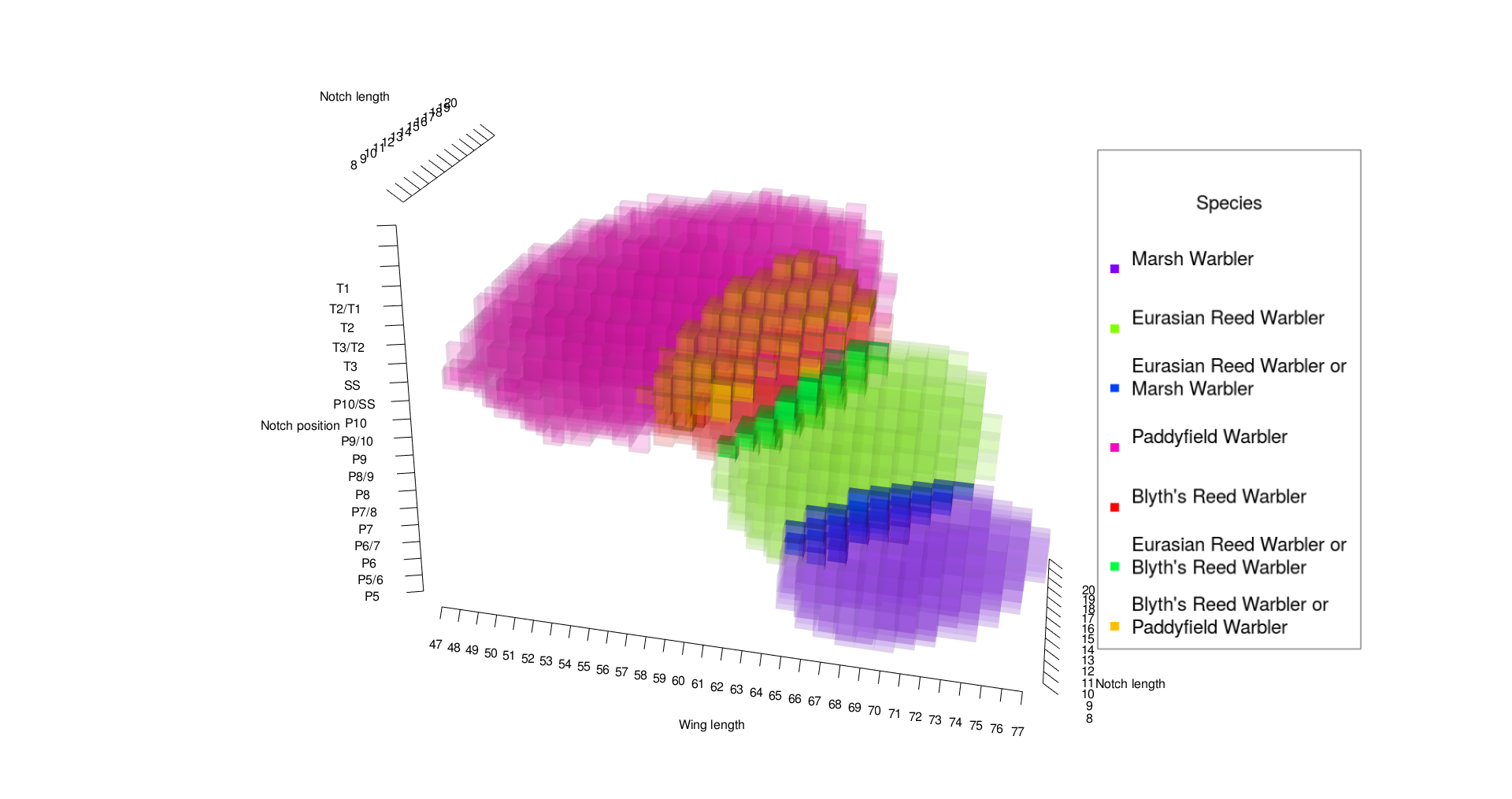
Appendix E Visualized decision regions

All of these visualizations are done using the same model fit and the same generated new observations from the posterior predictive distribution as in Section 4 of the main text. As a reminder, we used the values $\rho=0.1$ and $\tau=0.001$ for the tuning parameters of the classifier.

(a) Adult birds.	(b) Juvenile birds.

Figure 3: Decision regions when observing all three traits of the Acrocephalus warblers. Completely transparent blocks represent observations that will be classified as outliers, i.e. not get any species assigned to them. The indecisive region $\Lambda$ is less transparent, and colored according to which species there are uncertainty about. The probability of observing an individual that belongs to the indecisive region is $0.0820$ for (a) and $0.0791$ for (b), when each species is equally likely apriori to occur. The decision region of Paddyfield Warbler partially engulfs Blyth’s Reed Warbler for adult birds, reflecting the large uncertainty in the parameter estimates for adult Paddyfield Warblers. Notice also that we introduce unnamed categories for notch position, as the predictive posterior distribution requires this.

(a) Adult birds.	(b) Juvenile birds.

Figure 4: Decision regions when only observing wing and notch length.

(a) Adult birds.	(b) Juvenile birds.

Figure 5: Decision regions when only observing wing length and notch position.

(a) Adult birds.	(b) Juvenile birds.

Figure 6: Decision regions when only observing notch length and notch position.

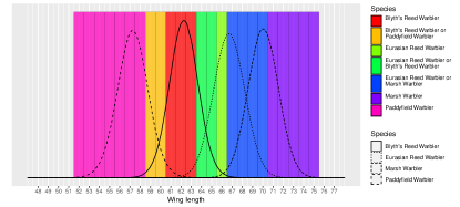(a) Adult birds.	(b) Juvenile birds.

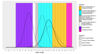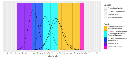(c) Adult birds.	(d) Juvenile birds.

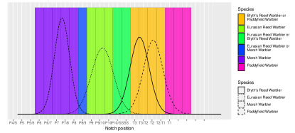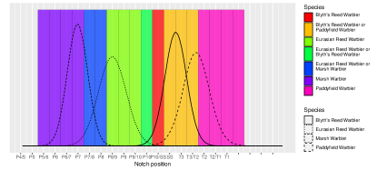(e) Adult birds.	(f) Juvenile birds.

Figure 7: In (a) and (b), decision regions are shown when only wing length is observed; in (c) and (d) decision regions are shown when only notch length is observed; and in (e) and (f) decision regions are shown when only notch position is observed. In all plots, kernel density estimates of each aposteriori trait distribution for each species is shown with black lines of different types. The plot highlights the larger degree of separation in the traits wing length and notch position.

References

- Aitchison and Dunsmore (1980) Aitchison, J. and I. R. Dunsmore (1980). Statistical prediction analysis. CUP Archive.
- Akaike (1974) Akaike, H. (1974). A new look at the statistical model identification. IEEE Transactions on Automatic Control 19(6), 716–723.
- Akaike (1998) Akaike, H. (1998). Information theory and an extension of the maximum likelihood principle. In Selected papers of hirotugu akaike, pp. 199–213. Springer.
- Albert and Chib (1993) Albert, J. H. and S. Chib (1993). Bayesian Analysis of Binary and Polychotomos Response Data. Journal of the American Statistical Association 88(422), 669–679.
- Barnett et al. (1979) Barnett, J. A., R. W. Payne, and D. Yarrow (1979). A guide to identifying and classifying yests. Cambridge University Press.
- Bechhofer (1954) Bechhofer, R. E. (1954). A single-sample multiple decision procedure for ranking means of normal populations with known variances. The Annals of Mathematical Statistics, 16–39.
- Bensmail and Celeux (1996) Bensmail, H. and G. Celeux (1996). Regularized gaussian discriminant analysis through eigenvalue decomposition. Journal of the American statistical Association 91(436), 1743–1748.
- Biernacki et al. (2000) Biernacki, C., G. Celeux, and G. Govaert (2000). Assessing a mixture model for clustering with the integrated completed likelihood. IEEE transactions on pattern analysis and machine intelligence 22(7), 719–725.
- Bouveyron and Brunet (2012) Bouveyron, C. and C. Brunet (2012). Probabilistic fisher disrciminant analysis: A robust and flexible alternative to fisher discriminant analysis. Neurocomputing 90, 12–22.
- Carlin et al. (1998) Carlin, B. P., J. B. Kadane, and A. E. Gelfand (1998). Approaches for optimal sequential decision analysis in clinical trials. Biometrics, 964–975.
- Chow (1970) Chow, C. (1970). On optimum recognition error and reject tradeoff. IEEE Transactions on information theory 16(1), 41–46.
- Chu and Ghahramani (2005) Chu, W. and Z. Ghahramani (2005). Gaussian processes for ordinal regression. Journal of Machine Learning Research 6, 1019–1041.
- Cortes and Vapnik (1995) Cortes, C. and V. Vapnik (1995). Support vector networks. Machine Learning 20, 273–279.
- Cover (1969) Cover, T. M. (1969). Learning in pattern recognition. In Methodologies of pattern recognition, pp. 111–132. Elsevier.
- De Leon and Chough (2013) De Leon, A. R. and K. C. Chough (2013). Analysis of mixed data: methods & applications. CRC Press.
- DeGroot (1970) DeGroot, M. H. (1970). Optimal statistical decisions. McGraw-Hill, New York.
- Domingos and Pazzani (1997) Domingos, P. and M. Pazzani (1997). On the optimality of the simple bayesian classifier under zero-one loss. Machine Learning 29, 103–130.
- D’Orazio (2021) D’Orazio, M. (2021). Distances with mixed type variables, some modified gower’s coefficients. arXiv 2101.02481.
- Felsenstein (1983) Felsenstein, J. (Ed.) (1983). Numerical taxonomy. Springer Verlag, Berlin.
- Fisher (1936) Fisher, R. (1936). The use of multiple measurements in taxonomic problems. Annals of Eugenics 7, 179–188.
- Fokoué and Titterington (2003) Fokoué, E. and D. Titterington (2003). Mixtures of factor analysers. bayesian estimation and inference by stochastic simulation. Machine Learning 50(1), 73–94.
- Fox (2010) Fox, J.-P. (2010). Bayesian item response modeling: Theory and applications. Springer Science & Business Media.
- Fraley and Raftery (1998) Fraley, C. and A. E. Raftery (1998). How many clusters? which clustering method? answers via model-based cluster analysis. The computer journal 41(8), 578–588.
- Fraley and Raftery (2002) Fraley, C. and A. E. Raftery (2002). Model-based clustering, discriminant analysis, and density estimation. Journal of the American statistical Association 97(458), 611–631.
- Fraley and Raftery (2007) Fraley, C. and A. E. Raftery (2007). Bayesian regularization for normal mixture estimation and model-based clustering. Journal of classification 24(2), 155–181.
- Freund et al. (2004) Freund, Y., Y. Mansour, R. E. Schapire, et al. (2004). Generalization bounds for averaged classifiers. Annals of Statistics 32(4), 1698–1722.
- Friedman (1989) Friedman, J. (1989). Regularized discriminant analysis. Journal of the American Statistical Association 84, 165–175.
- Friedman et al. (2000) Friedman, J., J. Hastie, and R. Tibshirani (2000). Additive logistic regression: A statistical view of boosting. Annals of Statistics 28, 337–407.
- Frühwirth-Schnatter (2011) Frühwirth-Schnatter, S. (2011). Label switching under model uncertainty. Mixtures: Estimation and Application, 213–239.
- Gao et al. (2017) Gao, X., H. Lin, K. Revanna, and Q. Dong (2017). Naive bayesian classifier for rapid assignment of rrna sequences into new bacterial taxonomy. BMC Bioinformatics 18(247).
- Geisser (1964) Geisser, S. (1964). Posterior odds for multivariate normal classifications. Journal of the Royal Statistical Society: Series B (Methodological) 26(1), 69–76.
- Geisser (1993) Geisser, S. (1993). Predictive inference, Volume 55. CRC press.
- Gelman et al. (2013) Gelman, A., J. B. Carlin, H. S. Stern, D. B. Dunson, A. Vehtari, and D. B. Rubin (2013). Bayesian data analysis. CRC press.
- Geman and Geman (1984) Geman, S. and D. Geman (1984). Stochastic relaxation, gibbs distributions, and the bayesian restoration of images. IEEE Transactions on pattern analysis and machine intelligence (6), 721–741.
- Geweke et al. (1994) Geweke, J., M. Keane, and D. Runkle (1994). Alternative computational approaches to inference in the multinomial probit model. The review of economics and statistics, 609–632.
- Goldsman (1986) Goldsman, D. (1986). Tutorial on indifference-zone normal means ranking and selection procedures. In Proceedings of the 18th conference on Winter simulation, pp. 370–375.
- Gower (1971) Gower, J. (1971). A general coefficient of similarity and some of its properties. Biometrics 27, 623–637.
- Gower and Legendre (1986) Gower, J. and P. Legendre (1986). Metric and euclidean properties of dissimilarithy coefficients. Journal of Classification 3, 5–48.
- Green (1995) Green, P. (1995). Reversible jump mcmc computation and bayesian model determination. biomeirika, 82: 711-732 hastings, wk 1970. monte carlo sampling methods using markov chains and their applications. Biometrika 57, 97–109.
- Hastie and Tibshirani (1996) Hastie, T. and R. Tibshirani (1996). Discriminant analysis by gaussian mixture. Journal of the Royal Statistical Socierty B 58(1), 155–176.
- Hastie et al. (2009) Hastie, T., R. Tibshirani, and J. Friedman (2009). The elements of statistical learning: Data mining, inference, and prediction. (2 ed.). Springer-Verlag, New York.
- Herbei and Wegkamp (2006) Herbei, R. and M. H. Wegkamp (2006). Classification with reject option. The Canadian Journal of Statistics/La Revue Canadienne de Statistique, 709–721.
- Hjort (1986) Hjort, N. L. (1986). Notes on the Theory of Statistical Symbol Recognition: Automatic Segmentation and Symbol Recognition of Linelike Drawings [ASSEL]. Norsk Regnesentral.
- Huelsenbeck and Ronquist (2001) Huelsenbeck, J. and F. Ronquist (2001). Mrbayes: Bayesian inference of phylogenetic trees. Bioinformatics 17(8), 754–755.
- Kass and Raftery (1995) Kass, R. E. and A. E. Raftery (1995). Bayes factors. Journal of the american statistical association 90(430), 773–795.
- Kauffmann and Rousseeuw (1990) Kauffmann, L. and P. J. Rousseeuw (1990). Finding Groups in Data: An Introduction to Cluster Analysis. Wiley Series in Probability and Statistics.
- Kohavi (1995) Kohavi, R. (1995). A study of cross-validation and bootstrap for accuracy estimation and model selection. In International Joint Conference on Artificial Intelligence, Volume 14, pp. 1137–1145. Montreal, Canada.
- Kumar and Andreou (1998) Kumar, N. and A. Andreou (1998). Heteroscedastic discriminant analysis and reduced rank hmms for improved speech recognition. Speech Communications 26(4), 283–297.
- Lande et al. (2003) Lande, R., S. Engen, B.-E. Saether, et al. (2003). Stochastic population dynamics in ecology and conservation. Oxford University Press on Demand.
- Latouche et al. (2011) Latouche, P., E. Birmelé, C. Ambroise, et al. (2011). Overlapping stochastic block models with application to the french political blogosphere. The Annals of Applied Statistics 5(1), 309–336.
- LeCun et al. (1989) LeCun, Y., B. Boser, J. S. Denker, D. Henderson, R. E. Howard, W. Hubbard, and L. D. Jackel (1989). Backpropagation applied to handwritten zip code recognition. Neural computation 1(4), 541–551.
- Lin et al. (2000) Lin, X., G. Wahba, D. Xiang, F. Gao, R. Klein, and B. Klein (2000). Smoothing spline anova models for large data sets with bernoulli obsevations and the randomized gacv. Annals of Statistics 28, 1570–1600.
- Liu et al. (2011) Liu, Y., H. H. Zhang, and Y. Wu (2011). Hard of soft classification? large-margin unified machines. Journal of the American Statistical Association 106(493), 166–177.
- Lord (1952) Lord, F. M. (1952). The relation of the reliability of multiple-choice tests to the distribution of item difficulties. Psychometrika 17(2), 181–194.
- Lord and Novick (2008) Lord, F. M. and M. R. Novick (2008). Statistical theories of mental test scores. IAP.
- Lynch and Walsh (1998) Lynch, M. and B. Walsh (1998). Genetics and analysis of quantitative traits. Sinauer Associates, Sunderland MA.
- Macedo and Oliveira (2013) Macedo, H. D. and J. N. Oliveira (2013). Typing linear algebra: A biproduct-oriented approach. Science of Computer Programming 78(11), 2160–2191.
- Malmhagen et al. (2013) Malmhagen, B., M. Karlsson, and S. Menzie (2013). Using wing morphology to separate four species of Acrocephalus warblers in Scandinavia. Ringing & Migration 28(1), 63–68.
- Marron et al. (2007) Marron, J., M. J. Todd, and J. Ahn (2007). Distance-weighted discrimination. Journal of the Amererican Statistical Association 102(480), 1267–1271.
- McLachlan and Rathnayake (2014) McLachlan, G. J. and S. Rathnayake (2014). On the number of components in a gaussian mixture model. Wiley Interdisciplinary Reviews: Data Mining and Knowledge Discovery 4(5), 341–355.
- McParland et al. (2014) McParland, D., I. C. Gormley, T. H. McCormick, S. J. Clark, C. W. Kabudula, and M. A. Collinson (2014). Clustering south african households based on their asset status using latent variable models. The annals of applied statistics 8(2), 747.
- McParland et al. (2017) McParland, D., C. M. Phillips, L. Brennan, H. M. Roche, and I. C. Gormley (2017). Clustering high-dimensional mixed data to uncover sub-phenotypes: joint analysis of phenotypic and genotypic data. Statistics in medicine 36(28), 4548–4569.
- Murata (1991) Murata, N. (1991). A criterion for determining the number of parameters in an artificial neural network model. Artificial Neural Networks 1, 9–14.
- Payne and Preece (1980) Payne, R. and D. Preece (1980). Identification keys and diagnostic tables: A review. Journal of the Royal Statistical Society A 143(3), 253–292.
- R Core Team (2021) R Core Team (2021). R: A Language and Environment for Statistical Computing. Vienna, Austria: R Foundation for Statistical Computing.
- Rasch (1993) Rasch, G. (1993). Probabilistic models for some intelligence and attainment tests. ERIC.
- Ripley (1996) Ripley, B. D. (1996, January). Pattern recognition and neural networks. Cambridge university press.
- Robert and Casella (2013) Robert, C. and G. Casella (2013). Monte Carlo statistical methods. Springer Science & Business Media.
- Rossi et al. (2012) Rossi, P. E., G. M. Allenby, and R. McCulloch (2012). Bayesian statistics and marketing. John Wiley & Sons.
- Schwarz et al. (1978) Schwarz, G. et al. (1978). Estimating the dimension of a model. Annals of statistics 6(2), 461–464.
- Scrucca et al. (2016) Scrucca, L., M. Fop, T. B. Murphy, and A. E. Raftery (2016). mclust 5: clustering, classification and density estimation using Gaussian finite mixture models. The R Journal 8(1), 289–317.
- Smith and Spiegelhalter (1980) Smith, A. F. and D. J. Spiegelhalter (1980). Bayes factors and choice criteria for linear models. Journal of the Royal Statistical Society: Series B (Methodological) 42(2), 213–220.
- Smith (1946) Smith, C. A. (1946). Some examples of discrimination. Annals of Eugenics 13(1), 272–282.
- Sneath and Sokal (1973) Sneath, P. H. and R. R. Sokal (1973). Numerical Taxonomy. The principles and practice of numerical classification. Freeman, San Francisco.
- Spearman (1904) Spearman, C. (1904). ”general intelligence”, objectively determined and measured. The American Journal of Psychology 15, 201–293.
- Stone (1974) Stone, M. (1974). Cross-validatory choice and assessment of statistical predictions. Journal of the Royal Statistical Society: Series B (Methodological) 36(2), 111–133.
- Svensson (1992) Svensson, L. (1992). Identification guide to European passerines. L. Svensson.
- Tadesse et al. (2005) Tadesse, M. G., N. Sha, and M. Vannucci (2005). Bayesian variable selection in clustering high-dimensional data. Journal of the American Statistical Association 100(470), 602–617.
- Thurstone (1925) Thurstone, L. L. (1925). A method of scaling psychological and educational tests. Journal of educational psychology 16(7), 433.
- Tricker (1984) Tricker, A. (1984). Effects of rounding on the moments of a probability distribution. Journal of the Royal Statistical Society: Series D (The Statistician) 33(4), 381–390.
- Vermunt (2001) Vermunt, J. K. (2001). The use of restricted latent class models for defining and testing nonparametric and parametric item response theory models. Applied Psychological Measurement 25(3), 283–294.
- Virtanen and Girolami (2015) Virtanen, S. and M. Girolami (2015). Ordinal mixed membership models. In F. Bach and D. Blei (Eds.), Proceedings of the 32th international conference on machine learning, Lille, France, pp. 588–596. Journal of Machine Learning Research 37.
- Wahba (1998) Wahba, G. (1998). Support vector machines, reproducing kernel hilbert spaces and randomized gacv. In B. Sch’́olkopf, C. Burges, and A. Smola (Eds.), Advances in Kernel methods: Support vector learning., pp. 125–143. MIT Press, Cambridge.
- Walinder et al. (1988) Walinder, G., L. Karlsson, and K. Persson (1988). A new method for separating Marsh Warblers Acrocephalus palustris from Reed Warblers A. scirpaceus. Ringing & Migration 9(1), 55–62.
- Wang et al. (2007) Wang, Q., G. M. Garrity, J. J. Tiedje, and J. R. Coles (2007). Naive bayesian classifier for rapid assignment of rrna sequences into new bacterial taxonomy. Applied and Environmental Microbiology 73(16), 5261–5267.
- Wood (2017) Wood, S. N. (2017). Generalized additive models: an introduction with R. Chapman and Hall/CRC.