A Novel Three-Level Time-Split MacCormack Method for Solving Two-Dimensional Viscous Coupled Burgers Equations

Eric Ngondiep Tel.: +966501071861. E-mail addresses: ericngondiep@gmail.com or engondiep@imamu.edu.sa (Eric Ngondiep). 
(Department of Mathematics and Statistics, College of Science, Imam Muhammad Ibn Saud Islamic University (IMSIU), 90950 Riyadh, Saudi Arabia

Hydrological Research Centre, Institute for Geological and Mining Research, 4110 Yaounde-Cameroon
)

Abstract. In this paper, we analyze the three-level explicit time-split MacCormack procedure in the numerical solutions of two-dimensional viscous coupled Burgers’ equations subject to initial and boundary conditions. The differential operators split the two-dimensional problem into two pieces so that the two-step explicit MacCormack scheme can be easily applied to each subproblem. This reduces the computational cost of the algorithm. For low Reynolds numbers, the proposed method is second order accurate in time and fourth convergent in space, while it is second order convergent in both time and space for high Reynolds numbers problems. This shows the efficiency and effectiveness of the considered method compared to a large set of numerical schemes widely studied in the literature for solving the two-dimensional time dependent nonlinear coupled Burgers’ equations. Numerical examples which confirm the theoretical results are presented and discussed.

 Keywords: two-dimensional unsteady nonlinear coupled Burgers’ equations, one-dimensional difference operators, two-step MacCormack scheme, three-level explicit time-split MacCormack method, stability and convergence rate.

AMS Subject Classification (MSC). 65M10, 65M05.

1 Introduction and motivation

A broad range of nonlinear evolutionary partial differential equations (PDEs) arise in several fields of science, namely in physics, engineering, chemistry, biology, finance and are very important in the mathematical formulation of continuum models. Moreover, systems of nonlinear PDEs have attracted much attention in the study of nonlinear time dependent equations describing wave propagation. For instance, the two-dimensional unsteady nonlinear coupled Burgers’ equations are such type of PDEs. Burgers’ equations occur in a wide area of applied mathematics such as, heat conduction, modeling of dynamics, acoustic wave, turbulent fluids and in continuous stochastic processes [21, 3, 35, 4]. Numerical analysis of Burgers’ equations have attracted attention during the last decades and it represents an active filed of research to develop fast and efficient numerical schemes in the approximate solutions of such equations. In this paper, we should analyze the following two-dimensional evolutionary viscous coupled Burgers’ equations

ut+uux+vuy=1R(uxx+uyy), vt+vvx+uvy=1R(vxx+vyy), (x,y)Ω, t(0,T],formulae-sequencesubscript𝑢𝑡𝑢subscript𝑢𝑥𝑣subscript𝑢𝑦1𝑅subscript𝑢𝑥𝑥subscript𝑢𝑦𝑦formulae-sequence subscript𝑣𝑡𝑣subscript𝑣𝑥𝑢subscript𝑣𝑦1𝑅subscript𝑣𝑥𝑥subscript𝑣𝑦𝑦formulae-sequence 𝑥𝑦Ω 𝑡0𝑇u_{t}+uu_{x}+vu_{y}=\frac{1}{R}(u_{xx}+u_{yy}),\text{\,\,\,\,}v_{t}+vv_{x}+uv_{y}=\frac{1}{R}(v_{xx}+v_{yy}),\text{\,\,\,\,\,}(x,y)\in\Omega,\text{\,\,\,\,\,}t\in(0,T], (1)

with initial condition

u(x,y,0)=u0(x,y), v(x,y,0)=v0(x,y), (x,y)Ω¯,formulae-sequence𝑢𝑥𝑦0subscript𝑢0𝑥𝑦formulae-sequence 𝑣𝑥𝑦0subscript𝑣0𝑥𝑦 𝑥𝑦¯Ωu(x,y,0)=u_{0}(x,y),\text{\,\,\,\,\,}v(x,y,0)=v_{0}(x,y),\text{\,\,\,\,\,}(x,y)\in\overline{\Omega}, (2)

and boundary condition

u(x,y,t)=φ1(x,y,t), v(x,y,t)=φ2(x,y,t), (x,y)Ω, t(0,T],formulae-sequence𝑢𝑥𝑦𝑡subscript𝜑1𝑥𝑦𝑡formulae-sequence 𝑣𝑥𝑦𝑡subscript𝜑2𝑥𝑦𝑡formulae-sequence 𝑥𝑦Ω 𝑡0𝑇u(x,y,t)=\varphi_{1}(x,y,t),\text{\,\,\,\,\,}v(x,y,t)=\varphi_{2}(x,y,t),\text{\,\,\,\,\,}(x,y)\in\partial\Omega,\text{\,\,\,\,\,}t\in(0,T], (3)

where u𝑢u and v𝑣v are the unknown velocity, R𝑅R denotes the Reynolds numbers and T>0,𝑇0T>0, is the final time. Furthermore, utsubscript𝑢𝑡u_{t}, vtsubscript𝑣𝑡v_{t}, uxsubscript𝑢𝑥u_{x}, vxsubscript𝑣𝑥v_{x}, uysubscript𝑢𝑦u_{y} and vysubscript𝑣𝑦v_{y} denote ut𝑢𝑡\frac{\partial u}{\partial t}, vt𝑣𝑡\frac{\partial v}{\partial t}, ux𝑢𝑥\frac{\partial u}{\partial x}, vx𝑣𝑥\frac{\partial v}{\partial x}, uy𝑢𝑦\frac{\partial u}{\partial y} and vy𝑣𝑦\frac{\partial v}{\partial y}, respectively. uxxsubscript𝑢𝑥𝑥u_{xx}, uyysubscript𝑢𝑦𝑦u_{yy}, vxxsubscript𝑣𝑥𝑥v_{xx} and vyysubscript𝑣𝑦𝑦v_{yy} designate 2ux2superscript2𝑢superscript𝑥2\frac{\partial^{2}u}{\partial x^{2}}, 2uy2superscript2𝑢superscript𝑦2\frac{\partial^{2}u}{\partial y^{2}}, 2vx2superscript2𝑣superscript𝑥2\frac{\partial^{2}v}{\partial x^{2}} and 2vy2superscript2𝑣superscript𝑦2\frac{\partial^{2}v}{\partial y^{2}}, respectively. Ω=(0,1)×(0,1)Ω0101\Omega=(0,1)\times(0,1) is the fluid region, ΩΩ\partial\Omega represents the boundary of ΩΩ\Omega. The initial conditions u0subscript𝑢0u_{0} and v0subscript𝑣0v_{0}, and boundary conditions φjsubscript𝜑𝑗\varphi_{j} (j=1,2)𝑗12(j=1,2) are assumed to be smooth enough and satisfy the conditions φ1(x,y,0)=u0(x,y),subscript𝜑1𝑥𝑦0subscript𝑢0𝑥𝑦\varphi_{1}(x,y,0)=u_{0}(x,y), and φ2(x,y,0)=v0(x,y),subscript𝜑2𝑥𝑦0subscript𝑣0𝑥𝑦\varphi_{2}(x,y,0)=v_{0}(x,y), for any (x,y)Ω,𝑥𝑦Ω(x,y)\in\partial\Omega, so that the two-dimensional time-dependent nonlinear coupled equations (1)1(\ref{1})-(3),3(\ref{3}), admits a smooth solution.

In the literature, the two-dimensional nonstationary nonlinear coupled Burgers’ equations (1)1(\ref{1})-(3)3(\ref{3}) have been solved using a large class of numerical schemes such as: spectral collocation methods, Adomain-pade approach, Fourier pseudospectral technique, Hopf-Code transformation, basis radial functions, fully implicit methods, multilevel ADI scheme, explicit-implicit procedure and domain decomposition method. For a survey of these methods, the readers should consult [10, 13, 6, 34, 28, 5, 12, 2, 4, 9, 11, 16, 7, 8, 14, 20, 36] and references cited therein. For certain methods mentioned above, computations sometimes involving the nonlinear system of parabolic equations (1)1(\ref{1})-(3)3(\ref{3}) become unstable (that is, ”blow up”) because of the numerical oscillations. These oscillations are the results of inadequate mesh grid in regions of large gradients such as the shock waves and are accentuated when central differences are used for the first order spatial derivatives. However, because of the more restrictive stability conditions of the explicit schemes and the desire to maintain the tridiagonal matrices in the implicit methods, it is often important to modify some previous algorithms (those that provide good resolution in regions of large gradients) for multidimensional problems. For example, for nonlinear fluid flows, the two-step MacCormack procedure provides good resolution at discontinuities (see [1], p. 187187187, last paragraph).

The explicit MacCormack approach is a suitable numerical scheme for solving nonlinear fluid flow equations. This technique is a predictor-corrector formulation in which the first order time derivative is approximated at the predictor and corrector stages using forward difference representations with alternate one-side differencing for the first order space derivatives. This is particularly useful for problems involving moving discontinuities. The best resolution of discontinuities occurs when the difference in the predictor arises in the direction of propagation of the discontinuity [1, 33, 18, 19]. Furthermore, some previous works have indicated that this procedure is more suitable for systems of equations with nonlinear convective jacobian matrices using second order one-side explicit methods, such as Lax-Wendroff technique [15, 22]. For multidimensional problems, MacCormack has modified his original scheme by incorporating time splitting into the algorithm. The new method splits the explicit MacCormack into a sequence of one-dimensional operations, thereby, achieving a good stability condition. Hence, it advances the solution in each direction with the maximum allowable time step. For high Reynolds numbers flows where the viscous regions become very thin, the algorithm can be applied only in the coarse grid region. To overcome this challenge, MacCormack constructed a hybrid version of his technique, so called MacCormack rapid solver method. The rapid solver method is a combination of explicit MacCormack and an implicit scheme [17].

Most recently, the author applied the rapid solver method of MacCormack and three-level explicit time-split MacCormack schemes in the approximate solutions of linear/nonlinear partial differential equations. Specifically, the hybrid version of MacCormack has been used to solve the mixed Stokes-Darcy and two-dimensional time-dependent incompressible Navier-Stokes equations while the three-level time-split MacCormack was applied to two-dimensional time-dependent reaction-diffusion, heat conduction, convection-diffusion equations and linear/nonlinear convection-diffusion-reaction equations with constant coefficients (diffusive term equals 111 and convective velocity in the range: 11-1, 0.80.80.8 and 111). The analysis has suggested that the three-level explicit time-split MacCormack is fast, second order convergent in time and fourth order accurate in space [26, 25, 27, 24, 29, 28, 23, 30, 31, 32]. We recall that the three-level time-split applies to a time dependent problem of the form: ut=A1(u)+A2(u),subscript𝑢𝑡subscript𝐴1𝑢subscript𝐴2𝑢u_{t}=A_{1}(u)+A_{2}(u), where Ajsubscript𝐴𝑗A_{j} (j=1,2𝑗12j=1,2) are differential operators, so that each subproblem ut=Aj(u)subscript𝑢𝑡subscript𝐴𝑗𝑢u_{t}=A_{j}(u), j=1,2,𝑗12j=1,2, is solved independently using the original MacCormack approach.

In this paper, we analyze the three-level time-split MacCormack procedure for the two-dimensional evolutionary nonlinear coupled Burgers’ equations (1)1(\ref{1}) subjects to the initial and boundary conditions (2)2(\ref{2}) and (3)3(\ref{3}), respectively. Specifically, this work is motivated by: (a) for low Reynolds numbers, the method is fast, efficient (explicit, second order accurate in time and fourth order convergent in space) and easy to implement under the time step requirement 2kRh212𝑘𝑅superscript21\frac{2k}{Rh^{2}}\leq 1, while for high Reynolds numbers and under the time step constraint k34h1,superscript𝑘341\frac{k^{\frac{3}{4}}}{h}\leq 1, the algorithm is efficient (explicit and second order accurate in both time and space); (b) the form of the time step restriction: max{2kRh2,k34h}12𝑘𝑅superscript2superscript𝑘341\max\left\{\frac{2k}{Rh^{2}},\frac{k^{\frac{3}{4}}}{h}\right\}\leq 1. Indeed, equations (1)1(\ref{1})-(3)3(\ref{3}) can model nonlinear hyperbolic equations (for large Reynolds numbers R𝑅R) and parabolic problem (case of low Reynolds numbers R𝑅R). For instance, the time step limitation provided by the Fourier analysis for stability of explicit schemes when solving two-dimensional linear parabolic equations is given by 4akh21,4𝑎𝑘superscript21\frac{4ak}{h^{2}}\leq 1, which is well known in the literature as the CFL condition. Regarding the two-dimensional unsteady nonlinear system of Burgers’ equations, the classical Von Neumann stability analysis is not in the standard sense, directly applicable; (c) for low Reynolds number the corresponding time step requirement 2kRh212𝑘𝑅superscript21\frac{2k}{Rh^{2}}\leq 1, indicates that the solution is advanced in each direction with the maximum allowable time step. In order to describe this scheme, we consider the one-dimensional difference operators Lx(Δtx)subscript𝐿𝑥Δsubscript𝑡𝑥L_{x}(\Delta t_{x}) and Ly(Δty)subscript𝐿𝑦Δsubscript𝑡𝑦L_{y}(\Delta t_{y}). The Lx(Δtx)subscript𝐿𝑥Δsubscript𝑡𝑥L_{x}(\Delta t_{x}) nonlinear operator applied to the vector (uijnvijn)matrixsuperscriptsubscript𝑢𝑖𝑗𝑛superscriptsubscript𝑣𝑖𝑗𝑛\begin{pmatrix}u_{ij}^{n}\\ v_{ij}^{n}\\ \end{pmatrix},

(uijvij)=Lx(Δtx)(uijnvijn),matrixsuperscriptsubscript𝑢𝑖𝑗superscriptsubscript𝑣𝑖𝑗subscript𝐿𝑥Δsubscript𝑡𝑥matrixsuperscriptsubscript𝑢𝑖𝑗𝑛superscriptsubscript𝑣𝑖𝑗𝑛\begin{pmatrix}u_{ij}^{*}\\ v_{ij}^{*}\\ \end{pmatrix}=L_{x}(\Delta t_{x})\begin{pmatrix}u_{ij}^{n}\\ v_{ij}^{n}\\ \end{pmatrix}, (4)

is by definition equivalent to the original MacCormack numerical scheme. In a like manner, the nonlinear operator Ly(Δty)subscript𝐿𝑦Δsubscript𝑡𝑦L_{y}(\Delta t_{y}) is defined by

(uijvij)=Ly(Δtx)(uijnvijn).matrixsuperscriptsubscript𝑢𝑖𝑗superscriptsubscript𝑣𝑖𝑗subscript𝐿𝑦Δsubscript𝑡𝑥matrixsuperscriptsubscript𝑢𝑖𝑗𝑛superscriptsubscript𝑣𝑖𝑗𝑛\begin{pmatrix}u_{ij}^{*}\\ v_{ij}^{*}\\ \end{pmatrix}=L_{y}(\Delta t_{x})\begin{pmatrix}u_{ij}^{n}\\ v_{ij}^{n}\\ \end{pmatrix}. (5)

The expressions make use of a dummy time index, which is denoted by the asterisk. Putting Δty=ΔtΔsubscript𝑡𝑦Δ𝑡\Delta t_{y}=\Delta t and Δtx=Δt2p,Δsubscript𝑡𝑥Δ𝑡2𝑝\Delta t_{x}=\frac{\Delta t}{2p}, where p𝑝p is a positive integer, a high order convergent scheme can be constructed by applying the Lxsubscript𝐿𝑥L_{x} and Ly𝐿𝑦Ly operators to (uijnvijn),matrixsuperscriptsubscript𝑢𝑖𝑗𝑛superscriptsubscript𝑣𝑖𝑗𝑛\begin{pmatrix}u_{ij}^{n}\\ v_{ij}^{n}\\ \end{pmatrix}, in the following manner

(uijn+1vijn+1)=[Lx(Δt2p)Ly(Δtp)Lx(Δt2p)]p(uijnvijn).matrixsuperscriptsubscript𝑢𝑖𝑗𝑛1superscriptsubscript𝑣𝑖𝑗𝑛1superscriptdelimited-[]subscript𝐿𝑥Δ𝑡2𝑝subscript𝐿𝑦Δ𝑡𝑝subscript𝐿𝑥Δ𝑡2𝑝𝑝matrixsuperscriptsubscript𝑢𝑖𝑗𝑛superscriptsubscript𝑣𝑖𝑗𝑛\begin{pmatrix}u_{ij}^{n+1}\\ v_{ij}^{n+1}\\ \end{pmatrix}=\left[L_{x}\left(\frac{\Delta t}{2p}\right)L_{y}\left(\frac{\Delta t}{p}\right)L_{x}\left(\frac{\Delta t}{2p}\right)\right]^{p}\begin{pmatrix}u_{ij}^{n}\\ v_{ij}^{n}\\ \end{pmatrix}.

This formula is particularly important when solving nonlinear problems with high Reynolds numbers. In fact, for such problems the fine-grid region becomes very thin, requiring ΔtxΔsubscript𝑡𝑥\Delta t_{x} to be very small. This must cause ΔtxΔsubscript𝑡𝑥\Delta t_{x} in the Lxsubscript𝐿𝑥L_{x} operator to be small and the integer p𝑝p to be very large. As consequence, a substantial amount of computation time is required in the fine-grid region.

In the remainder of this work, the 111D operations Lx(Δtx)subscript𝐿𝑥Δsubscript𝑡𝑥L_{x}(\Delta t_{x}) and Ly(Δty)subscript𝐿𝑦Δsubscript𝑡𝑦L_{y}(\Delta t_{y}) are defined by equations (4)4(\ref{8}) and (5)5(\ref{9}), respectively. Moreover, we set p=1𝑝1p=1 and a second-order accurate scheme (in time) can be constructed by applying the Lxsubscript𝐿𝑥L_{x} and Lysubscript𝐿𝑦L_{y} operators to (uijnvijn)matrixsuperscriptsubscript𝑢𝑖𝑗𝑛superscriptsubscript𝑣𝑖𝑗𝑛\begin{pmatrix}u_{ij}^{n}\\ v_{ij}^{n}\\ \end{pmatrix} in the following way

(uijn+1vijn+1)=Lx(Δt2)Ly(Δt)Lx(Δt2)(uijnvijn).matrixsuperscriptsubscript𝑢𝑖𝑗𝑛1superscriptsubscript𝑣𝑖𝑗𝑛1subscript𝐿𝑥Δ𝑡2subscript𝐿𝑦Δ𝑡subscript𝐿𝑥Δ𝑡2matrixsuperscriptsubscript𝑢𝑖𝑗𝑛superscriptsubscript𝑣𝑖𝑗𝑛\begin{pmatrix}u_{ij}^{n+1}\\ v_{ij}^{n+1}\\ \end{pmatrix}=L_{x}\left(\frac{\Delta t}{2}\right)L_{y}(\Delta t)L_{x}\left(\frac{\Delta t}{2}\right)\begin{pmatrix}u_{ij}^{n}\\ v_{ij}^{n}\\ \end{pmatrix}. (6)

Setting Δty=k,Δsubscript𝑡𝑦𝑘\Delta t_{y}=k, Δtx=k2Δsubscript𝑡𝑥𝑘2\Delta t_{x}=\frac{k}{2} and Δx=Δy:=h,Δ𝑥Δ𝑦assign\Delta x=\Delta y:=h, equations (4)4(\ref{8}), (5)5(\ref{9}) and (6)6(\ref{10}) yield

(uijvij)=Lx(k/2)(uijnvijn), (uijvij)=Ly(k)(uijvij)=Ly(k)Lx(k/2)(uijnvijn), (uijn+1vijn+1)=Lx(k/2)(uijvij).formulae-sequenceformulae-sequencematrixsuperscriptsubscript𝑢𝑖𝑗superscriptsubscript𝑣𝑖𝑗subscript𝐿𝑥𝑘2matrixsuperscriptsubscript𝑢𝑖𝑗𝑛superscriptsubscript𝑣𝑖𝑗𝑛 matrixsuperscriptsubscript𝑢𝑖𝑗absentsuperscriptsubscript𝑣𝑖𝑗absentsubscript𝐿𝑦𝑘matrixsuperscriptsubscript𝑢𝑖𝑗superscriptsubscript𝑣𝑖𝑗subscript𝐿𝑦𝑘subscript𝐿𝑥𝑘2matrixsuperscriptsubscript𝑢𝑖𝑗𝑛superscriptsubscript𝑣𝑖𝑗𝑛 matrixsuperscriptsubscript𝑢𝑖𝑗𝑛1superscriptsubscript𝑣𝑖𝑗𝑛1subscript𝐿𝑥𝑘2matrixsuperscriptsubscript𝑢𝑖𝑗absentsuperscriptsubscript𝑣𝑖𝑗absent\begin{pmatrix}u_{ij}^{*}\\ v_{ij}^{*}\\ \end{pmatrix}=L_{x}(k/2)\begin{pmatrix}u_{ij}^{n}\\ v_{ij}^{n}\\ \end{pmatrix},\text{\,\,}\begin{pmatrix}u_{ij}^{**}\\ v_{ij}^{**}\\ \end{pmatrix}=L_{y}(k)\begin{pmatrix}u_{ij}^{*}\\ v_{ij}^{*}\\ \end{pmatrix}=L_{y}(k)L_{x}(k/2)\begin{pmatrix}u_{ij}^{n}\\ v_{ij}^{n}\\ \end{pmatrix},\text{\,\,}\begin{pmatrix}u_{ij}^{n+1}\\ v_{ij}^{n+1}\\ \end{pmatrix}=L_{x}(k/2)\begin{pmatrix}u_{ij}^{**}\\ v_{ij}^{**}\\ \end{pmatrix}. (7)

To construct the algorithm, we should find simple expressions of systems of equations (uijvij)=Lx(k/2)(uijnvijn)matrixsuperscriptsubscript𝑢𝑖𝑗superscriptsubscript𝑣𝑖𝑗subscript𝐿𝑥𝑘2matrixsuperscriptsubscript𝑢𝑖𝑗𝑛superscriptsubscript𝑣𝑖𝑗𝑛\begin{pmatrix}u_{ij}^{*}\\ v_{ij}^{*}\\ \end{pmatrix}=L_{x}(k/2)\begin{pmatrix}u_{ij}^{n}\\ v_{ij}^{n}\\ \end{pmatrix} and (uijvij)=Ly(k)(uijvij).matrixsuperscriptsubscript𝑢𝑖𝑗absentsuperscriptsubscript𝑣𝑖𝑗absentsubscript𝐿𝑦𝑘matrixsuperscriptsubscript𝑢𝑖𝑗superscriptsubscript𝑣𝑖𝑗\begin{pmatrix}u_{ij}^{**}\\ v_{ij}^{**}\\ \end{pmatrix}=L_{y}(k)\begin{pmatrix}u_{ij}^{*}\\ v_{ij}^{*}\\ \end{pmatrix}. This will be an important tool to get an explicit formula of system of equations (uijn+1vijn+1)=Lx(k/2)(uijvij)matrixsuperscriptsubscript𝑢𝑖𝑗𝑛1superscriptsubscript𝑣𝑖𝑗𝑛1subscript𝐿𝑥𝑘2matrixsuperscriptsubscript𝑢𝑖𝑗absentsuperscriptsubscript𝑣𝑖𝑗absent\begin{pmatrix}u_{ij}^{n+1}\\ v_{ij}^{n+1}\\ \end{pmatrix}=L_{x}(k/2)\begin{pmatrix}u_{ij}^{**}\\ v_{ij}^{**}\\ \end{pmatrix}, which denotes a ”one-step time-split MacCormack algorithm”. For the sake of simplicity, we use notations: w)ijn=wijnw)_{ij}^{n}=w_{ij}^{n} and [w+z]ijn=wijn+zijnsuperscriptsubscriptdelimited-[]𝑤𝑧𝑖𝑗𝑛superscriptsubscript𝑤𝑖𝑗𝑛subscriptsuperscript𝑧𝑛𝑖𝑗[w+z]_{ij}^{n}=w_{ij}^{n}+z^{n}_{ij}.

In this paper, we are interested in the numerical solutions of the initial-boundary value problem (1)1(\ref{1})-(3)3(\ref{3}). Moreover, the work is focused of the following items:

1.

a full description of the three-level time-split MacCormack scheme applied to the two-dimensional time dependent nonlinear coupled Burgers’ equations (1)1(\ref{1})-(3);3(\ref{3});

2.

a wide set of numerical examples which confirm the theoretical analysis are presented and critically discussed.

The two items represent our original contributions since to our knowledge there is no available result in the literature provided by a three-level explicit time-split MacCormack procedure in the numerical solution of nonstationary viscous coupled Burgers’ equations (1)1(\ref{1})-(3)3(\ref{3}).

The paper is organized as follows: In section 2,2\ref{sec2}, we describe the three-level time-split MacCormack method for solving the initial-boundary value problem (1)1(\ref{1})-(3).3(\ref{3}). Section 3 deals with a large set of numerical experiments which confirm the theoretical analysis (stability and predicted convergence rate) of the proposed algorithm. We present in section 4 the general conclusions and future directions of works.

2 Detailed description of the three-level time-split scheme

We develop a three-level explicit time-split MacCormack method for solving the two-dimensional unsteady nonlinear coupled Burgers equations (1)1(\ref{1})-(3).3(\ref{3}).

Consider N𝑁N and M𝑀M be two positive integers. Set k:=Δt=TN;assign𝑘Δ𝑡𝑇𝑁k:=\Delta t=\frac{T}{N}; h:=Δx=Δy=1M,assignΔ𝑥Δ𝑦1𝑀h:=\Delta x=\Delta y=\frac{1}{M}, be the time step and grid spacing, respectively. Let tn=kn,superscript𝑡𝑛𝑘𝑛t^{n}=kn, t=(n+r)k,superscript𝑡𝑛𝑟𝑘t^{*}=(n+r)k, t=(n+s)k,superscript𝑡absent𝑛𝑠𝑘t^{**}=(n+s)k, where 0<r<s<1,0𝑟𝑠10<r<s<1, so t(tn,tn+1),superscript𝑡superscript𝑡𝑛superscript𝑡𝑛1t^{*}\in(t^{n},t^{n+1}), t(t,tn+1);superscript𝑡absentsuperscript𝑡superscript𝑡𝑛1t^{**}\in(t^{*},t^{n+1}); n=0,1,2,,N1;𝑛012𝑁1n=0,1,2,...,N-1; xi=ih;subscript𝑥𝑖𝑖x_{i}=ih; yj=jh;subscript𝑦𝑗𝑗y_{j}=jh; for 0i,jMformulae-sequence0𝑖𝑗𝑀0\leq i,j\leq M. Furthermore, we introduce the discrete regions Ωk={tn,0nN};subscriptΩ𝑘superscript𝑡𝑛0𝑛𝑁\Omega_{k}=\{t^{n},0\leq n\leq N\}; Ω¯h={(xi,yj),0i,jM};\overline{\Omega}_{h}=\{(x_{i},y_{j}),0\leq i,j\leq M\}; Ωh=Ω¯hΩsubscriptΩsubscript¯ΩΩ\Omega_{h}=\overline{\Omega}_{h}\cap\Omega and Ωh=Ω¯hΩ.subscriptΩsubscript¯ΩΩ\partial\Omega_{h}=\overline{\Omega}_{h}\cap\partial\Omega.

Suppose 𝒰h={ϕijn=ϕ(xi,yj,tn),n=0,1,,N; 0i,jM},subscript𝒰formulae-sequencesuperscriptsubscriptitalic-ϕ𝑖𝑗𝑛italic-ϕsuperscript𝑥𝑖superscript𝑦𝑗superscript𝑡𝑛formulae-sequence𝑛01𝑁formulae-sequence 0𝑖𝑗𝑀\mathcal{U}_{h}=\{\phi_{ij}^{n}=\phi(x^{i},y^{j},t^{n}),n=0,1,...,N;\text{\,}0\leq i,j\leq M\}, be the grid space of functions defined on Ωh×Ωk.subscriptΩsubscriptΩ𝑘\Omega_{h}\times\Omega_{k}. Setting

δtϕij=ϕijϕijnk/2, δtϕij=ϕijϕijk, δtϕijn+1=ϕijn+1ϕijk/2, δxϕi+12,jn=ϕi+1,jnϕijnh, δxϕijn=ϕi+1,jnϕi1,jn2h,formulae-sequencesubscript𝛿𝑡superscriptsubscriptitalic-ϕ𝑖𝑗superscriptsubscriptitalic-ϕ𝑖𝑗superscriptsubscriptitalic-ϕ𝑖𝑗𝑛𝑘2formulae-sequence subscript𝛿𝑡superscriptsubscriptitalic-ϕ𝑖𝑗absentsuperscriptsubscriptitalic-ϕ𝑖𝑗absentsuperscriptsubscriptitalic-ϕ𝑖𝑗𝑘formulae-sequence subscript𝛿𝑡superscriptsubscriptitalic-ϕ𝑖𝑗𝑛1superscriptsubscriptitalic-ϕ𝑖𝑗𝑛1superscriptsubscriptitalic-ϕ𝑖𝑗absent𝑘2formulae-sequence subscript𝛿𝑥superscriptsubscriptitalic-ϕ𝑖12𝑗𝑛superscriptsubscriptitalic-ϕ𝑖1𝑗𝑛superscriptsubscriptitalic-ϕ𝑖𝑗𝑛 superscript𝛿𝑥superscriptsubscriptitalic-ϕ𝑖𝑗𝑛superscriptsubscriptitalic-ϕ𝑖1𝑗𝑛superscriptsubscriptitalic-ϕ𝑖1𝑗𝑛2\delta_{t}\phi_{ij}^{*}=\frac{\phi_{ij}^{*}-\phi_{ij}^{n}}{k/2},\text{\,}\delta_{t}\phi_{ij}^{**}=\frac{\phi_{ij}^{**}-\phi_{ij}^{*}}{k},\text{\,}\delta_{t}\phi_{ij}^{n+1}=\frac{\phi_{ij}^{n+1}-\phi_{ij}^{**}}{k/2},\text{\,}\delta_{x}\phi_{i+\frac{1}{2},j}^{n}=\frac{\phi_{i+1,j}^{n}-\phi_{ij}^{n}}{h},\text{\,}\delta^{x}\phi_{ij}^{n}=\frac{\phi_{i+1,j}^{n}-\phi_{i-1,j}^{n}}{2h},
δyϕi,j+12n=ϕi,j+1nϕijnh, δyϕijn=ϕi,j+1nϕi,j1n2h, δx2ϕijn=δxϕi+12,jnδxϕi12,jnh, δy2ϕijn=δyϕi,j+12nδyϕi,j12nh.formulae-sequencesubscript𝛿𝑦superscriptsubscriptitalic-ϕ𝑖𝑗12𝑛superscriptsubscriptitalic-ϕ𝑖𝑗1𝑛superscriptsubscriptitalic-ϕ𝑖𝑗𝑛formulae-sequence superscript𝛿𝑦superscriptsubscriptitalic-ϕ𝑖𝑗𝑛superscriptsubscriptitalic-ϕ𝑖𝑗1𝑛superscriptsubscriptitalic-ϕ𝑖𝑗1𝑛2formulae-sequence superscriptsubscript𝛿𝑥2superscriptsubscriptitalic-ϕ𝑖𝑗𝑛subscript𝛿𝑥superscriptsubscriptitalic-ϕ𝑖12𝑗𝑛subscript𝛿𝑥superscriptsubscriptitalic-ϕ𝑖12𝑗𝑛 superscriptsubscript𝛿𝑦2superscriptsubscriptitalic-ϕ𝑖𝑗𝑛subscript𝛿𝑦superscriptsubscriptitalic-ϕ𝑖𝑗12𝑛subscript𝛿𝑦superscriptsubscriptitalic-ϕ𝑖𝑗12𝑛\delta_{y}\phi_{i,j+\frac{1}{2}}^{n}=\frac{\phi_{i,j+1}^{n}-\phi_{ij}^{n}}{h},\text{\,}\delta^{y}\phi_{ij}^{n}=\frac{\phi_{i,j+1}^{n}-\phi_{i,j-1}^{n}}{2h},\text{\,}\delta_{x}^{2}\phi_{ij}^{n}=\frac{\delta_{x}\phi_{i+\frac{1}{2},j}^{n}-\delta_{x}\phi_{i-\frac{1}{2},j}^{n}}{h},\text{\,}\delta_{y}^{2}\phi_{ij}^{n}=\frac{\delta_{y}\phi_{i,j+\frac{1}{2}}^{n}-\delta_{y}\phi_{i,j-\frac{1}{2}}^{n}}{h}. (8)

From the definition of the operators δxsuperscript𝛿𝑥\delta^{x} and δy,superscript𝛿𝑦\delta^{y}, it is easy to see that δxϕijn=12(δxϕi+12,jn+δxϕi12,jn)superscript𝛿𝑥superscriptsubscriptitalic-ϕ𝑖𝑗𝑛12subscript𝛿𝑥superscriptsubscriptitalic-ϕ𝑖12𝑗𝑛subscript𝛿𝑥superscriptsubscriptitalic-ϕ𝑖12𝑗𝑛\delta^{x}\phi_{ij}^{n}=\frac{1}{2}\left(\delta_{x}\phi_{i+\frac{1}{2},j}^{n}+\delta_{x}\phi_{i-\frac{1}{2},j}^{n}\right) and δyϕijn=12(δyϕi,j+12n+δyϕi,j12n)superscript𝛿𝑦superscriptsubscriptitalic-ϕ𝑖𝑗𝑛12subscript𝛿𝑦superscriptsubscriptitalic-ϕ𝑖𝑗12𝑛subscript𝛿𝑦superscriptsubscriptitalic-ϕ𝑖𝑗12𝑛\delta^{y}\phi_{ij}^{n}=\frac{1}{2}\left(\delta_{y}\phi_{i,j+\frac{1}{2}}^{n}+\delta_{y}\phi_{i,j-\frac{1}{2}}^{n}\right). The discrete norms are defined by

ϕnL2=h(i,j=1M1|ϕijn|2)12, δxϕnL2=h(j=1M1i=0M1|δxϕi+12,jn|2)12,formulae-sequencesubscriptnormsuperscriptitalic-ϕ𝑛superscript𝐿2superscript𝑖𝑗1𝑀1superscriptsuperscriptsubscriptitalic-ϕ𝑖𝑗𝑛212 subscriptnormsubscript𝛿𝑥superscriptitalic-ϕ𝑛superscript𝐿2superscript𝑗1𝑀1𝑖0𝑀1superscriptsubscript𝛿𝑥superscriptsubscriptitalic-ϕ𝑖12𝑗𝑛212\|\phi^{n}\|_{L^{2}}=h\left(\underset{i,j=1}{\overset{M-1}{\sum}}|\phi_{ij}^{n}|^{2}\right)^{\frac{1}{2}},\text{\,\,}\|\delta_{x}\phi^{n}\|_{L^{2}}=h\left(\underset{j=1}{\overset{M-1}{\sum}}\underset{i=0}{\overset{M-1}{\sum}}|\delta_{x}\phi_{i+\frac{1}{2},j}^{n}|^{2}\right)^{\frac{1}{2}},
δyϕnL2=h(j=0M1i=1M1|δyϕi,j+12n|2)12, δλ2ϕnL2=h(i,j=1M1|δλ2ϕijn|2)12,formulae-sequencesubscriptnormsubscript𝛿𝑦superscriptitalic-ϕ𝑛superscript𝐿2superscript𝑗0𝑀1𝑖1𝑀1superscriptsubscript𝛿𝑦superscriptsubscriptitalic-ϕ𝑖𝑗12𝑛212 subscriptnormsuperscriptsubscript𝛿𝜆2superscriptitalic-ϕ𝑛superscript𝐿2superscript𝑖𝑗1𝑀1superscriptsuperscriptsubscript𝛿𝜆2superscriptsubscriptitalic-ϕ𝑖𝑗𝑛212\|\delta_{y}\phi^{n}\|_{L^{2}}=h\left(\underset{j=0}{\overset{M-1}{\sum}}\underset{i=1}{\overset{M-1}{\sum}}|\delta_{y}\phi_{i,j+\frac{1}{2}}^{n}|^{2}\right)^{\frac{1}{2}},\text{\,}\|\delta_{\lambda}^{2}\phi^{n}\|_{L^{2}}=h\left(\underset{i,j=1}{\overset{M-1}{\sum}}|\delta_{\lambda}^{2}\phi_{ij}^{n}|^{2}\right)^{\frac{1}{2}}, (9)

where λ=x,y.𝜆𝑥𝑦\lambda=x,y. Furthermore, the scalar products are defined as

(ϕn,vn)=h2i,j=1M1ϕijnvijn, <δxϕn,δxvn>x=h2j=1M1i=0M1δxϕi+12,jnδxvi+12,jn,(\phi^{n},v^{n})=h^{2}\underset{i,j=1}{\overset{M-1}{\sum}}\phi^{n}_{ij}v_{ij}^{n},\text{\,\,}<\delta_{x}\phi^{n},\delta_{x}v^{n}>_{x}=h^{2}\underset{j=1}{\overset{M-1}{\sum}}\underset{i=0}{\overset{M-1}{\sum}}\delta_{x}\phi_{i+\frac{1}{2},j}^{n}\delta_{x}v_{i+\frac{1}{2},j}^{n},

and

<δyϕn,δyvn>y=h2j=0M1i=1M1δyϕi,j+12nδyvi,j+12n.<\delta_{y}\phi^{n},\delta_{y}v^{n}>_{y}=h^{2}\underset{j=0}{\overset{M-1}{\sum}}\underset{i=1}{\overset{M-1}{\sum}}\delta_{y}\phi_{i,j+\frac{1}{2}}^{n}\delta_{y}v_{i,j+\frac{1}{2}}^{n}. (10)

The sobolev space Lm(0,T;L2(Ω))superscript𝐿𝑚0𝑇superscript𝐿2ΩL^{m}\left(0,T;L^{2}(\Omega)\right) (m=1,2,𝑚12m=1,2,\infty) endowed with the norms ||Lm(0,T;L2(Ω))\||\cdot|\|_{L^{m}\left(0,T;L^{2}(\Omega)\right)}, (m=1,2,𝑚12m=1,2,\infty) are defined by

|w|L1(0,T;L2(Ω))=kn=0𝑁wnL2, |w|L2(0,T;L2(Ω))=(kn=0𝑁wnL22)12, formulae-sequencesubscriptnorm𝑤superscript𝐿10𝑇superscript𝐿2Ω𝑘𝑛0𝑁subscriptnormsuperscript𝑤𝑛superscript𝐿2 subscriptnorm𝑤superscript𝐿20𝑇superscript𝐿2Ωsuperscript𝑘𝑛0𝑁superscriptsubscriptnormsuperscript𝑤𝑛superscript𝐿2212 \||w|\|_{L^{1}\left(0,T;L^{2}(\Omega)\right)}=k\underset{n=0}{\overset{N}{\sum}}\|w^{n}\|_{L^{2}},\text{\,\,\,}\||w|\|_{L^{2}\left(0,T;L^{2}(\Omega)\right)}=\left(k\underset{n=0}{\overset{N}{\sum}}\|w^{n}\|_{L^{2}}^{2}\right)^{\frac{1}{2}},\text{\,\,\,}

and

|w|L(0,T;L2(Ω))=max0nNwnL2.subscriptnorm𝑤superscript𝐿0𝑇superscript𝐿2Ω0𝑛𝑁subscriptnormsuperscript𝑤𝑛superscript𝐿2\||w|\|_{L^{\infty}\left(0,T;L^{2}(\Omega)\right)}=\underset{0\leq n\leq N}{\max}\|w^{n}\|_{L^{2}}. (11)

We recall that an explicit time-split MacCormack [24, 31] splits the original explicit MacCormack scheme into a sequence of one-dimensional operators, thereby achieving a good stability restriction. Moreover, the primary impetus in the development of the time-split algorithm is to reduce the amount of computational work to advance the solution one time step. For example, in the explicit methods, the splitting of the equations so that the various operators are advanced separately allows one, in principle, to advance each of these phases at its own stability limitation. Because the stability restriction for some of the steps can be substantially larger than for others in a typical high Reynolds numbers flow, a savings in computational effort can be realized ([1], page 231231231). In the following, we analyze the three-level explicit time-split MacCormack procedure in a numerical solution of the initial-boundary value problem (1)1(\ref{1})-(3)3(\ref{3}) under the time step requirement

max{2R1kh2,k34h}1,2superscript𝑅1𝑘superscript2superscript𝑘341\max\left\{\frac{2R^{-1}k}{h^{2}},\frac{k^{\frac{3}{4}}}{h}\right\}\leq 1, (12)

where R𝑅R denotes the Reynolds number.

Expanding the Taylor series about (xi,yj,tn)subscript𝑥𝑖subscript𝑦𝑗superscript𝑡𝑛(x_{i},y_{j},t^{n}) at the predictor and corrector phases with time step k/2𝑘2k/2 in a two-step explicit MacCormack technique to get

uij¯=uijn+k2ut)ijn+O(k2), vij¯=vijn+k2vt)ijn+O(k2), uij¯¯=uijn+k2ut)ij¯+O(k2), vij¯¯=vijn+k2vt)ij¯+O(k2).u_{ij}^{\overline{*}}=u^{n}_{ij}+\frac{k}{2}u_{t})_{ij}^{n}+O(k^{2}),\text{\,\,}v_{ij}^{\overline{*}}=v^{n}_{ij}+\frac{k}{2}v_{t})_{ij}^{n}+O(k^{2}),\text{\,\,}u_{ij}^{\overline{\overline{*}}}=u^{n}_{ij}+\frac{k}{2}u_{t})_{ij}^{\overline{*}}+O(k^{2}),\text{\,\,}v_{ij}^{\overline{\overline{*}}}=v^{n}_{ij}+\frac{k}{2}v_{t})_{ij}^{\overline{*}}+O(k^{2}). (13)

From the definition of the nonlinear operator Lx(k/2),subscript𝐿𝑥𝑘2L_{x}(k/2), let consider the equations

ut+uux=1Ruxx and vt+uvx=1Rvxx,subscript𝑢𝑡𝑢subscript𝑢𝑥1𝑅subscript𝑢𝑥𝑥 and subscript𝑣𝑡𝑢subscript𝑣𝑥1𝑅subscript𝑣𝑥𝑥u_{t}+uu_{x}=\frac{1}{R}u_{xx}\text{\,\,and\,\,}v_{t}+uv_{x}=\frac{1}{R}v_{xx},

which are equivalent to

ut=uux+1Ruxx and vt=uvx+1Rvxx.subscript𝑢𝑡𝑢subscript𝑢𝑥1𝑅subscript𝑢𝑥𝑥 and subscript𝑣𝑡𝑢subscript𝑣𝑥1𝑅subscript𝑣𝑥𝑥u_{t}=-uu_{x}+\frac{1}{R}u_{xx}\text{\,\,and\,\,}v_{t}=-uv_{x}+\frac{1}{R}v_{xx}. (14)

Substituting this and (14)14(\ref{11a}) into equation (13)13(\ref{12a}) provides

uij¯=uijn+k2[uux+1Ruxx]ijn+O(k2), vij¯=vijn+k2[uvx+1Rvxx]ijn+O(k2),formulae-sequencesuperscriptsubscript𝑢𝑖𝑗¯subscriptsuperscript𝑢𝑛𝑖𝑗𝑘2superscriptsubscriptdelimited-[]𝑢subscript𝑢𝑥1𝑅subscript𝑢𝑥𝑥𝑖𝑗𝑛𝑂superscript𝑘2 superscriptsubscript𝑣𝑖𝑗¯subscriptsuperscript𝑣𝑛𝑖𝑗𝑘2superscriptsubscriptdelimited-[]𝑢subscript𝑣𝑥1𝑅subscript𝑣𝑥𝑥𝑖𝑗𝑛𝑂superscript𝑘2u_{ij}^{\overline{*}}=u^{n}_{ij}+\frac{k}{2}[-uu_{x}+\frac{1}{R}u_{xx}]_{ij}^{n}+O(k^{2}),\text{\,\,}v_{ij}^{\overline{*}}=v^{n}_{ij}+\frac{k}{2}[-uv_{x}+\frac{1}{R}v_{xx}]_{ij}^{n}+O(k^{2}), (15)

and

uij¯¯=uijn+k2[uux+1Ruxx]ij¯+O(k2), vij¯¯=vijn+k2[uvx+1Rvxx]ij¯+O(k2).formulae-sequencesuperscriptsubscript𝑢𝑖𝑗¯¯subscriptsuperscript𝑢𝑛𝑖𝑗𝑘2superscriptsubscriptdelimited-[]𝑢subscript𝑢𝑥1𝑅subscript𝑢𝑥𝑥𝑖𝑗¯𝑂superscript𝑘2 superscriptsubscript𝑣𝑖𝑗¯¯subscriptsuperscript𝑣𝑛𝑖𝑗𝑘2superscriptsubscriptdelimited-[]𝑢subscript𝑣𝑥1𝑅subscript𝑣𝑥𝑥𝑖𝑗¯𝑂superscript𝑘2u_{ij}^{\overline{\overline{*}}}=u^{n}_{ij}+\frac{k}{2}[-uu_{x}+\frac{1}{R}u_{xx}]_{ij}^{\overline{*}}+O(k^{2}),\text{\,\,}v_{ij}^{\overline{\overline{*}}}=v^{n}_{ij}+\frac{k}{2}[-uv_{x}+\frac{1}{R}v_{xx}]_{ij}^{\overline{*}}+O(k^{2}). (16)

Applying the Taylor series expansion about (xi,yj,tn)subscript𝑥𝑖subscript𝑦𝑗superscript𝑡𝑛(x_{i},y_{j},t^{n}) and (xi,yj,t¯)subscript𝑥𝑖subscript𝑦𝑗superscript𝑡¯(x_{i},y_{j},t^{\overline{*}}) with mesh size hh using both forward and backward difference representations to get

ux,ijn=δxui+12,jn+O(h), vx,ijn=δxvi+12,jn+O(h), u2x,ijn=δx2uijn+O(h2), v2x,ijn=δx2vijn+O(h2),formulae-sequencesuperscriptsubscript𝑢𝑥𝑖𝑗𝑛subscript𝛿𝑥subscriptsuperscript𝑢𝑛𝑖12𝑗𝑂formulae-sequence superscriptsubscript𝑣𝑥𝑖𝑗𝑛subscript𝛿𝑥subscriptsuperscript𝑣𝑛𝑖12𝑗𝑂formulae-sequence superscriptsubscript𝑢2𝑥𝑖𝑗𝑛superscriptsubscript𝛿𝑥2subscriptsuperscript𝑢𝑛𝑖𝑗𝑂superscript2 superscriptsubscript𝑣2𝑥𝑖𝑗𝑛superscriptsubscript𝛿𝑥2subscriptsuperscript𝑣𝑛𝑖𝑗𝑂superscript2u_{x,ij}^{n}=\delta_{x}u^{n}_{i+\frac{1}{2},j}+O(h),\text{\,}v_{x,ij}^{n}=\delta_{x}v^{n}_{i+\frac{1}{2},j}+O(h),\text{\,}u_{2x,ij}^{n}=\delta_{x}^{2}u^{n}_{ij}+O(h^{2}),\text{\,}v_{2x,ij}^{n}=\delta_{x}^{2}v^{n}_{ij}+O(h^{2}),
ux,ij¯=δxui12,j¯+O(h), vx,ij¯=δxvi12,j¯+O(h), u2x,ij¯=δx2uij¯+O(h2), v2x,ij¯=δx2vij¯+O(h2).formulae-sequencesuperscriptsubscript𝑢𝑥𝑖𝑗¯subscript𝛿𝑥subscriptsuperscript𝑢¯𝑖12𝑗𝑂formulae-sequence superscriptsubscript𝑣𝑥𝑖𝑗¯subscript𝛿𝑥subscriptsuperscript𝑣¯𝑖12𝑗𝑂formulae-sequence superscriptsubscript𝑢2𝑥𝑖𝑗¯superscriptsubscript𝛿𝑥2subscriptsuperscript𝑢¯𝑖𝑗𝑂superscript2 superscriptsubscript𝑣2𝑥𝑖𝑗¯superscriptsubscript𝛿𝑥2subscriptsuperscript𝑣¯𝑖𝑗𝑂superscript2u_{x,ij}^{\overline{*}}=\delta_{x}u^{\overline{*}}_{i-\frac{1}{2},j}+O(h),\text{\,}v_{x,ij}^{\overline{*}}=\delta_{x}v^{\overline{*}}_{i-\frac{1}{2},j}+O(h),\text{\,}u_{2x,ij}^{\overline{*}}=\delta_{x}^{2}u^{\overline{*}}_{ij}+O(h^{2}),\text{\,}v_{2x,ij}^{\overline{*}}=\delta_{x}^{2}v^{\overline{*}}_{ij}+O(h^{2}). (17)

The linear operators δxsubscript𝛿𝑥\delta_{x} and δx2superscriptsubscript𝛿𝑥2\delta_{x}^{2} are given by equation (8).8(\ref{4}). Plugging equations (15)15(\ref{12}), (16)16(\ref{13}) and (17)17(\ref{14}), direct computations result in

uij¯=uijn+k2[uijnui+1,jnuijnh+1Rui+1,jn2uijn+ui1,jnh2]+O(k2+kh),superscriptsubscript𝑢𝑖𝑗¯subscriptsuperscript𝑢𝑛𝑖𝑗𝑘2delimited-[]superscriptsubscript𝑢𝑖𝑗𝑛superscriptsubscript𝑢𝑖1𝑗𝑛superscriptsubscript𝑢𝑖𝑗𝑛1𝑅superscriptsubscript𝑢𝑖1𝑗𝑛2superscriptsubscript𝑢𝑖𝑗𝑛superscriptsubscript𝑢𝑖1𝑗𝑛superscript2𝑂superscript𝑘2𝑘u_{ij}^{\overline{*}}=u^{n}_{ij}+\frac{k}{2}\left[-u_{ij}^{n}\frac{u_{i+1,j}^{n}-u_{ij}^{n}}{h}+\frac{1}{R}\frac{u_{i+1,j}^{n}-2u_{ij}^{n}+u_{i-1,j}^{n}}{h^{2}}\right]+O(k^{2}+kh), (18)
vij¯=vijn+k2[uijnvi+1,jnvijnh+1Rvi+1,jn2vijn+vi1,jnh2]+O(k2+kh),superscriptsubscript𝑣𝑖𝑗¯subscriptsuperscript𝑣𝑛𝑖𝑗𝑘2delimited-[]superscriptsubscript𝑢𝑖𝑗𝑛superscriptsubscript𝑣𝑖1𝑗𝑛superscriptsubscript𝑣𝑖𝑗𝑛1𝑅superscriptsubscript𝑣𝑖1𝑗𝑛2superscriptsubscript𝑣𝑖𝑗𝑛superscriptsubscript𝑣𝑖1𝑗𝑛superscript2𝑂superscript𝑘2𝑘v_{ij}^{\overline{*}}=v^{n}_{ij}+\frac{k}{2}\left[-u_{ij}^{n}\frac{v_{i+1,j}^{n}-v_{ij}^{n}}{h}+\frac{1}{R}\frac{v_{i+1,j}^{n}-2v_{ij}^{n}+v_{i-1,j}^{n}}{h^{2}}\right]+O(k^{2}+kh), (19)

and

uij¯¯=uijn+k2[uij¯uij¯ui1,j¯h+1Rui+1,j¯2uij¯+ui1,j¯h2]+O(k2+kh),superscriptsubscript𝑢𝑖𝑗¯¯subscriptsuperscript𝑢𝑛𝑖𝑗𝑘2delimited-[]superscriptsubscript𝑢𝑖𝑗¯superscriptsubscript𝑢𝑖𝑗¯superscriptsubscript𝑢𝑖1𝑗¯1𝑅superscriptsubscript𝑢𝑖1𝑗¯2superscriptsubscript𝑢𝑖𝑗¯superscriptsubscript𝑢𝑖1𝑗¯superscript2𝑂superscript𝑘2𝑘u_{ij}^{\overline{\overline{*}}}=u^{n}_{ij}+\frac{k}{2}\left[-u_{ij}^{\overline{*}}\frac{u_{ij}^{\overline{*}}-u_{i-1,j}^{\overline{*}}}{h}+\frac{1}{R}\frac{u_{i+1,j}^{\overline{*}}-2u_{ij}^{\overline{*}}+u_{i-1,j}^{\overline{*}}}{h^{2}}\right]+O(k^{2}+kh), (20)
vij¯¯=vijn+k2[uij¯vij¯vi1,j¯h+1Rvi+1,j¯2vij¯+vi1,j¯h2]+O(k2+kh).superscriptsubscript𝑣𝑖𝑗¯¯subscriptsuperscript𝑣𝑛𝑖𝑗𝑘2delimited-[]superscriptsubscript𝑢𝑖𝑗¯superscriptsubscript𝑣𝑖𝑗¯superscriptsubscript𝑣𝑖1𝑗¯1𝑅superscriptsubscript𝑣𝑖1𝑗¯2superscriptsubscript𝑣𝑖𝑗¯superscriptsubscript𝑣𝑖1𝑗¯superscript2𝑂superscript𝑘2𝑘v_{ij}^{\overline{\overline{*}}}=v^{n}_{ij}+\frac{k}{2}\left[-u_{ij}^{\overline{*}}\frac{v_{ij}^{\overline{*}}-v_{i-1,j}^{\overline{*}}}{h}+\frac{1}{R}\frac{v_{i+1,j}^{\overline{*}}-2v_{ij}^{\overline{*}}+v_{i-1,j}^{\overline{*}}}{h^{2}}\right]+O(k^{2}+kh). (21)

Taking the average of uij¯superscriptsubscript𝑢𝑖𝑗¯u_{ij}^{\overline{*}} and uij¯¯superscriptsubscript𝑢𝑖𝑗¯¯u_{ij}^{\overline{\overline{*}}} (respectively, vij¯superscriptsubscript𝑣𝑖𝑗¯v_{ij}^{\overline{*}} and vij¯¯superscriptsubscript𝑣𝑖𝑗¯¯v_{ij}^{\overline{\overline{*}}}), it is easy to see that

uij¯+uij¯¯2=uijn+k4[(uijnui+1,jnuijnh+uij¯uij¯ui1,j¯h)+1R(ui+1,jn2uijn+ui1,jnh2+\frac{u_{ij}^{\overline{*}}+u_{ij}^{\overline{\overline{*}}}}{2}=u^{n}_{ij}+\frac{k}{4}\left[-\left(u_{ij}^{n}\frac{u_{i+1,j}^{n}-u_{ij}^{n}}{h}+u_{ij}^{\overline{*}}\frac{u_{ij}^{\overline{*}}-u_{i-1,j}^{\overline{*}}}{h}\right)+\frac{1}{R}\left(\frac{u_{i+1,j}^{n}-2u_{ij}^{n}+u_{i-1,j}^{n}}{h^{2}}+\right.\right.
ui+1,j¯2uij¯+ui1,j¯h2)]+O(k2+kh),\left.\left.\frac{u_{i+1,j}^{\overline{*}}-2u_{ij}^{\overline{*}}+u_{i-1,j}^{\overline{*}}}{h^{2}}\right)\right]+O(k^{2}+kh), (22)

and

vij¯+vij¯¯2=vijn+k4[(uijnvi+1,jnvijnh+uij¯vij¯vi1,j¯h)+1R(vi+1,jn2vijn+vi1,jnh2+\frac{v_{ij}^{\overline{*}}+v_{ij}^{\overline{\overline{*}}}}{2}=v^{n}_{ij}+\frac{k}{4}\left[-\left(u_{ij}^{n}\frac{v_{i+1,j}^{n}-v_{ij}^{n}}{h}+u_{ij}^{\overline{*}}\frac{v_{ij}^{\overline{*}}-v_{i-1,j}^{\overline{*}}}{h}\right)+\frac{1}{R}\left(\frac{v_{i+1,j}^{n}-2v_{ij}^{n}+v_{i-1,j}^{n}}{h^{2}}+\right.\right.
vi+1,j¯2vij¯+vi1,j¯h2)]+O(k2+kh).\left.\left.\frac{v_{i+1,j}^{\overline{*}}-2v_{ij}^{\overline{*}}+v_{i-1,j}^{\overline{*}}}{h^{2}}\right)\right]+O(k^{2}+kh). (23)

In order to provide a detailed description of the three-level explicit time-split algorithm for solving the initial-boundary value problem (1)1(\ref{1})-(3)3(\ref{3}), some intermediate results are needed. The following lemma considers such results.

Lemma 2.1.

Let uijn=u(xi,yj,tn)superscriptsubscript𝑢𝑖𝑗𝑛𝑢subscript𝑥𝑖subscript𝑦𝑗superscript𝑡𝑛u_{ij}^{n}=u(x_{i},y_{j},t^{n}) and vijn=v(xi,yj,tn)superscriptsubscript𝑣𝑖𝑗𝑛𝑣subscript𝑥𝑖subscript𝑦𝑗superscript𝑡𝑛v_{ij}^{n}=v(x_{i},y_{j},t^{n}) be the solutions satisfying equations (22)22(\ref{19}) and (23)23(\ref{20}), respectively. Thus, it holds:

uij¯δxui12,j¯+uijnδxui+12,jn=2uijnδxuijn+O(k+k2h1),superscriptsubscript𝑢𝑖𝑗¯subscript𝛿𝑥superscriptsubscript𝑢𝑖12𝑗¯superscriptsubscript𝑢𝑖𝑗𝑛subscript𝛿𝑥superscriptsubscript𝑢𝑖12𝑗𝑛2superscriptsubscript𝑢𝑖𝑗𝑛superscript𝛿𝑥superscriptsubscript𝑢𝑖𝑗𝑛𝑂𝑘superscript𝑘2superscript1u_{ij}^{\overline{*}}\delta_{x}u_{i-\frac{1}{2},j}^{\overline{*}}+u_{ij}^{n}\delta_{x}u_{i+\frac{1}{2},j}^{n}=2u_{ij}^{n}\delta^{x}u_{ij}^{n}+O(k+k^{2}h^{-1}), (24)
uij¯δxvi12,j¯+uijnδxvi+12,jn=2uijnδxvijn+O(k+k2h1),superscriptsubscript𝑢𝑖𝑗¯subscript𝛿𝑥superscriptsubscript𝑣𝑖12𝑗¯superscriptsubscript𝑢𝑖𝑗𝑛subscript𝛿𝑥superscriptsubscript𝑣𝑖12𝑗𝑛2superscriptsubscript𝑢𝑖𝑗𝑛superscript𝛿𝑥superscriptsubscript𝑣𝑖𝑗𝑛𝑂𝑘superscript𝑘2superscript1u_{ij}^{\overline{*}}\delta_{x}v_{i-\frac{1}{2},j}^{\overline{*}}+u_{ij}^{n}\delta_{x}v_{i+\frac{1}{2},j}^{n}=2u_{ij}^{n}\delta^{x}v_{ij}^{n}+O(k+k^{2}h^{-1}), (25)
1R(δx2uij¯+δx2uijn)=2Rδx2uijn+O(k+k2h2),1𝑅subscriptsuperscript𝛿2𝑥superscriptsubscript𝑢𝑖𝑗¯subscriptsuperscript𝛿2𝑥superscriptsubscript𝑢𝑖𝑗𝑛2𝑅subscriptsuperscript𝛿2𝑥superscriptsubscript𝑢𝑖𝑗𝑛𝑂𝑘superscript𝑘2superscript2\frac{1}{R}(\delta^{2}_{x}u_{ij}^{\overline{*}}+\delta^{2}_{x}u_{ij}^{n})=\frac{2}{R}\delta^{2}_{x}u_{ij}^{n}+O(k+k^{2}h^{-2}), (26)

and

1R(δx2vij¯+δx2vijn)=2Rδx2vijn+O(k+k2h2),1𝑅subscriptsuperscript𝛿2𝑥superscriptsubscript𝑣𝑖𝑗¯subscriptsuperscript𝛿2𝑥superscriptsubscript𝑣𝑖𝑗𝑛2𝑅subscriptsuperscript𝛿2𝑥superscriptsubscript𝑣𝑖𝑗𝑛𝑂𝑘superscript𝑘2superscript2\frac{1}{R}(\delta^{2}_{x}v_{ij}^{\overline{*}}+\delta^{2}_{x}v_{ij}^{n})=\frac{2}{R}\delta^{2}_{x}v_{ij}^{n}+O(k+k^{2}h^{-2}), (27)

where the linear operators δx,subscript𝛿𝑥\delta_{x}, δxsuperscript𝛿𝑥\delta^{x} and δx2,subscriptsuperscript𝛿2𝑥\delta^{2}_{x}, are given by equation (8).8(\ref{4}).

Proof.

We must prove only equations (24)24(\ref{21}) and (26).26(\ref{23}). The proof for equations (25)25(\ref{22}) and (27)27(\ref{24}) are similar.

It comes from the definition of the linear operators δxsubscript𝛿𝑥\delta_{x} and δx2subscriptsuperscript𝛿2𝑥\delta^{2}_{x} that

δxui12,j¯=uij¯ui1,j¯h, δx2uij¯=ui+1,j¯2uij¯+ui1,j¯h2,formulae-sequencesubscript𝛿𝑥superscriptsubscript𝑢𝑖12𝑗¯superscriptsubscript𝑢𝑖𝑗¯superscriptsubscript𝑢𝑖1𝑗¯ superscriptsubscript𝛿𝑥2superscriptsubscript𝑢𝑖𝑗¯superscriptsubscript𝑢𝑖1𝑗¯2superscriptsubscript𝑢𝑖𝑗¯superscriptsubscript𝑢𝑖1𝑗¯superscript2\delta_{x}u_{i-\frac{1}{2},j}^{\overline{*}}=\frac{u_{ij}^{\overline{*}}-u_{i-1,j}^{\overline{*}}}{h},\text{\,\,}\delta_{x}^{2}u_{ij}^{\overline{*}}=\frac{u_{i+1,j}^{\overline{*}}-2u_{ij}^{\overline{*}}+u_{i-1,j}^{\overline{*}}}{h^{2}}, (28)

and

δxvi12,j¯=vij¯vi1,j¯h, δx2vij¯=vi+1,j¯2vij¯+vi1,j¯h2.formulae-sequencesubscript𝛿𝑥superscriptsubscript𝑣𝑖12𝑗¯superscriptsubscript𝑣𝑖𝑗¯superscriptsubscript𝑣𝑖1𝑗¯ superscriptsubscript𝛿𝑥2superscriptsubscript𝑣𝑖𝑗¯superscriptsubscript𝑣𝑖1𝑗¯2superscriptsubscript𝑣𝑖𝑗¯superscriptsubscript𝑣𝑖1𝑗¯superscript2\delta_{x}v_{i-\frac{1}{2},j}^{\overline{*}}=\frac{v_{ij}^{\overline{*}}-v_{i-1,j}^{\overline{*}}}{h},\text{\,\,}\delta_{x}^{2}v_{ij}^{\overline{*}}=\frac{v_{i+1,j}^{\overline{*}}-2v_{ij}^{\overline{*}}+v_{i-1,j}^{\overline{*}}}{h^{2}}. (29)

Combining equations (28)28(\ref{25}) and (19),19(\ref{16}), straightforward calculations give

uij¯δxui12,j¯=1h(uij¯ui1,j¯){uijn+k2[uijnδxui+12,jn+1Rδx2uijn]+O(k2+kh)}=superscriptsubscript𝑢𝑖𝑗¯subscript𝛿𝑥superscriptsubscript𝑢𝑖12𝑗¯1superscriptsubscript𝑢𝑖𝑗¯superscriptsubscript𝑢𝑖1𝑗¯subscriptsuperscript𝑢𝑛𝑖𝑗𝑘2delimited-[]superscriptsubscript𝑢𝑖𝑗𝑛subscript𝛿𝑥superscriptsubscript𝑢𝑖12𝑗𝑛1𝑅superscriptsubscript𝛿𝑥2superscriptsubscript𝑢𝑖𝑗𝑛𝑂superscript𝑘2𝑘absentu_{ij}^{\overline{*}}\delta_{x}u_{i-\frac{1}{2},j}^{\overline{*}}=\frac{1}{h}(u_{ij}^{\overline{*}}-u_{i-1,j}^{\overline{*}})\left\{u^{n}_{ij}+\frac{k}{2}\left[-u_{ij}^{n}\delta_{x}u_{i+\frac{1}{2},j}^{n}+\frac{1}{R}\delta_{x}^{2}u_{ij}^{n}\right]+O(k^{2}+kh)\right\}=
1h{uijn+k2[uijnδxui+12,jn+1Rδx2uijn]ui1,jnk2[ui1,jnδxui12,jn+1Rδx2ui1,jn]+O(k2+kh)}×\frac{1}{h}\left\{u^{n}_{ij}+\frac{k}{2}\left[-u_{ij}^{n}\delta_{x}u_{i+\frac{1}{2},j}^{n}+\frac{1}{R}\delta_{x}^{2}u_{ij}^{n}\right]-u^{n}_{i-1,j}-\frac{k}{2}\left[-u_{i-1,j}^{n}\delta_{x}u_{i-\frac{1}{2},j}^{n}+\frac{1}{R}\delta_{x}^{2}u_{i-1,j}^{n}\right]+O(k^{2}+kh)\right\}\times
{uijn+k2[uijnδxui+12,jn+1Rδx2uijn]+O(k2+kh)}={δxui12,jn+k2h[uijnδxui+12,jn+ui1,jnδxui12,jn\left\{u^{n}_{ij}+\frac{k}{2}\left[-u_{ij}^{n}\delta_{x}u_{i+\frac{1}{2},j}^{n}+\frac{1}{R}\delta_{x}^{2}u_{ij}^{n}\right]+O(k^{2}+kh)\right\}=\left\{\delta_{x}u_{i-\frac{1}{2},j}^{n}+\frac{k}{2h}\left[-u_{ij}^{n}\delta_{x}u_{i+\frac{1}{2},j}^{n}+u_{i-1,j}^{n}\delta_{x}u_{i-\frac{1}{2},j}^{n}\right.\right.
+1R(δx2uijnδx2ui1,jn)]+O(k+k2h1)}{uijn+k2[uijnδxui+12,jn+1Rδx2uijn]+O(k2+h)}.\left.\left.+\frac{1}{R}\left(\delta_{x}^{2}u_{ij}^{n}-\delta_{x}^{2}u_{i-1,j}^{n}\right)\right]+O(k+k^{2}h^{-1})\right\}\left\{u^{n}_{ij}+\frac{k}{2}\left[-u_{ij}^{n}\delta_{x}u_{i+\frac{1}{2},j}^{n}+\frac{1}{R}\delta_{x}^{2}u_{ij}^{n}\right]+O(k^{2}+h)\right\}.

Expanding this and absorbing the term of second order into the infinitesimal term O(k+k2h1)𝑂𝑘superscript𝑘2superscript1O(k+k^{2}h^{-1}), we obtain

uij¯δxui12,j¯=uijnδxui12,j2+k2[uijnδxui12,jnδxui+12,jn+1Rδxui12,jnδx2uijn1h(uijn)2δxui+12,jn+u_{ij}^{\overline{*}}\delta_{x}u_{i-\frac{1}{2},j}^{\overline{*}}=u_{ij}^{n}\delta_{x}u_{i-\frac{1}{2},j}^{2}+\frac{k}{2}\left[-u_{ij}^{n}\delta_{x}u_{i-\frac{1}{2},j}^{n}\delta_{x}u_{i+\frac{1}{2},j}^{n}+\frac{1}{R}\delta_{x}u_{i-\frac{1}{2},j}^{n}\delta_{x}^{2}u_{ij}^{n}-\frac{1}{h}(u_{ij}^{n})^{2}\delta_{x}u_{i+\frac{1}{2},j}^{n}+\right.
1huijnui1,jnδxui12,jn+1Ruijnδx2(δxui12,jn)]+O(k+k2h1),\left.\frac{1}{h}u_{ij}^{n}u_{i-1,j}^{n}\delta_{x}u_{i-\frac{1}{2},j}^{n}+\frac{1}{R}u_{ij}^{n}\delta_{x}^{2}(\delta_{x}u_{i-\frac{1}{2},j}^{n})\right]+O(k+k^{2}h^{-1}),

which can be rewritten as

uij¯δxui12,j¯=uijnδxui12,jn+O(k+k2h1),superscriptsubscript𝑢𝑖𝑗¯subscript𝛿𝑥superscriptsubscript𝑢𝑖12𝑗¯superscriptsubscript𝑢𝑖𝑗𝑛subscript𝛿𝑥superscriptsubscript𝑢𝑖12𝑗𝑛𝑂𝑘superscript𝑘2superscript1u_{ij}^{\overline{*}}\delta_{x}u_{i-\frac{1}{2},j}^{\overline{*}}=u_{ij}^{n}\delta_{x}u_{i-\frac{1}{2},j}^{n}+O(k+k^{2}h^{-1}), (30)

where we have also absorbed the first order term into the error term O(k+k2h1).𝑂𝑘superscript𝑘2superscript1O(k+k^{2}h^{-1}). Using approximation (30),30(\ref{26}), it is too simple to observe that

uij¯δxui12,j¯+uijnδxui+12,jn=uijn(δxui12,jn+δxui+12,jn)+O(k+k2h1).superscriptsubscript𝑢𝑖𝑗¯subscript𝛿𝑥superscriptsubscript𝑢𝑖12𝑗¯superscriptsubscript𝑢𝑖𝑗𝑛subscript𝛿𝑥superscriptsubscript𝑢𝑖12𝑗𝑛superscriptsubscript𝑢𝑖𝑗𝑛subscript𝛿𝑥superscriptsubscript𝑢𝑖12𝑗𝑛subscript𝛿𝑥superscriptsubscript𝑢𝑖12𝑗𝑛𝑂𝑘superscript𝑘2superscript1u_{ij}^{\overline{*}}\delta_{x}u_{i-\frac{1}{2},j}^{\overline{*}}+u_{ij}^{n}\delta_{x}u_{i+\frac{1}{2},j}^{n}=u_{ij}^{n}(\delta_{x}u_{i-\frac{1}{2},j}^{n}+\delta_{x}u_{i+\frac{1}{2},j}^{n})+O(k+k^{2}h^{-1}). (31)

But, it comes from the definition of the linear operator δxsuperscript𝛿𝑥\delta^{x} given by equation (8)8(\ref{4}) that δxuijn=12(δxui12,jn+δxui+12,jn).superscript𝛿𝑥superscriptsubscript𝑢𝑖𝑗𝑛12subscript𝛿𝑥superscriptsubscript𝑢𝑖12𝑗𝑛subscript𝛿𝑥superscriptsubscript𝑢𝑖12𝑗𝑛\delta^{x}u_{ij}^{n}=\frac{1}{2}(\delta_{x}u_{i-\frac{1}{2},j}^{n}+\delta_{x}u_{i+\frac{1}{2},j}^{n}). This fact, together with relation (31)31(\ref{27}) yield

uij¯δxui12,j¯+uijnδxui+12,jn=2uijnδxuijn+O(k+k2h1).superscriptsubscript𝑢𝑖𝑗¯subscript𝛿𝑥superscriptsubscript𝑢𝑖12𝑗¯superscriptsubscript𝑢𝑖𝑗𝑛subscript𝛿𝑥superscriptsubscript𝑢𝑖12𝑗𝑛2superscriptsubscript𝑢𝑖𝑗𝑛superscript𝛿𝑥superscriptsubscript𝑢𝑖𝑗𝑛𝑂𝑘superscript𝑘2superscript1u_{ij}^{\overline{*}}\delta_{x}u_{i-\frac{1}{2},j}^{\overline{*}}+u_{ij}^{n}\delta_{x}u_{i+\frac{1}{2},j}^{n}=2u_{ij}^{n}\delta^{x}u_{ij}^{n}+O(k+k^{2}h^{-1}). (32)

Furthermore, plugging the first equation in (15)15(\ref{12}) together with the second equation in (28),28(\ref{25}), direct calculations result in

δx2uij¯=ui+1,j¯2uij¯+ui1,j¯h2=1h2{ui+1,jn+k2[uux+1Ruxx]i+1,jn2uijnk[uux+1Ruxx]ijn\delta_{x}^{2}u_{ij}^{\overline{*}}=\frac{u_{i+1,j}^{\overline{*}}-2u_{ij}^{\overline{*}}+u_{i-1,j}^{\overline{*}}}{h^{2}}=\frac{1}{h^{2}}\left\{u^{n}_{i+1,j}+\frac{k}{2}[-uu_{x}+\frac{1}{R}u_{xx}]_{i+1,j}^{n}-2u^{n}_{ij}-k[-uu_{x}+\frac{1}{R}u_{xx}]_{ij}^{n}\right.
+ui1,jn+k2[uux+1Ruxx]i1,jn}+O(k2h2)=δx2uijn+k2h2{ui+1,jnux,i+1,jn+2uijnux,ijn\left.+u^{n}_{i-1,j}+\frac{k}{2}[-uu_{x}+\frac{1}{R}u_{xx}]_{i-1,j}^{n}\right\}+O(k^{2}h^{-2})=\delta_{x}^{2}u_{ij}^{n}+\frac{k}{2h^{2}}\left\{-u^{n}_{i+1,j}u^{n}_{x,i+1,j}+2u^{n}_{ij}u^{n}_{x,ij}-\right.
ui1,jnux,i1,jn+1R(u2x,i+1,jn2u2x,ijn+u2x,i1,jn)}+O(k2h2).\left.u^{n}_{i-1,j}u^{n}_{x,i-1,j}+\frac{1}{R}\left(u^{n}_{2x,i+1,j}-2u^{n}_{2x,ij}+u^{n}_{2x,i-1,j}\right)\right\}+O(k^{2}h^{-2}). (33)

Expanding the Taylor series about (xi,yj,tn)subscript𝑥𝑖subscript𝑦𝑗superscript𝑡𝑛(x_{i},y_{j},t^{n}) with mesh size hh using both forward and backward difference representations, it is not hard to see that

ui+1,jn=uijn+hux,ijn+O(h2), ux,i+1,jn=ux,ijn+hu2x,ijn+O(h2), u2x,i+1,jn=u2x,ijn+hu3x,ijn+O(h2),formulae-sequencesuperscriptsubscript𝑢𝑖1𝑗𝑛subscriptsuperscript𝑢𝑛𝑖𝑗superscriptsubscript𝑢𝑥𝑖𝑗𝑛𝑂superscript2formulae-sequence superscriptsubscript𝑢𝑥𝑖1𝑗𝑛superscriptsubscript𝑢𝑥𝑖𝑗𝑛superscriptsubscript𝑢2𝑥𝑖𝑗𝑛𝑂superscript2 superscriptsubscript𝑢2𝑥𝑖1𝑗𝑛superscriptsubscript𝑢2𝑥𝑖𝑗𝑛superscriptsubscript𝑢3𝑥𝑖𝑗𝑛𝑂superscript2u_{i+1,j}^{n}=u^{n}_{ij}+hu_{x,ij}^{n}+O(h^{2}),\text{\,}u_{x,i+1,j}^{n}=u_{x,ij}^{n}+hu_{2x,ij}^{n}+O(h^{2}),\text{\,}u_{2x,i+1,j}^{n}=u_{2x,ij}^{n}+hu_{3x,ij}^{n}+O(h^{2}),
ui1,jn=uijnhux,ijn+O(h2), ux,i1,jn=ux,ijnhu2x,ijn+O(h2), u2x,i1,jn=u2x,ijnhu3x,ijn+O(h2).formulae-sequencesuperscriptsubscript𝑢𝑖1𝑗𝑛subscriptsuperscript𝑢𝑛𝑖𝑗superscriptsubscript𝑢𝑥𝑖𝑗𝑛𝑂superscript2formulae-sequence superscriptsubscript𝑢𝑥𝑖1𝑗𝑛superscriptsubscript𝑢𝑥𝑖𝑗𝑛superscriptsubscript𝑢2𝑥𝑖𝑗𝑛𝑂superscript2 superscriptsubscript𝑢2𝑥𝑖1𝑗𝑛superscriptsubscript𝑢2𝑥𝑖𝑗𝑛superscriptsubscript𝑢3𝑥𝑖𝑗𝑛𝑂superscript2u_{i-1,j}^{n}=u^{n}_{ij}-hu_{x,ij}^{n}+O(h^{2}),\text{\,}u_{x,i-1,j}^{n}=u_{x,ij}^{n}-hu_{2x,ij}^{n}+O(h^{2}),\text{\,}u_{2x,i-1,j}^{n}=u_{2x,ij}^{n}-hu_{3x,ij}^{n}+O(h^{2}). (34)

Using this, it is easy to see that

ui+1,jnux,i+1,jn=uijnux,ijn+h[uijnux,ijn+(ux,ijn)2]+O(h2),superscriptsubscript𝑢𝑖1𝑗𝑛superscriptsubscript𝑢𝑥𝑖1𝑗𝑛superscriptsubscript𝑢𝑖𝑗𝑛superscriptsubscript𝑢𝑥𝑖𝑗𝑛delimited-[]superscriptsubscript𝑢𝑖𝑗𝑛superscriptsubscript𝑢𝑥𝑖𝑗𝑛superscriptsuperscriptsubscript𝑢𝑥𝑖𝑗𝑛2𝑂superscript2u_{i+1,j}^{n}u_{x,i+1,j}^{n}=u_{ij}^{n}u_{x,ij}^{n}+h[u_{ij}^{n}u_{x,ij}^{n}+(u_{x,ij}^{n})^{2}]+O(h^{2}), (35)
ui1,jnux,i1,jn=uijnux,ijnh[uijnux,ijn+(ux,ijn)2]+O(h2).superscriptsubscript𝑢𝑖1𝑗𝑛superscriptsubscript𝑢𝑥𝑖1𝑗𝑛superscriptsubscript𝑢𝑖𝑗𝑛superscriptsubscript𝑢𝑥𝑖𝑗𝑛delimited-[]superscriptsubscript𝑢𝑖𝑗𝑛superscriptsubscript𝑢𝑥𝑖𝑗𝑛superscriptsuperscriptsubscript𝑢𝑥𝑖𝑗𝑛2𝑂superscript2u_{i-1,j}^{n}u_{x,i-1,j}^{n}=u_{ij}^{n}u_{x,ij}^{n}-h[u_{ij}^{n}u_{x,ij}^{n}+(u_{x,ij}^{n})^{2}]+O(h^{2}). (36)

Substituting equations (34),34(\ref{31}), (35)35(\ref{32}) and (36)36(\ref{32*}) into (33)33(\ref{30}), and after simplification we obtain

ui+1,j¯2uij¯+ui1,j¯h2=δx2uijn+k2h2{O(h2)+O(h2)}+O(k2h2),superscriptsubscript𝑢𝑖1𝑗¯2superscriptsubscript𝑢𝑖𝑗¯superscriptsubscript𝑢𝑖1𝑗¯superscript2superscriptsubscript𝛿𝑥2superscriptsubscript𝑢𝑖𝑗𝑛𝑘2superscript2𝑂superscript2𝑂superscript2𝑂superscript𝑘2superscript2\frac{u_{i+1,j}^{\overline{*}}-2u_{ij}^{\overline{*}}+u_{i-1,j}^{\overline{*}}}{h^{2}}=\delta_{x}^{2}u_{ij}^{n}+\frac{k}{2h^{2}}\left\{O(h^{2})+O(h^{2})\right\}+O(k^{2}h^{-2}),

which can be rewritten as

δx2uij¯=δx2uijn+O(k+k2h2).superscriptsubscript𝛿𝑥2superscriptsubscript𝑢𝑖𝑗¯superscriptsubscript𝛿𝑥2superscriptsubscript𝑢𝑖𝑗𝑛𝑂𝑘superscript𝑘2superscript2\delta_{x}^{2}u_{ij}^{\overline{*}}=\delta_{x}^{2}u_{ij}^{n}+O(k+k^{2}h^{-2}).

Thus,

1R(δx2uij¯+δx2uijn)=2Rδx2uijn+O(k+k2h2).1𝑅superscriptsubscript𝛿𝑥2superscriptsubscript𝑢𝑖𝑗¯superscriptsubscript𝛿𝑥2superscriptsubscript𝑢𝑖𝑗𝑛2𝑅superscriptsubscript𝛿𝑥2superscriptsubscript𝑢𝑖𝑗𝑛𝑂𝑘superscript𝑘2superscript2\frac{1}{R}\left(\delta_{x}^{2}u_{ij}^{\overline{*}}+\delta_{x}^{2}u_{ij}^{n}\right)=\frac{2}{R}\delta_{x}^{2}u_{ij}^{n}+O(k+k^{2}h^{-2}).

This ends the proof of Lemma 2.1.2.1\ref{l1}.

Now, using Lemma 2.1,2.1\ref{l1}, we are ready to give a full description of the three-level explicit time-split MacCormack approach applied to the two-dimensional time-dependent nonlinear coupled Burgers’ equations (1)1(\ref{1})-(3)3(\ref{3}) and to provide the convergence rate of the algorithm.

Combining equations (22),22(\ref{19}), (24)24(\ref{21}) and (26),26(\ref{23}), (respectively, (23),23(\ref{20}), (25)25(\ref{22}) and (27),27(\ref{24}),), direct calculations give

uij¯+uij¯¯2=uijn+k2[uijnδxuijn+1Rδx2uijn]+O(k2+k3h1+k3h2),superscriptsubscript𝑢𝑖𝑗¯superscriptsubscript𝑢𝑖𝑗¯¯2subscriptsuperscript𝑢𝑛𝑖𝑗𝑘2delimited-[]superscriptsubscript𝑢𝑖𝑗𝑛superscript𝛿𝑥superscriptsubscript𝑢𝑖𝑗𝑛1𝑅subscriptsuperscript𝛿2𝑥superscriptsubscript𝑢𝑖𝑗𝑛𝑂superscript𝑘2superscript𝑘3superscript1superscript𝑘3superscript2\frac{u_{ij}^{\overline{*}}+u_{ij}^{\overline{\overline{*}}}}{2}=u^{n}_{ij}+\frac{k}{2}\left[-u_{ij}^{n}\delta^{x}u_{ij}^{n}+\frac{1}{R}\delta^{2}_{x}u_{ij}^{n}\right]+O(k^{2}+k^{3}h^{-1}+k^{3}h^{-2}), (37)

and

vij¯+vij¯¯2=vijn+k2[uijnδxvijn+1Rδx2vijn]+O(k2+k3h1+k3h2).superscriptsubscript𝑣𝑖𝑗¯superscriptsubscript𝑣𝑖𝑗¯¯2subscriptsuperscript𝑣𝑛𝑖𝑗𝑘2delimited-[]superscriptsubscript𝑢𝑖𝑗𝑛superscript𝛿𝑥superscriptsubscript𝑣𝑖𝑗𝑛1𝑅subscriptsuperscript𝛿2𝑥superscriptsubscript𝑣𝑖𝑗𝑛𝑂superscript𝑘2superscript𝑘3superscript1superscript𝑘3superscript2\frac{v_{ij}^{\overline{*}}+v_{ij}^{\overline{\overline{*}}}}{2}=v^{n}_{ij}+\frac{k}{2}\left[-u_{ij}^{n}\delta^{x}v_{ij}^{n}+\frac{1}{R}\delta^{2}_{x}v_{ij}^{n}\right]+O(k^{2}+k^{3}h^{-1}+k^{3}h^{-2}). (38)

For low Reynolds numbers, the time step restriction (12)12(\ref{11**}) is dominated by the inequality 2R1kh2,2superscript𝑅1𝑘superscript22R^{-1}k\leq h^{2}, so it is easy to see that

k3h1R38h5 and k3h2R38h4.superscript𝑘3superscript1superscript𝑅38superscript5 and superscript𝑘3superscript2superscript𝑅38superscript4k^{3}h^{-1}\leq\frac{R^{3}}{8}h^{5}\text{\,\,\,and\,\,\,}k^{3}h^{-2}\leq\frac{R^{3}}{8}h^{4}.

Utilizing this, equations (37)37(\ref{33}) and (38)38(\ref{34}) become

uij¯+uij¯¯2=uijn+k2[uijnδxuijn+1Rδx2uijn]+O(k2+h4),superscriptsubscript𝑢𝑖𝑗¯superscriptsubscript𝑢𝑖𝑗¯¯2subscriptsuperscript𝑢𝑛𝑖𝑗𝑘2delimited-[]superscriptsubscript𝑢𝑖𝑗𝑛superscript𝛿𝑥superscriptsubscript𝑢𝑖𝑗𝑛1𝑅subscriptsuperscript𝛿2𝑥superscriptsubscript𝑢𝑖𝑗𝑛𝑂superscript𝑘2superscript4\frac{u_{ij}^{\overline{*}}+u_{ij}^{\overline{\overline{*}}}}{2}=u^{n}_{ij}+\frac{k}{2}\left[-u_{ij}^{n}\delta^{x}u_{ij}^{n}+\frac{1}{R}\delta^{2}_{x}u_{ij}^{n}\right]+O(k^{2}+h^{4}), (39)

and

vij¯+vij¯¯2=vijn+k2[uijnδxvijn+1Rδx2vijn]+O(k2+h4).superscriptsubscript𝑣𝑖𝑗¯superscriptsubscript𝑣𝑖𝑗¯¯2subscriptsuperscript𝑣𝑛𝑖𝑗𝑘2delimited-[]superscriptsubscript𝑢𝑖𝑗𝑛superscript𝛿𝑥superscriptsubscript𝑣𝑖𝑗𝑛1𝑅subscriptsuperscript𝛿2𝑥superscriptsubscript𝑣𝑖𝑗𝑛𝑂superscript𝑘2superscript4\frac{v_{ij}^{\overline{*}}+v_{ij}^{\overline{\overline{*}}}}{2}=v^{n}_{ij}+\frac{k}{2}\left[-u_{ij}^{n}\delta^{x}v_{ij}^{n}+\frac{1}{R}\delta^{2}_{x}v_{ij}^{n}\right]+O(k^{2}+h^{4}). (40)

In a like manner, for high Reynolds numbers, the time step restriction (12)12(\ref{11**}) is dominated by estimate k34h,superscript𝑘34k^{\frac{3}{4}}\leq h, so it holds

k3h1h3 and k3h2h2.superscript𝑘3superscript1superscript3 and superscript𝑘3superscript2superscript2k^{3}h^{-1}\leq h^{3}\text{\,\,\,and\,\,\,}k^{3}h^{-2}\leq h^{2}.

Thus, equations (37)37(\ref{33}) and (38)38(\ref{34}) imply

uij¯+uij¯¯2=uijn+k2[uijnδxuijn+1Rδx2uijn]+O(k2+h2),superscriptsubscript𝑢𝑖𝑗¯superscriptsubscript𝑢𝑖𝑗¯¯2subscriptsuperscript𝑢𝑛𝑖𝑗𝑘2delimited-[]superscriptsubscript𝑢𝑖𝑗𝑛superscript𝛿𝑥superscriptsubscript𝑢𝑖𝑗𝑛1𝑅subscriptsuperscript𝛿2𝑥superscriptsubscript𝑢𝑖𝑗𝑛𝑂superscript𝑘2superscript2\frac{u_{ij}^{\overline{*}}+u_{ij}^{\overline{\overline{*}}}}{2}=u^{n}_{ij}+\frac{k}{2}\left[-u_{ij}^{n}\delta^{x}u_{ij}^{n}+\frac{1}{R}\delta^{2}_{x}u_{ij}^{n}\right]+O(k^{2}+h^{2}), (41)

and

vij¯+vij¯¯2=vijn+k2[uijnδxvijn+1Rδx2vijn]+O(k2+h2).superscriptsubscript𝑣𝑖𝑗¯superscriptsubscript𝑣𝑖𝑗¯¯2subscriptsuperscript𝑣𝑛𝑖𝑗𝑘2delimited-[]superscriptsubscript𝑢𝑖𝑗𝑛superscript𝛿𝑥superscriptsubscript𝑣𝑖𝑗𝑛1𝑅subscriptsuperscript𝛿2𝑥superscriptsubscript𝑣𝑖𝑗𝑛𝑂superscript𝑘2superscript2\frac{v_{ij}^{\overline{*}}+v_{ij}^{\overline{\overline{*}}}}{2}=v^{n}_{ij}+\frac{k}{2}\left[-u_{ij}^{n}\delta^{x}v_{ij}^{n}+\frac{1}{R}\delta^{2}_{x}v_{ij}^{n}\right]+O(k^{2}+h^{2}). (42)

Analogously, to construct the nonlinear operator Ly(k)subscript𝐿𝑦𝑘L_{y}(k), we consider the following one-dimensional system of equations

ut+vuy=1Ruyy and vt+vvx=1Rvyy.subscript𝑢𝑡𝑣subscript𝑢𝑦1𝑅subscript𝑢𝑦𝑦 and subscript𝑣𝑡𝑣subscript𝑣𝑥1𝑅subscript𝑣𝑦𝑦u_{t}+vu_{y}=\frac{1}{R}u_{yy}\text{\,\,and\,\,}v_{t}+vv_{x}=\frac{1}{R}v_{yy}.

Applying the Taylor series expansion about (xi,yi,t)subscript𝑥𝑖subscript𝑦𝑖superscript𝑡(x_{i},y_{i},t^{*}) (where t(tn,tn+1),superscript𝑡superscript𝑡𝑛superscript𝑡𝑛1t^{*}\in(t^{n},t^{n+1}), is the starting time used at the next phase in a time-split MacCormack scheme) with time step k𝑘k and mesh size hh using both forward and backward difference representations, it is not difficult to show that

uij¯+uij¯¯2=uij+k[vijδyuij+1Rδy2uij]+O(k2+h4),superscriptsubscript𝑢𝑖𝑗¯superscriptsubscript𝑢𝑖𝑗¯¯2subscriptsuperscript𝑢𝑖𝑗𝑘delimited-[]superscriptsubscript𝑣𝑖𝑗superscript𝛿𝑦superscriptsubscript𝑢𝑖𝑗1𝑅subscriptsuperscript𝛿2𝑦superscriptsubscript𝑢𝑖𝑗𝑂superscript𝑘2superscript4\frac{u_{ij}^{\overline{**}}+u_{ij}^{\overline{\overline{**}}}}{2}=u^{*}_{ij}+k\left[-v_{ij}^{*}\delta^{y}u_{ij}^{*}+\frac{1}{R}\delta^{2}_{y}u_{ij}^{*}\right]+O(k^{2}+h^{4}), (43)
vij¯+vij¯¯2=vij+k[vijδyvij+1Rδy2vij]+O(k2+h4),superscriptsubscript𝑣𝑖𝑗¯superscriptsubscript𝑣𝑖𝑗¯¯2subscriptsuperscript𝑣𝑖𝑗𝑘delimited-[]superscriptsubscript𝑣𝑖𝑗superscript𝛿𝑦superscriptsubscript𝑣𝑖𝑗1𝑅subscriptsuperscript𝛿2𝑦superscriptsubscript𝑣𝑖𝑗𝑂superscript𝑘2superscript4\frac{v_{ij}^{\overline{**}}+v_{ij}^{\overline{\overline{**}}}}{2}=v^{*}_{ij}+k\left[-v_{ij}^{*}\delta^{y}v_{ij}^{*}+\frac{1}{R}\delta^{2}_{y}v_{ij}^{*}\right]+O(k^{2}+h^{4}), (44)

for low Reynolds numbers, and for large Reynolds numbers

uij¯+uij¯¯2=uij+k[vijδyuij+1Rδy2uij]+O(k2+h2),superscriptsubscript𝑢𝑖𝑗¯superscriptsubscript𝑢𝑖𝑗¯¯2subscriptsuperscript𝑢𝑖𝑗𝑘delimited-[]superscriptsubscript𝑣𝑖𝑗superscript𝛿𝑦superscriptsubscript𝑢𝑖𝑗1𝑅subscriptsuperscript𝛿2𝑦superscriptsubscript𝑢𝑖𝑗𝑂superscript𝑘2superscript2\frac{u_{ij}^{\overline{**}}+u_{ij}^{\overline{\overline{**}}}}{2}=u^{*}_{ij}+k\left[-v_{ij}^{*}\delta^{y}u_{ij}^{*}+\frac{1}{R}\delta^{2}_{y}u_{ij}^{*}\right]+O(k^{2}+h^{2}), (45)
vij¯+vij¯¯2=vij+k[vijδyvij+1Rδy2vij]+O(k2+h2).superscriptsubscript𝑣𝑖𝑗¯superscriptsubscript𝑣𝑖𝑗¯¯2subscriptsuperscript𝑣𝑖𝑗𝑘delimited-[]superscriptsubscript𝑣𝑖𝑗superscript𝛿𝑦superscriptsubscript𝑣𝑖𝑗1𝑅subscriptsuperscript𝛿2𝑦superscriptsubscript𝑣𝑖𝑗𝑂superscript𝑘2superscript2\frac{v_{ij}^{\overline{**}}+v_{ij}^{\overline{\overline{**}}}}{2}=v^{*}_{ij}+k\left[-v_{ij}^{*}\delta^{y}v_{ij}^{*}+\frac{1}{R}\delta^{2}_{y}v_{ij}^{*}\right]+O(k^{2}+h^{2}). (46)

Finally, considering the one-dimensional equations system

ut=vux+1Ruxx and vt=uvx+1Rvxx,subscript𝑢𝑡𝑣subscript𝑢𝑥1𝑅subscript𝑢𝑥𝑥 and subscript𝑣𝑡𝑢subscript𝑣𝑥1𝑅subscript𝑣𝑥𝑥u_{t}=-vu_{x}+\frac{1}{R}u_{xx}\text{\,\,and\,\,}v_{t}=-uv_{x}+\frac{1}{R}v_{xx},

expanding the Taylor series about (xi,yj,t)subscript𝑥𝑖subscript𝑦𝑗superscript𝑡absent(x_{i},y_{j},t^{**}) (where tsuperscript𝑡absentt^{**} represents the time used at the last phase in the time-split MacCormack procedure) at both predictor and corrector phases with time step k/2𝑘2k/2 and mesh size h,h, using forward and backward difference formulations, it is not hard to show that when the Reynolds numbers are small

uijn+1¯+uijn+1¯¯2=uij+k2[uijδxuij+1Rδx2uij]+O(k2+h4),superscriptsubscript𝑢𝑖𝑗¯𝑛1superscriptsubscript𝑢𝑖𝑗¯¯𝑛12subscriptsuperscript𝑢absent𝑖𝑗𝑘2delimited-[]superscriptsubscript𝑢𝑖𝑗absentsuperscript𝛿𝑥superscriptsubscript𝑢𝑖𝑗absent1𝑅subscriptsuperscript𝛿2𝑥superscriptsubscript𝑢𝑖𝑗absent𝑂superscript𝑘2superscript4\frac{u_{ij}^{\overline{n+1}}+u_{ij}^{\overline{\overline{n+1}}}}{2}=u^{**}_{ij}+\frac{k}{2}\left[-u_{ij}^{**}\delta^{x}u_{ij}^{**}+\frac{1}{R}\delta^{2}_{x}u_{ij}^{**}\right]+O(k^{2}+h^{4}), (47)
vijn+1¯+vijn+1¯¯2=vij+k2[uijδxvij+1Rδx2vij]+O(k2+h4),superscriptsubscript𝑣𝑖𝑗¯𝑛1superscriptsubscript𝑣𝑖𝑗¯¯𝑛12subscriptsuperscript𝑣absent𝑖𝑗𝑘2delimited-[]superscriptsubscript𝑢𝑖𝑗absentsuperscript𝛿𝑥superscriptsubscript𝑣𝑖𝑗absent1𝑅subscriptsuperscript𝛿2𝑥superscriptsubscript𝑣𝑖𝑗absent𝑂superscript𝑘2superscript4\frac{v_{ij}^{\overline{n+1}}+v_{ij}^{\overline{\overline{n+1}}}}{2}=v^{**}_{ij}+\frac{k}{2}\left[-u_{ij}^{**}\delta^{x}v_{ij}^{**}+\frac{1}{R}\delta^{2}_{x}v_{ij}^{**}\right]+O(k^{2}+h^{4}), (48)

and for high Reynolds numbers

uijn+1¯+uijn+1¯¯2=uij+k2[uijδxuij+1Rδx2uij]+O(k2+h2),superscriptsubscript𝑢𝑖𝑗¯𝑛1superscriptsubscript𝑢𝑖𝑗¯¯𝑛12subscriptsuperscript𝑢absent𝑖𝑗𝑘2delimited-[]superscriptsubscript𝑢𝑖𝑗absentsuperscript𝛿𝑥superscriptsubscript𝑢𝑖𝑗absent1𝑅subscriptsuperscript𝛿2𝑥superscriptsubscript𝑢𝑖𝑗absent𝑂superscript𝑘2superscript2\frac{u_{ij}^{\overline{n+1}}+u_{ij}^{\overline{\overline{n+1}}}}{2}=u^{**}_{ij}+\frac{k}{2}\left[-u_{ij}^{**}\delta^{x}u_{ij}^{**}+\frac{1}{R}\delta^{2}_{x}u_{ij}^{**}\right]+O(k^{2}+h^{2}), (49)
vijn+1¯+vijn+1¯¯2=vij+k2[uijδxvij+1Rδx2vij]+O(k2+h2).superscriptsubscript𝑣𝑖𝑗¯𝑛1superscriptsubscript𝑣𝑖𝑗¯¯𝑛12subscriptsuperscript𝑣absent𝑖𝑗𝑘2delimited-[]superscriptsubscript𝑢𝑖𝑗absentsuperscript𝛿𝑥superscriptsubscript𝑣𝑖𝑗absent1𝑅subscriptsuperscript𝛿2𝑥superscriptsubscript𝑣𝑖𝑗absent𝑂superscript𝑘2superscript2\frac{v_{ij}^{\overline{n+1}}+v_{ij}^{\overline{\overline{n+1}}}}{2}=v^{**}_{ij}+\frac{k}{2}\left[-u_{ij}^{**}\delta^{x}v_{ij}^{**}+\frac{1}{R}\delta^{2}_{x}v_{ij}^{**}\right]+O(k^{2}+h^{2}). (50)

In order to develop the three-level explicit time-split MacCormack method for solving the two-dimensional evolutionary nonlinear coupled Burgers’ equations (1)1(\ref{1}) with initial and boundary conditions (2)2(\ref{2})-(3),3(\ref{3}), we must neglect the infinitesimal terms O(k2+h4)𝑂superscript𝑘2superscript4O(k^{2}+h^{4}) and O(k2+h2)𝑂superscript𝑘2superscript2O(k^{2}+h^{2}) in equations (39)39(\ref{35})-(50)50(\ref{40*}). In addition, we introduce the terms uij,superscriptsubscript𝑢𝑖𝑗u_{ij}^{*}, uijsuperscriptsubscript𝑢𝑖𝑗absentu_{ij}^{**}, uijn+1subscriptsuperscript𝑢𝑛1𝑖𝑗u^{n+1}_{ij}, vij,superscriptsubscript𝑣𝑖𝑗v_{ij}^{*}, vijsuperscriptsubscript𝑣𝑖𝑗absentv_{ij}^{**} and vijn+1subscriptsuperscript𝑣𝑛1𝑖𝑗v^{n+1}_{ij} which are defined as follows,

uij=uij¯+uij¯¯2, uij=uij¯+uij¯¯2 and uijn+1=uijn+1¯+uijn+1¯¯2,formulae-sequencesuperscriptsubscript𝑢𝑖𝑗superscriptsubscript𝑢𝑖𝑗¯superscriptsubscript𝑢𝑖𝑗¯¯2 superscriptsubscript𝑢𝑖𝑗absentsuperscriptsubscript𝑢𝑖𝑗¯superscriptsubscript𝑢𝑖𝑗¯¯2 and superscriptsubscript𝑢𝑖𝑗𝑛1superscriptsubscript𝑢𝑖𝑗¯𝑛1superscriptsubscript𝑢𝑖𝑗¯¯𝑛12u_{ij}^{*}=\frac{u_{ij}^{\overline{*}}+u_{ij}^{\overline{\overline{*}}}}{2},\text{\,\,\,}u_{ij}^{**}=\frac{u_{ij}^{\overline{**}}+u_{ij}^{\overline{\overline{**}}}}{2}\text{\,\,\,\,\,\,and\,\,\,\,\,\,}u_{ij}^{n+1}=\frac{u_{ij}^{\overline{n+1}}+u_{ij}^{\overline{\overline{n+1}}}}{2},
vij=vij¯+vij¯¯2, vij=vij¯+vij¯¯2 and vijn+1=vijn+1¯+vijn+1¯¯2.formulae-sequencesuperscriptsubscript𝑣𝑖𝑗superscriptsubscript𝑣𝑖𝑗¯superscriptsubscript𝑣𝑖𝑗¯¯2 superscriptsubscript𝑣𝑖𝑗absentsuperscriptsubscript𝑣𝑖𝑗¯superscriptsubscript𝑣𝑖𝑗¯¯2 and superscriptsubscript𝑣𝑖𝑗𝑛1superscriptsubscript𝑣𝑖𝑗¯𝑛1superscriptsubscript𝑣𝑖𝑗¯¯𝑛12v_{ij}^{*}=\frac{v_{ij}^{\overline{*}}+v_{ij}^{\overline{\overline{*}}}}{2},\text{\,\,\,}v_{ij}^{**}=\frac{v_{ij}^{\overline{**}}+v_{ij}^{\overline{\overline{**}}}}{2}\text{\,\,\,\,\,\,and\,\,\,\,\,\,}v_{ij}^{n+1}=\frac{v_{ij}^{\overline{n+1}}+v_{ij}^{\overline{\overline{n+1}}}}{2}.

Thus, systems of equations

(uijvij)=Lx(k/2)(uijnvijn), (uijvij)=Ly(k)(uijvij), (uijn+1vijn+1)=Lx(k/2)(uijvij),formulae-sequencematrixsuperscriptsubscript𝑢𝑖𝑗superscriptsubscript𝑣𝑖𝑗subscript𝐿𝑥𝑘2matrixsuperscriptsubscript𝑢𝑖𝑗𝑛superscriptsubscript𝑣𝑖𝑗𝑛formulae-sequence matrixsuperscriptsubscript𝑢𝑖𝑗absentsuperscriptsubscript𝑣𝑖𝑗absentsubscript𝐿𝑦𝑘matrixsuperscriptsubscript𝑢𝑖𝑗superscriptsubscript𝑣𝑖𝑗 matrixsuperscriptsubscript𝑢𝑖𝑗𝑛1superscriptsubscript𝑣𝑖𝑗𝑛1subscript𝐿𝑥𝑘2matrixsuperscriptsubscript𝑢𝑖𝑗absentsuperscriptsubscript𝑣𝑖𝑗absent\begin{pmatrix}u_{ij}^{*}\\ v_{ij}^{*}\\ \end{pmatrix}=L_{x}(k/2)\begin{pmatrix}u_{ij}^{n}\\ v_{ij}^{n}\\ \end{pmatrix},\text{\,\,}\begin{pmatrix}u_{ij}^{**}\\ v_{ij}^{**}\\ \end{pmatrix}=L_{y}(k)\begin{pmatrix}u_{ij}^{*}\\ v_{ij}^{*}\\ \end{pmatrix},\text{\,\,}\begin{pmatrix}u_{ij}^{n+1}\\ v_{ij}^{n+1}\\ \end{pmatrix}=L_{x}(k/2)\begin{pmatrix}u_{ij}^{**}\\ v_{ij}^{**}\\ \end{pmatrix}, (51)

are by definition equivalent to

u=uijn+k2[uijnδxuijn+1Rδx2uijn], v=vijn+k2[uijnδxvijn+1Rδx2vijn],formulae-sequencesuperscript𝑢subscriptsuperscript𝑢𝑛𝑖𝑗𝑘2delimited-[]superscriptsubscript𝑢𝑖𝑗𝑛superscript𝛿𝑥superscriptsubscript𝑢𝑖𝑗𝑛1𝑅subscriptsuperscript𝛿2𝑥superscriptsubscript𝑢𝑖𝑗𝑛 superscript𝑣subscriptsuperscript𝑣𝑛𝑖𝑗𝑘2delimited-[]superscriptsubscript𝑢𝑖𝑗𝑛superscript𝛿𝑥superscriptsubscript𝑣𝑖𝑗𝑛1𝑅subscriptsuperscript𝛿2𝑥superscriptsubscript𝑣𝑖𝑗𝑛u^{*}=u^{n}_{ij}+\frac{k}{2}\left[-u_{ij}^{n}\delta^{x}u_{ij}^{n}+\frac{1}{R}\delta^{2}_{x}u_{ij}^{n}\right],\text{\,\,\,}v^{*}=v^{n}_{ij}+\frac{k}{2}\left[-u_{ij}^{n}\delta^{x}v_{ij}^{n}+\frac{1}{R}\delta^{2}_{x}v_{ij}^{n}\right], (52)
u=uij+k[vijδyuij+1Rδy2uij], v=vij+k[vijδyvij+1Rδy2vij],formulae-sequencesuperscript𝑢absentsubscriptsuperscript𝑢𝑖𝑗𝑘delimited-[]superscriptsubscript𝑣𝑖𝑗superscript𝛿𝑦superscriptsubscript𝑢𝑖𝑗1𝑅subscriptsuperscript𝛿2𝑦superscriptsubscript𝑢𝑖𝑗 superscript𝑣absentsubscriptsuperscript𝑣𝑖𝑗𝑘delimited-[]superscriptsubscript𝑣𝑖𝑗superscript𝛿𝑦superscriptsubscript𝑣𝑖𝑗1𝑅subscriptsuperscript𝛿2𝑦superscriptsubscript𝑣𝑖𝑗u^{**}=u^{*}_{ij}+k\left[-v_{ij}^{*}\delta^{y}u_{ij}^{*}+\frac{1}{R}\delta^{2}_{y}u_{ij}^{*}\right],\text{\,\,\,}v^{**}=v^{*}_{ij}+k\left[-v_{ij}^{*}\delta^{y}v_{ij}^{*}+\frac{1}{R}\delta^{2}_{y}v_{ij}^{*}\right], (53)
un+1=uij+k2[uijδxuij+1Rδx2uij], vn+1=vij+k2[uijδxvij+1Rδx2vij].formulae-sequencesuperscript𝑢𝑛1subscriptsuperscript𝑢absent𝑖𝑗𝑘2delimited-[]superscriptsubscript𝑢𝑖𝑗absentsuperscript𝛿𝑥superscriptsubscript𝑢𝑖𝑗absent1𝑅subscriptsuperscript𝛿2𝑥superscriptsubscript𝑢𝑖𝑗absent superscript𝑣𝑛1subscriptsuperscript𝑣absent𝑖𝑗𝑘2delimited-[]superscriptsubscript𝑢𝑖𝑗absentsuperscript𝛿𝑥superscriptsubscript𝑣𝑖𝑗absent1𝑅subscriptsuperscript𝛿2𝑥superscriptsubscript𝑣𝑖𝑗absentu^{n+1}=u^{**}_{ij}+\frac{k}{2}\left[-u_{ij}^{**}\delta^{x}u_{ij}^{**}+\frac{1}{R}\delta^{2}_{x}u_{ij}^{**}\right],\text{\,\,\,}v^{n+1}=v^{**}_{ij}+\frac{k}{2}\left[-u_{ij}^{**}\delta^{x}v_{ij}^{**}+\frac{1}{R}\delta^{2}_{x}v_{ij}^{**}\right]. (54)

Using relation (51),51(\ref{44}), it is easy to see that the nonlinear operator Lx(k/2)Ly(k)Lx(k/2)subscript𝐿𝑥𝑘2subscript𝐿𝑦𝑘subscript𝐿𝑥𝑘2L_{x}(k/2)L_{y}(k)L_{x}(k/2) is symmetric and satisfies

(uijn+1vijn+1)=Lx(k/2)Ly(k)Lx(k/2)(uijnvijn).matrixsuperscriptsubscript𝑢𝑖𝑗𝑛1superscriptsubscript𝑣𝑖𝑗𝑛1subscript𝐿𝑥𝑘2subscript𝐿𝑦𝑘subscript𝐿𝑥𝑘2matrixsuperscriptsubscript𝑢𝑖𝑗𝑛superscriptsubscript𝑣𝑖𝑗𝑛\begin{pmatrix}u_{ij}^{n+1}\\ v_{ij}^{n+1}\\ \end{pmatrix}=L_{x}(k/2)L_{y}(k)L_{x}(k/2)\begin{pmatrix}u_{ij}^{n}\\ v_{ij}^{n}\\ \end{pmatrix}. (55)

This fact, together with relations (39)39(\ref{35})-(50)50(\ref{40*}) suggest that the three-level time-split explicit MacCormack approach applied to the parabolic system of nonlinear partial differential equations (1)1(\ref{1})-(3)3(\ref{3}) is an explicit predictor-corrector scheme, second order accurate in time and fourth order convergent in space for small Reynolds numbers. Furthermore, for high Reynolds numbers the method is second order convergent in both time and space. We confirm this convergence rate in section 3 by performing a large set of numerical evidences. Finally, from the definition of the linear operators "δx""superscript𝛿𝑥""\delta^{x}", "δy""superscript𝛿𝑦""\delta^{y}", "δx2""superscriptsubscript𝛿𝑥2""\delta_{x}^{2}" and "δy2""superscriptsubscript𝛿𝑦2""\delta_{y}^{2}" given in relation (8)8(\ref{4}), equations (52)52(\ref{41})-(54)54(\ref{43}) are equivalent to, for n=0,1,,N1;𝑛01𝑁1n=0,1,...,N-1;

uij=uijn+k2[uijnui+1,jnui1,jn2h+1Rui+1,jn2uijn+ui1,jnh2], i=1,2,,M1, j=0,1,,M,formulae-sequencesuperscriptsubscript𝑢𝑖𝑗subscriptsuperscript𝑢𝑛𝑖𝑗𝑘2delimited-[]superscriptsubscript𝑢𝑖𝑗𝑛superscriptsubscript𝑢𝑖1𝑗𝑛superscriptsubscript𝑢𝑖1𝑗𝑛21𝑅superscriptsubscript𝑢𝑖1𝑗𝑛2superscriptsubscript𝑢𝑖𝑗𝑛superscriptsubscript𝑢𝑖1𝑗𝑛superscript2formulae-sequence 𝑖12𝑀1 𝑗01𝑀u_{ij}^{*}=u^{n}_{ij}+\frac{k}{2}\left[-u_{ij}^{n}\frac{u_{i+1,j}^{n}-u_{i-1,j}^{n}}{2h}+\frac{1}{R}\frac{u_{i+1,j}^{n}-2u_{ij}^{n}+u_{i-1,j}^{n}}{h^{2}}\right],\text{\,\,}i=1,2,...,M-1,\text{\,\,}j=0,1,...,M, (56)
vij=vijn+k2[uijnvi+1,jnvi1,jn2h+1Rvi+1,jn2vijn+vi1,jnh2], i=1,2,,M1, j=0,1,,M,formulae-sequencesuperscriptsubscript𝑣𝑖𝑗subscriptsuperscript𝑣𝑛𝑖𝑗𝑘2delimited-[]superscriptsubscript𝑢𝑖𝑗𝑛superscriptsubscript𝑣𝑖1𝑗𝑛superscriptsubscript𝑣𝑖1𝑗𝑛21𝑅superscriptsubscript𝑣𝑖1𝑗𝑛2superscriptsubscript𝑣𝑖𝑗𝑛superscriptsubscript𝑣𝑖1𝑗𝑛superscript2formulae-sequence 𝑖12𝑀1 𝑗01𝑀v_{ij}^{*}=v^{n}_{ij}+\frac{k}{2}\left[-u_{ij}^{n}\frac{v_{i+1,j}^{n}-v_{i-1,j}^{n}}{2h}+\frac{1}{R}\frac{v_{i+1,j}^{n}-2v_{ij}^{n}+v_{i-1,j}^{n}}{h^{2}}\right],\text{\,\,}i=1,2,...,M-1,\text{\,\,}j=0,1,...,M, (57)
uij=uij+k[vijui,j+1ui,j12h+1Rui,j+12uij+ui,j1h2], i=0,1,,M, j=1,2,,M1,formulae-sequencesuperscriptsubscript𝑢𝑖𝑗absentsubscriptsuperscript𝑢𝑖𝑗𝑘delimited-[]superscriptsubscript𝑣𝑖𝑗superscriptsubscript𝑢𝑖𝑗1superscriptsubscript𝑢𝑖𝑗121𝑅superscriptsubscript𝑢𝑖𝑗12superscriptsubscript𝑢𝑖𝑗superscriptsubscript𝑢𝑖𝑗1superscript2formulae-sequence 𝑖01𝑀 𝑗12𝑀1u_{ij}^{**}=u^{*}_{ij}+k\left[-v_{ij}^{*}\frac{u_{i,j+1}^{*}-u_{i,j-1}^{*}}{2h}+\frac{1}{R}\frac{u_{i,j+1}^{*}-2u_{ij}^{*}+u_{i,j-1}^{*}}{h^{2}}\right],\text{\,\,}i=0,1,...,M,\text{\,\,}j=1,2,...,M-1, (58)
vij=vij+k[vijvi,j+1vi,j12h+1Rvi,j+12vij+vi,j1h2], i=0,1,,M, j=1,2,,M1,formulae-sequencesuperscriptsubscript𝑣𝑖𝑗absentsubscriptsuperscript𝑣𝑖𝑗𝑘delimited-[]superscriptsubscript𝑣𝑖𝑗superscriptsubscript𝑣𝑖𝑗1superscriptsubscript𝑣𝑖𝑗121𝑅superscriptsubscript𝑣𝑖𝑗12superscriptsubscript𝑣𝑖𝑗superscriptsubscript𝑣𝑖𝑗1superscript2formulae-sequence 𝑖01𝑀 𝑗12𝑀1v_{ij}^{**}=v^{*}_{ij}+k\left[-v_{ij}^{*}\frac{v_{i,j+1}^{*}-v_{i,j-1}^{*}}{2h}+\frac{1}{R}\frac{v_{i,j+1}^{*}-2v_{ij}^{*}+v_{i,j-1}^{*}}{h^{2}}\right],\text{\,\,}i=0,1,...,M,\text{\,\,}j=1,2,...,M-1, (59)
uijn+1=uij+k2[uijui+1,jui1,j2h+1Rui+1,j2uij+ui1,jh2], i=1,2,,M1, j=0,1,,M,formulae-sequencesuperscriptsubscript𝑢𝑖𝑗𝑛1subscriptsuperscript𝑢absent𝑖𝑗𝑘2delimited-[]superscriptsubscript𝑢𝑖𝑗absentsuperscriptsubscript𝑢𝑖1𝑗absentsuperscriptsubscript𝑢𝑖1𝑗absent21𝑅superscriptsubscript𝑢𝑖1𝑗absent2superscriptsubscript𝑢𝑖𝑗absentsuperscriptsubscript𝑢𝑖1𝑗absentsuperscript2formulae-sequence 𝑖12𝑀1 𝑗01𝑀u_{ij}^{n+1}=u^{**}_{ij}+\frac{k}{2}\left[-u_{ij}^{**}\frac{u_{i+1,j}^{**}-u_{i-1,j}^{**}}{2h}+\frac{1}{R}\frac{u_{i+1,j}^{**}-2u_{ij}^{**}+u_{i-1,j}^{**}}{h^{2}}\right],\text{\,\,}i=1,2,...,M-1,\text{\,\,}j=0,1,...,M, (60)
vijn+1=vij+k2[uijvi+1,jvi1,j2h+1Rvi+1,j2vij+vi1,jh2], i=1,2,,M1, j=0,1,,M,formulae-sequencesuperscriptsubscript𝑣𝑖𝑗𝑛1subscriptsuperscript𝑣absent𝑖𝑗𝑘2delimited-[]superscriptsubscript𝑢𝑖𝑗absentsuperscriptsubscript𝑣𝑖1𝑗absentsuperscriptsubscript𝑣𝑖1𝑗absent21𝑅superscriptsubscript𝑣𝑖1𝑗absent2superscriptsubscript𝑣𝑖𝑗absentsuperscriptsubscript𝑣𝑖1𝑗absentsuperscript2formulae-sequence 𝑖12𝑀1 𝑗01𝑀v_{ij}^{n+1}=v^{**}_{ij}+\frac{k}{2}\left[-u_{ij}^{**}\frac{v_{i+1,j}^{**}-v_{i-1,j}^{**}}{2h}+\frac{1}{R}\frac{v_{i+1,j}^{**}-2v_{ij}^{**}+v_{i-1,j}^{**}}{h^{2}}\right],\text{\,\,}i=1,2,...,M-1,\text{\,\,}j=0,1,...,M, (61)

with initial and boundary conditions,

uij0=u0(xi,yj), ui0n=φ1,i0n, uiMn=φ1,iMn, u0jn=φ1,0jn, uMjn=φ1,Mjn, u0j=φ1,0jn+1, uMj=φ1,Mjn+1, uj0=φ1,j0n+1,formulae-sequencesuperscriptsubscript𝑢𝑖𝑗0subscript𝑢0subscript𝑥𝑖subscript𝑦𝑗formulae-sequence superscriptsubscript𝑢𝑖0𝑛subscriptsuperscript𝜑𝑛1𝑖0formulae-sequence superscriptsubscript𝑢𝑖𝑀𝑛subscriptsuperscript𝜑𝑛1𝑖𝑀formulae-sequence superscriptsubscript𝑢0𝑗𝑛subscriptsuperscript𝜑𝑛10𝑗formulae-sequence superscriptsubscript𝑢𝑀𝑗𝑛subscriptsuperscript𝜑𝑛1𝑀𝑗formulae-sequence superscriptsubscript𝑢0𝑗subscriptsuperscript𝜑𝑛110𝑗formulae-sequence superscriptsubscript𝑢𝑀𝑗subscriptsuperscript𝜑𝑛11𝑀𝑗 superscriptsubscript𝑢𝑗0subscriptsuperscript𝜑𝑛11𝑗0u_{ij}^{0}=u_{0}(x_{i},y_{j}),\text{\,}u_{i0}^{n}=\varphi^{n}_{1,i0},\text{\,}u_{iM}^{n}=\varphi^{n}_{1,iM},\text{\,}u_{0j}^{n}=\varphi^{n}_{1,0j},\text{\,}u_{Mj}^{n}=\varphi^{n}_{1,Mj},\text{\,\,}u_{0j}^{*}=\varphi^{n+1}_{1,0j},\text{\,}u_{Mj}^{*}=\varphi^{n+1}_{1,Mj},\text{\,}u_{j0}^{*}=\varphi^{n+1}_{1,j0},
ujM=φ1,jMn+1, u0j=φ1,0jn+1, uMj=φ1,Mjn+1, uj0=φ1,j0n+1, ujM=φ1,jMn+1, ui0N=φ1,i0N, uiMN=φ1,iMN,formulae-sequencesuperscriptsubscript𝑢𝑗𝑀subscriptsuperscript𝜑𝑛11𝑗𝑀formulae-sequence superscriptsubscript𝑢0𝑗absentsubscriptsuperscript𝜑𝑛110𝑗formulae-sequence superscriptsubscript𝑢𝑀𝑗absentsubscriptsuperscript𝜑𝑛11𝑀𝑗formulae-sequence superscriptsubscript𝑢𝑗0absentsubscriptsuperscript𝜑𝑛11𝑗0formulae-sequence superscriptsubscript𝑢𝑗𝑀absentsubscriptsuperscript𝜑𝑛11𝑗𝑀formulae-sequence superscriptsubscript𝑢𝑖0𝑁subscriptsuperscript𝜑𝑁1𝑖0 superscriptsubscript𝑢𝑖𝑀𝑁subscriptsuperscript𝜑𝑁1𝑖𝑀u_{jM}^{*}=\varphi^{n+1}_{1,jM},\text{\,\,\,}u_{0j}^{**}=\varphi^{n+1}_{1,0j},\text{\,}u_{Mj}^{**}=\varphi^{n+1}_{1,Mj},\text{\,}u_{j0}^{**}=\varphi^{n+1}_{1,j0},\text{\,}u_{jM}^{**}=\varphi^{n+1}_{1,jM},\text{\,}u_{i0}^{N}=\varphi^{N}_{1,i0},\text{\,}u_{iM}^{N}=\varphi^{N}_{1,iM},
u0jN=φ1,0jN, uMjN=φ1,MjN, for i,j=0,1,,M.formulae-sequencesuperscriptsubscript𝑢0𝑗𝑁subscriptsuperscript𝜑𝑁10𝑗formulae-sequence superscriptsubscript𝑢𝑀𝑗𝑁subscriptsuperscript𝜑𝑁1𝑀𝑗 for 𝑖𝑗01𝑀u_{0j}^{N}=\varphi^{N}_{1,0j},\text{\,}u_{Mj}^{N}=\varphi^{N}_{1,Mj},\text{\,\,\,for\,\,\,}i,j=0,1,...,M. (62)
vij0=v0(xi,yj), vi0n=φ2,i0n, viMn=φ2,iMn, v0jn=φ2,0jn, vMjn=φ2,Mjn, v0j=φ2,0jn+1, vMj=φ2,Mjn+1, vj0=φ2,j0n+1,formulae-sequencesuperscriptsubscript𝑣𝑖𝑗0subscript𝑣0subscript𝑥𝑖subscript𝑦𝑗formulae-sequence superscriptsubscript𝑣𝑖0𝑛subscriptsuperscript𝜑𝑛2𝑖0formulae-sequence superscriptsubscript𝑣𝑖𝑀𝑛subscriptsuperscript𝜑𝑛2𝑖𝑀formulae-sequence superscriptsubscript𝑣0𝑗𝑛subscriptsuperscript𝜑𝑛20𝑗formulae-sequence superscriptsubscript𝑣𝑀𝑗𝑛subscriptsuperscript𝜑𝑛2𝑀𝑗formulae-sequence superscriptsubscript𝑣0𝑗subscriptsuperscript𝜑𝑛120𝑗formulae-sequence superscriptsubscript𝑣𝑀𝑗subscriptsuperscript𝜑𝑛12𝑀𝑗 superscriptsubscript𝑣𝑗0subscriptsuperscript𝜑𝑛12𝑗0v_{ij}^{0}=v_{0}(x_{i},y_{j}),\text{\,}v_{i0}^{n}=\varphi^{n}_{2,i0},\text{\,}v_{iM}^{n}=\varphi^{n}_{2,iM},\text{\,}v_{0j}^{n}=\varphi^{n}_{2,0j},\text{\,}v_{Mj}^{n}=\varphi^{n}_{2,Mj},\text{\,\,}v_{0j}^{*}=\varphi^{n+1}_{2,0j},\text{\,}v_{Mj}^{*}=\varphi^{n+1}_{2,Mj},\text{\,}v_{j0}^{*}=\varphi^{n+1}_{2,j0},
vjM=φ2,jMn+1, v0j=φ2,0jn+1, vMj=φ2,Mjn+1, vj0=φ2,j0n+1, vjM=φ2,jMn+1, vi0N=φ2,i0N, viMN=φ2,iMN,formulae-sequencesuperscriptsubscript𝑣𝑗𝑀subscriptsuperscript𝜑𝑛12𝑗𝑀formulae-sequence superscriptsubscript𝑣0𝑗absentsubscriptsuperscript𝜑𝑛120𝑗formulae-sequence superscriptsubscript𝑣𝑀𝑗absentsubscriptsuperscript𝜑𝑛12𝑀𝑗formulae-sequence superscriptsubscript𝑣𝑗0absentsubscriptsuperscript𝜑𝑛12𝑗0formulae-sequence superscriptsubscript𝑣𝑗𝑀absentsubscriptsuperscript𝜑𝑛12𝑗𝑀formulae-sequence superscriptsubscript𝑣𝑖0𝑁subscriptsuperscript𝜑𝑁2𝑖0 superscriptsubscript𝑣𝑖𝑀𝑁subscriptsuperscript𝜑𝑁2𝑖𝑀v_{jM}^{*}=\varphi^{n+1}_{2,jM},\text{\,\,\,}v_{0j}^{**}=\varphi^{n+1}_{2,0j},\text{\,}v_{Mj}^{**}=\varphi^{n+1}_{2,Mj},\text{\,}v_{j0}^{**}=\varphi^{n+1}_{2,j0},\text{\,}v_{jM}^{**}=\varphi^{n+1}_{2,jM},\text{\,}v_{i0}^{N}=\varphi^{N}_{2,i0},\text{\,}v_{iM}^{N}=\varphi^{N}_{2,iM},
v0jN=φ2,0jN, vMjN=φ2,MjN, for i,j=0,1,,M.formulae-sequencesuperscriptsubscript𝑣0𝑗𝑁subscriptsuperscript𝜑𝑁20𝑗formulae-sequence superscriptsubscript𝑣𝑀𝑗𝑁subscriptsuperscript𝜑𝑁2𝑀𝑗 for 𝑖𝑗01𝑀v_{0j}^{N}=\varphi^{N}_{2,0j},\text{\,}v_{Mj}^{N}=\varphi^{N}_{2,Mj},\text{\,\,\,for\,\,\,}i,j=0,1,...,M. (63)

It is important to mention that equations (56)56(\ref{48})-(63)63(\ref{54}) denote a detailed description of the three-level explicit time-split MacCormack algorithm in a numerical solution of the initial-boundary value problem (1)1(\ref{1})-(3).3(\ref{3}).

3 Numerical experiments and Convergence rate

In this section we present numerical evidences for the two-dimensional time dependent nonlinear coupled Burgers equations (1)1(\ref{1})-(3).3(\ref{3}). The exact solutions used in our experiments are taken in [10]. For low Reynolds numbers, the test suggests that the proposed scheme is second order accurate in time and fourth order convergent in space while for low Mach numbers (i.e., high Reynolds numbers) the numerical examples show that the algorithm is second order convergent in both time and space. These observations confirm the theoretical analysis (see section 2, Page 777, last paragraph) and the predicted results provided in the literature (for instance, see [1], page 632). The convergence rate is obtained by listing in Tables 111-444 the errors between the approximate solution and the analytical ones with different values of time step k𝑘k and grid spacing hh satisfying k=R2h2𝑘𝑅2superscript2k=\frac{R}{2}h^{2} and kh43.𝑘superscript43k\leq h^{\frac{4}{3}}. Furthermore, we look at the error estimates of the method for the parameter T=1𝑇1T=1 and the Reynolds numbers R{2,64}𝑅264R\in\{2,64\}.

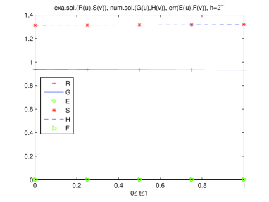
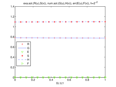
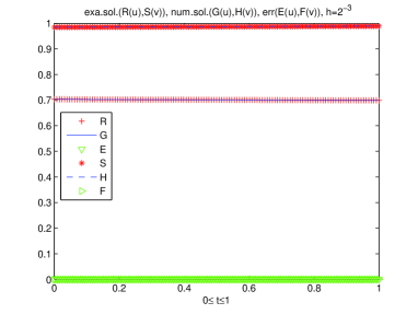
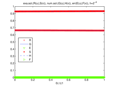
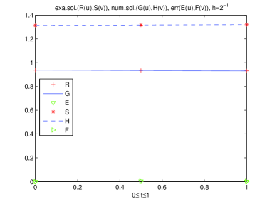
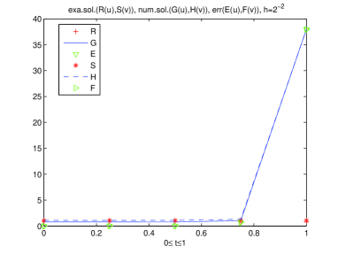
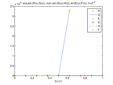
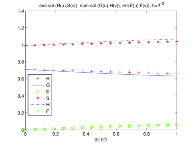
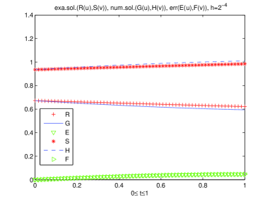
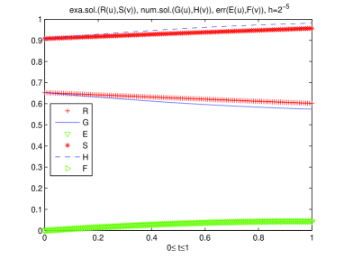
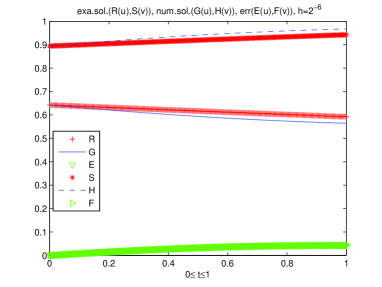
In the numerical tests, we assume that the mesh size h{12,122,123,124,125,126,127,128}121superscript221superscript231superscript241superscript251superscript261superscript271superscript28h\in\{\frac{1}{2},\frac{1}{2^{2}},\frac{1}{2^{3}},\frac{1}{2^{4}},\frac{1}{2^{5}},\frac{1}{2^{6}},\frac{1}{2^{7}},\frac{1}{2^{8}}\} and time step k{122,123,124,125,126,127,128,129,12101211}𝑘1superscript221superscript231superscript241superscript251superscript261superscript271superscript281superscript291superscript2101superscript211k\in\{\frac{1}{2^{2}},\frac{1}{2^{3}},\frac{1}{2^{4}},\frac{1}{2^{5}},\frac{1}{2^{6}},\frac{1}{2^{7}},\frac{1}{2^{8}},\frac{1}{2^{9}},\frac{1}{2^{10}}\frac{1}{2^{11}}\}. Furthermore, we compute the error estimates: |E(ϕ)|L2(0,T;L2),subscriptnorm𝐸italic-ϕsuperscript𝐿20𝑇superscript𝐿2\||E(\phi)|\|_{L^{2}(0,T;L^{2})}, |E(ϕ)|L(0,T;L2)subscriptnorm𝐸italic-ϕsuperscript𝐿0𝑇superscript𝐿2\||E(\phi)|\|_{L^{\infty}(0,T;L^{2})} and |E(ϕ)|L1(0,T;L2)subscriptnorm𝐸italic-ϕsuperscript𝐿10𝑇superscript𝐿2\||E(\phi)|\|_{L^{1}(0,T;L^{2})} (for ϕ=u,vitalic-ϕ𝑢𝑣\phi=u,v), associated with the three-level time-split scheme to demonstrate the efficiency and effectiveness of our method in two-dimensional case (stable, second order convergent in time and fourth order accurate in space). We plot the exact solution, computed solution and errors versus n.𝑛n. It comes from this analysis that the three-level time-split MacCormack method is more fast and efficient than a wide range of numerical schemes widely studied in the literature. Finally, Tables 111-444 suggest that the error terms O(kβ)+O(hθ)𝑂superscript𝑘𝛽𝑂superscript𝜃O(k^{\beta})+O(h^{\theta}) are dominated by the h-terms O(hθ)𝑂superscript𝜃O(h^{\theta}) (k𝑘k-terms O(kβ)𝑂superscript𝑘𝛽O(k^{\beta})). Thus, the numbers θ𝜃\theta (respectively β𝛽\beta) can be used to estimate the corresponding convergence rate with respect to hh (respectively, k𝑘k). Define the norms for the numerical solution ϕ,italic-ϕ\phi, the exact one ϕ¯,¯italic-ϕ\overline{\phi}, and the errors E(ϕ),𝐸italic-ϕE(\phi), as follows

|ϕ|L2(0,T;L2)=[kn=0𝑁ϕnLf22]12; |ϕ¯|L2(0,T;L2)=[kn=0𝑁ϕ¯nLf22]12;formulae-sequencesubscriptnormitalic-ϕsuperscript𝐿20𝑇superscript𝐿2superscriptdelimited-[]𝑘𝑛0𝑁superscriptsubscriptnormsuperscriptitalic-ϕ𝑛superscriptsubscript𝐿𝑓2212 subscriptnorm¯italic-ϕsuperscript𝐿20𝑇superscript𝐿2superscriptdelimited-[]𝑘𝑛0𝑁superscriptsubscriptnormsuperscript¯italic-ϕ𝑛superscriptsubscript𝐿𝑓2212\||\phi|\|_{L^{2}(0,T;L^{2})}=\left[k\underset{n=0}{\overset{N}{\sum}}\|\phi^{n}\|_{L_{f}^{2}}^{2}\right]^{\frac{1}{2}};\text{\,\,}\||\overline{\phi}|\|_{L^{2}(0,T;L^{2})}=\left[k\underset{n=0}{\overset{N}{\sum}}\|\overline{\phi}^{n}\|_{L_{f}^{2}}^{2}\right]^{\frac{1}{2}};
|E(ϕ)|L2(0,T;L2)=[kn=0𝑁ϕnϕ¯nLf22]12; |E(ϕ)|L1(0,T;L2)=kn=0𝑁ϕnϕ¯nLf2;formulae-sequencesubscriptnorm𝐸italic-ϕsuperscript𝐿20𝑇superscript𝐿2superscriptdelimited-[]𝑘𝑛0𝑁superscriptsubscriptnormsuperscriptitalic-ϕ𝑛superscript¯italic-ϕ𝑛superscriptsubscript𝐿𝑓2212 subscriptnorm𝐸italic-ϕsuperscript𝐿10𝑇superscript𝐿2𝑘𝑛0𝑁subscriptnormsuperscriptitalic-ϕ𝑛superscript¯italic-ϕ𝑛superscriptsubscript𝐿𝑓2\||E(\phi)|\|_{L^{2}(0,T;L^{2})}=\left[k\underset{n=0}{\overset{N}{\sum}}\|\phi^{n}-\overline{\phi}^{n}\|_{L_{f}^{2}}^{2}\right]^{\frac{1}{2}};\text{\,\,}\||E(\phi)|\|_{L^{1}(0,T;L^{2})}=k\underset{n=0}{\overset{N}{\sum}}\|\phi^{n}-\overline{\phi}^{n}\|_{L_{f}^{2}};

and

|E(ϕ)|L(0,T;L2)=max0nNϕnϕ¯nLf2.subscriptnorm𝐸italic-ϕsuperscript𝐿0𝑇superscript𝐿20𝑛𝑁subscriptnormsuperscriptitalic-ϕ𝑛superscript¯italic-ϕ𝑛superscriptsubscript𝐿𝑓2\||E(\phi)|\|_{L^{\infty}(0,T;L^{2})}=\underset{0\leq n\leq N}{\max}\|\phi^{n}-\overline{\phi}^{n}\|_{L_{f}^{2}}.

\bullet Test. Consider ΩΩ\Omega be the unit square (0,1)2superscript012(0,1)^{2} and T=1,𝑇1T=1, be the final time. The examples compare the numerical solutions with the exact ones to verify whether the proposed method leads to high accuracy. We assume that the Reynolds number R{2,64},𝑅264R\in\{2,64\}, such that the exact solutions u¯¯𝑢\overline{u} and v¯¯𝑣\overline{v} taken in [10] are given by

u¯(x,y,t)=14[3(1+exp(R(t4x+4y)/32))1],¯𝑢𝑥𝑦𝑡14delimited-[]3superscript1𝑅𝑡4𝑥4𝑦321\overline{u}(x,y,t)=\frac{1}{4}\left[3-\left(1+\exp\left(R(-t-4x+4y)/32\right)\right)^{-1}\right],
v¯(x,y,t)=14[3+(1+exp(R(t4x+4y)/32))1].¯𝑣𝑥𝑦𝑡14delimited-[]3superscript1𝑅𝑡4𝑥4𝑦321\overline{v}(x,y,t)=\frac{1}{4}\left[3+\left(1+\exp\left(R(-t-4x+4y)/32\right)\right)^{-1}\right].

The initial and boundary conditions are determined by this solution. We recall that the mesh size and time step: h{12,122,123,124,125,126,127,128}121superscript221superscript231superscript241superscript251superscript261superscript271superscript28h\in\{\frac{1}{2},\frac{1}{2^{2}},\frac{1}{2^{3}},\frac{1}{2^{4}},\frac{1}{2^{5}},\frac{1}{2^{6}},\frac{1}{2^{7}},\frac{1}{2^{8}}\} and k{122,123,124,125,126,127,128,129,1210,1211}.𝑘1superscript221superscript231superscript241superscript251superscript261superscript271superscript281superscript291superscript2101superscript211k\in\{\frac{1}{2^{2}},\frac{1}{2^{3}},\frac{1}{2^{4}},\frac{1}{2^{5}},\frac{1}{2^{6}},\frac{1}{2^{7}},\frac{1}{2^{8}},\frac{1}{2^{9}},\frac{1}{2^{10}},\frac{1}{2^{11}}\}.

Tables 1,2. Analysis of convergence rate O(hθ+Δtβ)𝑂superscript𝜃Δsuperscript𝑡𝛽O(h^{\theta}+\Delta t^{\beta}) for the three-level time-split MacCormack under the time step restriction (12)12(\ref{11**}), that is, 2R1kh212superscript𝑅1𝑘superscript21\frac{2R^{-1}k}{h^{2}}\leq 1, for low Reynolds number (for example, R=2𝑅2R=2), varying time step k=Δt𝑘Δ𝑡k=\Delta t and mesh grid h=Δx=ΔyΔ𝑥Δ𝑦h=\Delta x=\Delta y.

Table 1. k=R2h2=h2𝑘𝑅2superscript2superscript2k=\frac{R}{2}h^{2}=h^{2}.

hh |E(u)|L2subscriptnorm𝐸𝑢superscript𝐿2\||E(u)|\|_{L^{2}} |E(v)|L2subscriptnorm𝐸𝑣superscript𝐿2\||E(v)|\|_{L^{2}} |E(u)|Lsubscriptnorm𝐸𝑢superscript𝐿\||E(u)|\|_{L^{\infty}} |E(v)|Lsubscriptnorm𝐸𝑣superscript𝐿\||E(v)|\|_{L^{\infty}} |E(u)|L1subscriptnorm𝐸𝑢superscript𝐿1\||E(u)|\|_{L^{1}} |E(v)|L1subscriptnorm𝐸𝑣superscript𝐿1\||E(v)|\|_{L^{1}}
21superscript212^{-1} 7.391×1047.391superscript1047.391\times 10^{-4} 7.391×1047.391superscript1047.391\times 10^{-4} 7.926×1047.926superscript1047.926\times 10^{-4} 7.926×1047.926superscript1047.926\times 10^{-4} 7.316×1047.316superscript1047.316\times 10^{-4} 7.316×1047.316superscript1047.316\times 10^{-4}
22superscript222^{-2} 4.285×1044.285superscript1044.285\times 10^{-4} 4.285×1044.285superscript1044.285\times 10^{-4} 4.537×1044.537superscript1044.537\times 10^{-4} 4.537×1044.537superscript1044.537\times 10^{-4} 4.248×1044.248superscript1044.248\times 10^{-4} 4.248×1044.248superscript1044.248\times 10^{-4}
23superscript232^{-3} 3.671×1043.671superscript1043.671\times 10^{-4} 3.671×1043.671superscript1043.671\times 10^{-4} 3.957×1043.957superscript1043.957\times 10^{-4} 3.957×1043.957superscript1043.957\times 10^{-4} 3.594×1043.594superscript1043.594\times 10^{-4} 3.594×1043.594superscript1043.594\times 10^{-4}
24superscript242^{-4} 3.647×1043.647superscript1043.647\times 10^{-4} 3.647×1043.647superscript1043.647\times 10^{-4} 3.938×1043.938superscript1043.938\times 10^{-4} 3.938×1043.938superscript1043.938\times 10^{-4} 3.566×1043.566superscript1043.566\times 10^{-4} 3.566×1043.566superscript1043.566\times 10^{-4}


Table 2. k=h𝑘k=h.

hh |E(u)|L2subscriptnorm𝐸𝑢superscript𝐿2\||E(u)|\|_{L^{2}} |E(v)|L2subscriptnorm𝐸𝑣superscript𝐿2\||E(v)|\|_{L^{2}} |E(u)|Lsubscriptnorm𝐸𝑢superscript𝐿\||E(u)|\|_{L^{\infty}} |E(v)|Lsubscriptnorm𝐸𝑣superscript𝐿\||E(v)|\|_{L^{\infty}} |E(u)|L1subscriptnorm𝐸𝑢superscript𝐿1\||E(u)|\|_{L^{1}} |E(v)|L1subscriptnorm𝐸𝑣superscript𝐿1\||E(v)|\|_{L^{1}}
21superscript212^{-1} 0.00270.00270.0027 0.00270.00270.0027 0.00320.00320.0032 0.00320.00320.0032 0.00270.00270.0027 0.00270.00270.0027
22superscript222^{-2} 18.982118.982118.9821 18.982118.982118.9821 37.957937.957937.9579 37.957937.957937.9579 9.66909.66909.6690 9.66909.66909.6690
23superscript232^{-3} NaN NaN Inf Inf NaN NaN

Table 1 and Figure 1 suggest that under time step restriction (12)12(\ref{11**}), the proposed numerical scheme is stable, second order convergent in time and fourth order accurate in space, while Table 2 and Figures 2-3 indicate that when the time step constraint (12)12(\ref{11**}) is not satisfied, the considered algorithm is neither stable nor convergent.

Tables 3,4. Convergence rate O(hθ+Δtβ)𝑂superscript𝜃Δsuperscript𝑡𝛽O(h^{\theta}+\Delta t^{\beta}) for the three-level time-split MacCormack under time step restriction (51)51(\ref{44}) (that is, k34h1superscript𝑘341\frac{k^{\frac{3}{4}}}{h}\leq 1), for high Reynolds numbers (for instance, R=64𝑅64R=64), with varying time step k=Δt𝑘Δ𝑡k=\Delta t and mesh grid h=Δx=ΔyΔ𝑥Δ𝑦h=\Delta x=\Delta y.

Table 3. k=14hh43𝑘14superscript43k=\frac{1}{4}h\leq h^{\frac{4}{3}}.

hh |E(u)|L2subscriptnorm𝐸𝑢superscript𝐿2\||E(u)|\|_{L^{2}} |E(v)|L2subscriptnorm𝐸𝑣superscript𝐿2\||E(v)|\|_{L^{2}} |E(u)|Lsubscriptnorm𝐸𝑢superscript𝐿\||E(u)|\|_{L^{\infty}} |E(v)|Lsubscriptnorm𝐸𝑣superscript𝐿\||E(v)|\|_{L^{\infty}} |E(u)|L1subscriptnorm𝐸𝑢superscript𝐿1\||E(u)|\|_{L^{1}} |E(v)|L1subscriptnorm𝐸𝑣superscript𝐿1\||E(v)|\|_{L^{1}}
23superscript232^{-3} 3.9500×1023.9500superscript1023.9500\times 10^{-2} 3.9500×1023.9500superscript1023.9500\times 10^{-2} 5.8900×1025.8900superscript1025.8900\times 10^{-2} 5.8900×1025.8900superscript1025.8900\times 10^{-2} 3.5500×1023.5500superscript1023.5500\times 10^{-2} 3.5500×1023.5500superscript1023.5500\times 10^{-2}
24superscript242^{-4} 3.3500×1023.3500superscript1023.3500\times 10^{-2} 3.3500×1023.3500superscript1023.3500\times 10^{-2} 4.6400×1024.6400superscript1024.6400\times 10^{-2} 4.6400×1024.6400superscript1024.6400\times 10^{-2} 3.0400×1023.0400superscript1023.0400\times 10^{-2} 3.0400×1023.0400superscript1023.0400\times 10^{-2}
25superscript252^{-5} 3.2200×1023.2200superscript1023.2200\times 10^{-2} 3.2200×1023.2200superscript1023.2200\times 10^{-2} 4.3800×1024.3800superscript1024.3800\times 10^{-2} 4.3800×1024.3800superscript1024.3800\times 10^{-2} 2.9400×1022.9400superscript1022.9400\times 10^{-2} 2.9400×1022.9400superscript1022.9400\times 10^{-2}
26superscript262^{-6} 3.1800×1023.1800superscript1023.1800\times 10^{-2} 3.1800×1023.1800superscript1023.1800\times 10^{-2} 4.3000×1024.3000superscript1024.3000\times 10^{-2} 4.3000×1024.3000superscript1024.3000\times 10^{-2} 2.9000×1022.9000superscript1022.9000\times 10^{-2} 2.9000×1022.9000superscript1022.9000\times 10^{-2}
27superscript272^{-7} 3.1600×1023.1600superscript1023.1600\times 10^{-2} 3.1600×1023.1600superscript1023.1600\times 10^{-2} 4.2700×1024.2700superscript1024.2700\times 10^{-2} 4.2700×1024.2700superscript1024.2700\times 10^{-2} 2.8800×1022.8800superscript1022.8800\times 10^{-2} 2.8800×1022.8800superscript1022.8800\times 10^{-2}


Table 4. k=h>h43𝑘superscript43k=h>h^{\frac{4}{3}}.

k𝑘k |E(u)|L2subscriptnorm𝐸𝑢superscript𝐿2\||E(u)|\|_{L^{2}} |E(v)|L2subscriptnorm𝐸𝑣superscript𝐿2\||E(v)|\|_{L^{2}} |E(u)|Lsubscriptnorm𝐸𝑢superscript𝐿\||E(u)|\|_{L^{\infty}} |E(v)|Lsubscriptnorm𝐸𝑣superscript𝐿\||E(v)|\|_{L^{\infty}} |E(u)|L1subscriptnorm𝐸𝑢superscript𝐿1\||E(u)|\|_{L^{1}} |E(v)|L1subscriptnorm𝐸𝑣superscript𝐿1\||E(v)|\|_{L^{1}}
23superscript232^{-3} 4.9400×1024.9400superscript1024.9400\times 10^{-2} 4.9400×1024.9400superscript1024.9400\times 10^{-2} 7.6100×1027.6100superscript1027.6100\times 10^{-2} 7.6100×1027.6100superscript1027.6100\times 10^{-2} 4.4200×1024.4200superscript1024.4200\times 10^{-2} 4.4200×1024.4200superscript1024.4200\times 10^{-2}
24superscript242^{-4} 3.8600×1023.8600superscript1023.8600\times 10^{-2} 3.8600×1023.8600superscript1023.8600\times 10^{-2} 5.3900×1025.3900superscript1025.3900\times 10^{-2} 5.3900×1025.3900superscript1025.3900\times 10^{-2} 3.5200×1023.5200superscript1023.5200\times 10^{-2} 3.5200×1023.5200superscript1023.5200\times 10^{-2}
25superscript252^{-5} 3.4200×1023.4200superscript1023.4200\times 10^{-2} 3.4200×1023.4200superscript1023.4200\times 10^{-2} 4.6400×1024.6400superscript1024.6400\times 10^{-2} 4.6400×1024.6400superscript1024.6400\times 10^{-2} 3.1300×1023.1300superscript1023.1300\times 10^{-2} 3.1300×1023.1300superscript1023.1300\times 10^{-2}
26superscript262^{-6} NaN NaN Inf Inf NaN NaN

Table 3 and Figure 4 indicate that for high Reynolds numbers and under time step restriction (12)12(\ref{11**}), the considered method is stable, second order convergent in both time and space, while Table 4 shows that the scheme is neither stable nor convergent for smallest mesh size hh, whenever the time step limitation (12)12(\ref{11**}) is not accomplished.

4 General conclusion and future works

In this paper, we have discussed the convergence rate of the three-level explicit time-split MacCormack algorithm for solving the two-dimensional time dependent nonlinear coupled Burgers’ equations (1)1(\ref{1}) subject to the initial and boundary conditions (2)2(\ref{2})-(3)3(\ref{3}). For low Reynolds numbers, the theoretical results have shown that the proposed algorithm is stable, second order convergent in time and fourth order accurate in space, while for large Reynolds numbers, the analysis has demonstrated that the considered method is second order convergent in time and space. All this analysis has been done under the time step requirement (12)12(\ref{11**}). The theoretical study is confirmed by a wide set of numerical experiments (Figures 1-4 and Tables 1-4). The numerical experiments also show that our method is: (a) more fast and efficient than a broad range of numerical schemes for solving the initial-boundary value problem (1)1(\ref{1})-(3)3(\ref{3}); (b) fast and robust tools for the integration of general systems of hyperbolic/parabolic PDEs. Unfortunately, we have observed from the numerical examples that the time-split MacCormack method is not too much efficient for solving high Reynolds number flows where the viscous region is very thin. The mesh size must be highly refined in order to accurately resolve the viscous regions. The small grid spacing leads to very small time steps and subsequently long computing times. Indeed, in the coarse-grid region, the three-level explicit time-split MacCormack approach can be applied, while in the fine-grid region, the following sequence of nonlinear operators can be used

(uijn+1vijn+1)=[Lx(k2m)Ly(km)Lx(k2m)]m(uijnvijn),matrixsuperscriptsubscript𝑢𝑖𝑗𝑛1superscriptsubscript𝑣𝑖𝑗𝑛1superscriptdelimited-[]subscript𝐿𝑥𝑘2𝑚subscript𝐿𝑦𝑘𝑚subscript𝐿𝑥𝑘2𝑚𝑚matrixsuperscriptsubscript𝑢𝑖𝑗𝑛superscriptsubscript𝑣𝑖𝑗𝑛\begin{pmatrix}u_{ij}^{n+1}\\ v_{ij}^{n+1}\\ \end{pmatrix}=\left[L_{x}\left(\frac{k}{2m}\right)L_{y}\left(\frac{k}{m}\right)L_{x}\left(\frac{k}{2m}\right)\right]^{m}\begin{pmatrix}u_{ij}^{n}\\ v_{ij}^{n}\\ \end{pmatrix},

where m𝑚m is the smallest integer satisfying inequality: max{2kmRh2,k34m34h}1.2𝑘𝑚𝑅superscript2superscript𝑘34superscript𝑚341\max\left\{\frac{2k}{mRh^{2}},\frac{k^{\frac{3}{4}}}{m^{\frac{3}{4}}h}\right\}\leq 1. Our future investigations will consider the last formula together with the three-level time-split MacCormack technique in the numerical solutions of two-dimensional unsteady viscous coupled Burgers’ equations (1)1(\ref{1})-(3)3(\ref{3}).

Acknowledgment. The author would like to thank the deanship of scientific research of Imam Muhammad Ibn Saud Islamic University (IMSIU) to financially support this work under the Grant No. 331203.

Stability and convergence of a three-level time-split MacCormack method: a=μ=1𝑎𝜇1a=\mu=1. Refer to caption Refer to caption Refer to caption Refer to caption

Figure 1: Graphs corresponding to a three-level time-split MacCormack method

Stability and convergence of a three-level time-split MacCormack method: a=μ=1𝑎𝜇1a=\mu=1. Refer to caption Refer to caption

Figure 2: Graphs corresponding to a three-level time-split MacCormack method

Stability and convergence of a three-level time-split MacCormack method: a=μ=1𝑎𝜇1a=\mu=1. Refer to caption

Figure 3: Graphs corresponding to a three-level time-split MacCormack method

Stability and convergence of a three-level time-split MacCormack method: a=μ=1𝑎𝜇1a=\mu=1. Refer to caption Refer to caption Refer to caption Refer to caption

Figure 4: Graphs corresponding to a three-level time-split MacCormack method

References

  • [1] F. A. Anderson, R. H. Pletcher, J. C. Tannehill. ”Computational fluid mechanics and Heat Transfer”. Second Edition, Taylor and Francis, New York, (1997).1997(1997).
  • [2] A. Bahadir. ”A fully implicit finite-difference scheme for two-dimensional Burgers’ equations”. Appl. Math. Comput., Vol. 137137137, (2003),2003(2003), pp. 131131131-137.137137.
  • [3] M. Basto, V. Semiao, F. Calheiros. ”Dynamics and synchronization of numerical solutions of the Burgers’ equation”. J. Comput. Appl. Math., Vol. 231231231, (2009),2009(2009), pp. 793793793-806.806806.
  • [4] M. Burgers. ”A mathematical model illustrating the theory of turbulence”. Adv. in Appl. Mech., Vol. 111, (1948),1948(1948), pp. 171171171-199.199199.
  • [5] M. Dehghan. ”Time-split procedures for the solution of the two-dimensional transport equations”. Kybernetes, Vol. 36(5/6)365636(5/6), (2007b),2007𝑏(2007b), pp. 791791791-805.805805.
  • [6] M. Dehghan, A. Hamidi, M. Shakourifar. ”The solution of coupled Burgers’ equations using adomain-pade technique”. Appl. Math. Comput., Vol. 189189189, (2007),2007(2007), pp. 103410341034-1047.10471047.
  • [7] M. Dehghan, R. Salehi. ”The chebyshev spectral viscosity method for the time dependent Eikonal equation”. Mathematical and Computer Modelling, Vol. 197197197, (2010),2010(2010), pp. 707070-86.8686.
  • [8] M. Dehghan, A. Ghesmati. ”Combination of meshless local weak and strong (MLWS) forms to solve the two-dimensional hyperbolic telegraph equation”. Engineering Analysis with Boundary Elements, Vol. 343434, (2010),2010(2010), pp. 324324324-336.336336.
  • [9] S. M. El-Sayed, D. Kaya. ”On the numerical solution of the system of two-dimensional Burgers’ equations by decomposition method”. Appl. Math. Comput., Vol. 158158158, (2004),2004(2004), pp. 101101101-109.109109.
  • [10] C. A. J. Fletcher. ”Generating exact solution of the two-dimensional Burgers’ equations”. Int. J. Numer. Meth. Fluids, Vol. 333, (1983b),1983𝑏(1983b), pp. 213213213-216.216216.
  • [11] C. A. J. Fletcher. ”A comparison of finite element and finite difference solution of the one and two-dimensional Burgers’ equations”. J. Comput. Phys., Vol. 515151, (1983a),1983𝑎(1983a), pp. 159159159-188.188188.
  • [12] O. Goyon. ”Multilevel schemes fpr solving unsteady equations”. Int. J. Numer. Meth. Fluids, Vol. 222222, (1996),1996(1996), pp. 937937937-959.959959.
  • [13] H. Khater, R. S. Temsah, M. M. Hassan. ”A chebyshev spectral collocation method for solving Burgers’-type equations”. J. Comput. Appl. Math., Vol. 222(2)2222222(2), (2008),2008(2008), pp. 333333333-350.350350.
  • [14] S. Kutluay. A. Esen, I. Dag. ”Numerical solution of the Burgers’ equation by the least-squares quadratic B-spline finite element method”. J. Comput. Appl. Math., Vol. 167167167, (2004),2004(2004), pp. 212121-33.3333.
  • [15] P. D. Lax, B. Wendroff. ”Systems of conservation laws”, Comm. Pure &\& Appl. Math. 131313 (1960)1960(1960) 217217217-237.237237.
  • [16] W. Liao. ”A fourth-order finite-difference method for solving the system of two-dimensional Burgers’ equations”. Int. J. Numer. Meth. Fluids, Vol. 64(5)64564(5), (2009),2009(2009), pp. 565565565-590.590590.
  • [17] R. W. MacCormack. ”An efficient numerical method for solving the time-dependent compressible Navier-Stokes equations at high Reynolds numbers”, NASA TM (1976)1976(1976) 737373-129.129129.
  • [18] R. W. MacCormack. ”A numerical method for solving the equations of compressible viscous-flows”, AIAA paper 818181-0110,01100110, St. Louis, Missouri (1981).1981(1981).
  • [19] R. W. MacCormack, A. J. Paullay. ”Computational efficiency achieved by time splitting of finite difference operators”, AIAA paper 727272-154,154154, San Diego, California (1972).1972(1972).
  • [20] R. C. Mittal, R. Jiwari. ”Zakharov-Kuznetsov-Burgers’ equation for dust ion acoustic waves”. Chaos Solitons fractals, Vol. 363636, (2008),2008(2008), pp. 628628628-634.634634.
  • [21] W. M. Moslem, R. Sabry. ”A fourth-order finite-difference method for solving the system of two-dimensional Burgers’ equations”. Int. J. Numer. Meth. Fluids, Vol. 64(5)64564(5), (2009),2009(2009), pp. 565565565-590.590590.
  • [22] F. T. Namio, E. Ngondiep, R. Ntchantcho, J. C. Ntonga. ”Mathematical models of complete shallow water equations with source terms, stability analysis of Lax-Wendroff scheme”, J. Theor. Comput. Sci., Vol. 2(132)21322(132) (2015).2015(2015).
  • [23] E. Ngondiep. ”Stability analysis of MacCormack rapid solver method for evolutionary Stokes-Darcy problem”, J. Comput. Appl. Math. 345(2019)3452019345(2019), 269269269-285285285, 171717 pages.
  • [24] E. Ngondiep. ”A three-level explicit time-split MacCormack method for 222D nonlinear reaction-diffusion equations”, preprint available online from http://arxiv.org/abs/1903.10877, 2019.
  • [25] E. Ngondiep. ”Long Time Stability and Convergence Rate of MacCormack Rapid Solver Method for Nonstationary Stokes-Darcy Problem”, Comput. Math. Appl., Vol 757575, (2018)2018(2018), 366336633663-3684,36843684, 222222 pages.
  • [26] E. Ngondiep. ”An efficient three-level explicit time-split method for solving 222D heat conduction equations”, submitted.
  • [27] E. Ngondiep. ”Long time unconditional stability of a two-level hybrid method for nonstationary incompressible Navier-Stokes equations”, J. Comput. Appl. Math. 345(2019)3452019345(2019), 501501501-514514514, 141414 pages.
  • [28] E. Ngondiep. ”Asymptotic growth of the spectral radii of collocation matrices approximating elliptic boundary problems”, Int. J. Appl. Math. Comput., 4(2012)420124(2012), 199199199-219,219219, 202020 pages.
  • [29] E. Ngondiep. ”A novel three-level time-split MacCormack scheme for two-dimensional evolutionary linear convection-diffusion-reaction equation with source term”, submitted.
  • [30] E. Ngondiep. ”Error estimate of MacCormack rapid solver method for 2D incompressible Navier-Stokes problems”, preprint available online from http://arxiv.org/abs/1903.10857, 2019.
  • [31] E. Ngondiep. ”Analysis of stability and convergence rate of a three-level time-split method for two-dimensional unsteady convection-diffusion equation”, submitted.
  • [32] E. Ngondiep. ”A new three-level time-split explicit method for two-dimensional nonlinear unsteady convection-diffusion-reaction equation”, submitted.
  • [33] E. Ngondiep, R. Alqahtani and J. C. Ntonga. ”Stability analysis and convergence rate of MacCormack scheme for complete shallow water equations with source terms”, preprint available online from http://arxiv.org/abs/1903.11104, 2019.
  • [34] A. Rashid, A. I. B. M. Ismail. ”A Fourier pseudospectral method for solving coupled Burgers’ equations”. Comput. Meth. Appl. Math., Vol. 9(4),949(4), (2009),2009(2009), pp. 412412412-420.420420.
  • [35] M. M. Rashidi, E. Erfani. ”New analytical method for solving two-dimensional Burgers’ and nonlinear heat transfer equations and comparison with HAM”. Comput. Phys. Commun., Vol. 180180180, (2009),2009(2009), pp. 153915391539-1544.15441544.
  • [36] H. Zhu, H. Shu, M. Ding. ”Numerical solutions of two-dimensional Burgers’ equations by discrete Adomain decomposition method”. Comput. Math. Appl., Vol. 606060, (2010),2010(2010), pp. 840840840-848.848848.