DESY 19-092 HU-EP-19/13 P3H-19-012 TTP19-014
Top quark mass dependence of the Higgs-gluon form factor at three loops

Abstract

We compute three-loop corrections to the Higgs-gluon form factor, incorporating the top quark mass dependence. Our method is based on the combination of expansions around the top threshold and for large top quark mass, using conformal mapping and Padé approximation to describe the form factor over the full kinematic range.

1 Introduction

The precise measurement of the properties of the Higgs boson, in particular the coupling strength to other particles and to itself, will be among the main focuses in particle physics in the coming years. The success of this enterprise crucially depends on the accuracy of the predictions provided by the theory community.

A quantity which is available to high perturbative order is the total cross section for the production of a Higgs boson at the Large Hadron Collider (LHC). For a comprehensive collection of relevant works we refer to Ref. [1], but we remark here that QCD corrections including the exact dependence on the top quark mass, $m_{t}$, have been available at next-to-leading order (NLO) for about 25 years [2]. At higher orders only approximate results are available; at NNLO the infinite top quark mass results from Refs. [3, 4, 5] have been complemented by power-suppressed terms in the inverse top quark mass in [6, 7, 8, 9]. The N³LO result has been obtained in the $m_{t}\to\infty$ limit in [10, 11].

In Ref. [1] several sources of uncertainties have been identified for the prediction of the total cross section. Among them is that of the exact top quark mass dependence of the NNLO corrections which has been estimated to be 1%. In this paper we provide results for the Higgs-gluon form factor at three-loop order which constitutes the virtual corrections to the production cross section. Thus the findings of this paper help to eliminate the aforementioned uncertainty to a large extent. The Higgs-gluon form factor is also an important ingredient for processes where the relevant energy in the fermion loops reaches values close to or above the top quark threshold and the infinite top quark mass limit cannot be applied anymore. This concerns, e.g., Higgs boson pair production via $gg\to H^{\star}\to HH$ or the measurement of the Higgs boson width from off-shell production of $Z$ boson pairs in gluon fusion via $gg\to H^{\star}\to ZZ$ [12]. The exact dependence on the fermion mass in the loop is also important for numerous theories beyond the Standard Model, which often contain additional heavier Higgs bosons.

At two-loop order exact results for the form factor are known from Refs. [2, 13, 14, 15]. However, at three loops only expansions for large top quark mass [16, 17] and non-analytic terms in the expansion around the top threshold up to ${\cal O}(1-z)$ [18] are known, where

$$z=\frac{\hat{s}}{4m_{t}^{2}}$$ (1)

with $\sqrt{\hat{s}}$ being the partonic center-of-mass energy. For later convenience we also introduce $\bar{z}=1-z$. In the next section we describe our method which we use to combine these expansions in order to obtain results for the form factor valid for all space- and time-like momentum transfers. In Section 3 we discuss our results and Section 4 contains a brief summary.

2 Method

The method we use for the construction of the top quark mass dependence of the Higgs-gluon form factor is based on the efficient combination of information from the large top quark mass expansion (LME) ($z\to 0$) and knowledge from the threshold where $\hat{s}\approx 4m_{t}^{2}$ ($z\to 1$), using conformal mapping and Padé approximation. The procedure was developed in Ref. [19] (see also [20, 21]) in order to compute a certain class of four-loop contributions to the muon anomalous magnetic moment. In Refs. [22, 23] the method was extended to QCD corrections with the aim to compute NNLO correction to the total cross section $\sigma(e^{+}e^{-}\to\mbox{hadrons})$. A further refinement of the method has been developed in Refs. [24, 25] where order $\alpha_{s}^{3}$ corrections to $\sigma(e^{+}e^{-}\to\mbox{hadrons})$ have been computed. In these references additional parameters were introduced which allow one to generate a larger number of Padé approximations and thus obtain more reliable uncertainty estimates. The systematic improvement of the Padé approximations when increasing the number of input terms has been studied in Ref. [26]. In Ref. [18] the method has been used to obtain two-loop corrections for the three form factors relevant for Higgs boson pair production.

In the following we briefly describe the application of this method to the form factor entering the interaction of a Higgs boson and two gluons. We parameterize the corresponding amplitude as

$${\cal A}^{\mu\nu}_{ab}(gg\to H) = \delta_{ab}\frac{y_{t}}{2\sqrt{2}m_{t}}\frac{\alpha_{s}}{\pi}T_{F}\left(q_{1}\cdot q_{2}g^{\mu\nu}-q_{1}^{\nu}q_{2}^{\mu}\right)F_{\triangle}(z)\,,$$ (2)

where $q_{1}$ and $q_{2}$ are the external momenta of the gluons with polarization vectors $\varepsilon^{\mu}(q_{1})$ and $\varepsilon^{\nu}(q_{2})$, respectively. $y_{t}=\sqrt{2}m_{t}/v$ is the top quark Yukawa coupling, $v$ is the vacuum expectation value, $a$ and $b$ are adjoint colour indices, $T_{F}=1/2$ and $\hat{s}=(q_{1}+q_{2})^{2}=2q_{1}\cdot q_{2}$. It is convenient to define the perturbative expansion of $F_{\triangle}$ as

$$F_{\triangle} = F_{\triangle}^{(0)}+\frac{\alpha_{s}}{\pi}F_{\triangle}^{(1)}+\left(\frac{\alpha_{s}}{\pi}\right)^{2}F_{\triangle}^{(2)}+\cdots\,,$$ (3)

where $\alpha_{s}\equiv\alpha_{s}^{(5)}(\mu)$ is the strong coupling constant with five active flavours evaluated at the renomalization scale $\mu$. Sample Feynman diagrams contributing to ${\cal A}^{\mu\nu}_{ab}(gg\to H)$ up to three loops can be found in Figure 1.

Figure 1: One-, two- and three-loop Feynman diagrams contributing to $F_{\triangle}$. Solid, curly and dashed lines represent quarks, gluons and Higgs bosons, respectively.

The one-loop result, $F^{(0)}_{\triangle}$, is finite. At two-loop order we renormalize the gluon wave function and the top quark mass in the on-shell scheme and the strong coupling constant in the $\overline{\rm MS}$ scheme. Note that the ultra-violet renormalized form factor still contains infra-red divergences which cancel against contributions from real radiation, in order to form finite physical quantities. The structure of the infra-red divergences is universal and has been studied in detail in the literature [27]. In our case finite form factors are obtained via

$$F^{(1),\rm fin}_{\triangle} = F_{\triangle}^{(1)}-\frac{1}{2}I^{(1)}_{g}F_{\triangle}^{(0)}\,,$$

$$F^{(2),\rm fin}_{\triangle} = F_{\triangle}^{(2)}-\frac{1}{2}I^{(1)}_{g}F_{\triangle}^{(1)}-\frac{1}{4}I^{(2)}_{g}F_{\triangle}^{(0)}\,,$$ (4)

where $I^{(1)}_{g}$ and $I^{(2)}_{g}$ can be found in Refs. [27, 28]. In order to fix the notation we provide an explicit expression only for $I^{(1)}_{g}$ which is given by

$$I^{(1)}_{g} = {}-\left(\frac{\mu^{2}}{-\hat{s}-i\delta}\right)^{\epsilon}\frac{e^{\epsilon\gamma_{E}}}{\Gamma(1-\epsilon)}\frac{1}{\epsilon^{2}}\Big{[}C_{A}+2\epsilon\beta_{0}\Big{]}\,,$$ (5)

with $\beta_{0}=(11C_{A}-4T_{F}n_{l})/12$ where $C_{A}=3$, $T_{F}=1/2$ and $n_{l}$ is the number of massless quarks. We work in $d=4-2\epsilon$ dimensions and assume that $\delta$ is an infinitesimal small parameter. We apply the method described below to $F^{(1),\rm fin}_{\triangle}$ and $F^{(2),\rm fin}_{\triangle}$.

In the following we briefly discuss the input for the limits $z\to 0$ and $z\to 1$ used for the construction of the Padé approximants. For the renormalization scale we choose $\mu^{2}=-\hat{s}$ since the $\mu$ dependence can easily be reconstructed from the one- and two-loop expressions, which are known exactly, see Ref. [29]. Furthermore, we set all colour factors to their numerical values and only keep $n_{l}$ as a parameter. The large-$m_{t}$ expansion of the three-loop form factor up to order $z^{4}$ has been computed in Ref. [16, 17] and the $z^{5}$ and $z^{6}$ terms are available from Ref. [29]. The analytic expressions read

$$F_{\triangle}^{(0)} = \frac{4}{3}+\frac{14}{45}z+\frac{8}{63}z^{2}+\frac{104}{1575}z^{3}+\frac{2048}{51975}z^{4}+\frac{4864}{189189}z^{5}+\frac{512}{28665}z^{6}+{\cal O}(z^{7})\,,$$

$$\vphantom{\Bigg{[}}F_{\triangle}^{(1),\rm fin} = \frac{11}{3}+\frac{1237}{810}z+\frac{35726}{42525}z^{2}+\frac{157483}{297675}z^{3}+\frac{2546776}{7016625}z^{4}+\frac{194849538824}{737482370625}z^{5}$$

$$\mbox{}+\frac{385088204192}{1917454163625}z^{6}+{\cal O}(z^{7})\,,$$

$$\vphantom{\Bigg{[}}F_{\triangle}^{(2),\rm fin} = -\frac{253\zeta(3)}{24}+\frac{3941}{108}+\frac{19\pi^{2}}{12}+\frac{\pi^{4}}{96}+\frac{19}{12}L_{s}$$ (6)

$$\mbox{}+n_{l}\Bigg{(}-\frac{17\zeta(3)}{36}-\frac{3239}{648}-\frac{47\pi^{2}}{432}+\frac{4}{9}L_{s}\Bigg{)}+n_{l}^{2}\frac{\pi^{2}}{648}$$

$$\mbox{}+\Bigg{[}\frac{9290881\zeta(3)}{103680}-\frac{44326367}{466560}+\frac{623\pi^{2}}{1080}+\frac{7\pi^{4}}{2880}+\frac{28}{405}\pi^{2}\log(2)+\frac{8261}{3240}L_{s}$$

$$\mbox{}+n_{l}\Bigg{(}-\frac{119\zeta(3)}{1080}-\frac{107087}{291600}-\frac{259\pi^{2}}{4320}-\frac{169}{1080}L_{s}\Bigg{)}+n_{l}^{2}\frac{7\pi^{2}}{19440}\Bigg{]}z$$

$$\mbox{}+\Bigg{[}\frac{7037623781\zeta(3)}{69672960}-\frac{82500975779}{731566080}+\frac{121\pi^{2}}{378}+\frac{\pi^{4}}{1008}+\frac{32}{567}\pi^{2}\log(2)$$

$$\mbox{}+\frac{253549}{170100}L_{s}+n_{l}\Bigg{(}-\frac{17\zeta(3)}{378}-\frac{6385481}{53581500}-\frac{25\pi^{2}}{648}-\frac{4133}{36450}L_{s}\Bigg{)}$$

$$\mbox{}+n_{l}^{2}\frac{\pi^{2}}{6804}\Bigg{]}z^{2}+\Bigg{[}\frac{650760513719\zeta(3)}{412876800}-\frac{1740869750908152049}{921773260800000}+\frac{221\pi^{2}}{1050}$$

$$\mbox{}+\frac{13\pi^{4}}{25200}+\frac{208\pi^{2}\log(2)}{4725}+\frac{804644}{826875}L_{s}+n_{l}\Bigg{(}-\frac{221\zeta(3)}{9450}-\frac{6383750249}{112521150000}$$

$$\mbox{}-\frac{3107\pi^{2}}{113400}-\frac{1147037}{14883750}L_{s}\Bigg{)}+n_{l}^{2}\frac{13\pi^{2}}{170100}\Bigg{]}z^{3}$$

$$\mbox{}+\Bigg{[}\frac{193543938976537\zeta(3)}{37158912000}-\frac{6978205934887756008911}{1115345645568000000}+\frac{4736\pi^{2}}{31185}+\frac{16\pi^{4}}{51975}$$

$$\mbox{}+\frac{16384\pi^{2}\log(2)}{467775}+\frac{33498106}{49116375}L_{s}+n_{l}\Bigg{(}-\frac{2176\zeta(3)}{155925}-\frac{2197298833}{72937816875}$$

$$\mbox{}-\frac{3232\pi^{2}}{155925}-\frac{20932}{382725}L_{s}\Bigg{)}+n_{l}^{2}\frac{64\pi^{2}}{1403325}\Bigg{]}z^{4}$$

$$\mbox{}+\Bigg{[}\frac{2460310706266276921\zeta(3)}{81155063808000}-\frac{159929147625953730170902566067}{4389031448658778521600000}$$

$$\mbox{}+\frac{9424\pi^{2}}{81081}+\frac{38\pi^{4}}{189189}+\frac{48640\pi^{2}\log(2)}{1702701}+\frac{945911804923}{1877227852500}L_{s}+n_{l}\Bigg{(}-\frac{5168\zeta(3)}{567567}$$

$$\mbox{}-\frac{22552503119716043}{1395235522161731250}-\frac{27892\pi^{2}}{1702701}-\frac{48324340168}{1191317675625}L_{s}\Bigg{)}+n_{l}^{2}\frac{152\pi^{2}}{5108103}\Bigg{]}z^{5}$$

$$\mbox{}+\Bigg{[}\frac{15128773883548934558969\zeta(3)}{114266329841664000}+\frac{2656\pi^{2}}{28665}+\frac{4\pi^{4}}{28665}+\frac{2048\pi^{2}\log(2)}{85995}$$

$$\mbox{}\vphantom{\Bigg{[}}-\frac{13560383230749413568271118392175429}{85205730523295753699328000000}+\frac{339242844181}{871570074375}L_{s}$$

$$\mbox{}\vphantom{\Bigg{[}}+n_{l}\Bigg{(}-\frac{544\zeta(3)}{85995}-\frac{2085146760850288}{259115168401464375}-\frac{3448\pi^{2}}{257985}-\frac{35895528824}{1150472498175}L_{s}\Bigg{)}$$

$$\mbox{}+n_{l}^{2}\frac{16\pi^{2}}{773955}\Bigg{]}z^{6}+{\cal O}(z^{7})\,,$$

where $L_{s}=\log(-4z-i0)$ and $\zeta(n)$ is the Riemann zeta function.

The expansion of the three-loop form factor around threshold was considered in Ref. [18] in the effective theory of Non-Relativistic QCD (NRQCD). We briefly outline the approach and refer to [18] for details.

Within NRQCD, the leading contributions to the triangle form factor near threshold can be written schematically as

$$F_{\triangle}(z)\mathop{\asymp}\limits^{z\to 1}C_{gg\to t\bar{t}}C_{t\bar{t}\to H}G_{P}(z)\,,$$ (7)

where the symbol “$\asymp$” indicates that terms analytic in $(1-z)$ have been dropped on the right-hand side. The relativistic short-distance corrections to top pair production and annihilation are absorbed into the matching coefficients $C_{gg\to t\bar{t}},C_{t\bar{t}\to H}$ and the propagation of the intermediate non-relativistic $t\bar{t}$ pair is described by the Coulomb resummed $P$-wave Green function $G_{P}(z)$ [30]. Expanding Eq. (7) in $\alpha_{s}$ yields the perturbative coefficients of the form factor. An explicit result for the three-loop form factor is given in Eq. (50) of [18]. For convenience we reproduce the analytic expression together with the one- and two-loop results which are given by

$$F_{\triangle}^{(0)}\mathop{\asymp}\limits^{z\to 1} \,2\pi(1-z)^{3/2}+\frac{13\pi}{3}(1-z)^{5/2}+\mathcal{O}\left((1-z)^{7/2}\right)\,,$$

$$F_{\triangle}^{(1),\text{fin}}\mathop{\asymp}\limits^{z\to 1} \,\frac{4\pi^{2}}{3}(1-z)\log(1-z)-\frac{\pi}{36}\left(124+15\pi^{2}\right)(1-z)^{3/2}+\frac{8\pi^{2}}{9}(1-z)^{2}\log(1-z)$$

$$+\frac{\pi}{216}\Big{[}2252-117\pi^{2}-2112\log(2)-672\log(1-z)\Big{]}(1-z)^{5/2}$$

$$-\frac{28\pi^{2}}{45}(1-z)^{3}\log(1-z)+\mathcal{O}\left((1-z)^{7/2}\right)\,,$$

$$F_{\triangle}^{(2),\text{fin}} \mathop{\asymp}\limits^{z\to 1}-\frac{8\pi^{3}}{27}\left(3+\pi^{2}\right)\sqrt{1-z}$$

$$+\frac{\pi^{2}}{54}\Big{[}\left(458-15\pi^{2}-44n_{l}{+(198-12n_{l})(L_{s}-2\ln 2)}\right)\log(1-z)$$

$$-(99-6n_{l})\log^{2}(1-z)\Big{]}(1-z)+\mathcal{O}\left((1-z)^{3/2}\right)\,.$$ (8)

The information provided in Eqs. (6) and (8) is used to construct approximations of the form factor. We first subtract the logarithmic contributions for $z\sim 1$ and define

$$\tilde{F}_{\triangle}=F_{\triangle}-F_{\triangle}^{\rm sub}\,,$$ (9)

where $F_{\triangle}^{\rm sub}$ is constructed to both be analytic for $|z|<1$ and to reproduce the threshold logarithms in Eq. (8), so that the threshold expansion of $\tilde{F}_{\triangle}$ is free of logarithms up to $(1-z)^{3/2}$. Such a subtraction function $F_{\triangle}^{\rm sub}$ can be obtained using the vacuum polarization as a building block, see [18] for details of the construction. For explicit examples for $F_{\triangle}^{\rm sub}$ we refer to the sample Padé approximants in the ancillary file [31]. Note that also in the limit $z\to 0$ $F_{\triangle}$ develops logarithmic divergences which manifest in the linear $L_{s}$ term in Eq. (6). Whereas in Ref. [23] these contributions are also subtracted, here we instead construct separate Padé approximants for the $L_{s}$-independent term and for the coefficient of $L_{s}$, as discussed in [18].

Next we apply a conformal mapping

$$z = \frac{4\omega}{(1+\omega)^{2}}\,,$$ (10)

to transform the $z$ plane into the interior of the unit circle in the $\omega$ plane; the time-like momentum regions $z\in[0,1]$ and $z\in[1,\infty]$ with $\mbox{Im}(z)>0$ are mapped to $\omega\in[0,1]$ and the upper semi-circle, respectively.

At this point we construct Padé approximants in the variable $\omega$. They have the form

$$[n/m](\omega)=\frac{\sum\limits_{i=0}^{n}a_{i}\omega^{i}}{1+\sum\limits_{j=1}^{m}b_{j}\omega^{j}}\,,$$ (11)

where $n+m$ is fixed by the number of input terms from the large top mass and threshold expansions. In our case we have seven terms for $z\to 0$ and one for $z\to 1$ which is sufficient to determine eight coefficients in Eq. (11), i.e. Padé approximants for $n+m=7$. More precisely, we construct Padé approximants for the rescaled form factor

$$[n/m](\omega)\simeq\left[1+a_{R}\,z(\omega)\right]\tilde{F}_{\triangle}(z(\omega)),$$ (12)

where $a_{R}$ is a real parameter. This removes the spurious condition $F_{\triangle}(z\to\infty)=0$ introduced by the definition of the form factor through $\mathcal{A}_{gg\to H}\propto zF_{\triangle}(z)$ and provides a means to test the stability of the solutions through variation of $a_{R}$. As discussed in [18] we only use the diagonal and next-to-diagonal Padé approximants which are $[5/2],[4/3],[3/4]$ and $[2/5]$ in the case that seven large top quark mass expansion terms and one term from the threshold expansion are taken into account. In Section 3 we also show results which only incorporate LME terms up to $z^{4}$, for which we construct the Padé approximants $[4/1],[3/2],[2/3]$ and $[1/4]$.

By construction the Padé approximants develop poles in the complex $\omega$ plane. In the following we discuss our criteria which exclude approximants with poles too close to the physical region. For this discussion we have to distinguish space-like and time-like momentum regions. For $z>0$ we exclude all approximants which contain poles $\omega_{0}$ in the region

$$\text{Re}(z(\omega_{0}))\geq-2\quad\&\quad|\omega_{0}|\leq 1.2\,,$$ (13)

as they can cause unphysical behaviour in the approximation. We find that poles in the entire complex plane in $z$, i.e. in the unit disc $|\omega|\leq 1$, cannot be excluded as this leads to the exclusion of all Padé approximants. In one case we moderately relaxed the exclusion region in order to find a sufficient number of Padé approximants. This concerns the non-$L_{s}$ term $F_{\Delta}^{(2),\text{fin}}(z)$ which we split into the $n_{h}$ contribution with an additional heavy-quark loop and the remainder. For the $n_{h}$ term we relax the exclusion region to

$$\text{Re}(z(\omega_{0}))\geq-1\qquad\&\qquad|\omega_{0}|\leq 1.2$$ (14)

to find a sufficient number of Padé approximants. The residues of the poles in the region $-2\leq\text{Re}(z(\omega_{0}))\leq-1$ are typically three orders of magnitude smaller than those in the remaining part of the complex plane and therefore do not cause any visible unphysical resonances.

For each choice of $[n/m]$ we aim to construct 20 Padé approximants by choosing $a_{R}$ in Eq. (12) randomly in the range $[0.1,10]$, leading to a maximum of 80 approximants. The mean and standard deviation of this set are used as the central value and uncertainty estimate, respectively. For some choices of $\{n,m\}$ Padé approximants satisfying criteria  (13) and (14) could not be found, however, we checked that at least 40 approximants remain in all cases. For such sets of fewer than 80 approximants we increase our uncertainty estimate by the ratio of the maximal number of Padé approximants (80) over the actual number in the set.

For space-like momenta our exclusion region is defined by

$$\text{Re}(z(\omega_{0}))\leq 2\quad\&\quad|\omega_{0}|\leq 1.2\,,$$ (15)

and negative values of $a_{R}$ in the range $[-10,-0.1]$ are chosen.

3 Results

Figure 2: The upper panel shows our approximations for the real and imaginary parts of the two-loop triangle form factor in blue and orange, respectively. The bands give the standard deviation of the Padé approximants which we consider. The exact results are shown in black. The dashed lines correspond to the real part of the LME approximation up to order $z^{2}$, $z^{4}$ and $z^{6}$. The lower panel shows the difference between the exact result and the approximations.

Figure 3: Differences between our approximations and the exact result. The input used is shown in the legend of each panel. The dashed lines correspond to the real part of the LME approximation up to order $z^{2}$, $z^{4}$ and $z^{6}$. The lower left panel corresponds to the lower panel of Figure 2.

Before discussing the three-loop results we apply the method described in the previous section to the two-loop form factor, for which we can compare to the exact expressions [2, 13, 14, 15].

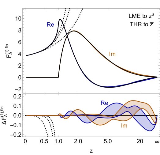
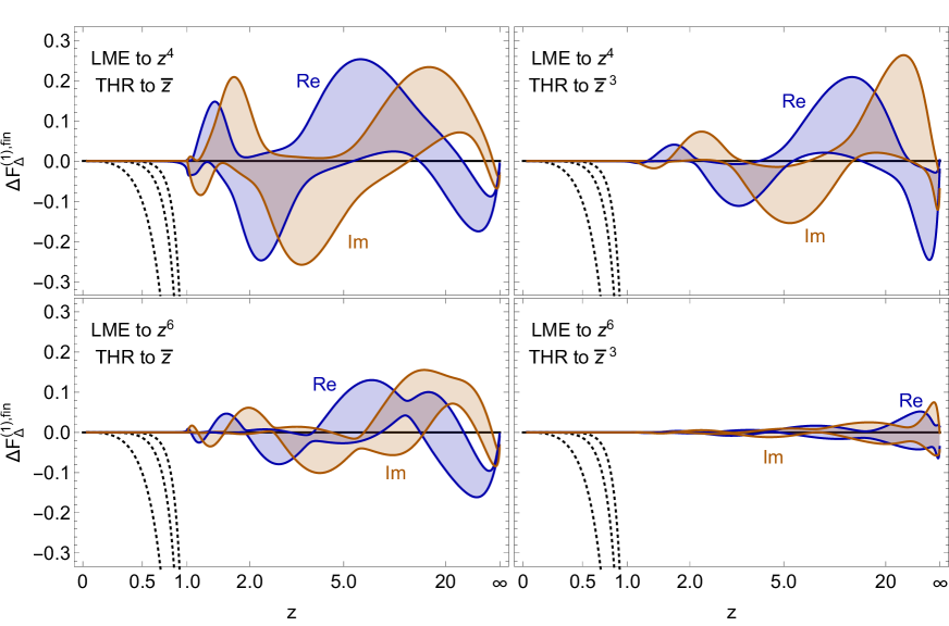
We show in Figure 2 that the exact result for the two-loop form factor can be reproduced very well with the same amount of information that is available at three loops. The shaded region is spanned by the standard deviation w.r.t. to the mean value of a set of 20 approximants for each considered set $\{n,m\}$. These approximants are available in the ancillary file [31]. Figure 3, where the difference between the exact result and the approximations is shown, demonstrates that the approximation can be systematically improved by including more expansion coefficients. We compare the results based on the input used in Figure 2 (lower left panel) to results where fewer expansion coefficients for large top quark masses are used (upper left panel). Furthermore, we also show results where additional information from threshold is incorporated in the construction of the Padé approximations (panels on the right).

Figure 4: Our approximations for the real and imaginary parts of the three-loop triangle form factor are shown in blue and orange, respectively. The bands give the standard deviation of the considered set of Padé approximants. The dashed lines correspond to the real part up to order $z^{2}$, $z^{4}$ and $z^{6}$. The lower panel shows the differences to the central values; see text for details.

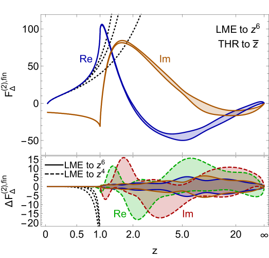
Our approximation of the three-loop form factor is shown in Figure 4 and represents the main result of this paper. At three loops the LME and threshold coefficients develop terms linear in $L_{s}=\log(-4z-i0)$. We construct separate Padé approximants for the coefficient such that we obtain an approximation of the form

$$F_{\triangle}^{(2),\rm fin}(z(\omega))\simeq\frac{[n/m]_{0}(\omega)+F_{\triangle}^{(2),\rm sub}}{1+a_{R,0}z(\omega)}+\frac{[k/l]_{1}(\omega)L_{s}}{1+a_{R,1}z(\omega)}\,,$$ (16)

where the subscripts indicate the power of $L_{s}$. Note that the Padé approximants of the $L_{s}$-independent and linear-$L_{s}$ term are averaged independently using separate values of $a_{R}$. The threshold subtraction (cf. Eq. (9)) is only needed for the first term in Eq. (16). The lower panel in Figure 4 shows the differences from the central values (obtained using seven expansion terms for small $z$) both with seven and five input terms from the large top quark mass expansion as solid and dashed boundaries of the uncertainty bands, respectively. One observes over the whole range in $z$ (except for a small region for $z\approx 10$) that the solid bands lie within the dashed band. Below threshold ($z=1$) our method results in tiny uncertainties for both the real and imaginary parts of the form factor. For $1\leq z\leq 2$ the form factor is numerically large and we thus observe small relative uncertainties. Although the absolute uncertainty becomes larger for higher values of $z$ we can provide a good approximation with an uncertainty which is sufficiently small for phenomenological applications.

Figure 5: Our approximations for the three-loop form factor separated according to the light-fermion contributions.

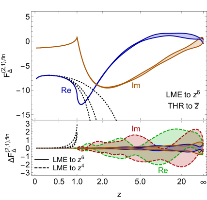
In order to facilitate the comparison with a future exact calculation we split our three-loop result according to the number of light fermions and write

$$F_{\triangle}^{(2),\rm fin}(z)=F_{\triangle}^{(2,0),\rm fin}(z)+n_{l}F_{\triangle}^{(2,1),\rm fin}(z)+n_{l}^{2}F_{\triangle}^{(2,2),\rm fin}(z)\,,$$ (17)

where $n_{l}=5$ is the number of light flavors. Note that $F_{\triangle}^{(2,0),\rm fin}(z)$ contains contributions with closed massive loops, which are numerically less important than the $n_{l}$ terms. There are no three-loop vertex diagrams which contain two closed fermion loops; $F_{\triangle}^{(2,2),\rm fin}(z)$ is completely determined by the infra-red subtraction terms. In fact, it is proportional to $F_{\triangle}^{(0)}$ and we will not discuss it further.

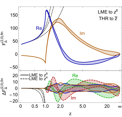
The results for $F_{\triangle}^{(2,0),\rm fin}(z)$ and $F_{\triangle}^{(2,1),\rm fin}(z)$ are shown in Figure 5, adopting the notation from Figure 4. Both coefficients show a convergence which is very similar to $F_{\triangle}^{(2),\rm fin}$. Summing up the coefficients leads to good agreement with the result (16) but with a larger uncertainty which is why (16) should be used for numerical applications. Note that the heavy-quark contribution to $F_{\triangle}^{(2),\rm fin}(z)$ is the only result where the exclusion criterion (14) has been used whereas for all other results (13) is applied.

Figure 6: The three-loop result for the form factor $F_{\triangle}^{(2),\rm fin}$ for space-like momenta. The dashed lines correspond to the real part of the LME approximation up to order $z^{2}$, $z^{3}$, $z^{4}$, $z^{5}$ and $z^{6}$. The same notation as in Figure 5 is adopted.

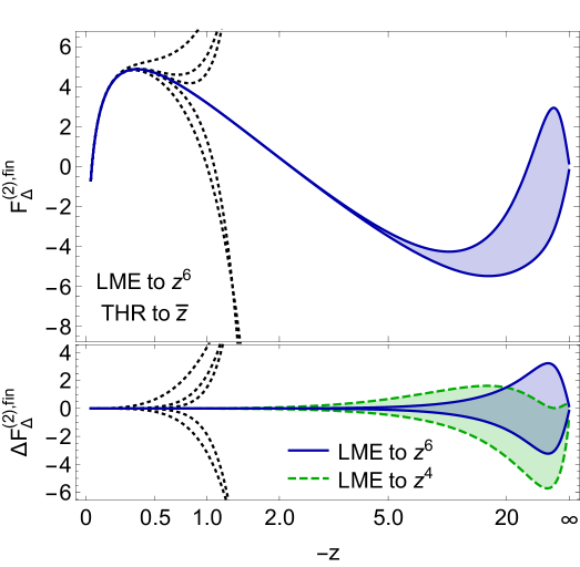
Finally, we present in Figure 6 results for the three-loop form factor for $z<0$. One observes small uncertainties for $|z|<5$ which become larger when $z$ becomes more negative. For $|z|>20$ the Padé approximation procedure does not lead to accurate results, we note that incorporating additional expansion terms does not significantly affect the size of the uncertainty. Note that the large top quark mass expansion shows an alternating behaviour.

Together with this paper we provide representative Padé approximants for all plots shown in this section in an ancillary file [31].

4 Conclusion

We compute three-loop corrections to the Higgs-gluon form factor including finite top quark mass effects. Our approach is based on the combination of analytic results from two kinematic regions: the expansion for large top quark mass and the top quark threshold. In addition, we incorporate the information that the form factors vanish at high energies by a rescaling (cf. Eq. (12)). For the rescaled form factors, we apply a conformal mapping and a subsequent Padé approximation. We first apply our method at two loops and show that we can reproduce the known results. The two-loop expression is also used to demonstrate that our estimate for the uncertainty works reliably. Our main result is shown in Figure 4 where we plot the three-loop form factor in the time-like momentum region. This plot can be reproduced using the approximation functions which are provided in the ancillary file [31]. We have shown that our results can be systematically improved by incorporating more expansion terms into the analysis.

References

- [1] D. de Florian et al. [LHC Higgs Cross Section Working Group], arXiv:1610.07922 [hep-ph].
- [2] M. Spira, A. Djouadi, D. Graudenz and P. M. Zerwas, Nucl. Phys. B 453 (1995) 17 [hep-ph/9504378].
- [3] R. V. Harlander and W. B. Kilgore, Phys. Rev. Lett. 88 (2002) 201801 [arXiv:hep-ph/0201206].
- [4] C. Anastasiou and K. Melnikov, Nucl. Phys. B 646 (2002) 220 [arXiv:hep-ph/0207004].
- [5] V. Ravindran, J. Smith and W. L. van Neerven, Nucl. Phys. B 665 (2003) 325 [arXiv:hep-ph/0302135].
- [6] R. V. Harlander and K. J. Ozeren, JHEP 0911 (2009) 088 [arXiv:0909.3420 [hep-ph]].
- [7] A. Pak, M. Rogal and M. Steinhauser, JHEP 1002 (2010) 025 [arXiv:0911.4662 [hep-ph]].
- [8] R. V. Harlander, H. Mantler, S. Marzani and K. J. Ozeren, Eur. Phys. J. C 66 (2010) 359 [arXiv:0912.2104 [hep-ph]].
- [9] A. Pak, M. Rogal and M. Steinhauser, JHEP 1109 (2011) 088 [arXiv:1107.3391 [hep-ph]].
- [10] C. Anastasiou, C. Duhr, F. Dulat, E. Furlan, T. Gehrmann, F. Herzog, A. Lazopoulos and B. Mistlberger, JHEP 1605 (2016) 058 [arXiv:1602.00695 [hep-ph]].
- [11] B. Mistlberger, JHEP 1805 (2018) 028 [arXiv:1802.00833 [hep-ph]].
- [12] F. Caola and K. Melnikov, Phys. Rev. D 88 (2013) 054024 [arXiv:1307.4935 [hep-ph]].
- [13] R. Harlander and P. Kant, JHEP 0512 (2005) 015 [hep-ph/0509189].
- [14] C. Anastasiou, S. Beerli, S. Bucherer, A. Daleo and Z. Kunszt, JHEP 0701 (2007) 082 [hep-ph/0611236].
- [15] U. Aglietti, R. Bonciani, G. Degrassi and A. Vicini, JHEP 0701 (2007) 021 [hep-ph/0611266].
- [16] R. V. Harlander and K. J. Ozeren, Phys. Lett. B 679 (2009) 467 [arXiv:0907.2997 [hep-ph]].
- [17] A. Pak, M. Rogal and M. Steinhauser, Phys. Lett. B 679 (2009) 473 [arXiv:0907.2998 [hep-ph]].
- [18] R. Gröber, A. Maier and T. Rauh, JHEP 1803 (2018) 020 [arXiv:1709.07799 [hep-ph]].
- [19] P. A. Baikov and D. J. Broadhurst, In Pisa 1995, New computing techniques in physics research 167-172 [hep-ph/9504398].
- [20] D. J. Broadhurst, J. Fleischer and O. V. Tarasov, Z. Phys. C 60 (1993) 287 [hep-ph/9304303].
- [21] J. Fleischer and O. V. Tarasov, Z. Phys. C 64 (1994) 413 [hep-ph/9403230].
- [22] K. G. Chetyrkin, J. H. Kühn and M. Steinhauser, Phys. Lett. B 371 (1996) 93 [hep-ph/9511430].
- [23] K. G. Chetyrkin, R. Harlander and M. Steinhauser, Phys. Rev. D 58 (1998) 014012 [hep-ph/9801432].
- [24] A. H. Hoang, V. Mateu and S. Mohammad Zebarjad, Nucl. Phys. B 813 (2009) 349 [arXiv:0807.4173 [hep-ph]].
- [25] Y. Kiyo, A. Maier, P. Maierhöfer and P. Marquard, Nucl. Phys. B 823 (2009) 269 [arXiv:0907.2120 [hep-ph]].
- [26] A. Maier and P. Marquard, Phys. Rev. D 97 (2018) no.5, 056016 [arXiv:1710.03724 [hep-ph]].
- [27] S. Catani, Phys. Lett. B 427 (1998) 161 [hep-ph/9802439].
- [28] D. de Florian and J. Mazzitelli, JHEP 1212 (2012) 088 [arXiv:1209.0673 [hep-ph]].
- [29] J. Davies and M. Steinhauser, “Three-loop form factors for Higgs boson pair production in the large top mass limit”, in preparation.
- [30] M. Beneke, J. Piclum and T. Rauh, Nucl. Phys. B 880 (2014) 414 [arXiv:1312.4792 [hep-ph]].
-
[31]
https://www.ttp.kit.edu/preprints/2019/ttp19-014/.