Limiting fragmentation as an initial-state probe in heavy ion collisions

Abstract

We discuss limiting fragmentation within a few currently popular phenomenological models. We show that popular Glauber-inspired models of particle production in heavy ion collisions, such as the two-component model, generally fail to reproduce limiting fragmentation when all energies and system sizes experimentally available are considered. This is due to the energy-dependence of number of participants and number of collisions. We quantify this violation in terms of the model parameters. We also make the same calculation within a Color Glass Condensate scenario and show that the dependence of the saturation scale on the number of participants generally leads to violation of limiting fragmentation. We further argue that wounded parton models, provided the nucleon size and parton density vary predominantly with Bjorken $x$, could in principle reproduce both multiplicity dependence with energy and limiting fragmentation. We suggest, therefore, that an experimental measurement of deviation from limiting fragmentation in heavy ion collisions, for different system sizes and including the experimentally available range of energies, is a powerful test of initial state models.

I Introduction

The phenomenon of limiting fragmentation in hadronic collisions was originally both experimentally seen busza1 ; busza2 and theoretically explained at the origins of the QCD theory of strong interactions yen .

The definition of limiting fragmentation is that

$$\left.\frac{d^{2}N}{d\kappa^{2}}\right|_{\kappa=y-y_{0}}=C\phantom{A},\phantom{A}\frac{\sqrt{s}}{C}\frac{dC}{d\sqrt{s}}\ll 1\phantom{A},\phantom{A}y_{0}=\ln\frac{\sqrt{s}}{m_{p}}$$ (1)

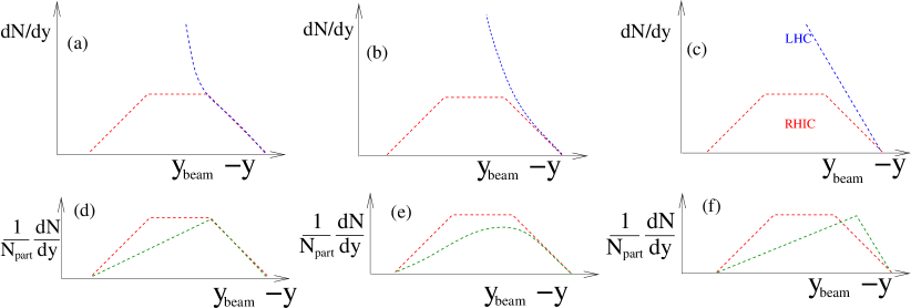
Where $C\simeq 0.65$ is an energy-independent constant and $m_{p}$ the proton mass. A qualitative illustration of limiting fragmentation is shown on the panel (a) of Fig. 1. As it happens well-away from mid-rapidity, both distributions in rapidity $y$ and pseudo-rapidity $\eta$ can be used for limiting fragmentation (In fact the experimental data discussed later was collected in pseudo-rapidity. See the appendix on a discussion of this issue).

When plotted against $y-y_{0}$ (the difference between rapidity and beam rapidity), multiplicity distributions away from mid-rapidity should fall on a universal curve, independent of center of mass energy. Using the second derivative of the rapidity distribution, as defined in Eq. 1, provides a dimensionless quantitative estimator which should vanish within error bar if limiting fragmentation holds, be $\gg 1$ if it breaks down, and is relatively insensitive to rapidity/pseudorapidity differences (see appendix). Using directly $C$ of Eq. 1 allows for a nice graphic comparison, while the logarithmic derivative $\frac{dC}{d\ln\sqrt{s}}$ of makes large fluctuations blow up, but allows a quantitative comparison across different energy regimes.

The basic explanation for limiting fragmentation is to see it as a consequence of the parton model and Bjorken scaling halzen . The distribution functions of parton g, i.e. the parton amplitudes in the infinite momentum frame of the nucleon, depend on the nucleon momentum in a very particular way

$$\left|<N(p)|g(q)>\right|^{2}_{p\gg m_{N}}\sim f(x,\ln Q^{2})\phantom{A},\phantom{A}x=q/p$$ (2)

where $x$ is the momentum fraction and $Q^{2}$ the renormalization group momentum scale, corresponding to the momentum transfer of the process measuring $f(x,Q^{2})$.

Figure 1: (color online) Possible limiting fragmentation scenarios when LHC and lower energies are compared (top row) and an extended comparison with different system sizes (panels d,e,f). Case (a,d) presupposed an extended limiting fragmentation scenario up to the mid-rapidity plateau. Case (b,e) is a smooth breaking of scaling interpolating between a universal fragmentation regime and the central rapidity plateau, case (c,f) is wholesale violation, both at central rapidity and in the fragmentation region. The bottom row panels d,e,f show the three cases when a symmetric AA collision is compared to an asymmetric pA or dA collision.

As the parton mass is negligible its momentum rapidity $y_{g}$ is related to $x$ very simply, as

$$y_{g}=\pm\ln\left(1/x\right)$$ (3)

Because of asymptotic freedom, the dependence on $Q^{2}$ as well as any hadronization effects do not change the final momentum much. As a result, away from mid-rapidity fragmentation does not change the rapidity of the hadron with respect to the parton. Thus, if one assumes parton interactions are local in rapidity, and the resulting hadron is not shifted in rapidity with respect to the parton, in other words (the delta function is simply the momentum conservation in the longitudinal axis)

$$\frac{dN}{dy}\sim\int dx_{A}dx_{B}f(x_{A})f(x_{B})\mathcal{N}(x_{A}\sqrt{s}/2,x_{B}\sqrt{s}/2)\times$$ (4)

$$\ \delta\left(\sinh\ln(1/x_{A})+\sinh\ln(1/x_{B})-\sinh y\right)$$

limiting fragmentation follows naturally, since asymptotic freedom and the longitudinal momentum conservation ensure that when $x_{A}\gg x_{B}$, corresponding to $y$ very different from zero, a universal curve for $dN/dy$ depending only on $x_{A}\simeq e^{y}$ emerges.

This reasoning is appropriate if the only dimensionful scale relevant to hadronic scattering is the nucleon size, i.e. if only one type of collisions, in a not-too varied range of energies is considered. Since then it has however been seen in a wide range of hadronic phobos ; phobosprl ; phobosrev ; whitebrahms and even nuclear jeon collisions. Indeed, a variety of approaches, ranging from Landau hydrodynamics steinberg to the Color Glass Condensate busza ; jamal ; stasto ; andre1 ; andre2 to phenomenological transport models such as “AMPT” ampt0 (whose limiting fragmentation is investigated in ampt ), string percolation capella ; palh1 ; palh2 and relativistic diffusion wols are at least roughly compatible with it.

However, limiting fragmentation turned out to work for a wider spectrum of energies, rapidities and system sizes than initially suspected. At Relativistic Heavy Ion Collider (RHIC) energies (5-200 GeV), it seems to hold busza ; phobos ; jeon for all system sizes and all energies up to an energy-dependent rapidity interval of $\mathcal{O}\left(1\right)$ or so. This can be surprising. Close to mid-rapidity, at the highest energy density, a lot of additional effects, from high energy fragmenting jets to soft gluon effects to viscous entropy production, are expected to contribute particles in a way that evolves non-trivially with energy. The reason why energy-specific dynamics should converge to a universal distribution away from mid-rapidity is not immediately clear, since Bjorken scaling means remnants of these processes should be present away from mid-rapidity.

At RHIC energies, there was no problem to incorporate this extended limiting fragmentation into phenomenological models capella , if not theories. A qualitative explanation links weakly ; surprises limiting fragmentation to the close-to-logarithmic energy-dependence of multiplicity $dN/dy$ per participant $N_{part}$ at mid-rapidity. The logarithmic dependence of the rapidity width (the base of the distribution) is fixed by kinematics. Then, “extra parton sources” at mid rapidity weakly ; capella produce strings connected to rapidity edges, ensuring the self-similarity of the total multiplicity distribution.

The Large Hadron Collider (LHC) seems to have added some new twists to this story when energies of several TeV were reached. It has conclusively deviated from logarithmic scaling of multiplicity w.r.t. energy (see for example alice ), at the same time convincingly breaking the pure number of participants scaling glabrev ; glauber of particle production. This has motivated the development of more complicated characterizations of the Glauber initial state, generally based on “multi-component scenarios”. For instance, core-corona models posit that the event is characterized both by a “soft medium” (participants that underwent multiple collisions) as well as a few hard collisions (a “corona” of singe-hit participants). More phenomenologically alice ; fernando ; corecorona one could assume wounded nucleons and collisions provide different admixtures to the multiplicity.

In view of these “new developments”, it is worth revisiting limiting fragmentation at this energy. It should first be noted that it has not as yet been confirmed or falsified experimentally alicey ; cmsy ; atlasy , partially because LHC experiments have not as yet explored rapidity regimes high enough to be compared even with RHIC energies. In principle, the three possible scenarios are described in the panels of Fig. 1. One can continue to have perfect limiting fragmentation in the whole region away from mid-rapidity (panel(a) ), limiting fragmentation can smoothly be achieved as rapidity increases (panel (b)) or it can just totally break down (panel (c)). The bottom panels d,e,f show the corresponding possible scenarios in pA collisions once the distribution is normalized by the number of participants (note that only one side can limiting fragment since pA is rapidity asymmetric).

In this work, we argue that such an investigation is indeed necessary. We show that the most-commonly used model for the initial state of heavy ion collisions, the Glauber model, will generally break limiting fragmentation in the parameter space where it fits LHC data provided all energies and system sizes are considered. We show that the same is true for Color Glass Condensate (CGC) models, as implemented in andre1 ; andre2 .

We then argue that a currently popular model capable of bringing the applicability of limiting fragmentation to LHC energies and varying system sizes, provided it is indeed confirmed experimentally, is a “wounded parton model”, with Glauber wounded partons woundq1 ; woundq2 ; woundq3 ; woundq4 ; woundq5 smeared in rapidity space according to Bjorken scaling. We conclude with some experimental considerations regarding this observable.

II Limiting fragmentation and the Glauber model

The two component model is a physically intuitive parametrization of multiplicity glauber ; glabrev . The basic idea is that, in a nucleus-nucleus collision some particles are produced in hard scatterings as a result of fragmentation of parton-parton interactions. The rest of the particles, typically the majority, arise from “wounded nucleons”, nuclei that underwent a collision, emitted color charge, and then emitted particles due to non-perturbative color neutralization. An alternative but related picture is the “core-corona” model, where wounded nucleons form “the medium” (presumably a quark-gluon plasma), while individual nucleon-nucleon collisions (and nuclei which underwent just one collision) can be thought of as being similar to proton-proton collisions corecorona .

Thus, quantitatively, the two sources of particles are related by the parameter $f$, controlling the input of the number of collisions $N_{coll}$ vs. number of participants $N_{part}$ to the total number of “ancestor particle sources” $N_{anc}$:

$$N_{anc}=fN_{part}+(1-f)N_{coll}\,.$$ (5)

Physically, $N_{coll}$ scaling reflects the fragmentation of partons produced in a QCD collision. $N_{part}$ reflects the products “wounded nucleons” which emit partons as they color-neutralize.

To describe multiplicity we need another parameter $\alpha$, controlling how many particles are produced per ancestor, interpolating between logarithmic ($\alpha=0$) and power-law ($\alpha>0$) limits

$$\left.\frac{dN}{dy}\right|_{y=0}=\mathcal{N}_{0}N_{anc}\int_{1}^{\sqrt{s}}\zeta^{\alpha-1}d\zeta$$ (6)

where $\mathcal{N}_{0}$ is an overall normalization parameter, uncorrelated with $f,\alpha$.

In fernando and preceding literature, it was assumed that $\alpha$ is the same for $pp$, $pA$ and $AA$ collisions. This means one knows $\alpha$ from $pp$ fits and can obtain $f$ from $AA$ fits. In other words, The different exponents seen experimentally in these systems are due entirely from the fluctuation of $N_{part}$ and $N_{coll}$ of a two-component model.

This, while possible, is not guaranteed. It is well known (The “EMC effect”) from $eA$ scattering that parton distribution functions significantly change in a nuclear medium emc . Given that different energy regimes probe different $x$, it is plausible that the difference between proton and nuclear medium could give rise of different excitation functions of $dN/dy$ on top of geometric effects. This, however, means that the $f$ parameter and the $\alpha$ parameter need to be understood together within a fit to experimental data, since the Hessian matrix relating them will contain a diagonal term.

A phenomenology tool comes from the fact that the cross-sectional area depends on energy, with its dependence roughly

$$\sigma=A_{1}\ln\left(\frac{\sqrt{s}}{m_{p}}\right)+A_{2}\left(\ln\left(\frac{\sqrt{s}}{m_{p}}\right)\right)^{2}$$ (7)

with $A_{1}=25$ and $A_{2}=0.146$ fitted from data such as sigma

It then becomes clear that in a general Glauber model, the ratio of $N_{coll}/N_{part}$ will depend on energy as well.

Figure 2: (color online) Panel (a): The distribution of $N_{part}$ as a function of energy. Panel (b): The subsequent evolution of $N_{coll}/N_{part}$ in a Glauber model, with the best fit to the most central collisions added as a line

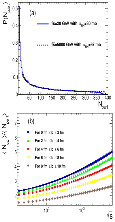
Indeed, a calculation using the model described in phobos ; fernando is shown in Fig. 2. While the number of participants varies very little with energy (as is obvious, since only variations in higher order moments are permitted by definition), the number of collisions varies systematically with the increase of the inelastic scattering cross-section.

The best fit, also shown in the figure, can be parameterized by

$$N_{cp}(\sqrt{s})=T\left(\ln\left(\frac{\sqrt{s}}{m_{p}}\right)\right)^{2}+G\ln\left(\frac{\sqrt{s}}{m_{p}}\right)+J,$$ (8)

Where $T,G,J$ are fit parameters (See footnote 1. The $\chi^{2}$ here is negligible, $\sim 10^{-5}$). For the top centrality bin of Au-Au, used later in multiplicity fits, their numerical values are $T=0.043$, $G=-0.045$ e $J=2.1$

While, as panel (a) shows, the event by event $N_{part}$ distribution is relatively constant in energy (unsurprisingly, since it is bounded between zero and 2A globally, and to a good approximation to the local transverse density at each point in the transverse area), the ratio of $N_{coll}/N_{part}$ has a monotonic increase. It is intuitively clear that in a general two-component model this will introduce an energy dependence on $dN/dy$ which does not appear in rapidity, since both $N_{part}$ and $N_{coll}$ are parameters characterizing the whole event, rapidity independent.

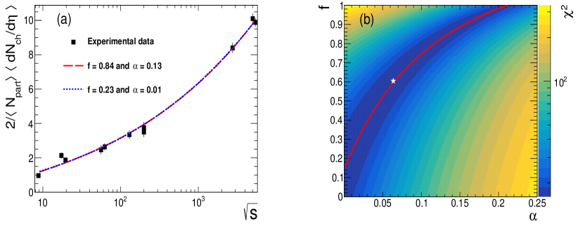
It is clear that $\alpha$ and $f$ are strongly correlated by experimental data. We therefore made a $\chi^{2}$ contour using the data of alice to fit them. The results are shown in Fig. 3, panel (b). We highlight the curve going through the major axis of the ellipse in $f-\alpha$ space, parametrizeable by

$$f_{fit}(\alpha)=F_{1}\alpha^{4}+F_{2}\alpha^{3}+F_{3}\alpha^{2}+F_{4}\alpha+F_{5},$$ (9)

where the fitted values are $F_{1...5}=-250.1,175.8,-53.6,9.9,0.14$ (See footnote 1. $\chi^{2}\sim 10^{-2}$).

The $\mathcal{N}_{0}$ parameter of course is also correlated with $f,\alpha$. In terms of $\alpha$ its minimum can be parametrized as

$$\mathcal{N}_{0}\simeq N_{1}\alpha^{2}+N_{2}\alpha+N_{3}$$ (10)

where $N_{1..3}=-3.35,1.32,0.27$ (See footnote 1. The $\chi^{2}\sim 10^{-3}$).

We also note that the inclusion of both in a simultaneous fit greatly widens the space of $f-\alpha$ allowed, and in fact the fit seems to prefer a value of $f$ considerably lower ($N_{coll}$ dominated ancestors) than most of the work of this kind.

Panel (a), showing the fit quality of the opposite ends compared to experimental data, however, demonstrates one must not take this too seriously (although it can also give a decent fit of eccentricities, see for instance urom ) since the correlation between the fit parameters (as well as the overall normalization) is such that the two extremes do a very similar job of fitting the data and in fact generate a nearly identical curve. This, and the disagreements at lower energy also make the $\chi^{2}$ contour deviate significantly from the Gaussian.

Given these ambiguities, our strategy, rather than focusing on inferring a tighter bound on $f-\alpha$ space, is to use this fit to define a relation between the two variables, based on $f_{fit}(\alpha)$, that fixes the mid-rapidity curve, and investigate limiting fragmentation given this relation.

Figure 3: (color online) Panel (a): experimental data, referenced in alice with the opposite ends of the fitted curve. Panel (b): Contour of fit to midrapidity experimental data in $\alpha-f$, with best fit line highlighted and a star denoting the $\chi^{2}$ minimum.

We therefore use the graph where Eq. 9 was used to parametrize $f_{fit}(\alpha)$ we now scan through $\alpha$ to check how limiting fragmentation behaves for the class of Glauber models fitting mid-rapidity.

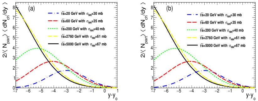
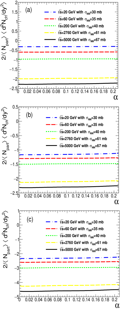
First, we use the opposite ends of $(f,\alpha)$ parameter space to investigate the behavior away from mid-rapidity of $dN/dy$, assuming Gaussian distributions in a manner similar to ampt , with widths given kinematically and heights by the observed mid-rapidity. As can be seen in Fig 4, at both extremes limiting fragmentation is broken by a similar manner.

Figure 4: (color online) Gaussian rapidity dependencies with the width given by a Landau-like kinematic parametrization, and the height extrapolated from pairs of parameters $f,\alpha$ adjusted to reproduce data at mid-rapidity

To quantify this violation further, we used a Gaussian, a trapezoidal and a triangular distribution in $\eta$, with the bottom base given by kinematics $\Delta\eta_{bottom}=\ln(\sqrt{s}/m_{p})$ , while the top base as universally a fraction either $\Delta\eta_{top}=0$ (for a triangle and a Gaussian) or $\Delta\eta_{top}=\Delta\eta_{bottom}/2$ of the bottom base (for a trapezium). The height is chosen by the two-component model calculation.

The results are shown in Fig. 5. As can be seen, all cases exhibit practically constant and sizable violations of limiting fragmentation for all values of $(f,\alpha)$. The constancy is not a surprise, given the good fit of the central rapidity for all values of $\alpha,f_{fit}(\alpha)$ Furthermore, the quantitative amount for the violation of limiting fragmentation is to a good extent independent of both the value of $\alpha$ and the model used. We can therefore conclude with some confidence this violation is approximately what can be expected in any distribution respecting mid-rapidity multiplicity and kinematic constraints.

Figure 5: (color online) The gradient of the rapidity distribution at $y-y_{0}=3$ assuming a Gaussian (Panel (a)), triangular (Panel (b)) and trapezoidal (Panel (c)) shapes respectively, against the $\alpha$ parameter, with the corresponding $f=f_{fit}(\alpha)$ parameter adjusted to reproduce data at mid-rapidity (Fig. 3).

Note that, while very simple, these distributions have the same functional form as the pseudorapidity distributions measured in alicey . The triangular distribution also has the advantage to generate limiting fragmentation analytically at $\alpha\rightarrow 0,f\rightarrow 1$, while the Gaussian one reproduces it to a good approximation for $\alpha=1/4,f=1$ steinberg .

This limit which is not captured in our plot, since it is very far from the best fit line: $f\rightarrow 1$ prefers higher numbers of $\alpha$, which breaks limiting fragmentation. $\alpha\rightarrow 0$ prefers very low $f$ (collision-dominated multiplicity) which again breaks limiting fragmentation. We can therefore make the qualitative statement that a general Glauber model cannot realistically fit mid-rapidity multiplicity without a significant break in limiting fragmentation. This is experimentally testable.

It is very simple to understand the universality of the violation of the limiting fragmentation, and generalize from Gaussians and Trapeziums (where one can get a quantitative analytically calculable answer) w.r.t. any rapidity shape, where the difference should be within a factor $\mathcal{O}\left(1\right)$ of the one calculated here.

All we need to assume, both are crucial assumptions for the Glauber model of particle production as described here, is

(i)

An emission function $F(y)$ which is specific to each ancestor. Different emission functions $F_{part}(y)$ and $F_{coll}(y)$ would not change the result

$$\frac{dN}{dy}=\sum_{N_{anc}}F(y)\sim N_{part}F_{part}(y)+N_{coll}F_{coll}(y)$$ (11)

(ii)

The base of the emission function is kinematically determined to be $\sim\ln\left(\frac{\sqrt{s}}{m_{p}}\right)$

This section makes it clear that, as long as $N_{coll}/N_{part}$ evolves non-logarithmically and $f\neq 0$ (as is mandated by experimental data), $N_{part}^{-1}d^{2}N/d\eta^{2}$ cannot be universal. These statements will hold as long as assumptions (i) and (ii) are correct, and putting in reasonable distributions shows violations big enough to be qualitative rather than small corrections. In particular, the middle scenario in Fig. 1 (smooth approach to limiting fragmentation) is excluded by assumption (i) and by the inability of $f=1$ models to fit midrapidity data, since for this to happen the rapidity distributions of individual ancestors must be aware at how the number of ancestors (producing the mid-rapidity peak) increases.

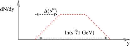
Let us illustrate this by extending our analytically solvable model: We take the trapezium distribution (Fig. 5 panel (b)) but impose an arbitrary variation with $\sqrt{s}$ of the top rapidity plateau $\Delta(\sqrt{s})$ (Since this variation is arbitrary, this includes the case of $N_{part}$ and $N_{coll}$ having different plateaus (Fig. 6).

Figure 6: A trapezoidal rapidity distribution with a varying width parameter

Calling $N_{cp}(\sqrt{s})$ is the ratio of participants to collisions (shown in Fig. 2 and Eq 8 ), we will have

$$\left.\frac{d^{2}N}{dy^{2}}\right|_{\left|y-y_{0}\right|\ll y_{0}}=\frac{Z_{1}}{Z_{2}}$$ (12)

$$\ Z_{1}=-4\mathcal{N}_{0}N_{part}\left(f+(1-f)N_{cp}\left(\sqrt{s}\right)\right)\left(\sqrt{s}^{\alpha}-1\right)$$

$$\ Z_{2}=\alpha\left(1-\Delta\left(\sqrt{s}\right)\right)\ln\left(\frac{\sqrt{s}}{m_{p}}\right)$$

Since the only things that are permitted to vary with energy are $N_{cp}$ and $\Delta$, this means that for limiting fragmentation to occur we must have

$$F_{1}\left(f,\alpha,N_{cp}\left(\sqrt{s}\right)\right)=CF_{2}\left(\Delta\left(\sqrt{s}\right)\right)$$ (13)

where $C$ is the constant defined in equation 1 and

$$F_{1}\left(f,\alpha,\sqrt{s}\right)=\frac{\mathcal{N}_{0}N_{part}}{\alpha}\times$$ (14)

$$\ \times\left(f+\left(1-f\right)N_{cp}\left(\sqrt{s}\right)\right)(\sqrt{s}^{\alpha}-1)$$

$$F_{2}\left(\Delta\left(\sqrt{s}\right)\right)=-\frac{1}{4}\left(1-\Delta\left(\sqrt{s}\right)\right)\ln\left(\frac{\sqrt{s}}{m_{p}}\right)$$ (15)

This is physically impossible. Not only because the first function depends on nuclear geometry and the cross-section area and the second just on the partonic structure, but because the first depends on $\alpha$ and the second does not.

For instance, let us suppose that the $\Delta$ evolution arises from particle distributions produced in $N_{part}$ and $N_{coll}$ having different widths (i.e. the fragmentation region is different for wounded nuclei than for parton-parton collisions, a wholly reasonable scenario), parametrized as $\Delta_{1,2}\ln\left(\frac{\sqrt{s}}{m_{p}}\right)$ where $\Delta_{1,2}$ are fixed coefficients.

This would mean

$$\Delta(\sqrt{s})=\frac{\mathcal{N}_{0}N_{part}\left(\sqrt{s}^{\alpha}-1\right)}{\alpha}\times$$ (16)

$$\ \times\left(\frac{f}{\Delta_{1}}+\frac{(1-f)}{\Delta_{2}}N_{cp}(\sqrt{s})\right)$$

this will lead to the supposed “constant“ $C$ of the form

$$C=\frac{-4\mathcal{N}_{0}N_{part}\left(\sqrt{s}^{\alpha}-1\right)}{\alpha\ln\left(\frac{\sqrt{s}}{m_{p}}\right)}\times$$ (17)

$$\ \times\frac{\left(f+\left(1-f\right)N_{cp}\left(\sqrt{s}\right)\right)}{\left(1-\left(\frac{\mathcal{N}_{0}N_{part}\left(\sqrt{s}^{\alpha}-1\right)}{\alpha}\right)W\left(\Delta_{1},\Delta_{2},f,\sqrt{s}\right)\right)}$$

where

$$\ W\left(\Delta_{1},\Delta_{2},f,\sqrt{s},\right)=\frac{f}{\Delta_{1}}+\frac{\left(1-f\right)}{\Delta_{2}}N_{cp}\left(\sqrt{s}\right)$$

A plot of $\sqrt{s}C^{-1}dC/d\sqrt{s}$, for $f=f_{fit}(\alpha)$ and $\alpha$ adjusted according to Fig. 3, $\mathcal{N}_{0}$ given by the correlated values Eq. 10 and $\Delta_{1,2}$ scaled by $\ln\left(\frac{\sqrt{s}}{m_{p}}\right)$ is shown in Fig. 7. It confirms the universality of breaking of limiting fragmentation within the Glauber model, by showing that any reasonable value of $\Delta_{1,2}$ does not satisfy Eq. 13 for an $f,\alpha$ given by the best fig parametrization Eq. 9.

Figure 7: (color online) A scan of the expected limiting fragmentation violation in conformal units, $\sqrt{s}C^{-1}dC/d\sqrt{s}$ as a function of the best fit parameters in rapidity data $\alpha,f_{fit}(\alpha)$ (kept fixed) as well as $\Delta_{1,2}$ (on the axes) the widths of $N_{part}$ and $N_{coll}$. The derivative was taken at $\sqrt{s}=$200 GeV. The three panels show the choices of $f,\alpha$ corresponding to the extremes of Fig. 3 (panel (a) and (c)) and the $\chi^{2}$ minimum (panel (b)). We verified that intermediate values are well described by a smooth interpolation between these two

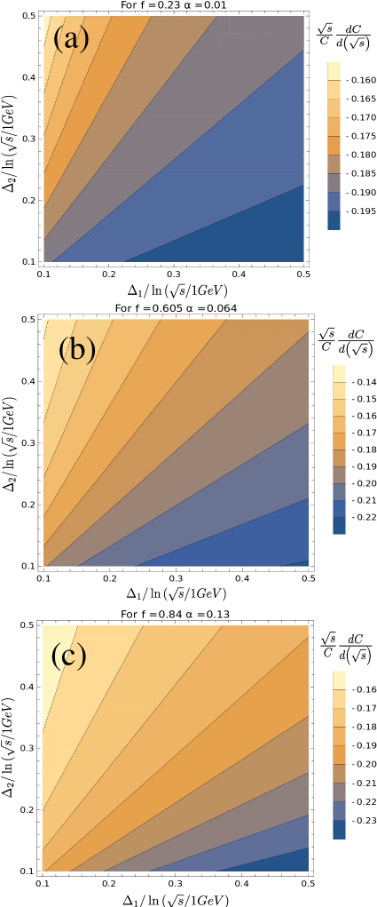
It is easy to see that similar equivalency, albeit with additional rapidity dependence, will arise for a Gaussian and any other shape. A comparison between $pA$ and $AA$ for the same number of participants (as in Fig. 1) would be even more problematic since for $pA$ $N_{coll}\simeq N_{part}-1$ while for $AA$ no such constraint is present.

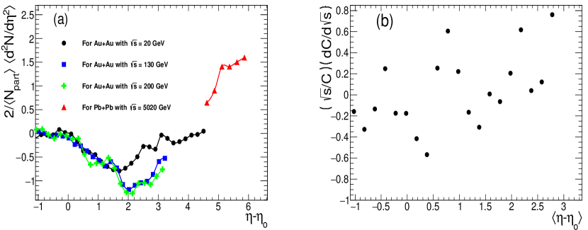
We also show (Fig. 8) a compedium of estimates of $d^{2}N/d^{2}\eta$ and the observable seen in Fig. 7, obtained with numerical derivatives of experimental data compiled in jeon from phobosprl and for energies of 130 and 200 GeV (where $dN/dy$ per participant is still approximately logarithmic with $\sqrt{s}$). Panel (a) of the graph appears to show, by eye, that limiting fragmentation is broken only weakly, if at all. Panel (b), where a common normalization with theory was included, shows a breaking comparable to Fig. 7 in magnitude, but, unlike Fig. 7, spread around zero.

This figure is included as a proof-of-concept, but extreme care should be taken to interpret it as a quantitative limit. The data it is based on does not include error bars (jeon and references ), and the multiplication by $\sqrt{s}$, necessary to define a dimensionless observable quantifying breaking, magnifies fluctuations invisible to the naked eye in Fig. 8’s panel (a). The fact that the points oscillate chaotically around zero strongly suggest that Fig. 8’s panel (b) is in fact dominated by statistical fluctuations, and quantitatively the violation of limiting fragmentation until the top RHIC energies is parametrically smaller than that of Fig. 7. A reanalysis such as that of Fig. 8 by the members of the experimental collaborations, with access to raw data, and together with LHC data could potentially verify this claim.

Additionally, as was already noted in jeon , extrapolating to LHC energies (Fig. 8,10 of that work) means that any quantitative disagreement with limiting fragmentation seen at RHIC would be amplified by the departure from the logarithmic energy dependence per participant at LHC energies (predicted by a number of models in jeon and confirmed). A logarithmic derivative, such as the one we defined ($\sqrt{s}d/d\sqrt{s}=d/d\ln\sqrt{s}$), allows to highlight the quantitative violation of limiting fragmentation inherent in this effect despite the large energy gap between top RHIC and bottom LHC energies.

Given these considerations, Fig. 7 and Fig. 8 strongly motivate a precise quantitative estimate of the violation of limiting fragmentation both across LHC and RHIC energy regimes.

Figure 8: (color online) Panel (a): $d^{2}N/d\eta^{2}$ and the observable in Fig. 7 obtained from experimental data, from the compilation in jeon (data from phobosprl ) and alicey . Panel (b) shows the numerical derivative calculated between 130 and 200 GeV.

The persistence of limiting fragmentation, especially in the LHC energy regime, would preclude the system to be a superposition of nucleon-nucleon collisions. However, such a picture was called into doubt in the literature by models where partonic degrees of freedom appear at the nuclear level, such as the Color Glass and the wounded quark model. In the next section we describe what such models imply for limiting fragmentation.

III Partonic nuclear dynamics and limiting fragmentation

It is obvious from the discussion in the previous section that any $N_{coll}$ dependence on multiplicity is inherently incompatible with limiting fragmentation. Ultimately, the last section can be summarized in a simple statement: It is an experimental fact that the cross-sectional area changes with energy, and this by itself will introduce an energy-dependent contribution which, unless unnecessary fine-tuning is introduced, will never seep into rapidity dependence.

All Glauber model analyses so far, however, show that some $N_{coll}$ dependence is unavoidable if nucleon-nucleon collisions are extrapolated from $pp$ to $AA$. One answer to this is the “wounded quark model” woundq1 ; woundq2 ; woundq3 ; woundq4 ; woundq5 (more accurately described as wounded parton model), which also could be justified from a dynamics such as that of bgk .

It is unsurprising that wounded parton models have more leeway in fitting multiplicities with only participant scaling, since they by definition have a greater number of parameters: Very little is known about configuration space parton distribution of the nucleons (the “three constituent quarks” picture is an obvious simplification at high energies). Thus, one can substitute the effect of varying $f,\alpha$ in the two component model with parameters describing the parton transverse and longitudinal distribution within the nucleon. The works cited above, in their own way, essentially accomplished this.

One can however also note that the fundamental difference here is that the “size of the nucleon”, i.e. the Fourier transform of the nucleon form factor, is something that is allowed to vary with Bjorken $x$. Boost-invariance, built into the parton model, means that space-time rapidity of the parton’s trajectory and momentum rapidity are equal

$$y=-\ln\left(x^{-1}\right)=\frac{1}{2}\ln\left(\frac{z+t}{z-t}\right)$$ (18)

As fig 9 shows, one can imagine a nucleon nucleon collision within such a model as a superposition of a “train” of collisions, of transverse shapes located in different bins in Bjorken $x$.

Each participant starts from that Bjorken $x$, is shifted by one or more collisions to a different Bjorken $x$, and finally emits hadrons according to some distribution in rapidity determined by this final Bjorken $x$ and fragmentation dynamics. The transverse nucleon shape at each $x$ can also vary, and hence can mimic the variation of the “nucleon-nucleon cross-section” with energy via the growth of the typical $x$ with $\sqrt{s}$. Crucially, the same variation will occur in rapidity.

Figure 9: An illustration of the Glauber model based on wounded nucleons vs wounded partons. The latter has the distinction that each initial degree of freedom is at a different Bjorken $x$, and shifts to a different $x$ (i.e. final rapidity bin) once ”wounded”

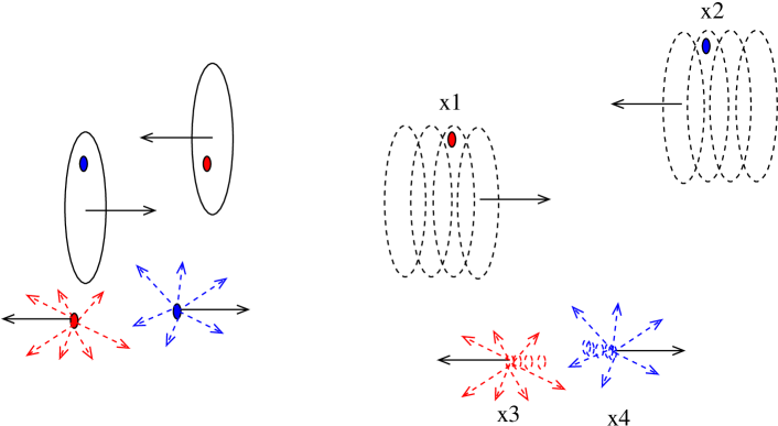
We investigate this idea with a toy model, combining a Glauber-type wounded parton model with a transverse quark size parameterized by $Q_{s}(x)$. Note that “s” in $Q_{s}$ here might stand for “size”, not for saturation, i.e. it might represent a nucleon-specific rather than transverse space-specific scale. All that we need is that $Q_{s}$ is allowed to vary with Bjorken $x$. Basically, we assume “a tube of pancakes”, each at a momentum and spacetime rapidity $e^{\pm x}$ of transverse size $Q_{s}(x)^{-1}$.

Let us briefly recap as to how this setup generates limiting fragmentation. The key assumptions relating limiting fragmentation to the parton model are:

(a)

All transverse momentum scale (denoted here by $k$) dependence is via $(k/Q_{s}(x))^{2}$, a scale (reflecting saturation or size) depending only on $x$, usually $\sim x^{-\lambda}$.

(b)

Normalization of $\tilde{T}(k,x)$ depends only on $x$ (possibly via $Q_{s}(x)$) or be constant

$$\ \int^{Q^{2}}\frac{d^{2}p_{T}}{p_{T}^{2}}\tilde{T}(p_{T},x)\sim\mathcal{N}(x)$$

(c)

Asymptotic freedom. Most partons are produced with little shifts in momenta. As a result, if $-\ln x$ is not $\gg 1$, one can assume $x\sim e^{-y}$ of the produced parton. In simple language, asymptotic freedom prevents partons away from mid-rapidity to fragment away from their rapidity bin

Let us illustrate how these assumptions generically give limiting fragmentation in pp collisions. Extending the Glauber model formalism to such a system is simple

$$T_{A}(\mathbf{s})=\int\rho_{A}(\mathbf{s},z_{A})dz_{A}\rightarrow T_{A}(\mathbf{s},x)\sim F(x,Q_{s}(x))$$ (19)

With $Q_{s}(x)$ characterizing the nucleon size at that $x$.

Now the usual definition for $T_{AB}$ can be duly updated to

$$T_{AB}(\mathbf{\hat{b}},y)=\int T_{A}(\mathbf{s},x_{A})T_{B}(\mathbf{s}-\mathbf{\hat{b}},x_{B})\times$$ (20)

$$\ \times\delta\left(x_{A}+x_{B}-e^{-y}\right)d^{2}s$$

If one uses the standard formula for the number of collisions

$$\left\langle N_{coll}\left(\mathbf{\hat{b}}\right)\right\rangle=ABT_{AB}(\mathbf{\hat{b}})\sigma_{inel}^{qq}\text{,}$$ (21)

with Bjorken scaling and a conformal cross-section

$$\sigma_{inel}^{qq}=\frac{1}{p_{T}^{2}}\phantom{A},\phantom{A}x_{A,B}=\frac{p_{T}e^{\pm y}}{\sqrt{s}}$$ (22)

parallels, the $k_{T}$ factorization formula (derived through somewhat different physics avsar ) but reminiscent of a simplification of Eq. 4

$$\ \frac{dN}{dy}\sim\int d^{2}p_{T}\frac{1}{p_{T}^{2}}\int kdk\left[A(x_{A})\tilde{T}_{A}(x_{A},k)\int dx_{A,B}B(x_{B})\right.$$

$$\left.\left.\tilde{T}_{B}(x_{B},p_{T}-k)\delta\left(x_{A}+x_{B}-e^{-y}\right)\right]\right|_{x_{A,B}=\frac{p_{T}e^{\pm y}}{\sqrt{s}}},$$ (23)

and $A(x_{A}),B(x_{B})$ are the absolute numbers of partons sitting in that $x$ bin.

Now, according to assumption (a) $\tilde{T}$ is a Fourier-transformable function (the Fourier transform of the nuclear transverse size, which serves as a proxy for the scattering cross-section) characterized by a size parameter $Q_{s}$

$$\tilde{T}(x,k)\sim\tilde{F}\left(x,\frac{k}{Q_{s}(x)}\right)\phantom{A},\phantom{A}Q_{s}(x)\sim x^{-\lambda}$$ (24)

Performing all momentum integrals, and using the unitarity assumption (b) we will get, up to a constant

$$\ \frac{dN}{dy}\sim x_{A}f(x_{A})\simeq e^{-y}f(e^{-y})$$

where the last approximate, due to (c), gives rise to limiting fragmentation.

This is more or less how jamal ; stasto derived limiting fragmentation in the Color Glass. However, the $\simeq$ signs should be examined in more detail when different system sizes as well as energies are compared, since generally in the CGC scenario $f(x,Q_{s}(x,N_{part}))$ will maintain a residual $N_{part}$ dependence, breaking the scaling of $N_{part}^{-1}d^{2}N/d\eta^{2}$.

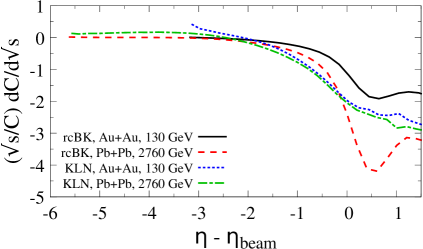
To quantify this effect within the saturation scenario, we have plotted this variable for the rcBK model developed in andre2 , where the non-linear gluon evolution is solved numerically, as well as the KLN model kln which paramterizes the qualitative features of this evolution extrapolating from mid-rapidity. The normalization was performed with the data of the centrality dependence of charged particle multiplicity at mid-rapidity at 2.76 TeV alice276 . The result is plotted in Fig. 10. As can be seen, the dynamics is qualitatively similar to scenario (b) of Fig 1, with the normalized rapidity density smoothly reaching the universal limit. In rcBK this limit is reached slightly sooner than in KLN, although the scaling is not perfect in either. This confirms earlier results published on this topic jamal ; stasto , as well as predictions in jeon (Fig. 8).

However, one should keep in mind that the reason is that the rcBK results reach to the $\eta_{beam}$ region is conditional on the numerical limitation in the rcBK case, since the gluon distribution function has to be extrapolated for $x>0.01$, which is exactly the kinematical regime where one of the hadrons is probed in the fragmentation region, where a significant quark admixture is present. It is reasonable to believe, however, that an additional admixture of sources not present at mid-rapidity would weaken the scaling. In addition, of course, the $k_{T}$ factorization scenario of Eq. 23 and saturation in general are, by an order of magnitude estimate, likely to break down at lower RHIC energies, where experimentally limiting fragmentation works quite well (as Fig. 8 and the accompanying discussion showed), and, for that matter, the calculation of Fig. 10, if taken “literally”, seems to reproduce this fact.

In this spirit, the rcBK calculation done here should be considered as an “lower limit” to limiting fragmentation violation within the CGC scenario, in the sense that this calculation is likely to be rather inaccurate at many energies and rapidities, but deviations from it are likely to break limiting fragmentation. And, comparing different system sizes LHC and bottom RHIC energies of Fig. 10, even in the ideal scenario the breaking of limiting fragmentation would be substantial.

Figure 10: (color online) $dN/d\eta$ and $N_{part}^{-1}d^{2}N/d\eta^{2}$ calculated in KLN (panel (a),(c)) and rcBK (panel (b),(d)) scenarios. The normalization was adjusted to reproduce the data in alice276 using the usual parton-hadron duality parameters

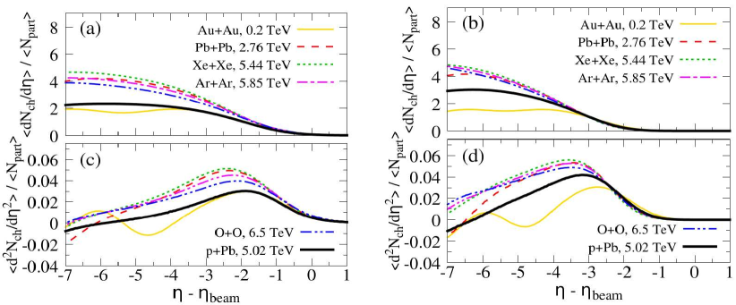
Putting the results of Fig. 10 into the form of Fig. 7 and 8 is shown in Fig. 11. We confirm that the deviation from limiting fragmentation in these models is higher than the data, and surprisingly also of the Glauber model when normalized.

Figure 11: (color online) Violation of limiting fragmentation quantified in the way of Fig 7 and 8 in the KLN and rcBK models

So, what conclusions would we draw if it is found to hold, quantitatively, for pA, dA and AA collisions up to LHC energies? Given the success of the wounded quark model, we could combine it with partonic limiting fragmentation insights to calculate rapidity-dependent “wounded partons”, the number of partons that experienced at least one collision. Without resort to non-perturbative physics, it is difficult to justify this model, since particle production is thought to be perturbative in the regime where partons are good degrees of freedom, and perturbative dynamics does not scale with participants. That said, since wide rapidity intervals correspond to wide spacetime rapidity intervals the idea that confinement effects seep into the longitudinal evolution of partons, and hence “wounded partons” become relevant, is not so unreasonable. Since, phenomenologically, a wounded quark model appears to work woundq1 ; woundq2 ; woundq3 ; woundq4 well enough that fusing this with the geometrical deep inelastic scattering warrants a try.

Using the usual formula for the number of wounded nucleons adapted to the wounded parton picture, with the Fourier transform of the transverse participant density of nucleus $A$

$$\ \tilde{N}_{part}^{qA}(x_{A},k_{A},A,B)\simeq A(x_{A})\tilde{T}_{A}(k_{A},x_{A})\int d^{2}k_{B}dx_{B}\times$$

$$\times\left(1-\left(1-\frac{\tilde{T}_{B}\left(k_{A}-k_{B},x_{B}\right)}{\left(k_{A}-k_{B}\right)^{2}}\right)^{B(x_{B})}\right)$$ (25)

If one introduces the emission function woundq5 for a wounded parton characterized by $x_{A},k_{A}$ to emit a particle of $p_{T},y$ as $F(p_{T},y,k_{A},x_{A})$ one can get the multiplicity in terms of the wounded partons.

For each nucleon collision we will have

$$\frac{dN}{dy}=\int p_{T}dp_{T}dkdxF(p_{T},y,k,x)\times$$ (26)

$$\ \times\left(\tilde{N}_{part}^{qA}(x,k,A,B)+\tilde{N}_{part}^{qB}(x,k,B,A)\right)$$

Expanding to first order in $\tilde{T}_{B}(k)/k^{2}$ it is possible to reduce this expression into a sum of terms of the form

$$\ \frac{dN}{dy}\sim\int p_{T}dp_{T}\int dx_{A}k_{A}dk_{A}A(x_{A})\tilde{T}(k_{A},x_{A})\times$$

$$\times F(p_{T},y,k_{A},x_{A})\int dx_{B}k_{B}dk_{B}\frac{B(x_{B})\tilde{T}_{B}(k_{A}-k_{B},x_{B})}{\left(k_{A}-k_{B}\right)^{2}}$$

assumption (b), together with the reasonable requirement that $B(x\rightarrow 0)$ does not diverge will remove the second integral to an approximate constant value for each nucleon. Assumption (c) ensures $F(p_{T},y,k,x)\simeq F(p_{T},y,k,e^{y})$ and also that $k_{A}-k_{B}\simeq k_{A}$. Additionally assuming the equivalent of (b) and (c) for $F(...)$, i.e. that it is only a narrowly peaked and normalized function of $y$ differences, will ensure the resulting function will only depend on $e^{-y}$ analogously with Eq. 23. Hence, limiting fragmentation is recovered.

Unlike the Color Glass, however, one can straight-forwardly extend limiting fragmentation to $AA$. What prevented limiting fragmentation in the wounded nucleon model was the fact that $f=1$ in Eq. 5 is incompatible with any choice of $\alpha$ in equation 6 that fits multiplicity at mid-rapidity. Physically wounded partons, by allowing participants to be spread across $x$ and nuclear size to vary across $x$, make it possible to combine a purely participant $f=1$ scaling (which does not depend on $\sqrt{s}$) with strongly non-logarithmic dependence of multiplicity per participant, obtained through variation with $x$ of $A(x)$ and $\tilde{T}(x)$. The difference with the Color Glass is that $\tilde{T}(x)$ would still be individual nuclear collisions, albeit with a size that effectively depends in Bjorken $x$. Thus, one expects $Q_{s}(x)$ (“s” is size and not saturation here!) to be independent of the number of participants, leading to a universal $N_{part}^{-1}d^{2}N/d\eta^{2}$.

Previous literature on wounded quarks woundq1 ; woundq2 ; woundq3 ; woundq4 ; woundq5 considers nucleon transverse substructure but does not separate it into $x-$distributions. This allows the authors to fit mid-rapidity data or rapidity data at a given energy. Generalizing these models along the lines presented in this work while maintaining the current phenomenological agreements seems like a straight-forward exercise, albeit one beyond the scope of this paper. Thus, if an eventual confirmation of a $N_{part}^{-1}d^{2}N/d\eta^{2}$ universal across energies and system sizes will indeed be observed, the wounded parton model will be a promising avenue to model this.

IV discussion and summary

In this work, we have examined the behavior of $N_{part}^{-1}d^{2}N/d\eta^{2}$, the multiplicity density per participant, at high rapidity, motivated by the near independence with energy of its first derivative. The universal behavior of $N_{part}^{-1}d^{2}N/d\eta^{2}$ was found to generally break in a Glauber model, particularly in the two-component models usually used to fit data at mid-rapidity. Thus, this is a good observable to constrain such models.

The reason these models fail is physically very simple: Inasmuch as both collisions and participants contribute to multiplicity, the energy dependence of the two factors is non-trivial and generically different from the rapidity dependence. This means that the height of the distribution depends non-trivially on the energy while the width is constrained by kinematics. Absent unnatural cancellations, limiting fragmentation should be broken.

The only way to restore it is to make multiplicity dependence entirely driven by wounded nucleons at all energies. This is however not enough, since the price for this is to make the multiplicity per nucleon in $AA$ collisions rise with energy much faster than logarithmically. This, as well as clashing with experimental data below LHC, will generally break limiting fragmentation as well. A “wounded parton model” might be able to evade such a constraint since there the “size of the wounded degree of freedom”, instead of being encoded in the cross-section, is allowed to vary with longitudinal $x$, which in this case is tightly correlated with momentum rapidity. Energy and rapidity distributions are therefore naturally correlated in this regime. The observation of a universal $N_{part}^{-1}d^{2}N/d\eta^{2}$ could be indicative of “wounded quark” dynamics.

One can ask how universal is the class of models reproducing such universality. Models such as the Color Glass stasto share some similarities with the wounded parton scenario considered in the previous section, but there nuclei lose their individuality and $Q_{s}$ is common to the same area of transverse space (“s” in color glass models is saturation instead of size!). Also, Eq. 23($k_{T}$ factorization) used to connect the gluon density to particle density in this regime leads to a universal slope in the fragmentation region in the same way as Bjorken scaling.

Indeed, as stasto finds approximate limiting fragmentation, explained by the factorization of parton distributions in target and projectile at large rapidities together with the fact that the multiplicity distribution is directly proportional to the parton density in the target and relatively independent of the scales of the process. The wounded parton model conjectured in the previous section shares these characteristics. We note, however, that stasto predicts some violation of limiting fragmentation inasmuch as the assumptions above cease to have validity. Thus, the calculations of stasto point to some violation of $N_{part}^{-1}d^{2}N/d\eta^{2}$, which turns out to be comparable, if not larger, than the Glauber model.

Looking at schee1 ; schee2 ; groz a similar discussion can be made about AdS/CFT initial states, where the breaking of scaling appears even stronger as it is controlled both by a critical transparency and the coupling constant. Thus, some breaking of limiting fragmentation, when all energies and systems sizes are concerned, appears likely in all models claiming connection to field theory (the wounded parton model so far does not).

We continue with experimental considerations. To our knowledge, so far measurements at high enough rapidity to compare to even top RHIC energy were not done, with the closest experimental measurement being alicey ; cmsy ; atlasy . Also, a result, seeming to confirm scenario (b) of Fig. 1, was obtained for $dE_{T}/d\eta$ by the CMS collaboration using the CASTOR detector castor . Since multiplicity and transverse energy have a non-trivial separate dependence which is also sensitive to system size alicept , we hesitate at drawing conclusions there. alicephoton , in contrast to CASTOR, has reported a breaking of limiting fragmentation in inclusive photons. While QED processes are not expected to limiting fragment (there is no hadronization, and $y\sim\ln(1/x)$ is not expected to hold), some 85$\%$ of photons in alicephoton are thought to come from $\pi^{0}$ decays cosentino . Hence, this result makes a breaking of limiting fragmentation at LHC energies likely. In summary, until a direct measurement of both $dN/d\eta$ and $dE_{T}/d\eta$ is performed, relying on these data to make a conclusive statement is difficoult.

Studies comparing the rapidity dependence of p-Pb and Pb-Pb are totally lacking. Comparing with smaller asymmetric systems, such as Pb-Pb and p-Pb collisions, where a deviation from purely wounded dynamics should be more pronounced the observable can be studied on the “same side”, as discussed in jeon .

The fact that most experiments focus the detector on mid-rapidity of course makes this measurement problematic. We want to point out, however, that this is a bulk observable, not requiring particle identification or momentum measurement, problematic since particles at high rapidity are highly relativistic. The existing small experiments at rapidity comparable to lower RHIC energiestotem ; lhcf as well as LHCb lhcb could take part in this investigation together with the larger collaborations.

Since the calculations here were focused on proof-of-concept estimates testing for violation, we will give a “cartoon” of what we expect in each scenario, with the the alternatives are summarized in Fig. 1. The key is to go to a high enough rapidity as to compare with a lower energy. If limiting fragmentation still holds, $N_{part}^{-1}d^{2}N/d\eta^{2}$ will evolve to smoothly “touch” the corresponding value at mid-rapidity of that energy (scenario (b) of Fig. 1). Otherwise, the slopes will be different.

In this paper, we have limited ourselves to multiplicity, which, given a low-viscosity nearly isentropic fluid evolution, can be considered to be an initial state effect molnar . However, past experimental results also reported to have seen limiting fragmentation for elliptic flow at RHIC energies phobosrev . This is considered to be a final state effect, sensitive primarily to the transport coefficients and freeze-out dynamics of the system weakly . Should limiting fragmentation of flow observables, or even of average transverse momentum, be confirmed at the LHC, especially in events of same eccentricity but different size, one might have to rethink this paradigm and start exploring scenarios where “flow” arises as an initial state effect gambini ; raju ; bierlich in the systems concerned.

In conclusion, we have examined limiting fragmentation in various phenomenological models, namely Glauber, Color Glass, and wounded quarks. Glauber models generally fail to reproduce limiting fragmentation at LHC energy once they were tuned to reproduce LHC data. The same is true for Color Glass models once different system sizes are considered. We have further argued that wounded parton scenarios have the potential to model limiting fragmentation also at LHC energies and for all system sizes. Since such limiting fragmentation has not to date been verified, no such model can be considered to have been ruled out. Rather, this paper motivates an experimental search for this observable, and generally for a comparison between low-energy bulk observables and the high rapidity limit of the same observable at high energy. We eagerly away these experimental results.

Acknowledgements GT acknowledges support from FAPESP proc. 2017/06508-7, partecipation in FAPESP tematico 2017/05685-2 and CNPQ bolsa de produtividade 301996/2014-8. DM was supported by CNPQ graduate fellowship n. 147435/2014-5. This work is a part of the project INCT-FNA Proc. No. 464898/2014-5. We thank Fernando Navarra, Radoslaw Ryblewski, Mauro Rogerio Cosentino and Wit Busza for fruitful discussions and suggestions. A.V.G. acknowledges the Brazilian funding agency FAPESP for financial support through grants 2017/14974-8 and 2018/23677-0.

Appendix A A note on rapidity and pseudorapidity

Figure 12: (color online) Estimated distribution of $(y-\eta)/y$ for protons (panel (a)) and $\pi$ (panel (b)) assuming $\left\langle p_{T}\right\rangle$ does not deviate from its mid-rapidity value.

We note that the experimental observable usually measured here is not rapidity (the $z$ direction, where momentum is $p_{z}$. The total momentum is $p$)

$$y=tanh^{-1}\left(\frac{p_{z}}{\sqrt{p^{2}+m^{2}}}\right)$$ (27)

but the pseudo-rapidity, a function of the angle with the beam axis which does not require particle identification

$$\eta=tanh^{-1}\left(\frac{p_{z}}{p}\right)$$ (28)

The rapidity is the observable with the “nice“ transformation property of being linear under boosts. It is also related to Bjorken $x$ by eq. 3 and equal to the space-time rapidity in the Boost-invariant limit (Eq. 18). However, it is very difficoult to measure for ultra-relativistic particles as it requires particle identification, and/or the simultaneus measurement of the energy and momentum.

The pseudo-rapidity has no “nice“ properties, but it is very easy to measure as it is directly related to the longitudinal angle $\theta$

$$\eta=-\ln\tan\left(\frac{\theta}{2}\right)$$ (29)

At mid-rapidity, binning the distribution in terms of $\eta$ rather than $y$ causes the near-gaussian distribution measured in whitebrahms to aquire a ”plateau” necessitating a double gaussian fit, as was done in ampt .

Away for mid-rapidity , for the great majority of produced particles, the two are interchangeable,

$$\eta-y\sim-\mathcal{O}\left(\frac{m^{6}p_{z}^{3}}{p^{9}}\right)\simeq\frac{\cos\theta}{2}\left(\frac{m}{p_{T}}\right)^{2}$$ (30)

In this work we do not fit the rapidity distribution globally, but rather rather concentrate on observables local in rapidity sensitive to limiting fragmentation: the slope in the fragmentation region

$$\left|y\right|\geq\mathcal{O}\left(\frac{1}{2}-\frac{3}{4}\right)\left|y_{0}\right|$$ (31)

and its derivative w.r.t. $\sqrt{s}$. Hence, we assume differences between $y$ and $\eta$ to be negligible.

To estimate the goodness of this assumption, lacking particle identification and $p_{T}$ measurements away from mid-rapidity, we shall take a limiting fragmentation inspired rapidity distribution jeon

$$\frac{dN}{p_{T}dp_{T}dy}=C\left(\ln\left[\frac{\sqrt{s}}{m_{p}}\right]-y\right)\exp\left[-\frac{p_{T}}{2\left\langle p_{T}\right\rangle}\right]$$ (32)

where

$$\ \left\langle p_{T}\right\rangle=\left\{\begin{array}[]{cc}500\mathrm{MeV}&\pi\\ 1\mathrm{GeV}&p\end{array}\right.\phantom{A},\phantom{A}C\simeq 0.65$$

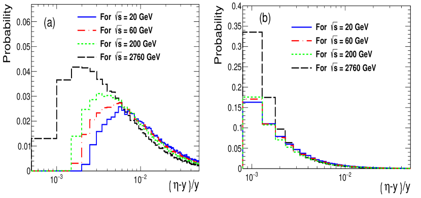
and histogram $(\eta-y)/y$. The results are shown in Fig. 12 for protons and pions, in the region of rapidity considered in the rest of the paper, $y_{0}-y\leq 6$ or so (the figure should be symmetrized if both “target“ and “projectile“ are considered) and assuming a thermal transverse $p_{T}$ distribution with $\left\langle p_{T}\right\rangle$ weakly dependent on rapidity (central values are as in starscan ). As can be seen any reasonable admixture between baryons and mesons will result in a systematic error of order of a percent if $\eta$ and $y$. This error is significantly lower than other experimental errors, and hence is neglected in this work.

To correct this would require a rapidity as well as the energy dependence of the temperature, baryo-chemical potential and $\left\langle p_{T}\right\rangle$, something currently unknown (measured very partially in whitebrahms and starscan ), but, in the spirit of the rest of the paper, any non-trivial variation of this is likely to spoil limiting fragmentation.

The observables treated in this paper, defined around the second derivative of the rapidity distribution away from mid-rapidity, are optimized to minimize the effect of the rapidity-pseudo rapidity interchange. Alternatively, for example, analyzing the width of the rapidity distribution as a whole (as was done, for example, in ampt ) is much more sensitive to this distinction, since the mid-rapidity plateau varies significantly between $\eta$ and $y$, and this influences both the height the width of the distribution in a particle-dependent manner (see becrap for a discussion of this issue at low energies).

References

- (1) J. E. Elias, W. Busza, C. Halliwell, D. Luckey, P. Swartz, L. Votta and C. Young, Phys. Rev. D 22, 13 (1980). doi:10.1103/PhysRevD.22.13
- (2) W. Busza, J. E. Elias, D. F. Jacobs, P. A. Swartz, C. C. Young and M. R. Sogard, Phys. Rev. Lett. 34, 836 (1975). doi:10.1103/PhysRevLett.34.836
- (3) J. Benecke, T. T. Chou, C. N. Yang and E. Yen, Phys. Rev. 188, 2159 (1969). doi:10.1103/PhysRev.188.2159
- (4) F. Halzen and A. D. Martin, New York, USA: Wiley ( 1984) 396p
- (5) B. B. Back et al. [PHOBOS Collaboration], Phys. Rev. C 74, 021901 (2006) doi:10.1103/PhysRevC.74.021901 [nucl-ex/0509034].
- (6) B. B. Back et al., Phys. Rev. Lett. 91, 052303 (2003) doi:10.1103/PhysRevLett.91.052303 [nucl-ex/0210015].
- (7) B. B. Back et al., Nucl. Phys. A 757, 28 (2005) doi:10.1016/j.nuclphysa.2005.03.084 [nucl-ex/0410022].
- (8) I. Arsene et al. [BRAHMS Collaboration], perspective Nucl. Phys. A 757, 1 (2005)
- (9) S. Jeon, V. Topor Pop and M. Bleicher, Phys. Rev. C 69, 044904 (2004) doi:10.1103/PhysRevC.69.044904 [nucl-th/0309077].
- (10) P. Steinberg, Acta Phys. Hung. A 24, 51 (2005) doi:10.1556/APH.24.2005.1-4.8 [nucl-ex/0405022].
- (11) W. Busza, Nucl. Phys. A 854, 57 (2011) doi:10.1016/j.nuclphysa.2010.12.015 [arXiv:1102.3921 [nucl-ex]].
- (12) J. Jalilian-Marian, Phys. Rev. C 70, 027902 (2004) doi:10.1103/PhysRevC.70.027902 [nucl-th/0212018].
- (13) F. Gelis, A. M. Stasto and R. Venugopalan, Eur. Phys. J. C 48, 489 (2006) doi:10.1140/epjc/s10052-006-0020-x [hep-ph/0605087].
- (14) F. O. Duraes, A. V. Giannini, V. P. Goncalves and F. S. Navarra, Phys. Rev. C 89, no. 3, 035205 (2014) doi:10.1103/PhysRevC.89.035205 [arXiv:1401.7888 [hep-ph]].
- (15) A. Dumitru, A. V. Giannini, M. Luzum and Y. Nara, Phys. Lett. B 784, 417 (2018) doi:10.1016/j.physletb.2018.08.028 [arXiv:1805.02702 [hep-ph]].
- (16) Z. W. Lin, C. M. Ko, B. A. Li, B. Zhang and S. Pal, Phys. Rev. C 72, 064901 (2005) doi:10.1103/PhysRevC.72.064901 [nucl-th/0411110].
- (17) P. Sahoo, P. Pareek, S. K. Tiwari and R. Sahoo, Phys. Rev. C 99, no. 4, 044906 (2019) doi:10.1103/PhysRevC.99.044906 arXiv:1803.05155 [hep-ph].
- (18) A. Capella, U. Sukhatme, C. I. Tan and J. Tran Thanh Van, Phys. Rept. 236, 225 (1994). doi:10.1016/0370-1573(94)90064-7
- (19) P. Brogueira, J. Dias de Deus and C. Pajares, Phys. Rev. C 75, 054908 (2007) doi:10.1103/PhysRevC.75.054908 [hep-ph/0605148].
- (20) I. Bautista, C. Pajares, J. G. Milhano and J. Dias de Deus, Phys. Rev. C 86, 034909 (2012) doi:10.1103/PhysRevC.86.034909 [arXiv:1206.6737 [nucl-th]].
- (21) B. Kellers and G. Wolschin, PTEP 2019, 053 doi:10.1093/ptep/ptz044 [arXiv:1901.06421 [hep-ph]].
- (22) G. Torrieri, Phys. Rev. C 82, 054906 (2010) doi:10.1103/PhysRevC.82.054906 [arXiv:0911.4775 [nucl-th]].
- (23) G. Torrieri, EPJ Web Conf. 13, 04002 (2011) doi:10.1051/epjconf/20111304002 [arXiv:1012.2790 [nucl-th]].
- (24) S. Acharya et al. [ALICE Collaboration], arXiv:1805.04432 [nucl-ex].
- (25) M. L. Miller, K. Reygers, S. J. Sanders and P. Steinberg, Ann. Rev. Nucl. Part. Sci. 57, 205 (2007) doi:10.1146/annurev.nucl.57.090506.123020 [nucl-ex/0701025].
- (26) C. Loizides, J. Nagle and P. Steinberg, SoftwareX 1-2, 13 (2015) doi:10.1016/j.softx.2015.05.001 [arXiv:1408.2549 [nucl-ex]].
- (27) Maestrado thesis, Fernando Sartorelli Borcsik, Unicamp
- (28) K. Werner, Phys. Rev. Lett. 98, 152301 (2007) doi:10.1103/PhysRevLett.98.152301 [arXiv:0704.1270 [nucl-th]].
- (29) J. Adam et al. [ALICE Collaboration], Phys. Lett. B 772, 567 (2017) doi:10.1016/j.physletb.2017.07.017 [arXiv:1612.08966 [nucl-ex]].
- (30) A. M. Sirunyan et al. [CMS Collaboration], arXiv:1902.03603 [hep-ex].
- (31) G. Aad et al. [ATLAS Collaboration], Phys. Lett. B 710, 363 (2012) doi:10.1016/j.physletb.2012.02.045 [arXiv:1108.6027 [hep-ex]].
- (32) J. T. Mitchell, D. V. Perepelitsa, M. J. Tannenbaum and P. W. Stankus, Phys. Rev. C 93, no. 5, 054910 (2016) doi:10.1103/PhysRevC.93.054910 [arXiv:1603.08836 [nucl-ex]].
- (33) A. Adare et al. [PHENIX Collaboration], Phys. Rev. C 93, no. 2, 024901 (2016) doi:10.1103/PhysRevC.93.024901 [arXiv:1509.06727 [nucl-ex]].
- (34) R. Nouicer, Eur. Phys. J. C 49, 281 (2007) doi:10.1140/epjc/s10052-006-0128-z [nucl-th/0608038].
- (35) P. Bożek, W. Broniowski and M. Rybczyński, Phys. Rev. C 94, no. 1, 014902 (2016) doi:10.1103/PhysRevC.94.014902 [arXiv:1604.07697 [nucl-th]].
- (36) M. Barej, A. Bzdak and P. Gutowski, arXiv:1904.01435 [hep-ph].
- (37) R. G. Arnold et al., Phys. Rev. Lett. 52, 727 (1984). doi:10.1103/PhysRevLett.52.727
- (38) M. Aaboud et al. [ATLAS Collaboration], Phys. Rev. Lett. 117, no. 18, 182002 (2016) doi:10.1103/PhysRevLett.117.182002 [arXiv:1606.02625 [hep-ex]].
- (39) P. Romatschke and U. Romatschke, Phys. Rev. Lett. 99, 172301 (2007) doi:10.1103/PhysRevLett.99.172301 [arXiv:0706.1522 [nucl-th]].
- (40) S. J. Brodsky, J. F. Gunion and J. H. Kuhn, Phys. Rev. Lett. 39, 1120 (1977). doi:10.1103/PhysRevLett.39.1120
- (41) Y. V. Kovchegov and K. Tuchin, Phys. Rev. D 65, 074026 (2002) doi:10.1103/PhysRevD.65.074026 [hep-ph/0111362].
- (42) D. Kharzeev, E. Levin and M. Nardi, Nucl. Phys. A 747, 609 (2005) doi:10.1016/j.nuclphysa.2004.10.018 [hep-ph/0408050].
- (43) K. Aamodt et al. [ALICE Collaboration], Phys. Rev. Lett. 105, 252301 (2010) doi:10.1103/PhysRevLett.105.252301 [arXiv:1011.3916 [nucl-ex]].
- (44) J. Casalderrey-Solana, M. P. Heller, D. Mateos and W. van der Schee, Phys. Rev. Lett. 111, 181601 (2013) doi:10.1103/PhysRevLett.111.181601 [arXiv:1305.4919 [hep-th]].
- (45) J. Casalderrey-Solana, M. P. Heller, D. Mateos and W. van der Schee, Phys. Rev. Lett. 112, no. 22, 221602 (2014) doi:10.1103/PhysRevLett.112.221602 [arXiv:1312.2956 [hep-th]].
- (46) S. Grozdanov and W. van der Schee, Phys. Rev. Lett. 119, no. 1, 011601 (2017) doi:10.1103/PhysRevLett.119.011601 [arXiv:1610.08976 [hep-th]].
- (47) A. M. Sirunyan et al. [CMS Collaboration], [arXiv:1812.04095 [hep-ex]].
- (48) B. B. Abelev et al. [ALICE Collaboration], Phys. Lett. B 727, 371 (2013) doi:10.1016/j.physletb.2013.10.054 [arXiv:1307.1094 [nucl-ex]].
- (49) B. B. Abelev et al. [ALICE Collaboration], Eur. Phys. J. C 75, no. 4, 146 (2015) doi:10.1140/epjc/s10052-015-3356-2 [arXiv:1411.4981 [nucl-ex]].
- (50) We thank Mauro Cosentino for pointing this out
- (51) T. Csörgő [TOTEM Collaboration], EPJ Web Conf. 206, 06004 (2019) doi:10.1051/epjconf/201920606004 arXiv:1903.06992 [hep-ex].
- (52) O. Adriani et al. [LHCf Collaboration], JHEP 1811, 073 (2018) doi:10.1007/JHEP11(2018)073 [arXiv:1808.09877 [hep-ex]].
- (53) Y. Zhang [LHCb Collaboration], arXiv:1605.07509 [hep-ex].
- (54) A. Dumitru, E. Molnar and Y. Nara, Phys. Rev. C 76, 024910 (2007) doi:10.1103/PhysRevC.76.024910 [arXiv:0706.2203 [nucl-th]].
- (55) C. Aidala et al. [PHENIX Collaboration], Nature Phys. 15, no. 3, 214 (2019) doi:10.1038/s41567-018-0360-0
- (56) G. Gambini and G. Torrieri, Eur. Phys. J. A 53, no. 1, 17 (2017) doi:10.1140/epja/i2017-12205-x [arXiv:1606.07865 [nucl-th]].
- (57) C. Bierlich, Nucl. Phys. A 982, 499 (2019) doi:10.1016/j.nuclphysa.2018.07.015 [arXiv:1807.05271 [nucl-th]].
- (58) K. Dusling, M. Mace and R. Venugopalan, Phys. Rev. Lett. 120, no. 4, 042002 (2018) doi:10.1103/PhysRevLett.120.042002 [arXiv:1705.00745 [hep-ph]].
- (59) L. Adamczyk et al. [STAR Collaboration], Phys. Rev. C 96, no. 4, 044904 (2017) doi:10.1103/PhysRevC.96.044904 [arXiv:1701.07065 [nucl-ex]].
- (60) F. Becattini, J. Cleymans, A. Keranen, E. Suhonen and K. Redlich, Phys. Rev. C 64, 024901 (2001) doi:10.1103/PhysRevC.64.024901 [hep-ph/0002267].