\newsiamremark

remarkRemark \newsiamremarkhypothesisHypothesis \newsiamthmclaimClaim \headersAposteriori Error Estimates for CutFEM with Boundary Correction

A Posteriori Error Estimates with Boundary Correction for a Cut Finite Element Method

Erik Burman Department of Mathematics, University College London, Gower Street, London, UK–WC1E 6BT, United Kingdom () e.burman@ucl.ac.uk    Cuiyu He Department of Mathematics, University College London, Gower Street, London, UK–WC1E 6BT, United Kingdom () c.he@ucl.ac.uk    Mats G. Larson Department of Mathematics and Mathematical Statistics, Umeå University, SE-90187 Umeå, Sweden () mats.larson@umu.se
Abstract

In this work we study a residual based a posteriori error estimation for the CutFEM method applied to an elliptic model problem. We consider the problem with non-polygonal boundary and the analysis takes into account the geometry and data approximation on the boundary. The reliability and efficiency are theoretically proved. Moreover, constants are robust with respect to how the domain boundary cuts the mesh.

keywords:
CutFEM, A Posteriori Error Estimation, AMR
{AMS}

68Q25, 68R10, 68U05

1 Introduction

Meshing and re-meshing procedures remain an important challenge in computational methods, since they can be very computationally expensive for the finite element methods, particularly for problems with complex geometries and interfaces that move during the computational process. Several methods have been invented to alleviating the meshing procedure of the exact domain. Fictitious domain methods were introduced in the finite element context in the papers by Glowinski et al. Glowinski & Pan, (1992) and unfitted finite element methods in the works by Barrett and Elliott Barrett & Elliott, (1984).

Since these seminal works many approaches have been suggested on how to integrate the geometry data in finite element computations in a way that reduces the meshing effort. For instance the fat boundary method by Bertoluzza et al. Bertoluzza et al. , (2005), the fictitious domain methods using Lagrange multipliers inspired by extended finite element methods, pioneered by Haslinger and Renard Haslinger & Renard, (2009), Burman & Hansbo, (2010), or the cut finite element method using Nitsche’s method, introduced by Hansbo and Hansbo and further developed in the fictitious domain framework by various authors Hansbo & Hansbo, (2002), Burman, (2010), Embar et al. , (2010), Becker et al. , (2011), Burman & Hansbo, (2012).

Cut finite element methods have been extensively studied in the recent years, both in the context of interface problems and for fictitious domain methods Burman et al. , (2015b). We restrict the discussion herein to the fictitious domain case. The methodology alleviates the meshing process by employing a background mesh that can be highly structured and letting the domain boundary cut through the elements of the mesh. In cells cut by the boundary the equations are integrated only on the intersection of the element with the physical domain. The boundary conditions are then imposed either using Lagrange multipliers or Nitsche’s method and stability with respect to the cut may be ensured using a ghost penalty stabilization Burman, (2010). The method was originally designed for continuous approximation spaces, but has been adapted for various other methods, e.g, Discontinuous Galerkin method Johansson & Larson, (2013), Gürkan & Massing, (2019), Hybrid High order Methods Burman & Ern, (2019) or Isogeometric analysis Elfverson et al. , (2018). It has been applied to a number of different partial differential equations, e.g, incompressible elasticity/Stokes’ equations Burman & Hansbo, (2014), Massing et al. , (2014b), Burman et al. , (2015a), Guzmán & Olshanskii, (2018), linear elasticity Hansbo et al. , (2017), Helmholtz equations Swift, (2018), time dependent parabolic problems on moving domains Hansbo et al. , (2015), Oseen’s problem Massing et al. , (2018), Winter et al. , (2018) and other fluid models Schott & Wall, (2014), Schott et al. , (2016). It has also been applied successfully to shape optimization problems Burman et al. , (2017, 2018b), Bernland et al. , (2018) and other advanced engineering applications Bui et al. , (2019).

Typically, in cut finite element methods, a domain with curved boundary is approximated using a piecewise affine boundary approximation. This gives a sufficiently good geometry approximation for piecewise affine elements, but if higher order elements are used the geometry approximation must be improved. To alleviate the integration problem resulting from the elements cut by curved boundaries, isoparametric techniques Lehrenfeld, (2017) and so called boundary value correction techniques have been proposed Burman et al. , (2018a), Boiveau et al. , (2018). For both these cases optimal order a priori error estimates for arbitrary order of the polynomial approximation have been derived. For an analysis of the fitted finite element method on domains with curved boundaries we refer to Bramble & King, (1994).

The purpose of this paper is to design an a posteriori error estimation for the cut finite element method for problems with non-polygonal boundary. We will base our discussion on the cut finite element methods for the Poisson problem introduced by Burman and Hansbo Burman & Hansbo, (2012). This method uses Nitsche’s method Nitsche, (1971) to impose Dirichlet boundary conditions and a ghost penalty term Burman, (2010) to enhance stability in the boundary zone. We restrict the discussion to the fictitious domain problem and piecewise affine approximation. The main motivation for studying the a posteriori error estimation is for the application of adaptive mesh refinement (AMR) procedure. It is well known that AMR is extremely useful for problems with singularities, discontinuities, sharp derivatives, etc. and it has been extensively studied in the last two decades, Verfürth, (1994), Ainsworth & Oden, (2011). However, there is very limited work in the literature that takes the geometry approximation into account. In Dörfler & Rumpf, (1998) the a posteriori error estimation is studied for the conforming finite element method on curved boundary where the boundary vertices of the approximated mesh must be located on the true boundary and it is assumed that data can be requested at any point on the boundary and inside the domain, i.e., there is only approximation of the geometry. In Ainsworth & Rankin, (2017) a fully computable error bound is provided for the conforming linear elements with pure Neumann data. To the author’s knowledge there is no existing work on the a posteriori error estimation for cut finite element methods on problems with curved boundary, to allow for. Another approach for the handling of geometric singularities in the cutFEM framework was recently proposed in Jonsson et al. , (2019).

In our error analysis we do not assume that the vertices of the approximation boundary are located on the boundary of the continuous problem, while we do require that the discrete boundary is a sufficiently good approximation of the boundary of the continuous problem. We do not require that data inside the domain can be everywhere requested but only those originally provided in the continuous setting. For the formulation it is necessary to extend the source term data from the domain of the continuous problem to the computational domain, the extension must satisfy certain stability properties. The error estimator comprises two parts. One part is due to the numerical approximation; and the other part is exclusively due to the boundary approximation. We refer to this latter contribution as the boundary correction error. This part must be computed using a locally improved boundary approximation in the boundary zone. The computation of this correction is discussed in the numerical section.

Unlike the methods whose mesh is an exact partition of the computational domain, one major challenge for cut finite element is that the approximated domain cuts the background mesh in an arbitrary way. Because of this the classical efficiency analysis, i.e., by applying the local elementary bubble functions, is not robust. Therefore we divide the efficiency part of the estimates in two parts. The residuals in the bulk, away from the boundary, are estimated in the ordinary fashion. For the residuals in the cut elements and the nonconforming ghost penalty operator, we instead prove a global lower bound of best approximation type, showing that the boundary residuals are bounded by the best approximation of u𝑢u in the physical domain and oscillations.

This paper is organized as follows. In Section 2 the model problem and the cut finite element method is introduced. The error estimator is introduced in Section 3 and as well its global reliability. The local efficiency is proved in Section 4. Finally, we show the results of several numerical experiment in Section 5.

2 Model Problem and the Cut Finite Element Method

2.1 The Continuous Problem

Let ΩΩ\Omega be a domain in dsuperscript𝑑\mathbb{R}^{d} with Lipschitz continuous, piecewise smooth boundary ΩΩ\partial\Omega and exterior unit normal 𝒏𝒏\boldsymbol{n}.

We consider the problem: find u:Ω:𝑢Ωu:\Omega\rightarrow\mathbb{R} such that

(2.1) ΔuΔ𝑢\displaystyle-\Delta u =fabsent𝑓\displaystyle=f\qquad in ΩΩ\Omega
(2.2) u𝑢\displaystyle u =gabsent𝑔\displaystyle=g\qquad on ΩΩ\partial\Omega

where fL2(Ω)𝑓superscript𝐿2Ωf\in L^{2}(\Omega) and gH1/2(Ω)𝑔superscript𝐻12Ωg\in H^{1/2}(\partial\Omega) are given data. It follows from the Lax-Milgram lemma that there exists a unique solution uH1(Ω)𝑢superscript𝐻1Ωu\in H^{1}(\Omega) to this problem. We also have the following elliptic regularity estimate

(2.3) uHs+2(Ω)fHs(Ω),1ss0formulae-sequenceless-than-or-similar-tosubscriptnorm𝑢superscript𝐻𝑠2Ωsubscriptnorm𝑓superscript𝐻𝑠Ω1𝑠subscript𝑠0\|u\|_{H^{s+2}(\Omega)}\lesssim\|f\|_{H^{s}(\Omega)},\qquad-1\leq s\leq s_{0}

for some s01/2subscript𝑠012s_{0}\geq 1/2 depending on the domain. Here and below we use the notation less-than-or-similar-to\lesssim to denote less or equal up to a generic constant that is independent of the mesh-geometry configuration.

2.2 The Mesh, Discrete Domains, and Finite Element Spaces

Assume that ΩΩ\partial\Omega is composed of a finite number of smooth surfaces ΓisubscriptΓ𝑖\Gamma_{i}, such that Ω=iΓ¯iΩsubscript𝑖subscript¯Γ𝑖\partial\Omega=\cup_{i}\bar{\Gamma}_{i}. We let ρ𝜌\rho be the signed distance function, negative on the inside and positive on the outside, to ΩΩ\partial\Omega and we let Uδ(Ω)subscript𝑈𝛿ΩU_{\delta}(\partial\Omega), for δ>0𝛿0\delta>0, be the tubular neighborhood {𝒙d:|ρ(𝒙)|<δ}conditional-set𝒙superscript𝑑𝜌𝒙𝛿\{\boldsymbol{x}\in\mathbb{R}^{d}:|\rho(\boldsymbol{x})|<\delta\} of ΩΩ\partial\Omega. Let Ω0dsubscriptΩ0superscript𝑑\Omega_{0}\subset\mathbb{R}^{d} be a polygonal domain such that Uδ0(Ω)Ω0subscript𝑈subscript𝛿0ΩsubscriptΩ0U_{\delta_{0}}(\Omega)\subset\Omega_{0} where δ0subscript𝛿0\delta_{0} is chosen such that ρ𝜌\rho is well defined in Uδ0(Ω)subscript𝑈subscript𝛿0ΩU_{\delta_{0}}(\Omega). Let 𝒯0,hsubscript𝒯0{\mathcal{T}}_{0,h} be a partition of Ω0subscriptΩ0\Omega_{0} into shape regular triangles or tetrahedra. Note that this setting allows meshes with locally dense refinement.

Given a subset ω𝜔\omega of Ω0subscriptΩ0\Omega_{0}, let 𝒯h(ω)subscript𝒯𝜔{\mathcal{T}}_{h}(\omega) be the submesh defined by

(2.4) 𝒯h(ω)={K𝒯0,h:K¯ω¯}subscript𝒯𝜔conditional-set𝐾subscript𝒯0¯𝐾¯𝜔{\mathcal{T}}_{h}(\omega)=\{K\in{\mathcal{T}}_{0,h}:\overline{K}\cap\overline{\omega}\neq\emptyset\}

i.e., the submesh consisting of elements that intersect ω¯¯𝜔\overline{\omega}, and let

(2.5) h(ω)=K𝒯h(ω)Ksubscript𝜔subscript𝐾subscript𝒯𝜔𝐾\triangle_{h}(\omega)=\bigcup\limits_{K\in{\mathcal{T}}_{h}(\omega)}K

be the union of all elements in 𝒯h(ω)subscript𝒯𝜔{\mathcal{T}}_{h}(\omega).

For each 𝒯0,hsubscript𝒯0{\mathcal{T}}_{0,h} let ΩhsubscriptΩ\Omega_{h} be a polygonal domain approximating ΩΩ\Omega and we assume that ΩhUδ0(Ω)subscriptΩsubscript𝑈subscript𝛿0Ω\partial\Omega_{h}\subset U_{\delta_{0}}(\partial\Omega) which implies that ΩhsubscriptΩ\partial\Omega_{h} is within the distance of δ0subscript𝛿0\delta_{0} to ΩΩ\partial\Omega. We assume neither ΩhΩsubscriptΩΩ\Omega_{h}\subset\Omega nor ΩΩhΩsubscriptΩ\Omega\subset\Omega_{h}, instead the maximum distance between the two domains has to be small enough.

Let the active mesh be defined by

(2.6) 𝒯h:=𝒯h(ΩΩh)assignsubscript𝒯subscript𝒯ΩsubscriptΩ{\mathcal{T}}_{h}:={\mathcal{T}}_{h}({\Omega}\cup\Omega_{h})

i.e., the submesh consisting of elements that intersect ΩhΩsubscriptΩΩ\Omega_{h}\cup\Omega, and let

(2.7) h:=h(ΩΩh)assignsubscriptsubscriptΩsubscriptΩ\triangle_{h}:=\triangle_{h}(\Omega\cup\Omega_{h})

be the union of all elements in 𝒯hsubscript𝒯{\mathcal{T}}_{h}. Since ΩhsubscriptΩ\partial{\Omega}_{h} does not necessarily fit the mesh we denote by 𝒯hbsuperscriptsubscript𝒯𝑏{\mathcal{T}}_{h}^{b} the set of elements that are “cut” by ΩhsubscriptΩ\partial{\Omega}_{h},

𝒯hb={K𝒯0,h:KΩh}𝒯h.superscriptsubscript𝒯𝑏conditional-set𝐾subscript𝒯0𝐾subscriptΩsubscript𝒯{\mathcal{T}}_{h}^{b}=\{K\in{\mathcal{T}}_{0,h}:K\cap\partial{\Omega}_{h}\neq\emptyset\}\subset{\mathcal{T}}_{h}.

We assume that ΩhsubscriptΩ\Omega_{h} is constructed in such a way that for each K𝒯hb𝐾superscriptsubscript𝒯𝑏K\in{\mathcal{T}}_{h}^{b}, the intersection KΩh𝐾subscriptΩK\cap\partial\Omega_{h} is a subset of a d1𝑑1d-1 dimensional hyperplane, i.e., a line segment in two dimensions and a subset of a plane in three dimensions. Under the smallness assumption of hh, for any element K𝒯hb𝐾superscriptsubscript𝒯𝑏K\in{\mathcal{T}}_{h}^{b} there exists an element K𝒯h(Ωh)𝒯hbsuperscript𝐾subscript𝒯subscriptΩsuperscriptsubscript𝒯𝑏K^{\prime}\in{\mathcal{T}}_{h}(\Omega_{h})\setminus{\mathcal{T}}_{h}^{b} such that dist(K,K)=O(h)dist𝐾superscript𝐾𝑂\mbox{dist}(K,K^{\prime})=O(h) where O()𝑂O(\cdot) denotes the big ordo. This is always possible for small enough hh since ΩΩ\Omega is Lipschitz.

Also we denote by {\mathcal{E}} the set of all facets on 𝒯hsubscript𝒯{\mathcal{T}}_{h} and by Isubscript𝐼{\mathcal{E}}_{I}\subset{\mathcal{E}} the set of all interior facets with respect to 𝒯hsubscript𝒯{\mathcal{T}}_{h}. For each F𝐹F\in{\mathcal{E}} denote by 𝒏Fsubscript𝒏𝐹\boldsymbol{n}_{F} an unit vector normal to F𝐹F and by hFsubscript𝐹h_{F} the diameter of F𝐹F. For each K𝒯h𝐾subscript𝒯K\in{\mathcal{T}}_{h} denote by hKsubscript𝐾h_{K} the diameter of K𝐾K and by Ksubscript𝐾{\mathcal{E}}_{K} the set of all facets of K𝐾K.

On the boundary ΩhsubscriptΩ\partial{\Omega}_{h} let 𝒏hsubscript𝒏\boldsymbol{n}_{h} be the outer normal to ΩhsubscriptΩ\partial{\Omega}_{h}. For each ΩhsubscriptΩ\Omega_{h} we assume that, for δ0subscript𝛿0\delta_{0} small enough, there exist functions 𝝂h:Ωhd:subscript𝝂subscriptΩsuperscript𝑑\boldsymbol{\nu}_{h}:\partial\Omega_{h}\rightarrow\mathbb{R}^{d}, |𝝂h|=1subscript𝝂1|\boldsymbol{\nu}_{h}|=1, and ϱh:Ωh:subscriptitalic-ϱsubscriptΩ\varrho_{h}:\partial\Omega_{h}\rightarrow\mathbb{R}, on Uδ0(Ω)subscript𝑈subscript𝛿0ΩU_{\delta_{0}}(\partial\Omega), such that the function 𝒑h(𝒙,ς):=𝒙+ς𝝂h(𝒙)assignsubscript𝒑𝒙𝜍𝒙𝜍subscript𝝂𝒙\boldsymbol{p}_{h}(\boldsymbol{x},\varsigma):=\boldsymbol{x}+\varsigma\boldsymbol{\nu}_{h}(\boldsymbol{x}), is well defined and satisfies 𝒑h(𝒙,ϱh(𝒙))Ωsubscript𝒑𝒙subscriptitalic-ϱ𝒙Ω\boldsymbol{p}_{h}(\boldsymbol{x},\varrho_{h}(\boldsymbol{x}))\in\partial\Omega for all 𝒙Ωh𝒙subscriptΩ\boldsymbol{x}\in\partial\Omega_{h}. The existence of the vector-valued function 𝝂hsubscript𝝂\boldsymbol{\nu}_{h} is known to hold on Lipschitz domains, see Grisvard Grisvard, (2011).

We further assume that 𝒑h(𝒙,ς)Uδ0(Ω)subscript𝒑𝒙𝜍subscript𝑈subscript𝛿0Ω\boldsymbol{p}_{h}(\boldsymbol{x},\varsigma)\in U_{\delta_{0}}(\Omega) for all 𝒙Ωh𝒙subscriptΩ\boldsymbol{x}\in\partial\Omega_{h} and all ς𝜍\varsigma between 00 and ϱh(𝒙)subscriptitalic-ϱ𝒙\varrho_{h}(\boldsymbol{x}). For conciseness we will drop the second argument, ς𝜍\varsigma, of 𝒑hsubscript𝒑\boldsymbol{p}_{h} below whenever it takes the value ϱh(𝒙)subscriptitalic-ϱ𝒙\varrho_{h}(\boldsymbol{x}) and let 𝒑hsubscript𝒑\boldsymbol{p}_{h} denotes the map 𝒑h:ΩhΩ:subscript𝒑subscriptΩΩ\boldsymbol{p}_{h}:\partial\Omega_{h}\rightarrow\partial\Omega. Moreover, we assume that the following assumption is satisfied

(2.8) ϱhL(ΩhK)O(hK)K𝒯hb.formulae-sequencesubscriptnormsubscriptitalic-ϱsuperscript𝐿subscriptΩ𝐾𝑂subscript𝐾for-all𝐾superscriptsubscript𝒯𝑏\|\varrho_{h}\|_{L^{\infty}(\partial\Omega_{h}\cap K)}\leq O(h_{K})\quad\forall\,K\in{\mathcal{T}}_{h}^{b}.

The above assumption immediately implies that ΩhsubscriptΩ\partial{\Omega}_{h} is within the distance of O(h)𝑂O(h) of ΩΩ\partial{\Omega}. More precisely,

(2.9) ϱL(ΩhK)=O(hK)K𝒯hb.formulae-sequencesubscriptnormitalic-ϱsuperscript𝐿subscriptΩ𝐾𝑂subscript𝐾for-all𝐾superscriptsubscript𝒯𝑏\|\varrho\|_{L^{\infty}(\partial\Omega_{h}\cap K)}=O(h_{K})\quad\forall\,K\in{\mathcal{T}}_{h}^{b}.

This assumption is necessary for the constant in the a posteriori error estimates to be independent of the geometry/mesh configuration. It is however not enough to guarantee optimal a priori error estimates, which requires ϱL(ΩhK)O(hK2)subscriptnormitalic-ϱsuperscript𝐿subscriptΩ𝐾𝑂superscriptsubscript𝐾2\|\varrho\|_{L^{\infty}(\partial\Omega_{h}\cap K)}\leq O(h_{K}^{2}), and 𝒏𝒏hL(ΩhK)O(hK)subscriptnorm𝒏subscript𝒏superscript𝐿subscriptΩ𝐾𝑂subscript𝐾\|\boldsymbol{n}-\boldsymbol{n}_{h}\|_{L^{\infty}(\partial\Omega_{h}\cap K)}\leq O(h_{K}), see Burman et al. , (2018a).

2.3 The Cut Finite Element Method

In this subsection we recall the CutFEM introduced in Burman & Hansbo, (2012). We begin with some necessary notation. Let hsubscript\mathcal{F}_{h} be the set of faces intersecting the approximate boundary ΩhsubscriptΩ{\Omega}_{h}:

h={FI:(KFKF)Ωh}subscriptconditional-set𝐹subscript𝐼subscript𝐾𝐹superscriptsubscript𝐾𝐹subscriptΩ\mathcal{F}_{h}=\{F\in{\mathcal{E}}_{I}\,:\,(K_{F}\cup K_{F}^{\prime})\cap\partial{\Omega}_{h}\neq\emptyset\}

where KFsubscript𝐾𝐹K_{F} and KFsubscriptsuperscript𝐾𝐹K^{\prime}_{F} are those two elements sharing F𝐹F as a common facet, and for any discontinuous function v𝑣v define its jump on the facet F𝐹F by

[[v]]|F:=vF+vFandvF±(x)=lims0+v(𝒙s𝒏F).formulae-sequenceassignevaluated-atdelimited-[]delimited-[]𝑣𝐹subscriptsuperscript𝑣𝐹subscriptsuperscript𝑣𝐹andsuperscriptsubscript𝑣𝐹plus-or-minus𝑥subscript𝑠superscript0𝑣minus-or-plus𝒙𝑠subscript𝒏𝐹[\![v]\!]|_{F}:=v^{+}_{F}-v^{-}_{F}\quad\mbox{and}\quad v_{F}^{\pm}(x)=\lim\limits_{s\rightarrow 0^{+}}v(\boldsymbol{x}\mp s\boldsymbol{n}_{F}).

Next define the finite element space

(2.10) Vh:={vH1(h):v|K1(K)K𝒯h}assignsubscript𝑉conditional-set𝑣superscript𝐻1subscriptformulae-sequenceevaluated-at𝑣𝐾subscript1𝐾for-all𝐾subscript𝒯V_{h}:=\{v\in H^{1}(\triangle_{h}):v|_{K}\in\mathbb{P}_{1}(K)\quad\forall\,K\in{\mathcal{T}}_{h}\}

and the forms

(2.11) a0(v,w):=(v,w)ΩhD𝒏hv,wΩhv,D𝒏hwΩh+K𝒯hbβhKv,wΓK,jh(v,w):=γFhhF[[D𝒏Fv]],[[D𝒏Fw]]F,ah(v,w):=a0(v,w)+jh(v,w),lh(w):=(f,w)Ωhgh,D𝒏hwΩh+K𝒯hbβhKgh,wΓK,formulae-sequenceassignsubscript𝑎0𝑣𝑤subscript𝑣𝑤subscriptΩsubscriptsubscript𝐷subscript𝒏𝑣𝑤subscriptΩsubscript𝑣subscript𝐷subscript𝒏𝑤subscriptΩsubscript𝐾superscriptsubscript𝒯𝑏𝛽subscript𝐾subscript𝑣𝑤subscriptΓ𝐾formulae-sequenceassignsubscript𝑗𝑣𝑤𝛾subscript𝐹subscriptsubscript𝐹subscriptdelimited-[]delimited-[]subscript𝐷subscript𝒏𝐹𝑣delimited-[]delimited-[]subscript𝐷subscript𝒏𝐹𝑤𝐹formulae-sequenceassignsubscript𝑎𝑣𝑤subscript𝑎0𝑣𝑤subscript𝑗𝑣𝑤assignsubscript𝑙𝑤subscript𝑓𝑤subscriptΩsubscriptsubscript𝑔subscript𝐷subscript𝒏𝑤subscriptΩsubscript𝐾superscriptsubscript𝒯𝑏𝛽subscript𝐾subscriptsubscript𝑔𝑤subscriptΓ𝐾\begin{split}a_{0}(v,w)&:=(\nabla v,\nabla w)_{\Omega_{h}}-\left<D_{\boldsymbol{n}_{h}}v,w\right>_{\partial\Omega_{h}}-\left<v,D_{\boldsymbol{n}_{h}}w\right>_{\partial\Omega_{h}}+\sum_{K\in{\mathcal{T}}_{h}^{b}}\dfrac{\beta}{h_{K}}\left<v,w\right>_{\Gamma_{K}},\\ j_{h}(v,w)&:=\gamma\sum_{F\in\mathcal{F}_{h}}h_{F}\left<[\![D_{\boldsymbol{n}_{F}}v]\!],[\![D_{\boldsymbol{n}_{F}}w]\!]\right>_{F},\\ a_{h}(v,w)&:=a_{0}(v,w)+j_{h}(v,w),\\ l_{h}(w)&:=(f,w)_{\Omega_{h}}-\left<g_{h},D_{\boldsymbol{n}_{h}}w\right>_{\partial\Omega_{h}}+\sum_{K\in{\mathcal{T}}_{h}^{b}}\dfrac{\beta}{h_{K}}\left<g_{h},w\right>_{\Gamma_{K}},\end{split}

where D𝒏hv:=𝒏hvassignsubscript𝐷subscript𝒏𝑣subscript𝒏𝑣D_{\boldsymbol{n}_{h}}v:=\boldsymbol{n}_{h}\cdot\nabla v, γ𝛾\gamma and β𝛽\beta are positive constants, ghsubscript𝑔g_{h} is an approximation of g𝑔g defined on ΩhsubscriptΩ\partial\Omega_{h}, typically gh(𝒙)=g𝒑hsubscript𝑔𝒙𝑔subscript𝒑g_{h}(\boldsymbol{x})=g\circ\boldsymbol{p}_{h}, and ΓK=KΩhsubscriptΓ𝐾𝐾subscriptΩ\Gamma_{K}=K\cap\partial{\Omega}_{h} and f|ΩhΩevaluated-at𝑓subscriptΩΩf|_{\Omega_{h}\setminus\Omega} is defined by some suitable extension (in the low order case considered here it can be taken to be zero).

Remark 2.1.

The stabilizing term jh(v,w)subscript𝑗𝑣𝑤j_{h}(v,w), which is the so called ghost penalty term, is introduced to extend the coercivity of ah(,)subscript𝑎a_{h}(\cdot,\cdot) to all of hsubscript\triangle_{h}, see Burman, (2010), Massing et al. , (2014a). Thanks to this property one may prove that the condition number of the linear system is uniformly bounded independent of how ΩhsubscriptΩ\Omega_{h} is oriented compared to the mesh.

Remark 2.2.

In order to guarantee the coercivity of Eq. 2.11 β𝛽\beta has to be chosen large enough.

The finite element method is then to find uhVhsubscript𝑢subscript𝑉u_{h}\in V_{h} such that

(2.12) ah(uh,v)=lh(v)vVhformulae-sequencesubscript𝑎subscript𝑢𝑣subscript𝑙𝑣for-all𝑣subscript𝑉a_{h}(u_{h},v)=l_{h}(v)\quad\forall\,v\in V_{h}

where ahsubscript𝑎a_{h} and lhsubscript𝑙l_{h} are defined in Eq. 2.11.

For vH1(Ω0)𝑣superscript𝐻1subscriptΩ0v\in H^{1}({\Omega}_{0}) define the continuous and discrete energy norm respectively by

(2.13) |v|2superscriptnorm𝑣2\displaystyle|\mspace{-1.0mu}|\mspace{-1.0mu}|v|\mspace{-1.0mu}|\mspace{-1.0mu}|^{2} :=vΩ2+D𝒏vH1/2(Ω)2+h12vΩ2assignabsentsubscriptsuperscriptnorm𝑣2Ωsubscriptsuperscriptnormsubscript𝐷𝒏𝑣2superscript𝐻12Ωsubscriptsuperscriptnormsuperscript12𝑣2Ω\displaystyle:=\|\nabla v\|^{2}_{\Omega}+\|D_{\boldsymbol{n}}v\|^{2}_{H^{-1/2}(\partial\Omega)}+\|h^{-\frac{1}{2}}v\|^{2}_{\partial\Omega}

and

(2.14) |v|h2superscriptsubscriptnorm𝑣2\displaystyle|\mspace{-1.0mu}|\mspace{-1.0mu}|v|\mspace{-1.0mu}|\mspace{-1.0mu}|_{h}^{2} :=vΩh2+K𝒯hbhKD𝒏hvΓK2+K𝒯hbhK1vΓK2.assignabsentsubscriptsuperscriptnorm𝑣2subscriptΩsubscript𝐾superscriptsubscript𝒯𝑏subscript𝐾subscriptsuperscriptnormsubscript𝐷subscript𝒏𝑣2subscriptΓ𝐾subscript𝐾superscriptsubscript𝒯𝑏superscriptsubscript𝐾1subscriptsuperscriptnorm𝑣2subscriptΓ𝐾\displaystyle:=\|\nabla v\|^{2}_{\Omega_{h}}+\sum_{K\in{\mathcal{T}}_{h}^{b}}h_{K}\|D_{\boldsymbol{n}_{h}}v\|^{2}_{\Gamma_{K}}+\sum_{K\in{\mathcal{T}}_{h}^{b}}h_{K}^{-1}\|v\|^{2}_{\Gamma_{K}}.

2.4 Some Important Inequalities

We have the following well known inverse and trace inequalities (Di Pietro & Ern,, 2012, Section 1.4.3),

(2.15) vKC(hK1/2vK+hK1/2vK)vH1(K),formulae-sequencesubscriptnorm𝑣𝐾𝐶superscriptsubscript𝐾12subscriptnorm𝑣𝐾superscriptsubscript𝐾12subscriptnorm𝑣𝐾for-all𝑣superscript𝐻1𝐾\|v\|_{\partial K}\leq C(h_{K}^{-1/2}\|v\|_{K}+h_{K}^{1/2}\|\nabla v\|_{K})\quad\forall\,v\in H^{1}(K),
(2.16) hK12vhK+vhKChK1vhKvh1(K)formulae-sequencesuperscriptsubscript𝐾12subscriptnormsubscript𝑣𝐾subscriptnormsubscript𝑣𝐾𝐶superscriptsubscript𝐾1subscriptnormsubscript𝑣𝐾for-allsubscript𝑣subscript1𝐾h_{K}^{-\frac{1}{2}}\|v_{h}\|_{\partial K}+\|\nabla v_{h}\|_{K}\leq Ch_{K}^{-1}\|v_{h}\|_{K}\quad\forall\,v_{h}\in\mathbb{P}_{1}(K)

and Hansbo & Hansbo, (2002)

(2.17) vhΓKC(hK1/2vhK+hK1/2vhK)vh1(K)formulae-sequencesubscriptnormsubscript𝑣subscriptΓ𝐾𝐶superscriptsubscript𝐾12subscriptnormsubscript𝑣𝐾superscriptsubscript𝐾12subscriptnormsubscript𝑣𝐾for-allsubscript𝑣subscript1𝐾\|v_{h}\|_{\Gamma_{K}}\leq C(h_{K}^{-1/2}\|v_{h}\|_{K}+h_{K}^{1/2}\|\nabla v_{h}\|_{K})\quad\forall\,v_{h}\in\mathbb{P}_{1}(K)

where the constant C𝐶C is independent of the relative location of ΩhsubscriptΩ{\Omega}_{h}.

Lemma 1.

Let vH01(Ω)𝑣superscriptsubscript𝐻01Ωv\in H_{0}^{1}({\Omega}). Then for any K𝐾K such that K𝒯hb𝐾superscriptsubscript𝒯𝑏K\in{\mathcal{T}}_{h}^{b} or K(ΩΩh)𝐾ΩsubscriptΩK\cap({\Omega}\setminus{\Omega}_{h})\neq\emptyset there exists a local convex neighborhood 𝒮Ksubscript𝒮𝐾\mathcal{S}_{K} of K𝐾K such that v𝑣v vanishes on a nonzero subset of SKsubscript𝑆𝐾\partial S_{K} and

(2.18) vKhKv𝒮K,less-than-or-similar-tosubscriptnorm𝑣𝐾subscript𝐾subscriptnorm𝑣subscript𝒮𝐾\|v\|_{K}\lesssim h_{K}\|\nabla v\|_{\mathcal{S}_{K}},

where we defined v𝑣v outside ΩΩ{\Omega} using the trivial extension v|Ωc=0evaluated-at𝑣superscriptΩ𝑐0v|_{{\Omega}^{c}}=0.

Proof 2.3.

If KΩc𝐾superscriptΩ𝑐K\subset{\Omega}^{c}, the estimate Eq. 2.18 is obvious since v𝑣v is taken uniformly zero outside ΩΩ{\Omega}. If KΩ𝐾ΩK\cap\partial{\Omega}\neq\emptyset, then we let xKΩ𝑥𝐾Ωx\in K\cap\partial{\Omega} and let SK=Bδ(x)subscript𝑆𝐾subscript𝐵𝛿𝑥S_{K}=B_{\delta}(x) be the open ball centered at x𝑥x with radius δhsimilar-to𝛿\delta\sim h. The estimate (2.18) is a direct consequence of the Poincaré inequality on SKsubscript𝑆𝐾S_{K}. Otherwise KΩ𝐾ΩK\subset{\Omega}. From Eq. 2.8 it follows that

dist(K,Ω)O(h)dist𝐾Ω𝑂\mbox{dist}(K,\partial{\Omega})\leq O(h)

and thus there is xΩ𝑥Ωx\in\partial\Omega and δhsimilar-to𝛿\delta\sim h such that KBδ(x)𝐾subscript𝐵𝛿𝑥K\subset B_{\delta}(x) and now Eq. 2.18 follows with SK=Bδ(x)subscript𝑆𝐾subscript𝐵𝛿𝑥S_{K}=B_{\delta}(x) from the Poincaré inequality on SKsubscript𝑆𝐾S_{K}. This completes the proof of the lemma.

3 Global Reliability

Let e:=uuhassign𝑒𝑢subscript𝑢e:=u-u_{h} and e~~𝑒\tilde{e} be any function such that

e~H1(Ω)ande~|Ω=(guh)formulae-sequence~𝑒superscript𝐻1Ωandevaluated-at~𝑒Ω𝑔subscript𝑢\tilde{e}\in H^{1}({\Omega})\quad\mbox{and}\quad\tilde{e}|_{\partial{\Omega}}=(g-u_{h})

where uhsubscript𝑢u_{h} is the solution to Eq. 2.12.

For each element K𝒯h𝐾subscript𝒯K\in{\mathcal{T}}_{h}, define the local element error indicator ηKsubscript𝜂𝐾\eta_{K} by

(3.1) ηK2=hK2fKΩh2+FKIhF2[[D𝒏Fuh]]F2+hK1ghuhL2(ΓK)2+e~KΩ2.superscriptsubscript𝜂𝐾2superscriptsubscript𝐾2superscriptsubscriptnorm𝑓𝐾subscriptΩ2subscript𝐹subscript𝐾subscript𝐼subscript𝐹2superscriptsubscriptnormdelimited-[]delimited-[]subscript𝐷subscript𝒏𝐹subscript𝑢𝐹2superscriptsubscript𝐾1superscriptsubscriptnormsubscript𝑔subscript𝑢superscript𝐿2subscriptΓ𝐾2superscriptsubscriptnorm~𝑒𝐾Ω2\eta_{K}^{2}=h_{K}^{2}\|f\|_{K\cap{\Omega}_{h}}^{2}+\sum_{F\in{\mathcal{E}}_{K}\cap{\mathcal{E}}_{I}}\dfrac{h_{F}}{2}\|[\![{D_{{\boldsymbol{n}}_{F}}}u_{h}]\!]\|_{F}^{2}+h_{K}^{-1}\|g_{h}-u_{h}\|_{L^{2}(\Gamma_{K})}^{2}+\|\nabla\tilde{e}\|_{K\cap{\Omega}}^{2}.

and let the global error estimator be defined by

(3.2) η=(K𝒯hηK2)1/2.𝜂superscriptsubscript𝐾subscript𝒯superscriptsubscript𝜂𝐾212\eta=\left(\sum_{K\in{\mathcal{T}}_{h}}\eta_{K}^{2}\right)^{1/2}.
Theorem 1.

Let e~H1(Ω)~𝑒superscript𝐻1Ω\tilde{e}\in H^{1}({\Omega}) such that e~|Ω=(guh)|Ωevaluated-at~𝑒Ωevaluated-at𝑔subscript𝑢Ω\tilde{e}|_{\partial{\Omega}}=(g-u_{h})|_{\partial{\Omega}}. We have the following reliability bound

(3.3) eΩCr(K𝒯hηK2+K𝒯hhK2f(ΩΩh)K2)1/2subscriptnorm𝑒Ωsubscript𝐶𝑟superscriptsubscript𝐾subscript𝒯superscriptsubscript𝜂𝐾2subscript𝐾subscript𝒯superscriptsubscript𝐾2superscriptsubscriptnorm𝑓ΩsubscriptΩ𝐾212\|\nabla e\|_{{\Omega}}\leq C_{r}\left(\sum_{K\in{\mathcal{T}}_{h}}\eta_{K}^{2}+\sum_{K\in{\mathcal{T}}_{h}}h_{K}^{2}\|f\|_{({\Omega}\setminus{\Omega}_{h})\cap K}^{2}\right)^{1/2}

where the constant Crsubscript𝐶𝑟C_{r} does not depend on the location of domain-mesh intersection nor the mesh size.

Proof 3.1.

Note that ee~H01(Ω)𝑒~𝑒superscriptsubscript𝐻01Ωe-\tilde{e}\in H_{0}^{1}({\Omega}). By the triangle inequality we have that

(3.4) eΩ(ee~)Ω+e~Ω=supvH01(Ω)((ee~),v)ΩvΩ+e~ΩsupvH01(Ω)(e,v)ΩvΩ+2e~Ω.subscriptdelimited-∥∥𝑒Ωsubscriptdelimited-∥∥𝑒~𝑒Ωsubscriptdelimited-∥∥~𝑒Ωsubscriptsupremum𝑣superscriptsubscript𝐻01Ωsubscript𝑒~𝑒𝑣Ωsubscriptnorm𝑣Ωsubscriptdelimited-∥∥~𝑒Ωsubscriptsupremum𝑣superscriptsubscript𝐻01Ωsubscript𝑒𝑣Ωsubscriptnorm𝑣Ω2subscriptdelimited-∥∥~𝑒Ω\begin{split}\|\nabla e\|_{{\Omega}}&\leq\|\nabla(e-\tilde{e})\|_{{\Omega}}+\|\nabla\tilde{e}\|_{{\Omega}}\\ &=\sup_{v\in H_{0}^{1}({\Omega})}\dfrac{(\nabla(e-\tilde{e}),\nabla v)_{{\Omega}}}{\|\nabla v\|_{{\Omega}}}+\|\nabla\tilde{e}\|_{{\Omega}}\\[5.69054pt] &\leq\sup_{v\in H_{0}^{1}({\Omega})}\dfrac{(\nabla e,\nabla v)_{{\Omega}}}{\|\nabla v\|_{{\Omega}}}+2\|\nabla\tilde{e}\|_{{\Omega}}.\end{split}

It then suffices to show that

supvH01(Ω)(e,v)ΩvΩ(K𝒯hηK2+K𝒯hhK2f(ΩΩh)K2)1/2,less-than-or-similar-tosubscriptsupremum𝑣superscriptsubscript𝐻01Ωsubscript𝑒𝑣Ωsubscriptnorm𝑣Ωsuperscriptsubscript𝐾subscript𝒯superscriptsubscript𝜂𝐾2subscript𝐾subscript𝒯superscriptsubscript𝐾2superscriptsubscriptnorm𝑓ΩsubscriptΩ𝐾212\sup_{v\in H_{0}^{1}({\Omega})}\dfrac{(\nabla e,\nabla v)_{{\Omega}}}{\|\nabla v\|_{{\Omega}}}\lesssim\left(\sum_{K\in{\mathcal{T}}_{h}}\eta_{K}^{2}+\sum_{K\in{\mathcal{T}}_{h}}h_{K}^{2}\|f\|_{({\Omega}\setminus{\Omega}_{h})\cap K}^{2}\right)^{1/2},

which is a direct result from LABEL:{lem:error-rep} and 4 below. This completes the proof of the theorem.

Remark 2.

We omit the second term in Eq. 3.3 in the algorithm computation in order to avoid integration on the curved domain. What’s more, one can easily make it a higher order term by satisfying

ϱL(ΓK)o(hK)K𝒯hb.formulae-sequencesubscriptnormitalic-ϱsuperscript𝐿subscriptΓ𝐾𝑜subscript𝐾for-all𝐾superscriptsubscript𝒯𝑏\|\varrho\|_{L^{\infty}(\Gamma_{K})}\leq o(h_{K})\quad\forall\,K\in{\mathcal{T}}_{h}^{b}.

Lemma 3.

For any vH01(Ω)𝑣superscriptsubscript𝐻01Ωv\in H_{0}^{1}({\Omega}) and vhVhsubscript𝑣subscript𝑉v_{h}\in V_{h} the following equality holds:

(3.5) (e,v)Ω=𝒜1+𝒜2subscript𝑒𝑣Ωsubscript𝒜1subscript𝒜2(\nabla e,\nabla v)_{\Omega}=\mathcal{A}_{1}+\mathcal{A}_{2}

where

(3.6) 𝒜1=(f,vvh)Ωh+(f,v)ΩΩhsubscript𝒜1subscript𝑓𝑣subscript𝑣subscriptΩsubscript𝑓𝑣ΩsubscriptΩ\mathcal{A}_{1}=(f,v-v_{h})_{{\Omega}_{h}}+(f,v)_{{\Omega}\setminus{\Omega}_{h}}

and

(3.7) 𝒜2subscript𝒜2\displaystyle\mathcal{A}_{2} =12K𝒯hFKFΩh[[D𝒏Fuh]](vvh)𝑑s+ghuh,D𝒏hvhΩhabsent12subscript𝐾subscript𝒯subscript𝐹subscript𝐾subscript𝐹subscriptΩdelimited-[]delimited-[]subscript𝐷subscript𝒏𝐹subscript𝑢𝑣subscript𝑣differential-d𝑠subscriptsubscript𝑔subscript𝑢subscript𝐷subscript𝒏subscript𝑣subscriptΩ\displaystyle=-\dfrac{1}{2}\sum_{K\in{\mathcal{T}}_{h}}\sum_{F\in{\mathcal{E}}_{K}}\int_{F\cap{{\Omega}_{h}}}[\![{D_{{\boldsymbol{n}}_{F}}}u_{h}]\!](v-v_{h})\,ds+\left<g_{h}-u_{h},D_{\boldsymbol{n}_{h}}v_{h}\right>_{\partial\Omega_{h}}
12K𝒯hFKF(ΩΩh)[[D𝒏Fuh]]v𝑑s12subscript𝐾subscript𝒯subscript𝐹subscript𝐾subscript𝐹ΩsubscriptΩdelimited-[]delimited-[]subscript𝐷subscript𝒏𝐹subscript𝑢𝑣differential-d𝑠\displaystyle\qquad-\dfrac{1}{2}\sum_{K\in{\mathcal{T}}_{h}}\sum_{F\in{\mathcal{E}}_{K}}\int_{F\cap{({\Omega}\setminus{\Omega}_{h})}}[\![{D_{{\boldsymbol{n}}_{F}}}u_{h}]\!]v\,ds
K𝒯hbβhKghuh,vhΓK+jh(uh,vh).subscript𝐾superscriptsubscript𝒯𝑏𝛽subscript𝐾subscriptsubscript𝑔subscript𝑢subscript𝑣subscriptΓ𝐾subscript𝑗subscript𝑢subscript𝑣\displaystyle\qquad-\sum_{K\in{\mathcal{T}}_{h}^{b}}\dfrac{\beta}{h_{K}}\left<g_{h}-u_{h},v_{h}\right>_{\Gamma_{K}}+j_{h}(u_{h},v_{h}).

Proof 3.2.

Extending vH01(Ω)𝑣subscriptsuperscript𝐻10Ωv\in H^{1}_{0}(\Omega) to dsuperscript𝑑\mathbb{R}^{d} by setting v=0𝑣0v=0 outside of ΩΩ\Omega and using integration by parts gives

(3.8) (e,v)Ω=(f,v)Ω(uh,v)Ωh(uh,v)ΩΩh=(f,v)Ω(uh,vh)Ωh(uh,(vvh))Ωh(uh,v)ΩΩh.subscript𝑒𝑣Ωsubscript𝑓𝑣Ωsubscriptsubscript𝑢𝑣subscriptΩsubscriptsubscript𝑢𝑣ΩsubscriptΩsubscript𝑓𝑣Ωsubscriptsubscript𝑢subscript𝑣subscriptΩsubscriptsubscript𝑢𝑣subscript𝑣subscriptΩsubscriptsubscript𝑢𝑣ΩsubscriptΩ\begin{split}(\nabla e,\nabla v)_{{\Omega}}&=(f,v)_{{\Omega}}-(\nabla u_{h},\nabla v)_{{\Omega}_{h}}-(\nabla u_{h},\nabla v)_{{\Omega}\setminus{\Omega}_{h}}\\[5.69054pt] &=(f,v)_{\Omega}-(\nabla u_{h},\nabla v_{h})_{{\Omega}_{h}}-(\nabla u_{h},\nabla(v-v_{h}))_{{\Omega}_{h}}-(\nabla u_{h},\nabla v)_{{\Omega}\setminus{\Omega}_{h}}.\end{split}

For the second term in Eq. 3.8, by Eq. 2.12 we have

(3.9) (uh,vh)Ωh=D𝒏huh,vhΩh+jh(uh,vh)(f,vh)Ωh+ghuh,D𝒏hvhΩhK𝒯hbβhKghuh,vhΓK.subscriptsubscript𝑢subscript𝑣subscriptΩsubscriptsubscript𝐷subscript𝒏subscript𝑢subscript𝑣subscriptΩsubscript𝑗subscript𝑢subscript𝑣subscript𝑓subscript𝑣subscriptΩsubscriptsubscript𝑔subscript𝑢subscript𝐷subscript𝒏subscript𝑣subscriptΩsubscript𝐾superscriptsubscript𝒯𝑏𝛽subscript𝐾subscriptsubscript𝑔subscript𝑢subscript𝑣subscriptΓ𝐾\begin{split}-(\nabla u_{h},\nabla v_{h})_{{\Omega}_{h}}&=-\left<D_{\boldsymbol{n}_{h}}u_{h},v_{h}\right>_{\partial\Omega_{h}}+j_{h}(u_{h},v_{h})-(f,v_{h})_{\Omega_{h}}\\ &\qquad+\left<g_{h}-u_{h},D_{\boldsymbol{n}_{h}}v_{h}\right>_{\partial\Omega_{h}}-\sum_{K\in{\mathcal{T}}_{h}^{b}}\dfrac{\beta}{h_{K}}\left<g_{h}-u_{h},v_{h}\right>_{\Gamma_{K}}.\end{split}

For the last two terms in (3.8) applying the integration by parts gives

(3.10) (uh,(vvh))Ωh(uh,v)ΩΩh=K𝒯h(KΩh)(D𝒏uh)(vvh)𝑑sK𝒯h(K(ΩΩh))(D𝒏uh)v𝑑s=12K𝒯hFKFΩh[[D𝒏Fuh]](vvh)𝑑s12K𝒯hFKF(ΩΩh)[[D𝒏Fuh]]v𝑑s+D𝒏huh,vhΩh.formulae-sequencesubscriptsubscript𝑢𝑣subscript𝑣subscriptΩsubscriptsubscript𝑢𝑣ΩsubscriptΩsubscript𝐾subscript𝒯subscript𝐾subscriptΩsubscript𝐷𝒏subscript𝑢𝑣subscript𝑣differential-d𝑠subscript𝐾subscript𝒯subscript𝐾ΩsubscriptΩsubscript𝐷𝒏subscript𝑢𝑣differential-d𝑠12subscript𝐾subscript𝒯subscript𝐹subscript𝐾subscript𝐹subscriptΩdelimited-[]delimited-[]subscript𝐷subscript𝒏𝐹subscript𝑢𝑣subscript𝑣differential-d𝑠12subscript𝐾subscript𝒯subscript𝐹subscript𝐾subscript𝐹ΩsubscriptΩdelimited-[]delimited-[]subscript𝐷subscript𝒏𝐹subscript𝑢𝑣differential-d𝑠subscriptsubscript𝐷subscript𝒏subscript𝑢subscript𝑣subscriptΩ\begin{split}&-(\nabla u_{h},\nabla(v-v_{h}))_{{\Omega}_{h}}-(\nabla u_{h},\nabla v)_{{\Omega}\setminus{\Omega}_{h}}\\ &\qquad=-\sum_{K\in{\mathcal{T}}_{h}}\int_{\partial(K\cap{\Omega}_{h})}(D_{\boldsymbol{n}}u_{h})(v-v_{h})\,ds-\sum_{K\in{\mathcal{T}}_{h}}\int_{\partial(K\cap({\Omega}\setminus{\Omega}_{h}))}(D_{\boldsymbol{n}}u_{h})v\,ds\\ &\qquad=-\dfrac{1}{2}\sum_{K\in{\mathcal{T}}_{h}}\sum_{F\in{\mathcal{E}}_{K}}\int_{F\cap{{\Omega}_{h}}}[\![{D_{{\boldsymbol{n}}_{F}}}u_{h}]\!](v-v_{h})\,ds\\ &\qquad\qquad-\dfrac{1}{2}\sum_{K\in{\mathcal{T}}_{h}}\sum_{F\in{\mathcal{E}}_{K}}\int_{F\cap{({\Omega}\setminus{\Omega}_{h})}}[\![{D_{{\boldsymbol{n}}_{F}}}u_{h}]\!]v\,ds+\left<D_{\boldsymbol{n}_{h}}u_{h},v_{h}\right>_{\partial{\Omega}_{h}}.\end{split}

In the last equality we used the following identity

Ωhuh𝒏vds(ΩΩh)uh𝒏vds=0subscriptsubscriptΩsubscript𝑢𝒏𝑣𝑑𝑠subscriptΩsubscriptΩsubscript𝑢𝒏𝑣𝑑𝑠0-\int_{\partial{\Omega}_{h}}\nabla u_{h}\cdot\boldsymbol{n}v\,ds-\int_{\partial({\Omega}\setminus{\Omega}_{h})}\nabla u_{h}\cdot\boldsymbol{n}v\,ds=0

thanks to the fact that v=0𝑣0v=0 on ΩΩ\partial{\Omega} and in ΩhΩsubscriptΩΩ{\Omega}_{h}\setminus{\Omega}, where 𝐧𝐧\boldsymbol{n} without subscript denotes the outer normal to the boundary of domain being integrated. The desired identity Eq. 3.5 is then a direct consequence of Eq. 3.8Eq. 3.10. This completes the proof of the lemma.

Remark 3.3.

Note that 𝒜1subscript𝒜1\mathcal{A}_{1} and 𝒜2subscript𝒜2\mathcal{A}_{2} in 3 does not contain the inconsistency error caused by the boundary approximation. In other words, the boundary correction error has been independently isolated by the term e~norm~𝑒\|\nabla\tilde{e}\|. Since any e~~𝑒\tilde{e} satisfying the boundary condition will yield an upper bound for the error, an inappropriate construction of e~~𝑒\tilde{e} will potentially over estimate the error.

Lemma 4.

Let 𝒜1subscript𝒜1\mathcal{A}_{1} and 𝒜2subscript𝒜2\mathcal{A}_{2} be given in 3. Then we have the following estimates:

(3.11) 𝒜1(K𝒯h(hK2fKΩh2+hK2fK(ΩΩh)2))1/2vΩ,less-than-or-similar-tosubscript𝒜1superscriptsubscript𝐾subscript𝒯superscriptsubscript𝐾2superscriptsubscriptnorm𝑓𝐾subscriptΩ2superscriptsubscript𝐾2superscriptsubscriptnorm𝑓𝐾ΩsubscriptΩ212subscriptnorm𝑣Ω\mathcal{A}_{1}\lesssim\left(\sum_{K\in{\mathcal{T}}_{h}}\left(h_{K}^{2}\|f\|_{K\cap{\Omega}_{h}}^{2}+h_{K}^{2}\|f\|_{K\cap({\Omega}\setminus{\Omega}_{h})}^{2}\right)\right)^{1/2}\|\nabla v\|_{{\Omega}},

and

(3.12) 𝒜2(K𝒯hFKIhF2[[D𝒏Fuh]]F2+K𝒯hbhK1ghuhΓK2)1/2vΩ.less-than-or-similar-tosubscript𝒜2superscriptsubscript𝐾subscript𝒯subscript𝐹subscript𝐾subscript𝐼subscript𝐹2superscriptsubscriptnormdelimited-[]delimited-[]subscript𝐷subscript𝒏𝐹subscript𝑢𝐹2subscript𝐾superscriptsubscript𝒯𝑏superscriptsubscript𝐾1superscriptsubscriptnormsubscript𝑔subscript𝑢subscriptΓ𝐾212subscriptnorm𝑣Ω\mathcal{A}_{2}\lesssim\left(\sum_{K\in{\mathcal{T}}_{h}}\sum_{F\in{\mathcal{E}}_{K}\cap{\mathcal{E}}_{I}}\dfrac{h_{F}}{2}\|[\![{D_{{\boldsymbol{n}}_{F}}}u_{h}]\!]\|_{F}^{2}+\sum_{K\in{\mathcal{T}}_{h}^{b}}h_{K}^{-1}\|g_{h}-u_{h}\|_{\Gamma_{K}}^{2}\right)^{1/2}\|\nabla v\|_{{\Omega}}.

Proof 3.4.

The first term of 𝒜1subscript𝒜1\mathcal{A}_{1} in (3.5) can be bounded directly using the Cauchy-Schwarz inequality and the approximation property of the Scott-Zhang interpolation Scott & Zhang, (1990),

(3.13) (f,vvh)ΩhK𝒯hfKΩhvvhKK𝒯hhKfKΩhvK(K𝒯hhK2fKΩh2)1/2vΩ,subscript𝑓𝑣subscript𝑣subscriptΩsubscript𝐾subscript𝒯subscriptdelimited-∥∥𝑓𝐾subscriptΩsubscriptdelimited-∥∥𝑣subscript𝑣𝐾less-than-or-similar-tosubscript𝐾subscript𝒯subscript𝐾subscriptdelimited-∥∥𝑓𝐾subscriptΩsubscriptdelimited-∥∥𝑣subscript𝐾less-than-or-similar-tosuperscriptsubscript𝐾subscript𝒯superscriptsubscript𝐾2subscriptsuperscriptdelimited-∥∥𝑓2𝐾subscriptΩ12subscriptdelimited-∥∥𝑣Ω\begin{split}(f,v-v_{h})_{{\Omega}_{h}}&\leq\sum_{K\in{\mathcal{T}}_{h}}\|f\|_{K\cap{\Omega}_{h}}\|v-v_{h}\|_{K}\\ &\lesssim\sum_{K\in{\mathcal{T}}_{h}}h_{K}\|f\|_{K\cap{\Omega}_{h}}\|\nabla v\|_{\triangle_{K}}\\ &\lesssim\left(\sum_{K\in{\mathcal{T}}_{h}}h_{K}^{2}\|f\|^{2}_{K\cap{\Omega}_{h}}\right)^{1/2}\|\nabla v\|_{{\Omega}},\end{split}

where Ksubscript𝐾\triangle_{K} is the union of elements in 𝒯hsubscript𝒯{\mathcal{T}}_{h} that shares at least one vertex with K𝐾K.

By Eq. 2.18 the second term of 𝒜1subscript𝒜1\mathcal{A}_{1} can now be bounded as follows:

(3.14) (f,v)ΩΩhK𝒯hfK(ΩΩh)vK(ΩΩh)(K𝒯hhK2fK(ΩΩh)2)1/2vΩ.subscript𝑓𝑣ΩsubscriptΩsubscript𝐾subscript𝒯subscriptdelimited-∥∥𝑓𝐾ΩsubscriptΩsubscriptdelimited-∥∥𝑣𝐾ΩsubscriptΩless-than-or-similar-tosuperscriptsubscript𝐾subscript𝒯superscriptsubscript𝐾2superscriptsubscriptdelimited-∥∥𝑓𝐾ΩsubscriptΩ212subscriptdelimited-∥∥𝑣Ω\begin{split}(f,v)_{{\Omega}\setminus{\Omega}_{h}}&\leq\sum_{K\in{\mathcal{T}}_{h}}\|f\|_{K\cap({\Omega}\setminus{\Omega}_{h})}\|v\|_{K\cap({\Omega}\setminus{\Omega}_{h})}\\ &\lesssim\left(\sum_{K\in{\mathcal{T}}_{h}}h_{K}^{2}\|f\|_{K\cap({\Omega}\setminus{\Omega}_{h})}^{2}\right)^{1/2}\|\nabla v\|_{{\Omega}}.\end{split}

(3.11) is then a direct result of (3.13) and (3.14).

We now proceed to bound terms in 𝒜2subscript𝒜2\mathcal{A}_{2}. The first term of 𝒜2subscript𝒜2\mathcal{A}_{2} can be bounded directly by applying the Cauchy-Schwarz inequality and the approximation property of the Scott-Zhang interpolation,

(3.15) KFKFΩh[[D𝒏Fuh]](vvh)𝑑sKFK[[D𝒏Fuh]]FΩhvvhFKFKhK1/2[[D𝒏Fuh]]FΩhvΔK(KFKhK[[D𝒏Fuh]]FΩh2)1/2vΩ.subscript𝐾subscript𝐹subscript𝐾subscript𝐹subscriptΩdelimited-[]delimited-[]subscript𝐷subscript𝒏𝐹subscript𝑢𝑣subscript𝑣differential-d𝑠subscript𝐾subscript𝐹subscript𝐾subscriptdelimited-∥∥delimited-[]delimited-[]subscript𝐷subscript𝒏𝐹subscript𝑢𝐹subscriptΩsubscriptdelimited-∥∥𝑣subscript𝑣𝐹less-than-or-similar-tosubscript𝐾subscript𝐹subscript𝐾superscriptsubscript𝐾12subscriptdelimited-∥∥delimited-[]delimited-[]subscript𝐷subscript𝒏𝐹subscript𝑢𝐹subscriptΩsubscriptdelimited-∥∥𝑣subscriptΔ𝐾less-than-or-similar-tosuperscriptsubscript𝐾subscript𝐹subscript𝐾subscript𝐾superscriptsubscriptdelimited-∥∥delimited-[]delimited-[]subscript𝐷subscript𝒏𝐹subscript𝑢𝐹subscriptΩ212subscriptdelimited-∥∥𝑣Ω\begin{split}&-\sum_{K}\sum_{F\in{\mathcal{E}}_{K}}\int_{F\cap\Omega_{h}}[\![{D_{{\boldsymbol{n}}_{F}}}u_{h}]\!](v-v_{h})\,ds\\ &\qquad\leq\sum_{K}\sum_{F\in{\mathcal{E}}_{K}}\|[\![{D_{{\boldsymbol{n}}_{F}}}u_{h}]\!]\|_{F\cap\Omega_{h}}\|v-v_{h}\|_{F}\\ &\qquad\lesssim\sum_{K}\sum_{F\in{\mathcal{E}}_{K}}h_{K}^{1/2}\|[\![{D_{{\boldsymbol{n}}_{F}}}u_{h}]\!]\|_{F\cap\Omega_{h}}\|\nabla v\|_{\Delta_{K}}\\ &\qquad\lesssim\left(\sum_{K}\sum_{F\in{\mathcal{E}}_{K}}h_{K}\|[\![{D_{{\boldsymbol{n}}_{F}}}u_{h}]\!]\|_{F\cap\Omega_{h}}^{2}\right)^{1/2}\|\nabla v\|_{{\Omega}}.\end{split}

To bound the second term in 𝒜2subscript𝒜2\mathcal{A}_{2} we apply the trace inequality and Eq. 2.18 that

(3.16) K𝒯hFKF(ΩΩh)[[D𝒏Fuh]]v𝑑sK𝒯hFK[[D𝒏Fuh]]F(ΩΩh)vFK𝒯hFK[[D𝒏Fuh]]F(ΩΩh)(hK1/2vK+hK1/2vK)K𝒯hFKhK1/2[[D𝒏Fuh]]F(ΩΩh)v𝒮K(K𝒯hFKhK[[D𝒏Fuh]]F(ΩΩh)2)1/2vΩ.subscript𝐾subscript𝒯subscript𝐹subscript𝐾subscript𝐹ΩsubscriptΩdelimited-[]delimited-[]subscript𝐷subscript𝒏𝐹subscript𝑢𝑣differential-d𝑠subscript𝐾subscript𝒯subscript𝐹subscript𝐾subscriptdelimited-∥∥delimited-[]delimited-[]subscript𝐷subscript𝒏𝐹subscript𝑢𝐹ΩsubscriptΩsubscriptdelimited-∥∥𝑣𝐹less-than-or-similar-tosubscript𝐾subscript𝒯subscript𝐹subscript𝐾subscriptdelimited-∥∥delimited-[]delimited-[]subscript𝐷subscript𝒏𝐹subscript𝑢𝐹ΩsubscriptΩsuperscriptsubscript𝐾12subscriptdelimited-∥∥𝑣𝐾superscriptsubscript𝐾12subscriptdelimited-∥∥𝑣𝐾less-than-or-similar-tosubscript𝐾subscript𝒯subscript𝐹subscript𝐾superscriptsubscript𝐾12subscriptdelimited-∥∥delimited-[]delimited-[]subscript𝐷subscript𝒏𝐹subscript𝑢𝐹ΩsubscriptΩsubscriptdelimited-∥∥𝑣subscript𝒮𝐾less-than-or-similar-tosuperscriptsubscript𝐾subscript𝒯subscript𝐹subscript𝐾subscript𝐾subscriptsuperscriptdelimited-∥∥delimited-[]delimited-[]subscript𝐷subscript𝒏𝐹subscript𝑢2𝐹ΩsubscriptΩ12subscriptdelimited-∥∥𝑣Ω\begin{split}&-\sum_{K\in{\mathcal{T}}_{h}}\sum_{F\in{\mathcal{E}}_{K}}\int_{F\cap{({\Omega}\setminus{\Omega}_{h})}}[\![{D_{{\boldsymbol{n}}_{F}}}u_{h}]\!]v\,ds\\ &\qquad\leq\sum_{K\in{\mathcal{T}}_{h}}\sum_{F\in{\mathcal{E}}_{K}}\|[\![{D_{{\boldsymbol{n}}_{F}}}u_{h}]\!]\|_{F\cap{({\Omega}\setminus{\Omega}_{h})}}\|v\|_{F}\\ &\qquad\lesssim\sum_{K\in{\mathcal{T}}_{h}}\sum_{F\in{\mathcal{E}}_{K}}\|[\![{D_{{\boldsymbol{n}}_{F}}}u_{h}]\!]\|_{F\cap{({\Omega}\setminus{\Omega}_{h})}}\left(h_{K}^{-1/2}\|v\|_{K}+h_{K}^{1/2}\|\nabla v\|_{K}\right)\\ &\qquad\lesssim\sum_{K\in{\mathcal{T}}_{h}}\sum_{F\in{\mathcal{E}}_{K}}h_{K}^{1/2}\|[\![{D_{{\boldsymbol{n}}_{F}}}u_{h}]\!]\|_{F\cap{({\Omega}\setminus{\Omega}_{h})}}\|\nabla v\|_{\mathcal{S}_{K}}\\ &\qquad\lesssim\left(\sum_{K\in{\mathcal{T}}_{h}}\sum_{F\in{\mathcal{E}}_{K}}h_{K}\|[\![{D_{{\boldsymbol{n}}_{F}}}u_{h}]\!]\|^{2}_{F\cap{({\Omega}\setminus{\Omega}_{h})}}\right)^{1/2}\|\nabla v\|_{{\Omega}}.\end{split}

The jump penalty term in 𝒜2subscript𝒜2\mathcal{A}_{2} can be bounded by applying the Cauchy-Schwarz, triangle, trace, and the inverse inequalities and the stability of the interpolator:

(3.17) jh(uh,vh)γFhhF[[D𝒏Fuh]]F[[D𝒏Fvh]]FFhhF1/2[[D𝒏Fuh]]F(K{KF+,KF}hF1/2vh|KF)FhhF1/2[[D𝒏Fuh]]F(K{KF+,KF}vhK)FhhF1/2[[D𝒏Fuh]]FvF(FhhF[[D𝒏Fuh]]F2)1/2vΩ,subscript𝑗subscript𝑢subscript𝑣𝛾subscript𝐹subscriptsubscript𝐹subscriptdelimited-∥∥delimited-[]delimited-[]subscript𝐷subscript𝒏𝐹subscript𝑢𝐹subscriptdelimited-∥∥delimited-[]delimited-[]subscript𝐷subscript𝒏𝐹subscript𝑣𝐹less-than-or-similar-tosubscript𝐹subscriptsuperscriptsubscript𝐹12subscriptdelimited-∥∥delimited-[]delimited-[]subscript𝐷subscript𝒏𝐹subscript𝑢𝐹evaluated-atsubscript𝐾superscriptsubscript𝐾𝐹superscriptsubscript𝐾𝐹superscriptsubscript𝐹12subscriptdelimited-∥|subscript𝑣𝐾𝐹less-than-or-similar-tosubscript𝐹subscriptsuperscriptsubscript𝐹12subscriptdelimited-∥∥delimited-[]delimited-[]subscript𝐷subscript𝒏𝐹subscript𝑢𝐹subscript𝐾superscriptsubscript𝐾𝐹superscriptsubscript𝐾𝐹subscriptdelimited-∥∥subscript𝑣𝐾less-than-or-similar-tosubscript𝐹subscriptsuperscriptsubscript𝐹12subscriptdelimited-∥∥delimited-[]delimited-[]subscript𝐷subscript𝒏𝐹subscript𝑢𝐹subscriptdelimited-∥∥𝑣subscript𝐹less-than-or-similar-tosuperscriptsubscript𝐹subscriptsubscript𝐹superscriptsubscriptdelimited-∥∥delimited-[]delimited-[]subscript𝐷subscript𝒏𝐹subscript𝑢𝐹212subscriptdelimited-∥∥𝑣Ω\begin{split}j_{h}(u_{h},v_{h})&\leq\gamma\sum_{F\in\mathcal{F}_{h}}h_{F}\|[\![{D_{{\boldsymbol{n}}_{F}}}u_{h}]\!]\|_{F}\|[\![{D_{{\boldsymbol{n}}_{F}}}v_{h}]\!]\|_{F}\\ &\lesssim\sum_{F\in\mathcal{F}_{h}}h_{F}^{1/2}\|[\![{D_{{\boldsymbol{n}}_{F}}}u_{h}]\!]\|_{F}\left(\sum_{K\in\{K_{F}^{+},K_{F}^{-}\}}h_{F}^{1/2}\|\nabla v_{h}|_{K}\|_{F}\right)\\ &\lesssim\sum_{F\in\mathcal{F}_{h}}h_{F}^{1/2}\|[\![{D_{{\boldsymbol{n}}_{F}}}u_{h}]\!]\|_{F}\left(\sum_{K\in\{K_{F}^{+},K_{F}^{-}\}}\|\nabla v_{h}\|_{K}\right)\\ &\lesssim\sum_{F\in\mathcal{F}_{h}}h_{F}^{1/2}\|[\![{D_{{\boldsymbol{n}}_{F}}}u_{h}]\!]\|_{F}\|\nabla v\|_{\triangle_{F}}\\ &\lesssim\left(\sum_{F\in\mathcal{F}_{h}}h_{F}\|[\![{D_{{\boldsymbol{n}}_{F}}}u_{h}]\!]\|_{F}^{2}\right)^{1/2}\|\nabla v\|_{{\Omega}},\end{split}

where KF+(KF)superscriptsubscript𝐾𝐹superscriptsubscript𝐾𝐹K_{F}^{+}(K_{F}^{-}) is the element with 𝐧F(𝐧F)subscript𝐧𝐹subscript𝐧𝐹\boldsymbol{n}_{F}(-\boldsymbol{n}_{F}) being its outer unit normal on F𝐹F and F:=KF+KFassignsubscript𝐹subscriptsuperscriptsubscript𝐾𝐹subscriptsuperscriptsubscript𝐾𝐹\triangle_{F}:=\triangle_{K_{F}^{+}}\cup\triangle_{K_{F}^{-}}.

The remaining two terms in 𝒜2subscript𝒜2\mathcal{A}_{2} can be bounded by applying the Cauchy-Schwarz and trace inequalities, Eq. 2.18 and the stability of the interpolator:

(3.18) K𝒯hbβhKghuh,vhΓK+ghuh,D𝒏hvhΩhK𝒯hb(hK1ghuhΓKvhΓK+ghuhΓKD𝒏hvhΓK)K𝒯hbhK1ghuhΓK(hK1/2vhK+hK1/2vhK)K𝒯hbhK1/2ghuhΓKv𝒮KΔK(K𝒯hbhK1ghuhΓK2)1/2vΩ.less-than-or-similar-tosubscript𝐾superscriptsubscript𝒯𝑏𝛽subscript𝐾subscriptsubscript𝑔subscript𝑢subscript𝑣subscriptΓ𝐾subscriptsubscript𝑔subscript𝑢subscript𝐷subscript𝒏subscript𝑣subscriptΩsubscript𝐾superscriptsubscript𝒯𝑏superscriptsubscript𝐾1subscriptdelimited-∥∥subscript𝑔subscript𝑢subscriptΓ𝐾subscriptdelimited-∥∥subscript𝑣subscriptΓ𝐾subscriptdelimited-∥∥subscript𝑔subscript𝑢subscriptΓ𝐾subscriptdelimited-∥∥subscript𝐷subscript𝒏subscript𝑣subscriptΓ𝐾less-than-or-similar-tosubscript𝐾superscriptsubscript𝒯𝑏superscriptsubscript𝐾1subscriptdelimited-∥∥subscript𝑔subscript𝑢subscriptΓ𝐾superscriptsubscript𝐾12subscriptdelimited-∥∥subscript𝑣𝐾superscriptsubscript𝐾12subscriptdelimited-∥∥subscript𝑣𝐾less-than-or-similar-tosubscript𝐾superscriptsubscript𝒯𝑏superscriptsubscript𝐾12subscriptdelimited-∥∥subscript𝑔subscript𝑢subscriptΓ𝐾subscriptdelimited-∥∥𝑣subscript𝒮𝐾subscriptΔ𝐾less-than-or-similar-tosuperscriptsubscript𝐾superscriptsubscript𝒯𝑏superscriptsubscript𝐾1subscriptsuperscriptdelimited-∥∥subscript𝑔subscript𝑢2subscriptΓ𝐾12subscriptdelimited-∥∥𝑣Ω\begin{split}&\sum_{K\in{\mathcal{T}}_{h}^{b}}\dfrac{\beta}{h_{K}}\left<g_{h}-u_{h},v_{h}\right>_{\Gamma_{K}}+\left<g_{h}-u_{h},D_{\boldsymbol{n}_{h}}v_{h}\right>_{\partial\Omega_{h}}\\ &\qquad\lesssim\sum_{K\in{\mathcal{T}}_{h}^{b}}\left(h_{K}^{-1}\|g_{h}-u_{h}\|_{\Gamma_{K}}\ \|v_{h}\|_{\Gamma_{K}}+\|g_{h}-u_{h}\|_{\Gamma_{K}}\|D_{\boldsymbol{n}_{h}}v_{h}\|_{\Gamma_{K}}\right)\\ &\qquad\lesssim\sum_{K\in{\mathcal{T}}_{h}^{b}}h_{K}^{-1}\|g_{h}-u_{h}\|_{\Gamma_{K}}\left(h_{K}^{-1/2}\|v_{h}\|_{K}+h_{K}^{1/2}\|\nabla v_{h}\|_{K}\right)\\ &\qquad\lesssim\sum_{K\in{\mathcal{T}}_{h}^{b}}h_{K}^{-1/2}\|g_{h}-u_{h}\|_{\Gamma_{K}}\|\nabla v\|_{\mathcal{S}_{K}\cup\Delta_{K}}\\ &\qquad\lesssim\left(\sum_{K\in{\mathcal{T}}_{h}^{b}}h_{K}^{-1}\|g_{h}-u_{h}\|^{2}_{\Gamma_{K}}\right)^{1/2}\|\nabla v\|_{{\Omega}}.\end{split}

Finally, combining (3.15)-(3.18) and the Young’s inequality yields (3.12). This completes the proof of the lemma.

4 Efficiency

In this section we prove the efficiency of the error indicator introduced in Eq. 3.1. For the classical finite element method the efficiency is usually proved in a local fashion by applying the local facet and element bubble functions. For elements that are not intersected with the boundary and whose facets do not belong to the ghost penalty set we are able to prove the efficiency using the classical bubble technique.

Lemma 1.

Let K𝐾K be a given element in 𝒯hsubscript𝒯{\mathcal{T}}_{h} such that K𝒯hb𝐾superscriptsubscript𝒯𝑏K\not\in{\mathcal{T}}_{h}^{b} and Kh=subscript𝐾subscript{\mathcal{E}}_{K}\cap\mathcal{F}_{h}=\emptyset. Then the following local efficiency result holds:

(4.1) ηKCe(uuh)Δ~K,subscript𝜂𝐾subscript𝐶𝑒subscriptnorm𝑢subscript𝑢subscript~Δ𝐾\eta_{K}\leq C_{e}\|\nabla(u-u_{h})\|_{\tilde{\Delta}_{K}},

where Δ~Ksubscript~Δ𝐾\tilde{\Delta}_{K} is a local neighborhood of K𝐾K and the efficiency constant Cesubscript𝐶𝑒C_{e} does not depend on the mesh size nor the domain-mesh intersection.

Proof 4.1.

The proof is classical and we refer Verfürth, (1994), Cai et al. , (2017).

Remark 4.2.

For the regular elements, we take the boundary correction error e~KΩsubscriptnorm~𝑒𝐾Ω\|\nabla\tilde{e}\|_{K\cap{\Omega}} to be 00 since we can always design e~~𝑒\tilde{e} in such a way that it vanishes inside regular elements in order to avoid over-estimation (see Section 5.1).
Refer to caption
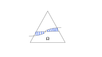
Figure 1: An irregular element K𝐾K and DKsubscript𝐷𝐾D_{K} (the shaded area)

For an element K𝐾K that is irregular, i.e., K𝒯hb𝐾superscriptsubscript𝒯𝑏K\in{\mathcal{T}}_{h}^{b} or Khsubscript𝐾subscript{\mathcal{E}}_{K}\cap\mathcal{F}_{h}\neq\emptyset, applying the same bubble technique for cut elements unfortunately will result in the dependence on the location of domain-mesh intersection. As an alternative we prove the efficiency for the term of ghost penalty as a whole. The efficiency bounds for the element residual on irregular elements can be then also proved with the aid of the efficiency result for the ghost penalty and the numerical scheme.

For each K𝐾K define EK=K((ΩΩh)(ΩΩh))subscript𝐸𝐾𝐾ΩsubscriptΩΩsubscriptΩE_{K}=\partial K\cap((\Omega\cup\Omega_{h})\setminus(\Omega\cap\Omega_{h})) and DK=K((ΩΩh)(ΩΩh))subscript𝐷𝐾𝐾ΩsubscriptΩΩsubscriptΩD_{K}=K\cap((\Omega\cup\Omega_{h})\setminus(\Omega\cap\Omega_{h})), see Fig. 1 for an illustration.

We first prove a discrete Poincare inequality that will be useful in the following efficiency proof.

Lemma 2.

For any vVh𝑣subscript𝑉v\in V_{h} the following estimate is true:

(4.2) K𝒯h(hK2vDK2+hK1vEK2)|v|h2+|vh|jh2,less-than-or-similar-tosubscript𝐾subscript𝒯superscriptsubscript𝐾2superscriptsubscriptnorm𝑣subscript𝐷𝐾2superscriptsubscript𝐾1superscriptsubscriptnorm𝑣subscript𝐸𝐾2subscriptsuperscriptnorm𝑣2subscriptsuperscriptnormsubscript𝑣2subscript𝑗\sum_{K\in{\mathcal{T}}_{h}}(h_{K}^{-2}\|v\|_{D_{K}}^{2}+h_{K}^{-1}\|v\|_{E_{K}}^{2})\lesssim|\mspace{-1.0mu}|\mspace{-1.0mu}|v|\mspace{-1.0mu}|\mspace{-1.0mu}|^{2}_{h}+|\mspace{-1.0mu}|\mspace{-1.0mu}|v_{h}|\mspace{-1.0mu}|\mspace{-1.0mu}|^{2}_{j_{h}},

where |vh|jh2=jh(vh,vh)superscriptsubscriptnormsubscript𝑣subscript𝑗2subscript𝑗subscript𝑣subscript𝑣|\mspace{-1.0mu}|\mspace{-1.0mu}|v_{h}|\mspace{-1.0mu}|\mspace{-1.0mu}|_{j_{h}}^{2}=j_{h}(v_{h},v_{h}).

Proof 4.3.

First, for each K𝐾K such that EK,DKsubscript𝐸𝐾subscript𝐷𝐾E_{K},D_{K}\neq\emptyset, note that using the trace inequality Eq. 2.16 we see that

hK1vEK2hK1vK2hK2vK2.superscriptsubscript𝐾1superscriptsubscriptnorm𝑣subscript𝐸𝐾2superscriptsubscript𝐾1superscriptsubscriptnorm𝑣𝐾2less-than-or-similar-tosuperscriptsubscript𝐾2superscriptsubscriptnorm𝑣𝐾2h_{K}^{-1}\|v\|_{E_{K}}^{2}\leq h_{K}^{-1}\|v\|_{\partial K}^{2}\lesssim h_{K}^{-2}\|v\|_{K}^{2}.

It follows that

hK2vDK2+hK1vEK2hK2vK2.less-than-or-similar-tosuperscriptsubscript𝐾2superscriptsubscriptnorm𝑣subscript𝐷𝐾2superscriptsubscript𝐾1superscriptsubscriptnorm𝑣subscript𝐸𝐾2superscriptsubscript𝐾2superscriptsubscriptnorm𝑣𝐾2h_{K}^{-2}\|v\|_{D_{K}}^{2}+h_{K}^{-1}\|v\|_{E_{K}}^{2}\lesssim h_{K}^{-2}\|v\|_{K}^{2}.

Now observe that there exists a set denoted by SKhsubscript𝑆𝐾subscriptS_{K}\subset\triangle_{h} such that EK,DKSKsubscript𝐸𝐾subscript𝐷𝐾subscript𝑆𝐾E_{K},D_{K}\subset S_{K}, diam(SKΩh)diamsubscript𝑆𝐾subscriptΩ\mbox{diam}(S_{K}\cap{\Omega}_{h}) is of order hKsubscript𝐾h_{K} and for which using Poincaré’s inequality

(4.3) vKhKvSK+KSK0hK1/2vΓK.less-than-or-similar-tosubscriptnorm𝑣𝐾subscript𝐾subscriptnorm𝑣subscript𝑆𝐾subscriptsuperscript𝐾subscript𝑆𝐾0superscriptsubscriptsuperscript𝐾12subscriptnorm𝑣subscriptΓsuperscript𝐾\|v\|_{K}\lesssim h_{K}\|\nabla v\|_{S_{K}}+\sum_{K^{\prime}\cap S_{K}\neq 0}h_{K^{\prime}}^{1/2}\|v\|_{\Gamma_{K^{\prime}}}.

By the equivalence of norms theorem we also have

(4.4) vSKvSKΩh+FIFSKhF1/2[[D𝒏Fv]]F.subscriptnorm𝑣subscript𝑆𝐾subscriptnorm𝑣subscript𝑆𝐾subscriptΩsubscript𝐹subscript𝐼𝐹subscript𝑆𝐾superscriptsubscript𝐹12subscriptnormdelimited-[]delimited-[]subscript𝐷subscript𝒏𝐹𝑣𝐹\|\nabla v\|_{S_{K}}\leq\|\nabla v\|_{S_{K}\cap{\Omega}_{h}}+\sum_{\begin{subarray}{c}F\in{\mathcal{E}}_{I}\\ F\subset S_{K}\end{subarray}}h_{F}^{1/2}\|[\![{D_{{\boldsymbol{n}}_{F}}}v]\!]\|_{F}.

Combining Eq. 4.3 and Eq. 4.4 gives Eq. 4.2. This completes the proof of the lemma.

We assume that for each K𝒯hb𝐾superscriptsubscript𝒯𝑏K\in{\mathcal{T}}_{h}^{b} there exists at least one vertex, say z𝑧z, of K𝐾K such that diam(ωzΩh)=O(hK)diamsubscript𝜔𝑧subscriptΩ𝑂subscript𝐾\mbox{diam}({\omega}_{z}\cap{\Omega}_{h})=O(h_{K}) where ωzsubscript𝜔𝑧{\omega}_{z} is the union of all all elements sharing z𝑧z as a vertex. Define

osc(f)=K(hK2ffzωzΩh2+hK2ffzK(ΩΩh)2)1/2,osc𝑓subscript𝐾superscriptsuperscriptsubscript𝐾2superscriptsubscriptnorm𝑓subscript𝑓𝑧subscript𝜔𝑧subscriptΩ2superscriptsubscript𝐾2superscriptsubscriptnorm𝑓subscript𝑓𝑧𝐾ΩsubscriptΩ212\mbox{osc}(f)=\sum_{K}\left(h_{K}^{2}\|f-f_{z}\|_{{\omega}_{z}\cap{\Omega}_{h}}^{2}+h_{K}^{2}\|f-f_{z}\|_{K\cap({\Omega}\setminus{\Omega}_{h})}^{2}\right)^{1/2},

where fzsubscript𝑓𝑧f_{z} is chosen such that fz=argminchKfcωzΩhsubscript𝑓𝑧subscriptargmin𝑐subscript𝐾subscriptnorm𝑓𝑐subscript𝜔𝑧subscriptΩf_{z}=\mathop{\mathrm{argmin}}_{c\in\mathcal{R}}h_{K}\|f-c\|_{{\omega}_{z}\cap{\Omega}_{h}}. We will now proceed and prove a best approximation result for the element residuals of the cut elements. First we give a Lemma showing that the element residual of a cut element can be bounded by the ghost penalty term, the boundary residual and oscillation in data.

Lemma 4.4.

For each K𝒯hb𝐾superscriptsubscript𝒯𝑏K\in{\mathcal{T}}_{h}^{b} its element residual has the following bound:

(4.5) hKfKΩhFω¯zIhF1/2[[D𝒏Fuh]]FΩh+(KωzhK1uhghΓK2)12+hKffzωzΩh+hKffzK(ΩΩh).less-than-or-similar-tosubscript𝐾subscriptdelimited-∥∥𝑓𝐾subscriptΩsubscript𝐹subscript¯𝜔𝑧subscript𝐼superscriptsubscript𝐹12subscriptdelimited-∥∥delimited-[]delimited-[]subscript𝐷subscript𝒏𝐹subscript𝑢𝐹subscriptΩsuperscriptsubscript𝐾subscript𝜔𝑧superscriptsubscript𝐾1subscriptsuperscriptdelimited-∥∥subscript𝑢subscript𝑔2subscriptΓ𝐾12subscript𝐾subscriptdelimited-∥∥𝑓subscript𝑓𝑧subscript𝜔𝑧subscriptΩsubscript𝐾subscriptdelimited-∥∥𝑓subscript𝑓𝑧𝐾ΩsubscriptΩ\begin{split}h_{K}\|f\|_{K\cap{\Omega}_{h}}\lesssim&\sum_{F\subset\bar{\omega}_{z}\cap{\mathcal{E}}_{I}}h_{F}^{1/2}\|[\![{D_{{\boldsymbol{n}}_{F}}}u_{h}]\!]\|_{F\cap{\Omega}_{h}}+\left(\sum_{K\subset{\omega}_{z}}h_{K}^{-1}\|u_{h}-g_{h}\|^{2}_{\Gamma_{K}}\right)^{\frac{1}{2}}\\ &+h_{K}\|f-f_{z}\|_{{\omega}_{z}\cap{\Omega}_{h}}+h_{K}\|f-f_{z}\|_{K\cap({\Omega}\setminus{\Omega}_{h})}.\end{split}

Proof 4.5.

By the triangle inequality we firstly have

(4.6) hKfKΩhhKffzKΩh+hKfzωzΩh,subscript𝐾subscriptnorm𝑓𝐾subscriptΩsubscript𝐾subscriptnorm𝑓subscript𝑓𝑧𝐾subscriptΩsubscript𝐾subscriptnormsubscript𝑓𝑧subscript𝜔𝑧subscriptΩh_{K}\|f\|_{K\cap{\Omega}_{h}}\leq h_{K}\|f-f_{z}\|_{K\cap{\Omega}_{h}}+h_{K}\|f_{z}\|_{{\omega}_{z}\cap{\Omega}_{h}},

where fzsubscript𝑓𝑧f_{z} at this point can be chosen as any arbitrary constant. Let λzsubscript𝜆𝑧\lambda_{z} be the barycentric hat function associated with z𝑧z then we also have

(4.7) fzωzΩh2fzλz1/2Ωh2=(f,fzλz)Ωh(ffz,fzλz)Ωh.less-than-or-similar-tosubscriptsuperscriptnormsubscript𝑓𝑧2subscript𝜔𝑧subscriptΩsuperscriptsubscriptnormsubscript𝑓𝑧superscriptsubscript𝜆𝑧12subscriptΩ2subscript𝑓subscript𝑓𝑧subscript𝜆𝑧subscriptΩsubscript𝑓subscript𝑓𝑧subscript𝑓𝑧subscript𝜆𝑧subscriptΩ\|f_{z}\|^{2}_{{\omega}_{z}\cap{\Omega}_{h}}\lesssim\|f_{z}\lambda_{z}^{1/2}\|_{{\Omega}_{h}}^{2}=(f,f_{z}\lambda_{z})_{{\Omega}_{h}}-(f-f_{z},f_{z}\lambda_{z})_{{\Omega}_{h}}.

Let wz=fzλzsubscript𝑤𝑧subscript𝑓𝑧subscript𝜆𝑧w_{z}=f_{z}\lambda_{z}. Applying Eq. 2.12 and integration by parts yields

(4.8) (f,fzλz)Ωh=(uh,wz)ΩhD𝒏huh,wzΩhuhgh,D𝒏hwzΩh+K𝒯hbβhKuhgh,wzΓK+γFhhF[[D𝒏Fuh]],[[D𝒏Fwz]]F=Fωz[[D𝒏Fuh]],wzFΩhuhgh,D𝒏hwzΩh+K𝒯hbβhKuhgh,wzΓK+γFhhF[[D𝒏Fuh]],[[D𝒏Fwz]]Fω¯zFωzhF1/2[[D𝒏Fuh]]FΩhfzωzΩh+KωzK𝒯hbhK3/2uhghΓKfzωzΩh+FhFω¯zhF1/2[[D𝒏Fuh]]Fω¯zfzωzΩh.subscript𝑓subscript𝑓𝑧subscript𝜆𝑧subscriptΩsubscriptsubscript𝑢subscript𝑤𝑧subscriptΩsubscriptsubscript𝐷subscript𝒏subscript𝑢subscript𝑤𝑧subscriptΩsubscriptsubscript𝑢subscript𝑔subscript𝐷subscript𝒏subscript𝑤𝑧subscriptΩsubscriptsuperscript𝐾superscriptsubscript𝒯𝑏𝛽subscriptsuperscript𝐾subscriptsubscript𝑢subscript𝑔subscript𝑤𝑧subscriptΓsuperscript𝐾𝛾subscript𝐹subscriptsubscript𝐹subscriptdelimited-[]delimited-[]subscript𝐷subscript𝒏𝐹subscript𝑢delimited-[]delimited-[]subscript𝐷subscript𝒏𝐹subscript𝑤𝑧𝐹subscript𝐹subscript𝜔𝑧subscriptdelimited-[]delimited-[]subscript𝐷subscript𝒏𝐹subscript𝑢subscript𝑤𝑧𝐹subscriptΩsubscriptsubscript𝑢subscript𝑔subscript𝐷subscript𝒏subscript𝑤𝑧subscriptΩsubscriptsuperscript𝐾superscriptsubscript𝒯𝑏𝛽subscriptsuperscript𝐾subscriptsubscript𝑢subscript𝑔subscript𝑤𝑧subscriptΓsuperscript𝐾𝛾subscript𝐹subscriptsubscript𝐹subscriptdelimited-[]delimited-[]subscript𝐷subscript𝒏𝐹subscript𝑢delimited-[]delimited-[]subscript𝐷subscript𝒏𝐹subscript𝑤𝑧𝐹subscript¯𝜔𝑧less-than-or-similar-tosubscript𝐹subscript𝜔𝑧superscriptsubscript𝐹12subscriptdelimited-∥∥delimited-[]delimited-[]subscript𝐷subscript𝒏𝐹subscript𝑢𝐹subscriptΩsubscriptdelimited-∥∥subscript𝑓𝑧subscript𝜔𝑧subscriptΩsubscriptsuperscript𝐾subscript𝜔𝑧superscript𝐾superscriptsubscript𝒯𝑏superscriptsubscriptsuperscript𝐾32subscriptdelimited-∥∥subscript𝑢subscript𝑔subscriptΓsuperscript𝐾subscriptdelimited-∥∥subscript𝑓𝑧subscript𝜔𝑧subscriptΩsubscript𝐹subscript𝐹subscript¯𝜔𝑧superscriptsubscript𝐹12subscriptdelimited-∥∥delimited-[]delimited-[]subscript𝐷subscript𝒏𝐹subscript𝑢𝐹subscript¯𝜔𝑧subscriptdelimited-∥∥subscript𝑓𝑧subscript𝜔𝑧subscriptΩ\begin{split}&(f,f_{z}\lambda_{z})_{{\Omega}_{h}}=(\nabla u_{h},\nabla w_{z})_{\Omega_{h}}-\left<D_{\boldsymbol{n}_{h}}u_{h},w_{z}\right>_{\partial\Omega_{h}}-\left<u_{h}-g_{h},D_{\boldsymbol{n}_{h}}w_{z}\right>_{\partial\Omega_{h}}\\ &+\sum_{K^{\prime}\in{\mathcal{T}}_{h}^{b}}\dfrac{\beta}{h_{K^{\prime}}}\left<u_{h}-g_{h},w_{z}\right>_{\Gamma_{K^{\prime}}}+\gamma\sum_{F\in\mathcal{F}_{h}}h_{F}\left<[\![{D_{{\boldsymbol{n}}_{F}}}u_{h}]\!],[\![{D_{{\boldsymbol{n}}_{F}}}w_{z}]\!]\right>_{F}\\ =&\sum_{F\subset{\omega}_{z}}\left<[\![{D_{{\boldsymbol{n}}_{F}}}u_{h}]\!],w_{z}\right>_{F\cap{\Omega}_{h}}-\left<u_{h}-g_{h},D_{\boldsymbol{n}_{h}}w_{z}\right>_{\partial\Omega_{h}}\\ &+\sum_{K^{\prime}\in{\mathcal{T}}_{h}^{b}}\dfrac{\beta}{h_{K^{\prime}}}\left<u_{h}-g_{h},w_{z}\right>_{\Gamma_{K^{\prime}}}+\gamma\sum_{F\in\mathcal{F}_{h}}h_{F}\left<[\![{D_{{\boldsymbol{n}}_{F}}}u_{h}]\!],[\![{D_{{\boldsymbol{n}}_{F}}}w_{z}]\!]\right>_{F\cap\bar{\omega}_{z}}\\ \lesssim&\sum_{F\subset{\omega}_{z}}h_{F}^{-1/2}\|[\![{D_{{\boldsymbol{n}}_{F}}}u_{h}]\!]\|_{F\cap{\Omega}_{h}}\|f_{z}\|_{{\omega}_{z}\cap{\Omega}_{h}}+\sum_{\begin{subarray}{c}K^{\prime}\subset{\omega}_{z}\\ K^{\prime}\in{\mathcal{T}}_{h}^{b}\end{subarray}}h_{K^{\prime}}^{-3/2}\|u_{h}-g_{h}\|_{\Gamma_{K^{\prime}}}\|f_{z}\|_{{\omega}_{z}\cap{\Omega}_{h}}\\ &+\sum_{\begin{subarray}{c}F\in\mathcal{F}_{h}\\ F\subset\bar{\omega}_{z}\end{subarray}}h_{F}^{-1/2}\|[\![{D_{{\boldsymbol{n}}_{F}}}u_{h}]\!]\|_{F\cap\bar{\omega}_{z}}\|f_{z}\|_{{\omega}_{z}\cap{\Omega}_{h}}.\end{split}

The last inequality utilizes the fact that fzsubscript𝑓𝑧f_{z} is a constant and the trace and inverse inequalities. Combining Eq. 4.7, Eq. 4.8 and the Cauchy Schwarz inequality gives

(4.9) hKfzΩhKFω¯zIhF1/2[[uh𝒏F]]F+(KωzhK1uhghΓK2)12+ffzωzΩh,less-than-or-similar-tosubscript𝐾subscriptdelimited-∥∥subscript𝑓𝑧subscriptΩ𝐾subscript𝐹subscript¯𝜔𝑧subscript𝐼superscriptsubscript𝐹12subscriptdelimited-∥∥delimited-[]delimited-[]subscript𝑢subscript𝒏𝐹𝐹superscriptsubscriptsuperscript𝐾subscript𝜔𝑧superscriptsubscriptsuperscript𝐾1subscriptsuperscriptdelimited-∥∥subscript𝑢subscript𝑔2subscriptΓsuperscript𝐾12subscriptdelimited-∥∥𝑓subscript𝑓𝑧subscript𝜔𝑧subscriptΩ\begin{split}h_{K}\|f_{z}\|_{{\Omega}_{h}\cap K}\lesssim&\sum_{F\subset\bar{\omega}_{z}\cap{\mathcal{E}}_{I}}h_{F}^{1/2}\|[\![\nabla u_{h}\cdot\boldsymbol{n}_{F}]\!]\|_{F}\\ &\qquad+\left(\sum_{K^{\prime}\subset{\omega}_{z}}h_{K^{\prime}}^{-1}\|u_{h}-g_{h}\|^{2}_{\Gamma_{K^{\prime}}}\right)^{\frac{1}{2}}+\|f-f_{z}\|_{{\omega}_{z}\cap{\Omega}_{h}},\end{split}

which, combining with Eq. 4.6, yields Eq. 4.5.

We now prove the main bound for the residuals in the cut elements.

Theorem 3.

Let u𝑢u and uhsubscript𝑢u_{h} be the solution to Eq. 2.1 and Eq. 2.12, respectively. Then the following best approximation result holds:

(4.10) jh(uh,uh)+K𝒯hbhK2fKΩh2CeinfvhVh(|uvh|2+|vh|jh2+K𝒯hbhK1vhghΓK2+osc(f)2).subscript𝑗subscript𝑢subscript𝑢subscript𝐾superscriptsubscript𝒯𝑏superscriptsubscript𝐾2superscriptsubscriptdelimited-∥∥𝑓𝐾subscriptΩ2subscript𝐶𝑒subscriptinfimumsubscript𝑣subscript𝑉superscriptnorm𝑢subscript𝑣2superscriptsubscriptnormsubscript𝑣subscript𝑗2subscript𝐾superscriptsubscript𝒯𝑏superscriptsubscript𝐾1subscriptsuperscriptdelimited-∥∥subscript𝑣subscript𝑔2subscriptΓ𝐾oscsuperscript𝑓2\begin{split}&j_{h}(u_{h},u_{h})+\sum_{K\in{\mathcal{T}}_{h}^{b}}h_{K}^{2}\|f\|_{K\cap{\Omega}_{h}}^{2}\\ \leq&C_{e}\inf_{v_{h}\in V_{h}}\left(|\mspace{-1.0mu}|\mspace{-1.0mu}|u-v_{h}|\mspace{-1.0mu}|\mspace{-1.0mu}|^{2}+|\mspace{-1.0mu}|\mspace{-1.0mu}|v_{h}|\mspace{-1.0mu}|\mspace{-1.0mu}|_{j_{h}}^{2}+\sum_{K\in{\mathcal{T}}_{h}^{b}}h_{K}^{-1}\|v_{h}-g_{h}\|^{2}_{\Gamma_{K}}+\mbox{osc}(f)^{2}\right).\end{split}

where the constant Cesubscript𝐶𝑒C_{e} does not depend on the mesh size nor on the domain-mesh intersection.

Proof 4.6.

By the triangle inequality we have

(4.11) jh(uh,uh)jh(uhvh,uhvh)+jh(vh,vh)less-than-or-similar-tosubscript𝑗subscript𝑢subscript𝑢subscript𝑗subscript𝑢subscript𝑣subscript𝑢subscript𝑣subscript𝑗subscript𝑣subscript𝑣j_{h}(u_{h},u_{h})\lesssim j_{h}(u_{h}-v_{h},u_{h}-v_{h})+j_{h}(v_{h},v_{h})

and

(4.12) K𝒯hbhK1uhghΓK2K𝒯hbhK1uhvhΓK2+K𝒯hbhK1vhghΓKless-than-or-similar-tosubscript𝐾superscriptsubscript𝒯𝑏superscriptsubscript𝐾1superscriptsubscriptnormsubscript𝑢subscript𝑔subscriptΓ𝐾2subscript𝐾superscriptsubscript𝒯𝑏superscriptsubscript𝐾1superscriptsubscriptnormsubscript𝑢subscript𝑣subscriptΓ𝐾2subscript𝐾superscriptsubscript𝒯𝑏superscriptsubscript𝐾1subscriptnormsubscript𝑣subscript𝑔subscriptΓ𝐾\sum_{K\in{\mathcal{T}}_{h}^{b}}h_{K}^{-1}\|u_{h}-g_{h}\|_{\Gamma_{K}}^{2}\lesssim\sum_{K\in{\mathcal{T}}_{h}^{b}}h_{K}^{-1}\|u_{h}-v_{h}\|_{\Gamma_{K}}^{2}+\sum_{K\in{\mathcal{T}}_{h}^{b}}h_{K}^{-1}\|v_{h}-g_{h}\|_{\Gamma_{K}}

Denote by ϕ=uhvhitalic-ϕsubscript𝑢subscript𝑣\phi=u_{h}-v_{h}. Then

jh(uhvh,uhvh)+K𝒯hbhK1uhvhΓK2|ϕ|h2+|ϕ|jh2.subscript𝑗subscript𝑢subscript𝑣subscript𝑢subscript𝑣subscript𝐾superscriptsubscript𝒯𝑏superscriptsubscript𝐾1superscriptsubscriptnormsubscript𝑢subscript𝑣subscriptΓ𝐾2superscriptsubscriptnormitalic-ϕ2superscriptsubscriptnormitalic-ϕsubscript𝑗2j_{h}(u_{h}-v_{h},u_{h}-v_{h})+\sum_{K\in{\mathcal{T}}_{h}^{b}}h_{K}^{-1}\|u_{h}-v_{h}\|_{\Gamma_{K}}^{2}\leq|\mspace{-1.0mu}|\mspace{-1.0mu}|\phi\ |\mspace{-1.0mu}|\mspace{-1.0mu}|_{h}^{2}+|\mspace{-1.0mu}|\mspace{-1.0mu}|\phi|\mspace{-1.0mu}|\mspace{-1.0mu}|_{j_{h}}^{2}.

Applying the coercivity result (see Burman et al. , (2015b)), Eq. 2.11 and Eq. 2.12 gives

(4.13) |ϕ|h2+|ϕ|jh2jh(uhvh,ϕ)+a0(uhvh,ϕ)=lh(ϕ)a0(vh,ϕ)jh(vh,ϕ)=lh(ϕ)(f,ϕ)Ω+(u,ϕ)ΩD𝒏u,ϕΩah(vh,ϕ)jh(vh,ϕ)i=14𝒜i,less-than-or-similar-tosuperscriptsubscriptnormitalic-ϕ2superscriptsubscriptnormitalic-ϕsubscript𝑗2subscript𝑗subscript𝑢subscript𝑣italic-ϕsubscript𝑎0subscript𝑢subscript𝑣italic-ϕsubscript𝑙italic-ϕsubscript𝑎0subscript𝑣italic-ϕsubscript𝑗subscript𝑣italic-ϕsubscript𝑙italic-ϕsubscript𝑓italic-ϕΩsubscript𝑢italic-ϕΩsubscriptsubscript𝐷𝒏𝑢italic-ϕΩsubscript𝑎subscript𝑣italic-ϕsubscript𝑗subscript𝑣italic-ϕsuperscriptsubscript𝑖14subscript𝒜𝑖\begin{split}&|\mspace{-1.0mu}|\mspace{-1.0mu}|\phi|\mspace{-1.0mu}|\mspace{-1.0mu}|_{h}^{2}+|\mspace{-1.0mu}|\mspace{-1.0mu}|\phi|\mspace{-1.0mu}|\mspace{-1.0mu}|_{j_{h}}^{2}\lesssim j_{h}(u_{h}-v_{h},\phi)+a_{0}(u_{h}-v_{h},\phi)\\ &\qquad=l_{h}(\phi)-a_{0}(v_{h},\phi)-j_{h}(v_{h},\phi)\\ &\qquad=l_{h}(\phi)-(f,\phi)_{\Omega}+(\nabla u,\nabla\phi)_{\Omega}-\left<D_{\boldsymbol{n}}u,\phi\right>_{\partial\Omega}-a_{h}(v_{h},\phi)-j_{h}(v_{h},\phi)\\ &\qquad\triangleq\sum_{i=1}^{4}\mathcal{A}_{i},\end{split}

where

𝒜1subscript𝒜1\displaystyle\mathcal{A}_{1} =(f,ϕ)Ωh(f,ϕ)Ω,absentsubscript𝑓italic-ϕsubscriptΩsubscript𝑓italic-ϕΩ\displaystyle=(f,\phi)_{{\Omega}_{h}}-(f,\phi)_{{\Omega}},
𝒜2subscript𝒜2\displaystyle\mathcal{A}_{2} =vhgh,ϕ𝒏ΩhK𝒯hbβhKvhgh,ϕΓK,absentsubscriptsubscript𝑣subscript𝑔italic-ϕ𝒏subscriptΩsubscript𝐾superscriptsubscript𝒯𝑏𝛽subscript𝐾subscriptsubscript𝑣subscript𝑔italic-ϕsubscriptΓ𝐾\displaystyle=\left<v_{h}-g_{h},\nabla\phi\cdot\boldsymbol{n}\right>_{\partial\Omega_{h}}-\sum_{K\in{\mathcal{T}}_{h}^{b}}\dfrac{\beta}{h_{K}}\left<v_{h}-g_{h},\phi\right>_{\Gamma_{K}},
𝒜3subscript𝒜3\displaystyle\mathcal{A}_{3} =(u,ϕ)Ω(vh,ϕ)Ωh+D𝒏hvh,ϕΩhD𝒏u,ϕΩ,absentsubscript𝑢italic-ϕΩsubscriptsubscript𝑣italic-ϕsubscriptΩsubscriptsubscript𝐷subscript𝒏subscript𝑣italic-ϕsubscriptΩsubscriptsubscript𝐷𝒏𝑢italic-ϕΩ\displaystyle=(\nabla u,\nabla\phi)_{\Omega}-(\nabla v_{h},\nabla\phi)_{\Omega_{h}}+\left<D_{\boldsymbol{n}_{h}}v_{h},\phi\right>_{\partial\Omega_{h}}-\left<D_{\boldsymbol{n}}u,\phi\right>_{\partial\Omega},
𝒜4subscript𝒜4\displaystyle\mathcal{A}_{4} =jh(vh,ϕ).absentsubscript𝑗subscript𝑣italic-ϕ\displaystyle=-j_{h}(v_{h},\phi).

To estimate 𝒜1subscript𝒜1\mathcal{A}_{1}, applying the Cauchy-Schwarz inequality and 2 gives

(4.14) 𝒜1(K𝒯hhK2fDK2)1/2(K𝒯hhK2ϕDK2)1/2(K𝒯hhK2fDK2)1/2(|ϕ|h+|ϕ|jh).subscript𝒜1superscriptsubscript𝐾subscript𝒯superscriptsubscript𝐾2superscriptsubscriptdelimited-∥∥𝑓subscript𝐷𝐾212superscriptsubscript𝐾subscript𝒯superscriptsubscript𝐾2superscriptsubscriptdelimited-∥∥italic-ϕsubscript𝐷𝐾212less-than-or-similar-tosuperscriptsubscript𝐾subscript𝒯superscriptsubscript𝐾2superscriptsubscriptdelimited-∥∥𝑓subscript𝐷𝐾212subscriptnormitalic-ϕsubscriptnormitalic-ϕsubscript𝑗\begin{split}\mathcal{A}_{1}&\leq\left(\sum_{K\in{\mathcal{T}}_{h}}h_{K}^{2}\|f\|_{D_{K}}^{2}\right)^{1/2}\left(\sum_{K\in{\mathcal{T}}_{h}}h_{K}^{-2}\|\phi\|_{D_{K}}^{2}\right)^{1/2}\\ &\lesssim\left(\sum_{K\in{\mathcal{T}}_{h}}h_{K}^{2}\|f\|_{D_{K}}^{2}\right)^{1/2}\left(|\mspace{-1.0mu}|\mspace{-1.0mu}|\phi|\mspace{-1.0mu}|\mspace{-1.0mu}|_{h}+|\mspace{-1.0mu}|\mspace{-1.0mu}|\phi|\mspace{-1.0mu}|\mspace{-1.0mu}|_{j_{h}}\right).\end{split}

𝒜2subscript𝒜2\mathcal{A}_{2} can be estimated directly using the Cauchy-Schwarz inequality,

(4.15) 𝒜2(K𝒯hbhK1vhghΓK2)1/2(K𝒯hbhKD𝒏hϕΓK2+K𝒯hbhK1ϕΓK2)1/2(K𝒯hbhK1vhghΓK2)1/2|ϕ|hsubscript𝒜2superscriptsubscript𝐾superscriptsubscript𝒯𝑏superscriptsubscript𝐾1superscriptsubscriptdelimited-∥∥subscript𝑣subscript𝑔subscriptΓ𝐾212superscriptsubscript𝐾superscriptsubscript𝒯𝑏subscript𝐾superscriptsubscriptdelimited-∥∥subscript𝐷subscript𝒏italic-ϕsubscriptΓ𝐾2subscript𝐾superscriptsubscript𝒯𝑏superscriptsubscript𝐾1superscriptsubscriptdelimited-∥∥italic-ϕsubscriptΓ𝐾212less-than-or-similar-tosuperscriptsubscript𝐾superscriptsubscript𝒯𝑏superscriptsubscript𝐾1superscriptsubscriptdelimited-∥∥subscript𝑣subscript𝑔subscriptΓ𝐾212subscriptnormitalic-ϕ\begin{split}\mathcal{A}_{2}&\leq\left(\sum_{K\in{\mathcal{T}}_{h}^{b}}h_{K}^{-1}\|v_{h}-g_{h}\|_{\Gamma_{K}}^{2}\right)^{1/2}\left(\sum_{K\in{\mathcal{T}}_{h}^{b}}h_{K}\|D_{\boldsymbol{n}_{h}}\phi\|_{\Gamma_{K}}^{2}+\sum_{K\in{\mathcal{T}}_{h}^{b}}h_{K}^{-1}\|\phi\|_{\Gamma_{K}}^{2}\right)^{1/2}\\ &\lesssim\left(\sum_{K\in{\mathcal{T}}_{h}^{b}}h_{K}^{-1}\|v_{h}-g_{h}\|_{\Gamma_{K}}^{2}\right)^{1/2}|\mspace{-1.0mu}|\mspace{-1.0mu}|\phi|\mspace{-1.0mu}|\mspace{-1.0mu}|_{h}\end{split}

To estimate 𝒜3subscript𝒜3\mathcal{A}_{3}, add and subtract suitable terms to obtain,

𝒜3=((uvh),ϕ)Ω(uvh)𝒏,ϕΩ+(vh,ϕ)ΩΩh(vh,ϕ)ΩhΩ+vh𝒏,ϕΩhvh𝒏,ϕΩ.subscript𝒜3subscript𝑢subscript𝑣italic-ϕΩsubscript𝑢subscript𝑣𝒏italic-ϕΩsubscriptsubscript𝑣italic-ϕΩsubscriptΩsubscriptsubscript𝑣italic-ϕsubscriptΩΩsubscriptsubscript𝑣𝒏italic-ϕsubscriptΩsubscriptsubscript𝑣𝒏italic-ϕΩ\begin{split}\mathcal{A}_{3}&=(\nabla(u-v_{h}),\nabla\phi)_{\Omega}-\left<\nabla(u-v_{h})\cdot\boldsymbol{n},\phi\right>_{\partial\Omega}\\ &\qquad+(\nabla v_{h},\nabla\phi)_{\Omega\setminus\Omega_{h}}-(\nabla v_{h},\nabla\phi)_{\Omega_{h}\setminus\Omega}+\left<\nabla v_{h}\cdot\boldsymbol{n},\phi\right>_{\partial\Omega_{h}}-\left<\nabla v_{h}\cdot\boldsymbol{n},\phi\right>_{\partial\Omega}.\end{split}

Observe that using integration by parts we have

(vh,ϕ)ΩΩh(vh,ϕ)ΩhΩ+vh𝒏,ϕΩhvh𝒏,ϕΩK𝒯hbEK|[[D𝒏Fvh]]ϕ|𝑑sjh(vh,vh)12(K𝒯hbh12ϕEK2)12jh(vh,vh)12(|ϕ|h+|ϕ|jh)subscriptsubscript𝑣italic-ϕΩsubscriptΩsubscriptsubscript𝑣italic-ϕsubscriptΩΩsubscriptsubscript𝑣𝒏italic-ϕsubscriptΩsubscriptsubscript𝑣𝒏italic-ϕΩsubscript𝐾superscriptsubscript𝒯𝑏subscriptsubscript𝐸𝐾delimited-[]delimited-[]subscript𝐷subscript𝒏𝐹subscript𝑣italic-ϕdifferential-d𝑠subscript𝑗superscriptsubscript𝑣subscript𝑣12superscriptsubscript𝐾superscriptsubscript𝒯𝑏subscriptsuperscriptdelimited-∥∥superscript12italic-ϕ2subscript𝐸𝐾12subscript𝑗superscriptsubscript𝑣subscript𝑣12subscriptnormitalic-ϕsubscriptnormitalic-ϕsubscript𝑗\begin{split}&(\nabla v_{h},\nabla\phi)_{\Omega\setminus\Omega_{h}}-(\nabla v_{h},\nabla\phi)_{\Omega_{h}\setminus\Omega}+\left<\nabla v_{h}\cdot\boldsymbol{n},\phi\right>_{\partial\Omega_{h}}-\left<\nabla v_{h}\cdot\boldsymbol{n},\phi\right>_{\partial\Omega}\\ &\qquad\leq\sum_{K\in\mathcal{T}_{h}^{b}}\int_{E_{K}}|[\![{D_{{\boldsymbol{n}}_{F}}}v_{h}]\!]\phi|\,ds\\ &\qquad\leq j_{h}(v_{h},v_{h})^{\frac{1}{2}}\left(\sum_{K\in\mathcal{T}_{h}^{b}}\|h^{-\frac{1}{2}}\phi\|^{2}_{E_{K}}\right)^{\frac{1}{2}}\\ &\qquad\leq j_{h}(v_{h},v_{h})^{\frac{1}{2}}(|\mspace{-1.0mu}|\mspace{-1.0mu}|\phi|\mspace{-1.0mu}|\mspace{-1.0mu}|_{h}+|\mspace{-1.0mu}|\mspace{-1.0mu}|\phi|\mspace{-1.0mu}|\mspace{-1.0mu}|_{j_{h}})\end{split}

where we used Lemma 2 for the last inequality. Then applying the Cauchy-Schwarz inequality and 2 gives

(4.16) 𝒜3(uvh)ΩϕΩ+D𝒏h(uvh)H1/2(Ω)ϕH1/2(Ω)+jh(vh,vh)12(|ϕ|h+|ϕ|jh)((uvh)Ω+D𝒏h(uvh)H1/2(Ω)+jh(vh,vh)12)(|ϕ|h+|ϕ|jh).subscript𝒜3subscriptdelimited-∥∥𝑢subscript𝑣Ωsubscriptdelimited-∥∥italic-ϕΩsubscriptdelimited-∥∥subscript𝐷subscript𝒏𝑢subscript𝑣superscript𝐻12Ωsubscriptdelimited-∥∥italic-ϕsuperscript𝐻12Ωsubscript𝑗superscriptsubscript𝑣subscript𝑣12subscriptnormitalic-ϕsubscriptnormitalic-ϕsubscript𝑗subscriptdelimited-∥∥𝑢subscript𝑣Ωsubscriptdelimited-∥∥subscript𝐷subscript𝒏𝑢subscript𝑣superscript𝐻12Ωsubscript𝑗superscriptsubscript𝑣subscript𝑣12subscriptnormitalic-ϕsubscriptnormitalic-ϕsubscript𝑗\begin{split}\mathcal{A}_{3}\leq&\|\nabla(u-v_{h})\|_{\Omega}\|\nabla\phi\|_{{\Omega}}+\|D_{\boldsymbol{n}_{h}}(u-v_{h})\|_{H^{-1/2}(\partial\Omega)}\|\phi\|_{H^{1/2}(\partial{\Omega})}\\ &+j_{h}(v_{h},v_{h})^{\frac{1}{2}}(|\mspace{-1.0mu}|\mspace{-1.0mu}|\phi|\mspace{-1.0mu}|\mspace{-1.0mu}|_{h}+|\mspace{-1.0mu}|\mspace{-1.0mu}|\phi|\mspace{-1.0mu}|\mspace{-1.0mu}|_{j_{h}})\\ \leq&(\|\nabla(u-v_{h})\|_{\Omega}+\|D_{\boldsymbol{n}_{h}}(u-v_{h})\|_{H^{-1/2}(\partial\Omega)}+j_{h}(v_{h},v_{h})^{\frac{1}{2}})(|\mspace{-1.0mu}|\mspace{-1.0mu}|\phi|\mspace{-1.0mu}|\mspace{-1.0mu}|_{h}+|\mspace{-1.0mu}|\mspace{-1.0mu}|\phi|\mspace{-1.0mu}|\mspace{-1.0mu}|_{j_{h}}).\end{split}

Here we also used the inequality

ϕH1/2(Ω)ϕH1(Ω)|ϕ|h+|ϕ|jh.less-than-or-similar-tosubscriptnormitalic-ϕsuperscript𝐻12Ωsubscriptnormitalic-ϕsuperscript𝐻1Ωless-than-or-similar-tosubscriptnormitalic-ϕsubscriptnormitalic-ϕsubscript𝑗\|\phi\|_{H^{1/2}(\partial{\Omega})}\lesssim\|\phi\|_{H^{1}(\Omega)}\lesssim|\mspace{-1.0mu}|\mspace{-1.0mu}|\phi|\mspace{-1.0mu}|\mspace{-1.0mu}|_{h}+|\mspace{-1.0mu}|\mspace{-1.0mu}|\phi|\mspace{-1.0mu}|\mspace{-1.0mu}|_{j_{h}}.

Collecting the bounds (4.13)–(4.16) we see that

(4.17) |ϕ|h+|ϕ|jhinfvhVh((uvh)Ω+D𝒏h(uvh)H1/2(Ω)+jh(vh,vh)12)less-than-or-similar-tosubscriptnormitalic-ϕsubscriptnormitalic-ϕsubscript𝑗subscriptinfimumsubscript𝑣subscript𝑉subscriptnorm𝑢subscript𝑣Ωsubscriptnormsubscript𝐷subscript𝒏𝑢subscript𝑣superscript𝐻12Ωsubscript𝑗superscriptsubscript𝑣subscript𝑣12|\mspace{-1.0mu}|\mspace{-1.0mu}|\phi|\mspace{-1.0mu}|\mspace{-1.0mu}|_{h}+|\mspace{-1.0mu}|\mspace{-1.0mu}|\phi|\mspace{-1.0mu}|\mspace{-1.0mu}|_{j_{h}}\lesssim\inf_{v_{h}\in V_{h}}(\|\nabla(u-v_{h})\|_{\Omega}+\|D_{\boldsymbol{n}_{h}}(u-v_{h})\|_{H^{-1/2}(\partial\Omega)}+j_{h}(v_{h},v_{h})^{\frac{1}{2}})

Finally, combining Lemma 4.4, Eq. 4.11, Eq. 4.12 and Eq. 4.17 yields Eq. 4.10. This completes the proof of the theorem.

Remark 4.7.

Regarding the efficiency for the indicator of the boundary correction error, we have the following efficiency result:

infe~H1(Ω)e~=guh on Ωe~=uuhH1/2(Ω)|uuh|.subscriptinfimum~𝑒superscript𝐻1Ω~𝑒𝑔subscript𝑢 on Ωnorm~𝑒subscriptnorm𝑢subscript𝑢superscript𝐻12Ωless-than-or-similar-tonorm𝑢subscript𝑢\inf_{\begin{subarray}{c}\tilde{e}\in H^{1}({\Omega})\\ \tilde{e}=g-u_{h}\mbox{ on }\partial{\Omega}\end{subarray}}\|\nabla\tilde{e}\|=\|u-u_{h}\|_{H^{1/2}(\partial{\Omega})}\lesssim|\mspace{-1.0mu}|\mspace{-1.0mu}|u-u_{h}|\mspace{-1.0mu}|\mspace{-1.0mu}|.

This also indicates that e~~𝑒\tilde{e} needs to be designed properly to avoid over estimation. In Section 5 we propose an approach to design and compute e~~𝑒\tilde{e}.

5 Numerical Results

In this section we present several numerical examples to validate the performance of the a posteriori error estimator in the adaptive mesh refinement procedure. The adaptive mesh refinement procedure is set as follows:

SolveEstimateMarkRefineSolve.SolveEstimateMarkRefineSolve\mbox{Solve}\rightarrow\mbox{Estimate}\rightarrow\mbox{Mark}\rightarrow\mbox{Refine}\rightarrow\mbox{Solve}.

For the penalty parameters in the finite element method, we set β=10𝛽10\beta=10 and γ=0.1𝛾0.1\gamma=0.1. For the refinement strategy, we use the Dörfler marking strategy and the refine rate is set to be ten percent. Regarding the domain approximation, for a given ϕitalic-ϕ\phi being the level set function that satisfies ϕ=0italic-ϕ0\phi=0 on the boundary and negative (positive) inside (outside) the domain ΩΩ{\Omega}, let ϕhsubscriptitalic-ϕ\phi_{h} be the nodal interpolation of ϕitalic-ϕ\phi with respect to 𝒯hsubscript𝒯{\mathcal{T}}_{h}. And we define

(5.1) Ωh={𝒙:ϕh(𝒙)=0}.subscriptΩconditional-set𝒙subscriptitalic-ϕ𝒙0\partial{\Omega}_{h}=\{\boldsymbol{x}:\phi_{h}(\boldsymbol{x})=0\}.

5.1 Computation of e~Ωsubscriptnorm~𝑒Ω\|\nabla\tilde{e}\|_{{\Omega}}

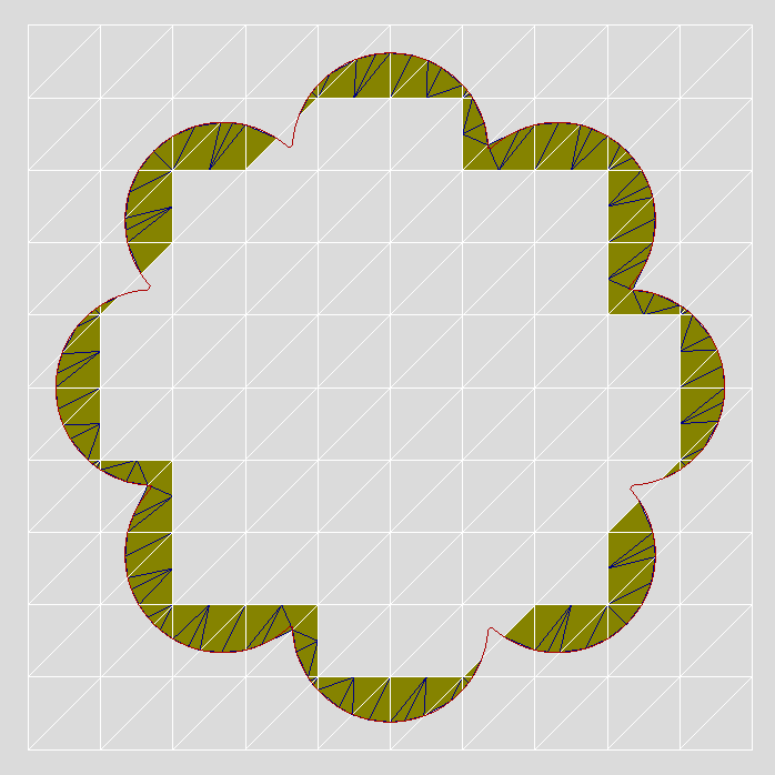
In this subsection we introduce one way to compute the boundary correction error e~Ωsubscriptnorm~𝑒Ω\|\nabla\tilde{e}\|_{{\Omega}}. We firstly construct a boundary correction mesh, denoted by 𝒯hbcsuperscriptsubscript𝒯𝑏𝑐{\mathcal{T}}_{h}^{bc}, which is finer than the current mesh 𝒯hsubscript𝒯{\mathcal{T}}_{h} in order to more accurately track the boundary ΩΩ\partial{\Omega}. More precisely, the new mesh is built inside the union of all intersection elements, i.e.,

K𝒯hbcKK𝒯hbK.subscript𝐾superscriptsubscript𝒯𝑏𝑐𝐾subscript𝐾superscriptsubscript𝒯𝑏𝐾\cup_{K\in{\mathcal{T}}_{h}^{bc}}K\subset\cup_{K\in{\mathcal{T}}_{h}^{b}}K.

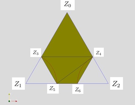
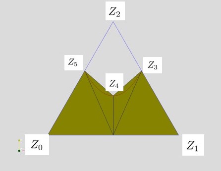
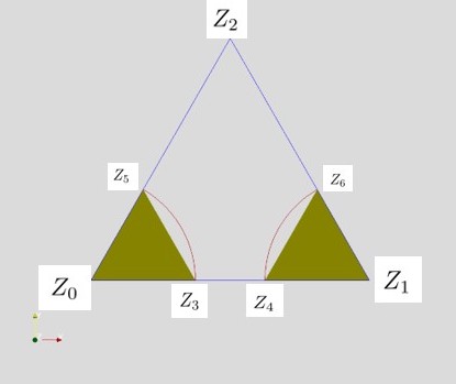
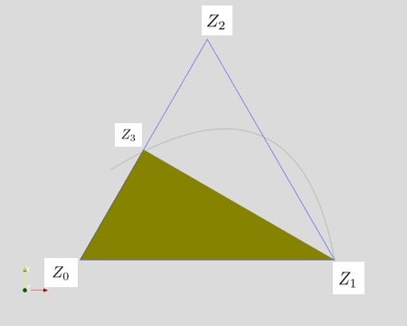
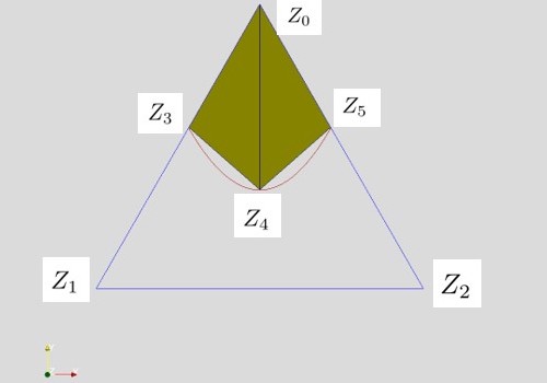
For each element K𝒯𝐾𝒯K\in{\mathcal{T}}, without loss of generality, in two dimensions, we assume that ϕ(z0)ϕ(z1)ϕ(z2)italic-ϕsubscript𝑧0italic-ϕsubscript𝑧1italic-ϕsubscript𝑧2\phi(z_{0})\leq\phi(z_{1})\leq\phi(z_{2}) where zi,i=0,1,2formulae-sequencesubscript𝑧𝑖𝑖012z_{i},i=0,1,2 are vertices of K𝐾K. For each K𝒯hb𝐾superscriptsubscript𝒯𝑏K\in{\mathcal{T}}_{h}^{b} we assume the following must be true: there exists at least one facet in K𝐾K such that the nodes connected to that facet have both positive and negative values, i.e.,

ϕ(z0)<0andϕ(z2)>0.formulae-sequenceitalic-ϕsubscript𝑧00anditalic-ϕsubscript𝑧20\phi(z_{0})<0\quad\mbox{and}\quad\phi(z_{2})>0.

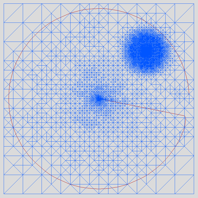
We then further partition the elements in 𝒯hbsuperscriptsubscript𝒯𝑏{\mathcal{T}}_{h}^{b} based on the intersection of the domain and the mesh. The pseudo code for the algorithm is provided in Algorithm 1. An example boundary correction mesh for Example 1 is shown in Fig. 3.
Algorithm 1 Build the boundary correction mesh in two dimensions
  for cell K𝒯hb𝐾superscriptsubscript𝒯𝑏K\in{\mathcal{T}}_{h}^{b}  do
     if  ϕ(z1)>0italic-ϕsubscript𝑧10\phi(z_{1})>0 then
        if  ϕ((z1+z2)/2)0italic-ϕsubscript𝑧1subscript𝑧220\phi((z_{1}+z_{2})/2)\geq 0 then
           Set Type as ’a’
           Find intersection points z3subscript𝑧3z_{3}z5subscript𝑧5z_{5} and form 2 triangles as as shown in Fig. 2a
        else
           Set Type as ’b’
           Find intersection points z3subscript𝑧3z_{3}z6subscript𝑧6z_{6} and form 4 triangles as as in Fig. 2b
        end if
     else if ϕ(z1)<0italic-ϕsubscript𝑧10\phi(z_{1})<0 then
        if  ϕ((z0+z1)/2)<0italic-ϕsubscript𝑧0subscript𝑧120\phi((z_{0}+z_{1})/2)<0 then
           Set Type as ’c’
           Find intersection points z3subscript𝑧3z_{3}z5subscript𝑧5z_{5} and form 4 triangles as as shown in Fig. 2c
        else
           Set Type as ’d’
           Find intersection points z3subscript𝑧3z_{3}z6subscript𝑧6z_{6} and form 2 triangles as as in Fig. 2d
        end if
     else
        Set Type as ’e’
        Find intersection point z3subscript𝑧3z_{3} and form 1 triangle as in in Fig. 2e
     end if
  end for
Refer to caption
(a)
Refer to caption
(b)
Refer to caption
(c)
Refer to caption
(d)
Refer to caption
(e)
Figure 2: Partition of the intersection cell based on the cut of level set.
Refer to caption
Figure 3: An example of the boundary correction mesh for Example 1

With the mesh 𝒯bcsuperscript𝒯𝑏𝑐{\mathcal{T}}^{bc} available, we define e~~𝑒\tilde{e} to be a piecewise linear conforming function with respect to 𝒯hbcsuperscriptsubscript𝒯𝑏𝑐{\mathcal{T}}_{h}^{bc} such that

e~(z)={g(z)uh(z)if zΩ,0otherwise.~𝑒𝑧cases𝑔𝑧subscript𝑢𝑧if 𝑧Ω0otherwise\tilde{e}(z)=\begin{cases}g(z)-u_{h}(z)&\mbox{if }z\in\partial{\Omega},\\[5.69054pt] 0&\mbox{otherwise}.\end{cases}
Remark 5.1.

It is critical that e~~𝑒\tilde{e} is properly designed so that the boundary correction does not over-estimate the error due to the underresolved geometry. In our construction, it is easy to see that e~=g~uh~𝑒~𝑔subscript𝑢\tilde{e}=\tilde{g}-u_{h} on ΩΩ\partial{\Omega} where g~~𝑔\tilde{g} is the nodal interpolation of g𝑔g with respect to 𝒯hbcsuperscriptsubscript𝒯𝑏𝑐{\mathcal{T}}_{h}^{bc} on ΩΩ\partial{\Omega}. Then we have that

g~uh1/2,Ωe~Ωg~uh1/2,Ω.subscriptnorm~𝑔subscript𝑢12Ωsubscriptnorm~𝑒Ωless-than-or-similar-tosubscriptnorm~𝑔subscript𝑢12Ω\|\tilde{g}-u_{h}\|_{1/2,\partial{\Omega}}\leq\|\nabla\tilde{e}\|_{{\Omega}}\lesssim\|\tilde{g}-u_{h}\|_{1/2,\partial{\Omega}}.

The second inequality follows from the equivalence of norms.

5.2 Numerical Examples

Example 5.2.

The level set of the problem has a flower shape (see Fig. 3) that has the following representation:

ϕ=min(ϕ0,ϕ1,,ϕ8)italic-ϕsubscriptitalic-ϕ0subscriptitalic-ϕ1subscriptitalic-ϕ8\phi=\min(\phi_{0},\phi_{1},\cdots,\phi_{8})

with

{ϕ0(x,y)=x2+y2r2,r=2ϕi(x,y)=(xxi)2+(yyi)2ri2,ri=2r(sin(π/8)+cos(π/8))sin(π/8)casessubscriptitalic-ϕ0𝑥𝑦superscript𝑥2superscript𝑦2superscript𝑟2𝑟2subscriptitalic-ϕ𝑖𝑥𝑦superscript𝑥subscript𝑥𝑖2superscript𝑦subscript𝑦𝑖2superscriptsubscript𝑟𝑖2subscript𝑟𝑖2𝑟𝜋8𝜋8𝜋8\begin{cases}\phi_{0}(x,y)=x^{2}+y^{2}-r^{2},&r=2\\ \phi_{i}(x,y)=(x-x_{i})^{2}+(y-y_{i})^{2}-r_{i}^{2},&r_{i}=\sqrt{2}r*(\sin(\pi/8)+\cos(\pi/8))\sin(\pi/8)\end{cases}

for i=1,,8𝑖18i=1,\cdots,8, xi=r(cos(π/8)+sin(π/8))cos(iπ/4)subscript𝑥𝑖𝑟𝜋8𝜋8𝑖𝜋4x_{i}=r(\cos(\pi/8)+\sin(\pi/8))\cos(i*\pi/4) and yi=r(cos(π/8)+sin(π/8))cos(iπ/4)subscript𝑦𝑖𝑟𝜋8𝜋8𝑖𝜋4y_{i}=r(\cos(\pi/8)+\sin(\pi/8))\cos(i*\pi/4). The domain ΩΩ{\Omega} is defined as x2𝑥superscript2x\in\mathbb{R}^{2} such that ϕ(x)0italic-ϕ𝑥0\phi(x)\leq 0. The data are given such that g=0𝑔0g=0 on ΩΩ\partial{\Omega} and

f(x,y)={10if (xx1)2+(yy1)2r12/2.0otherwise.𝑓𝑥𝑦cases10if superscript𝑥subscript𝑥12superscript𝑦subscript𝑦12superscriptsubscript𝑟122missing-subexpression0otherwisemissing-subexpressionf(x,y)=\left\{\begin{array}[]{lll}10&\mbox{if }(x-x_{1})^{2}+(y-y_{1})^{2}\leq r_{1}^{2}/2.\\ 0&\mbox{otherwise}.\end{array}\right.

In the numerical scheme, we take gh=0subscript𝑔0g_{h}=0. With the stopping criteria that the total number of degree of freedoms be not greater than 700070007000, the final meshes obtained without and with adding the boundary correction term are given e~norm~𝑒\|\nabla\tilde{e}\| in Fig. 4a and Fig. 4b, respectively. We observe that slightly more degree of freedoms are added around the concave corners in Fig. 4b. The corresponding convergence performances of each adaptive procedure are given in Fig. 5. We observe that both estimators converge optimally when the mesh become fine enough. Adding the boundary correction term does slightly increases the estimator at the initial stage. However, the weight is diminishing as the mesh gets finer.
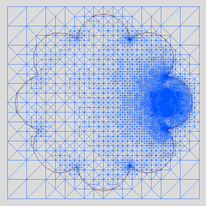
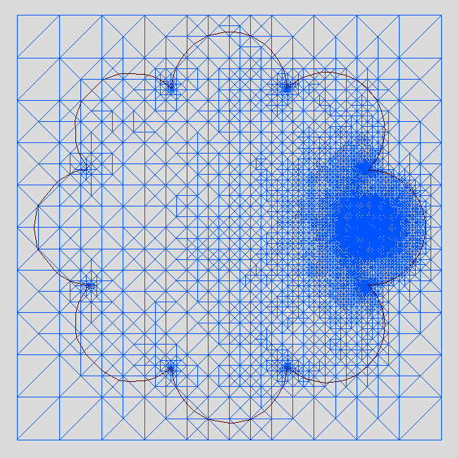
Refer to caption
(a)
Refer to caption
(b)
Figure 4: Final meshes generated without and with e~Ksubscriptnorm~𝑒𝐾\|\nabla\tilde{e}\|_{K}.
Refer to caption
Figure 5: Estimator convergence rate without and with e~norm~𝑒\|\nabla\tilde{e}\|
Example 5.3.

The level set of this problem has the following representation:

ϕ=max(ϕ0,ϕ1,,ϕ8)italic-ϕsubscriptitalic-ϕ0subscriptitalic-ϕ1subscriptitalic-ϕ8\phi=\max(\phi_{0},-\phi_{1},\cdots,-\phi_{8})

with ϕ0subscriptitalic-ϕ0\phi_{0} to ϕ8subscriptitalic-ϕ8\phi_{8} defined the same as in Example 5.2. The datum are chosen such that

f=0andg=y2.formulae-sequence𝑓0and𝑔superscript𝑦2f=0\quad\mbox{and}\quad g=y^{2}.

In the numerical scheme we approximate the boundary by ΩhsubscriptΩ{\Omega}_{h} defined in Eq. 5.1. For the Dirichlet date we take ghsubscript𝑔g_{h} to be the conforming piecewise linear interpolation of g=y2𝑔superscript𝑦2g=y^{2}. With the stopping criteria that the total number of degree of freedoms be not greater than 700070007000, the final meshes obtained without and with adding the boundary correction term e~Ksubscriptnorm~𝑒𝐾\|\nabla\tilde{e}\|_{K} are given in Fig. 6a and Fig. 6b, respectively. The corresponding convergence performance of each adaptive procedure are given in Fig. 7. We observe that in both cases the estimator converges optimally. In Fig. 6b note that there is no more obvious dense refinement comparing to Fig. 6a around the boundary including the corners since in this case the approximation error ggh𝑔subscript𝑔g-g_{h} is of uniform order everywhere.

Refer to caption
(a)
Refer to caption
(b)
Figure 6: Final meshes generated without and with e~Ksubscriptnorm~𝑒𝐾\|\nabla\tilde{e}\|_{K}.
Refer to caption
Figure 7: estimator convergence rate without and with e~norm~𝑒\|\nabla\tilde{e}\|

5.3 Example 3

In this example we consider the reentrant problem whose solution has the following polar representation:

u(r,θ)=rαsin(αθ),𝑢𝑟𝜃superscript𝑟𝛼𝛼𝜃u(r,\theta)=r^{\alpha}\sin(\alpha\theta),

with α=π/ω𝛼𝜋𝜔\alpha=\pi/\omega and ω𝜔\omega being the angle of the reentrant corner. In this example, we test two values for ω𝜔\omega, i.e., 31π/831𝜋831\pi/8 and 63π/1663𝜋1663\pi/16. The stopping criteria is set such that the maximal number of degrees of freedom does not exceed 500050005000. In the numerical scheme we approximate the Dirichlet datum g𝑔g by ghsubscript𝑔g_{h} using conforming piecewise linear interpolation. The final meshes generated without adding the boundary correction error are given in Fig. 8aFig. 8b and with the boundary correction error are given in Fig. 9aFig. 9b. The corresponding convergence rate of estimators are presented in Fig. 10aFig. 10b. We again observe the optimal convergence performance for the estimator and true error in all cases. This indicates that the estimator, with or without the boundary correction error, works equivalently effective for problem even with singularity on the boundary.
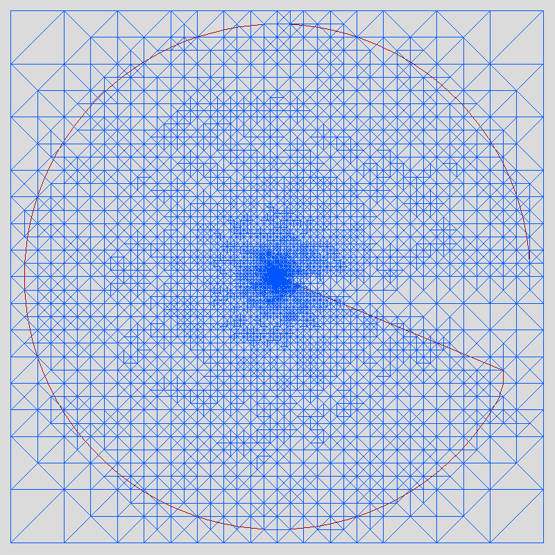
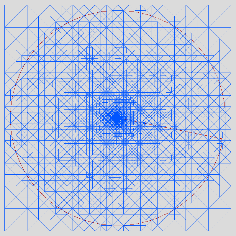
Refer to caption
(a)
Refer to caption
(b)
Figure 8: Final meshes generated without e~Ksubscriptnorm~𝑒𝐾\|\nabla\tilde{e}\|_{K}. Left: ω=31π/8𝜔31𝜋8\omega=31\pi/8. Right: ω=63π/16𝜔63𝜋16\omega=63\pi/16.
Refer to caption
(a)
Refer to caption
(b)
Figure 9: Final meshes generated with e~Ksubscriptnorm~𝑒𝐾\|\nabla\tilde{e}\|_{K}. Left: ω=31π/8𝜔31𝜋8\omega=31\pi/8. Right: ω=63π/16𝜔63𝜋16\omega=63\pi/16.
Refer to caption
(a)
Refer to caption
(b)
Figure 10: Estimator convergence performance without and with e~norm~𝑒\|\nabla\tilde{e}\|. Left: ω=31π/8𝜔31𝜋8\omega=31\pi/8. Right: ω=63π/16𝜔63𝜋16\omega=63\pi/16.

We now test the same procedure but with ghsubscript𝑔g_{h} to be the piecewise constant interpolation of g𝑔g for w=31π/16𝑤31𝜋16w=31\pi/16. From the final meshes generated in Fig. 11a and Fig. 11b we observe that more degree of freedoms are added around the boundary in both cases due to the poorer approximation of the boundary data. The estimators, however, still converges optimally in both cases when the meshes are fine enough.
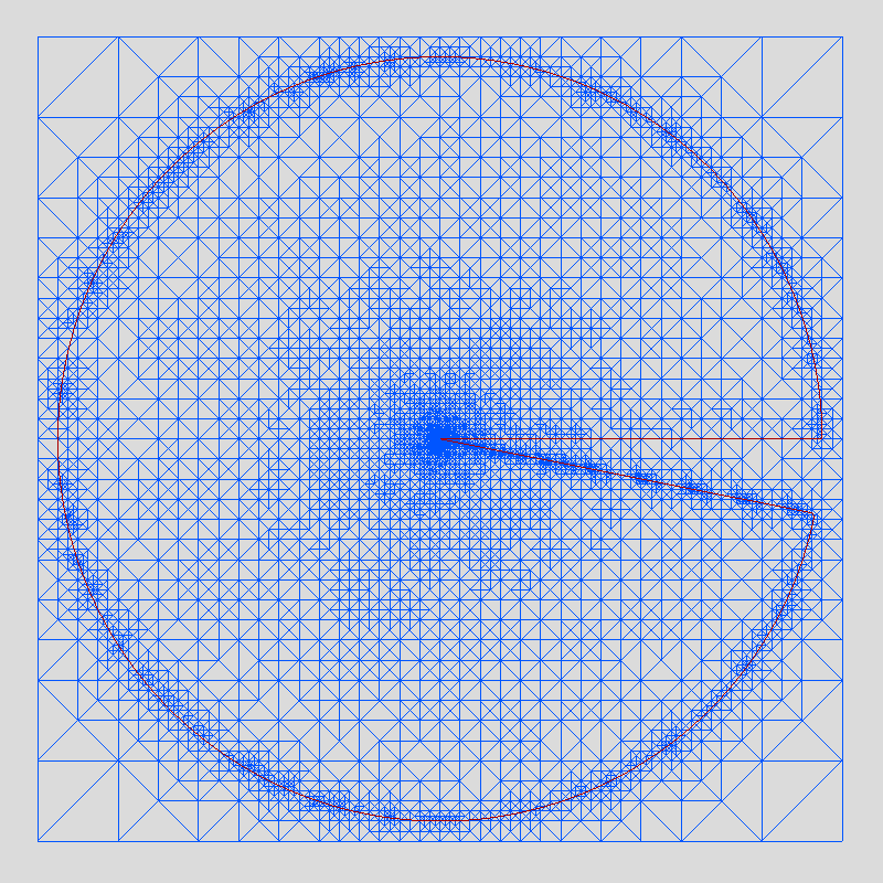
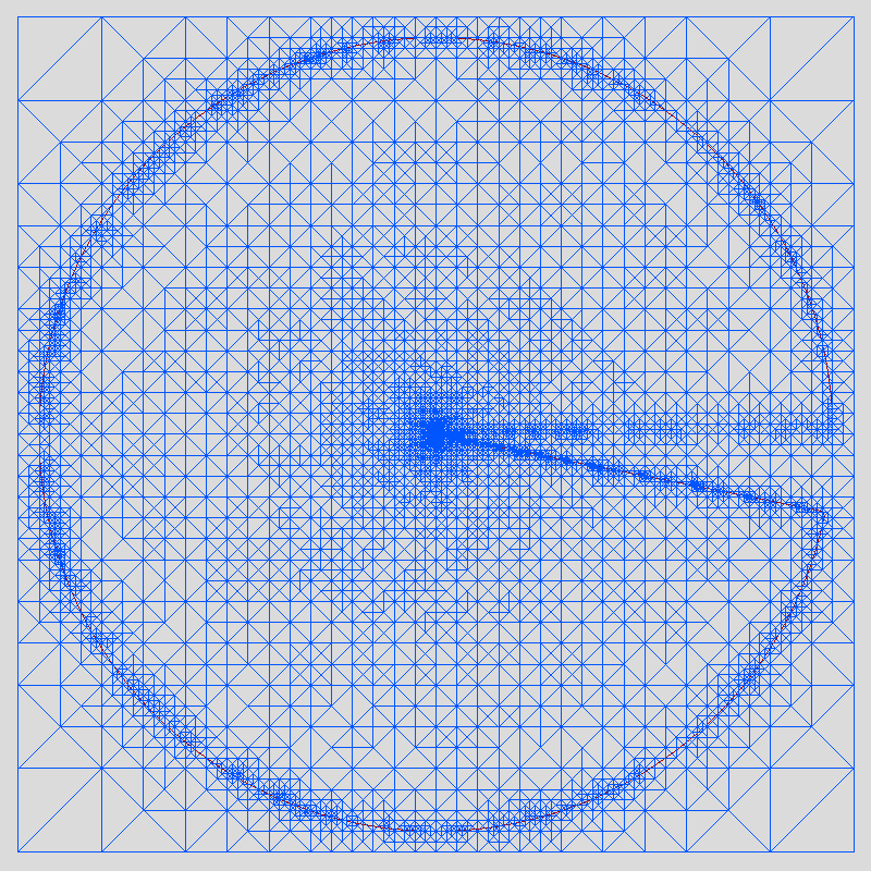
Refer to caption
(a)
Refer to caption
(b)
Figure 11: Final meshes without and with e~norm~𝑒\|\nabla\tilde{e}\|.
Refer to caption
Figure 12: Convergence performance for estimator without and with boundary correction.

5.4 Example 4

In this example, we consider the problem that has the following representation:

u(x,y)=rαsin(αθ)+exp(100((x0.5)2+(y0.5)2))𝑢𝑥𝑦superscript𝑟𝛼𝛼𝜃𝑒𝑥𝑝100superscript𝑥0.52superscript𝑦0.52u(x,y)=r^{\alpha}\sin(\alpha\theta)+exp(100*((x-0.5)^{2}+(y-0.5)^{2}))

with r=x2+y2𝑟superscript𝑥2superscript𝑦2r=\sqrt{x^{2}+y^{2}}, θ=tan1(y/x)𝜃superscript1𝑦𝑥\theta=\tan^{-1}(y/x), α=π/ω𝛼𝜋𝜔\alpha=\pi/\omega and ω=31π/16𝜔31𝜋16\omega=31\pi/16. This problem has multiple singularities with one reentrant corner at (0.0)0.0(0.0) and one peak at (0.5,0.5)0.50.5(0.5,0.5). In the numerical scheme, ghsubscript𝑔g_{h} and fhsubscript𝑓f_{h} are taken as the linear nodal interpolation of g𝑔g and f𝑓f, respectively. The stopping criteria is set to not exceed the maximal refinement step of 505050 and the maximal number of degrees of freedom of 750075007500. The final meshes are given in Fig. 13a and Fig. 13b and their corresponding convergence performance are presented in Fig. 14.
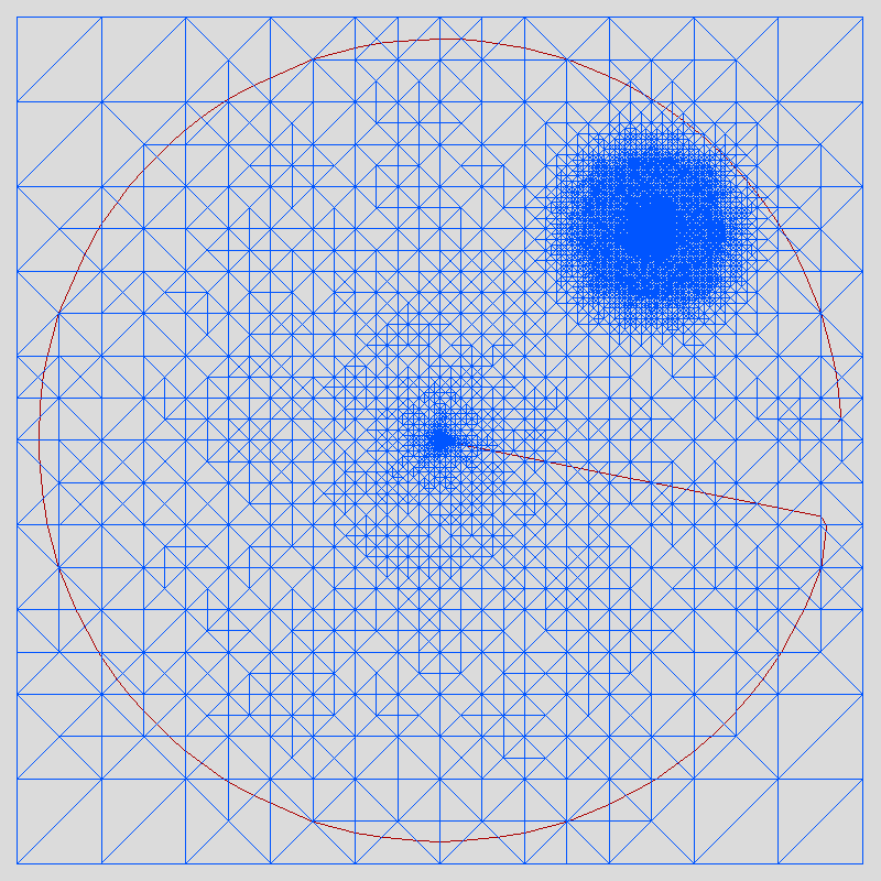
Refer to caption
(a)
Refer to caption
(b)
Figure 13: Final meshes generated without (left) and with (right) e~Ksubscriptnorm~𝑒𝐾\|\nabla\tilde{e}\|_{K}.
Refer to caption
Figure 14: Convergence performance for estimator without and with e~norm~𝑒\|\nabla\tilde{e}\|.

This example shows that the algorithm works also effectively when multiple singularities occurs, no matter the singularity happens on the boundary or inside the domain.

Acknowledgement

EB and CH were supported by EPSRC, UK, Grant No.
EP/P01576X/1. ML was supported by the Swedish Foundation for Strategic Research Grant No. AM13-0029, the Swedish Research Council Grants No. 2017-03911, and the Swedish strategic research programme eSSENCE.

References

  • Ainsworth & Oden, (2011) Ainsworth, Mark, & Oden, J Tinsley. 2011. A posteriori error estimation in finite element analysis. Vol. 37. John Wiley & Sons.
  • Ainsworth & Rankin, (2017) Ainsworth, Mark, & Rankin, Richard. 2017. Computable error bounds for finite element approximation on nonpolygonal domains. IMA Journal of Numerical Analysis, 37(2), 604–645.
  • Barrett & Elliott, (1984) Barrett, John W., & Elliott, Charles M. 1984. A finite-element method for solving elliptic equations with Neumann data on a curved boundary using unfitted meshes. IMA J. Numer. Anal., 4(3), 309–325.
  • Becker et al. , (2011) Becker, Roland, Burman, Erik, & Hansbo, Peter. 2011. A hierarchical NXFEM for fictitious domain simulations. Internat. J. Numer. Methods Engrg., 86(4-5), 549–559.
  • Bernland et al. , (2018) Bernland, A., Wadbro, E., & Berggren, M. 2018. Acoustic shape optimization using cut finite elements. Internat. J. Numer. Methods Engrg., 113(3), 432–449.
  • Bertoluzza et al. , (2005) Bertoluzza, S., Ismail, M., & Maury, B. 2005. The fat boundary method: semi-discrete scheme and some numerical experiments. Pages 513–520 of: Domain decomposition methods in science and engineering. Lect. Notes Comput. Sci. Eng., vol. 40. Springer, Berlin.
  • Boiveau et al. , (2018) Boiveau, T., Burman, E., Claus, S., & Larson, M. 2018. Fictitious domain method with boundary value correction using penalty-free Nitsche method. J. Numer. Math., 26(2), 77–95.
  • Bramble & King, (1994) Bramble, James H., & King, J. Thomas. 1994. A robust finite element method for nonhomogeneous Dirichlet problems in domains with curved boundaries. Math. Comp., 63(207), 1–17.
  • Bui et al. , (2019) Bui, H. P., Tomar, S., & Bordas, S. P. A. 2019. Corotational cut finite element method for real-time surgical simulation: application to needle insertion simulation. Comput. Methods Appl. Mech. Engrg., 345, 183–211.
  • Burman, (2010) Burman, E. 2010. Ghost penalty. C. R. Math. Acad. Sci. Paris, 348(21-22), 1217–1220.
  • Burman & Ern, (2019) Burman, E., & Ern, A. 2019. A cut cell hybrid high-order method for elliptic problems with curved boundaries. Pages 173–181 of: European Conference on Numerical Mathematics and Advanced Applications, ENUMATH 2017; Voss; Norway. Lecture Notes in Computational Science and Engineering, vol. 126.
  • Burman & Hansbo, (2010) Burman, E., & Hansbo, P. 2010. Fictitious domain finite element methods using cut elements: I. A stabilized Lagrange multiplier method. Comput. Methods Appl. Mech. Engrg., 199(41-44), 2680–2686.
  • Burman & Hansbo, (2012) Burman, E., & Hansbo, P. 2012. Fictitious domain finite element methods using cut elements: II. A stabilized Nitsche method. Appl. Numer. Math., 62(4), 328–341.
  • Burman & Hansbo, (2014) Burman, E., & Hansbo, P. 2014. Fictitious domain methods using cut elements: III. A stabilized Nitsche method for Stokes’ problem. ESAIM Math. Model. Numer. Anal., 48(3), 859–874.
  • Burman et al. , (2015a) Burman, E., Claus, S., & Massing, A. 2015a. A stabilized cut finite element method for the three field Stokes problem. SIAM J. Sci. Comput., 37(4), A1705–A1726.
  • Burman et al. , (2017) Burman, E., Elfverson, D., Hansbo, P., Larson, M. G., & Larsson, K. 2017. A cut finite element method for the Bernoulli free boundary value problem. Comput. Methods Appl. Mech. Engrg., 317, 598–618.
  • Burman et al. , (2018a) Burman, E., Hansbo, P., & Larson, M. G. 2018a. A cut finite element method with boundary value correction. Math. Comp., 87(310), 633–657.
  • Burman et al. , (2018b) Burman, E., Elfverson, D., Hansbo, P., Larson, M. G., & Larsson, K. 2018b. Shape optimization using the cut finite element method. Comput. Methods Appl. Mech. Engrg., 328, 242–261.
  • Burman et al. , (2015b) Burman, Erik, Claus, Susanne, Hansbo, Peter, Larson, Mats G., & Massing, André. 2015b. CutFEM: discretizing geometry and partial differential equations. Internat. J. Numer. Methods Engrg., 104(7), 472–501.
  • Cai et al. , (2017) Cai, Zhiqiang, He, Cuiyu, & Zhang, Shun. 2017. Residual-based a posteriori error estimate for interface problems: Nonconforming linear elements. Mathematics of Computation, 86(304), 617–636.
  • Di Pietro & Ern, (2012) Di Pietro, D. A., & Ern, A. 2012. Mathematical aspects of discontinuous Galerkin methods. Mathématiques & Applications (Berlin) [Mathematics & Applications], vol. 69. Springer, Heidelberg.
  • Dörfler & Rumpf, (1998) Dörfler, Willy, & Rumpf, Martin. 1998. An adaptive strategy for elliptic problems including a posteriori controlled boundary approximation. Mathematics of Computation of the American Mathematical Society, 67(224), 1361–1382.
  • Elfverson et al. , (2018) Elfverson, D., Larson, M. G., & Larsson, K. 2018. CutIGA with Basis Function Removal. arXiv e-prints, Jan.
  • Embar et al. , (2010) Embar, Anand, Dolbow, John, & Harari, Isaac. 2010. Imposing Dirichlet boundary conditions with Nitsche’s method and spline-based finite elements. Internat. J. Numer. Methods Engrg., 83(7), 877–898.
  • Glowinski & Pan, (1992) Glowinski, R., & Pan, T.-W. 1992. Error estimates for fictitious domain/penalty/finite element methods. Calcolo, 29(1-2), 125–141 (1993).
  • Grisvard, (2011) Grisvard, Pierre. 2011. Elliptic problems in nonsmooth domains. Classics in Applied Mathematics, vol. 69. Society for Industrial and Applied Mathematics (SIAM), Philadelphia, PA. Reprint of the 1985 original [ MR0775683], With a foreword by Susanne C. Brenner.
  • Gürkan & Massing, (2019) Gürkan, Ceren, & Massing, André. 2019. A stabilized cut discontinuous Galerkin framework for elliptic boundary value and interface problems. Computer Methods in Applied Mechanics and Engineering, 348, 466–499.
  • Guzmán & Olshanskii, (2018) Guzmán, J., & Olshanskii, M. 2018. Inf-sup stability of geometrically unfitted Stokes finite elements. Math. Comp., 87(313), 2091–2112.
  • Hansbo & Hansbo, (2002) Hansbo, Anita, & Hansbo, Peter. 2002. An unfitted finite element method, based on Nitsche’s method, for elliptic interface problems. Comput. Methods Appl. Mech. Engrg., 191(47-48), 5537–5552.
  • Hansbo et al. , (2015) Hansbo, P., Larson, M. G., & Zahedi, S. 2015. Characteristic cut finite element methods for convection-diffusion problems on time dependent surfaces. Comput. Methods Appl. Mech. Engrg., 293, 431–461.
  • Hansbo et al. , (2017) Hansbo, Peter, Larson, Mats G, & Larsson, Karl. 2017. Cut finite element methods for linear elasticity problems. Pages 25–63 of: Geometrically Unfitted Finite Element Methods and Applications. Springer.
  • Haslinger & Renard, (2009) Haslinger, J., & Renard, Y. 2009. A new fictitious domain approach inspired by the extended finite element method. SIAM J. Numer. Anal., 47(2), 1474–1499.
  • Johansson & Larson, (2013) Johansson, A., & Larson, M. G. 2013. A High Order Discontinuous Galerkin Nitsche Method for Elliptic Problems with Fictitious Boundary. Numer. Math., 123(4), 607–628.
  • Jonsson et al. , (2019) Jonsson, Tobias, Larson, Mats G, & Larsson, Karl. 2019. Graded parametric CutFEM and CutIGA for elliptic boundary value problems in domains with corners. Computer Methods in Applied Mechanics and Engineering.
  • Lehrenfeld, (2017) Lehrenfeld, C. 2017. A higher order isoparametric fictitious domain method for level set domains. Pages 65–92 of: Geometrically Unfitted Finite Element Methods and Applications. Lect. Notes Comput. Sci. Eng., vol. 121. Springer, Cham.
  • Massing et al. , (2014a) Massing, A., Larson, M. G., Logg, A., & Rognes, M. E. 2014a. A stabilized Nitsche fictitious domain method for the Stokes problem. J. Sci. Comput., 61(3), 604–628.
  • Massing et al. , (2018) Massing, A., Schott, B., & Wall, W. A. 2018. A stabilized Nitsche cut finite element method for the Oseen problem. Comput. Methods Appl. Mech. Engrg., 328, 262–300.
  • Massing et al. , (2014b) Massing, André, Larson, Mats G., Logg, Anders, & Rognes, Marie E. 2014b. A stabilized Nitsche fictitious domain method for the Stokes problem. J. Sci. Comput., 61(3), 604–628.
  • Nitsche, (1971) Nitsche, J. 1971. Über ein Variationsprinzip zur Lösung von Dirichlet-Problemen bei Verwendung von Teilräumen, die keinen Randbedingungen unterworfen sind. Abh. Math. Sem. Univ. Hamburg, 36, 9–15. Collection of articles dedicated to Lothar Collatz on his sixtieth birthday.
  • Schott & Wall, (2014) Schott, B., & Wall, W. A. 2014. A new face-oriented stabilized XFEM approach for 2D and 3D incompressible Navier-Stokes equations. Comput. Methods Appl. Mech. Engrg., 276, 233–265.
  • Schott et al. , (2016) Schott, B., Shahmiri, S., Kruse, R., & Wall, W. A. 2016. A stabilized Nitsche-type extended embedding mesh approach for 3D low- and high-Reynolds-number flows. Internat. J. Numer. Methods Fluids, 82(6), 289–315.
  • Scott & Zhang, (1990) Scott, L Ridgway, & Zhang, Shangyou. 1990. Finite element interpolation of nonsmooth functions satisfying boundary conditions. Mathematics of Computation, 54(190), 483–493.
  • Swift, (2018) Swift, L. 2018. Geometrically unfitted finite element methods for the Helmholtz equation. Ph.D. thesis, University College London.
  • Verfürth, (1994) Verfürth, Rüdiger. 1994. A posteriori error estimation and adaptive mesh-refinement techniques. Journal of Computational and Applied Mathematics, 50(1-3), 67–83.
  • Winter et al. , (2018) Winter, M., Schott, B., Massing, A., & Wall, W. A. 2018. A Nitsche cut finite element method for the Oseen problem with general Navier boundary conditions. Comput. Methods Appl. Mech. Engrg., 330, 220–252.