Structure Formation with Two Periods of Inflation:
Beyond PLaIn CDM
Kari Enqvist, Till Sawala, and Tomo Takahashi
a
Department of Physics and
Helsinki Institute of Physics, FIN-00014,
University of Helsinki, Finland
b
Department of Physics, Saga University, Saga 840-8502, Japan
We discuss structure formation in models with a spectator field in small-field inflation which accommodate a secondary period of inflation. In such models, subgalactic scale primordial fluctuations can be much suppressed in comparison to the usual power-law CDM model while the large scale fluctuations remain consistent with current observations. We discuss how a secondary inflationary epoch may give rise to observable features in the small scale power spectrum and hence be tested by the structures in the Local Universe.
1 Introduction
The standard “Lambda Cold Dark Matter” (hereafter plain CDM, or CDM with POwer LAw Inflation#1#1#1 Here “power law” indicates that primordial power spectrum is of a “power-law” form. Do not confuse with power law inflation model in which the inflaton potential is given by an exponential function. ) model of cosmology is founded on three key assumptions: firstly, that the Universe contains, in addition to baryonic matter, a collisionless, “cold” dark matter component that accounts for of the matter density; secondly, that the expansion of the Universe is described by the Friedmann equations with a cosmological constant term, , and, thirdly, the implicit assumption that structure formation has its origin in the primordial perturbations seeded by inflation.
The plain CDM model has successfully predicted structure formation over many epochs and orders of magnitude, from the structures observed in the Cosmic Microwave Background (CMB) at to the sizes and distributions of clusters and galaxies at much later time. However, tensions between the CMB and measurements on small scales have also been reported. These have either been attributed to poorly understood systematic effects in various data sets, or interpreted as an indication of new physics.
On small scales, predictions for structure formation concern the abundance and internal structure of low mass dark matter halos in the Local Universe. Here, observations of the Milky Way and Andromeda satellite populations in particular, appear to be in disagreement with N-body simulations based on the plain CDM model.
This tension is twofold. The “missing satellites” problem [1, 2] refers to the apparent paucity of luminous satellite galaxies compared to the large number of dark matter substructures predicted in plain CDM. While processes including supernova feedback (e.g. [3]), and cosmic reionisation (e.g. [4]) are expected to reduce the number of observed satellite galaxies, the apparent excess of substructures in the plain CDM is not limited to the lowest mass scales: simulations also predict the presence of subhalos so massive that they should not be affected by reionisation (and hence deemed “too big to fail”, [5]), but whose internal structure seems incompatible with that of the brightest observed satellites.
Recent hydrodynamic simulations have shown that, when baryonic effects are included, the observed Local Group satellite populations can be reproduced in CDM (e.g. [6]), but only if the Local Group mass is , at the lower end of the observational limits [7]. It has also been shown that, if the CDM assumption of the plain CDM model is relaxed, simulations of warm dark matter [8, 9] and photon-coupled dark matter [10], which both reduce the small-scale power after decoupling, give a better agreement to satellite kinematics than the equivalent plain CDM models. Conversely, observed structures in the Lyman- forest [11, 12], and the abundance of Milky Way satellites [13] also provide upper limits for any reduction of small scale power relative to plain CDM.
Warm dark matter models prevent the hierarchical formation of structures below the free-streaming scale (e.g. [15]), but above that, the abundance of structures relative to CDM differs significantly over only a narrow range. Consequently, within current limits, WDM effects are testable only at or below the scale of ultra-faint dwarf galaxies [8]. This gives WDM models limited predictive power. Furthermore, the motivation for the required WDM particle appears somewhat ad-hoc. Another, perhaps more attractive possibility, is to modify the power spectrum of primordial perturbations. The modification should be such that it persists over orders of magnitude; hence e.g. local features in the inflation potential are unlikely to do the job.
Instead, here we propose a unified description of structure formation that relies on two periods of inflation and accounts both for the power on CMB scales and for the apparent suppression of power on subgalactic scales.
There exist models for two periods of inflation making use e.g. of a suitably arranged inflaton potential with an intervening phase transition [16, 17]#2#2#2 It has been argued that the CMB spectral distortion would be useful to differentiate models with a small-scale suppression of the matter power spectrum due late-time effects (such as different dark matter properties) from those caused by a modification of the primordial power spectrum [18]. .
In this paper we consider a model where the inflaton field, giving rise to a slow roll inflation, is complemented by another scalar field, which is dynamically irrelevant during the first period of inflation. Such a scalar is called a spectator field. We know that spectator fields exist: the Higgs field is one example (see, e.g., [19, 20, 21] for fluctuations of the mean Higgs field during inflation), barring the possibility that the Higgs field itself is the inflaton. Another, much studied spectator field is the curvaton [22, 23, 24] which imprints the perturbations it receives during inflation on radiation and matter after inflation#3#3#3Another example would be the modulated reheating model [25, 26]. Rather than the inflaton, the curvaton could then be the origin of the whole of the observed spectrum of perturbations.
Here we do not assume that the spectator field contributes to the primordial perturbation in a significant manner. Instead, we assume that it gives rise to second period of inflation, which happens under the conditions to be discussed below. Such a second period of inflation affects the power spectrum both on the CMB scales as well as on subgalactic scales. In this paper we shall discuss a model with two periods of inflation that yields the desired suppression at small scales while remaining in agreement with the observed properties of the CMB power spectrum, making it possible to address the apparent shortfalls of the plain CDM model at small scales in completely different, and astrophysically decoupled regimes. Such agreement, however, makes certain demands on the inflaton model; not all inflationary potentials are consistent with two inflationary periods. We will also demonstrate that for our working example, the fact that some subgalactic structure has actually been observed gives rise to a lower limit on the number of -folds of the first inflationary period.
This paper is organized as follows. In Section 2, we briefly introduce the general concept of a spectator field, and in Sections 2.1 and 2.2 we describe the background evolution and perturbation, respectively. In Section 3, we introduce a concrete inflation model. In Section 4 we discuss the predictions for small scale power. We conclude with a summary in Section 5.
2 Spectator fields
Fields whose energy densities during inflation are irrelevant for the expansion rate of the Universe are called spectators. If they are light, both their mean field values and the field perturbations will be subject to inflaton-driven inflationary expansion. At the onset of inflation the spectator energy density is subdominant. The spectator field is assumed to begin to oscillate during the radiation-dominated period after the inflaton field has decayed (or during the period dominated by the oscillations of the inflaton). Its energy density depends on the initial spectator field value , as well as on the exact form of the spectator potential. During inflation, the mean spectator field is subject to fluctuations and in a given inflationary patch is one realization of the probability distribution, which is determined by the Fokker-Planck equation#4#4#4Assuming slow-roll inflation, as will be done here. as was first pointed out by Starobinsky [27] (for a discussion in the context of spectators, see e.g [28, 29]).
At the end of inflation, the spectator square-mean-field has a value , which serves as the initial spectator field value for its subsequent evolution. As a consequence of its stochastic evolution during inflation, it may have a value greater than the Planck mass . If inflation lasts long enough, the probability distribution for the initial curvaton field equilibrates; otherwise there will be a dependence on the curvaton field value before the onset of inflation (however, equilibration is not automatic; for a recent discussion on the fluctuations of spectator fields, see [29]). In any case, if , the spectator may end up dominating the Universe even before it starts to oscillate. This happens, provided that the spectator is still slowly rolling down its potential, whence a period of secondary inflation can ensue[30, 31, 32, 33]. Thus, very crudely, first there is a period of inflation driven by the “usual” inflaton field; then the inflaton decays; after a while, the energy density of the slowly rolling spectator becomes dominant and generates a second period of inflation, which ends when the spectator decays. This scenario, which we investigate in the present paper, has some very interesting consequences, in particular for the spectrum of perturbations at small scales. As we will discuss, these consequences will also depend on the details of the slow roll inflation model.
Depending on the duration of the secondary inflation driven by the spectator, the current observable scales (such as CMB) may have exited the horizon either during the primary slow roll inflationary phase or during the secondary, spectator-driven phase. In the standard case with no inflating spectator, the required number of -folds is usually taken to be -folds. However, depending on the duration of the secondary inflationary phase, we may tolerate primary -folds as low as . In such a case, the predictions for the primordial power spectrum can be drastically modified.
The spectator modifies the spectrum of perturbations already at the CMB scales. Because the first phase of inflation ends early, the modes corresponding to the CMB scales which exited the horizon closer to the end of the inflaton period, at which the inflaton starts to move faster, even if it is still slowly rolling. As a result, there will be a large running of the spectral index, which may also significantly modify the predictions for astrophysical scales.
2.1 Background evolution
Before describing primordial density fluctuations, let us first look at the background evolution when a primary inflationary period is followed by a secondary period driven by a spectator.
If the spectator is to drive a secondary phase of inflation, it has to dominate the Universe before it begins to oscillate. This condition is given by
| (2.1) |
where is the spectator field value set during the first inflationary phase, is the radiation energy density at the beginning of the spectator oscillation and is the potential of . The spectator oscillation starts when , where is the mass of the spectator. Throughout this paper we will assume that the spectator potential reads simply
| (2.2) |
whence the above condition can be rewritten as
| (2.3) |
where is the reduced Planck mass. From (2.3) we obtain the condition for the spectator-driven secondary inflation as
| (2.4) |
The mass and the initial field value of the spectator are generally assumed to be model parameters. If one has a long period of initial inflaton-driven inflation so that the curvaton reaches the Fokker-Planck equilibrium distribution, a typical value of the amplitude of the spectator field is given by [28, 29]
| (2.5) |
with being the Hubble rate during inflation, in which de-Sitter (a constant ) background is assumed. Although whether this distribution can be reached or not depends on inflation models, when an inflation model with a potential of the plateau type is adopted, the spectator field can obtain the de-Sitter equilibrium [29]. On the other hand, for the case of large-field inflation models, the equilibrium solution would not be reached although the spectator can still acquire a super-Planckian amplitude in the regime of an eternal inflation [29].
Once the equilibrium value is reached, by using the fact that the inflationary Hubble scale is directly related to the slow-roll parameter as #5#5#5 Here we assume that primordial perturbations are generated only from an inflaton. , the above expression can be recast as
| (2.6) |
from which one can see that the amplitude of a spectator field can be as large as for some set of parameters. As noted before, when , the spectator can give rise to the secondary inflation. From Eq. (2.6) we can see that such a scenario may in fact be generic, given the stochastic behaviour of during the primary inflation and the relation (2.5). Even if the equilibrium value is not reached, the initial value of the spectator can be regarded as a model parameter, which does not prohibit of having a value as large as . Therefore a scenario with a second period of inflation driven by a spectator could be realized in a broad class of model.
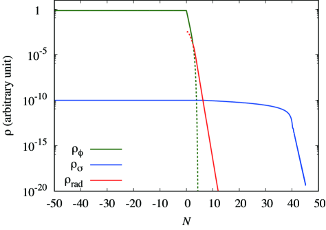
In Fig. 1, we show a typical thermal history in the scenario with two periods of inflation, the second driven by a spectator. We display the evolution of energy densities of the inflaton, the spectator and radiation, denoted as and , respectively. In the following, we focus on the case where the spectator gives a second inflationary period after the CMB scales have already exited the horizon close to the end of the first period of inflation so that the small scale fluctuations are suppressed.
2.2 Density perturbation
In a scenario where a spectator field is present, both the inflaton and the spectator may contribute to the primordial fluctuations (in which case the spectator is a curvaton) for the mode which exited the horizon during the first inflationary epoch driven by the inflaton. For the modes which exited the horizon during the second inflationary epoch driven by a spectator, primordial fluctuations are sourced from the spectator alone. Although we consider a case where fluctuations from a spectator field can be neglected in the next section, here we also discuss the curvature perturbation generated by a spectator in order to clarify in what case spectator fluctuations can be neglected. Here we consider the curvaton type model.
As mentioned above, for modes which exited the horizon during the first inflationary period generated by the inflaton field, the curvature perturbation is in general given by the sum of two contributions#6#6#6 For a general discussion on a scenario where the inflaton and the spectator can both contribute to the curvature perturbation, we refer the readers to [30, 34, 31, 35, 32, 36, 37, 38, 39, 40] for the curvaton model and [41] for modulated reheating scenario. :
| (2.7) |
where and are respectively the curvature perturbations generated from the inflaton and the spectator (which in this case should be called the curvaton). A subscript indicates that the perturbations correspond to modes which exited the horizon during the first inflation. The inflaton part can be written as
| (2.8) |
in which and are the potential for the inflaton and its derivative with respect to the inflaton field and the fluctuation of the inflaton is given by . Therefore the primordial power spectrum sourced by inflaton fluctuations is given by
| (2.9) |
For the curvaton part, here we give the expression for the case where the curvaton drives the secondary inflation since we mainly consider this kind of scenario in this paper. By adopting the formalism [42, 43, 44], the curvature perturbation generated from the spectator is given by where is the number of -folds from the epoch when the mode exited the horizon to that at the decay of the curvaton. However, in the case where the second inflation is driven by a spectator, the -dependence of comes from the period during the second inflation. The number of -folds during such a secondary inflation is given by [32]
| (2.10) |
where and are the potential of the curvaton and the derivative with respect to , respectively. Here is the value of at the end of the second inflation. Here we adopt the potential (2.2) and hence is given by
| (2.11) |
from which we can obtain [32]
| (2.12) |
with . The condition where fluctuations from the curvaton are negligible can be written as
| (2.13) |
from which one can see that, even when , fluctuations from a spectator can be negligible if small-field inflation models with very small are assumed.
On small scales where modes exited the horizon during the second inflation driven by a spectator, the curvature perturbation is given by the same expression as for the ones generated from the inflaton during the first inflationary period. Hence one can write
| (2.14) |
with being determined by the Hubble parameter during the second inflation . The mass for the spectator should be much smaller than since otherwise the spectator field plays the role of the inflaton, and hence . Therefore primordial fluctuations on small scales would be much smaller than those generated on large scales from the inflaton fluctuations. This gives an effective cutoff in the power spectrum at some scale, which may have interesting implications for small scale structure while CMB scale is not affected. In the next section, we assume the above kind of scenario in an inflaton model with very small .
3 A concrete model and power spectrum
To compute the power spectrum in this kind of scenario explicitly, we also need to specify the inflaton model. Although many inflationary potentials would be admissible to have a model with a consistent and with current observations, here let us consider the following inflaton model, which is a hybrid inflation with a fractional power whose potential is given by
| (3.15) |
where represents the scale of inflation, which is determined by the normalization condition. Here and are model parameters which will be chosen to give the spectral index consistent with current observations. This type of inflation model is also called “valley hybrid inflation (VHI)” in [45].
The slow-roll parameters in this model are given by
| (3.16) |
where we have defined
| (3.17) |
The number of -folds counted from the end of the first inflationary period is given by
| (3.18) |
Now we consider the case of , which corresponds to , however when we assume , is very close to unity. As described below, if the secondary inflation is driven by a spectator field, can be much reduced, which can lead to a value consistent with current observations (). To consider the situation where the spectator does not contribute to primordial fluctuations but only affects the background dynamics, we require a very small value for as shown in the previous section. To realize this, here we assume a large value for i.e. (for concreteness, we assume in the following). We also need a very small . In this case, the approximate number of -folds is
| (3.19) |
When and , we have #7#7#7 With the value of the model parameters assumed here, we have very small as . , which, with the help of Eq. (3.16) gives the spectral index as
| (3.20) |
If we take , the spectral index is for , which is outside the region allowed by Planck. However, when the curvaton generates a secondary inflation to make much smaller, say , the spectral index becomes , which gives a good fit to the current Planck data.
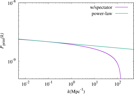
In Fig. 2, we show the primordial power spectrum (left) and matter power spectrum (right) for the case of in the VHI inflation model, in which the CMB scale corresponds to the modes exited the horizon at during the first inflationary period. For comparison, the power spectrum is also shown for the case where the power-law form is assumed. As can be understood from Eq. (2.8) in the previous section, the curvature perturbations are generally suppressed on small scales where the modes exit the horizon close to the end of inflation, since is getting larger. As discussed in the previous section, in our scenario, small scale fluctuations of the modes which exited the horizon during the second inflationary period are much smaller that those on larger scales generated during the first inflation. Therefore we can see the cutoff of the primordial power spectrum at around which corresponds to the mode which exited the horizon at the end of the first inflationary period. This can be clearly seen in the left panel of Fig. 2, which gives interesting implications to the tension between CMB and subgalactic scales.
To discuss the implication of our scenario for the small scale structure, we calculate the matter power spectrum in the present Universe. In the right panel of Fig 2, we plot the matter power spectrum at for the same model. To calculate the matter power spectrum, we need to incorporate the effects of the evolution of fluctuations after the modes crossed the horizon. In particular, there are two periods of inflation in our model, which is quite similar to the case of thermal inflation where a mini-inflation occurs after the first inflation driven by the inflaton. The transfer function in thermal inflation model has been investigated in [46], where an analytic formula is provided as
| (3.21) |
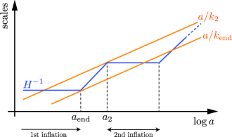
Here is the wave number which corresponds to the mode which “touched” the horizon at the start of the second inflation ( is denoted as in [46]). The above transfer function exhibits oscillatory damping at scales smaller than which can be related to , the mode which exited the horizon at the end of the first inflation once we fix the background evolution. Since holds at the time of the horizon crossing, one has
| (3.22) |
where a subscript “2” denotes that the quantity is evaluated at the beginning of the second inflation. In Fig. 3, a schematic figure of the horizon crossings for two characteristic scales and is shown. Assuming that the Universe is oscillation-dominated#8#8#8 Depending on the decay rate of the inflaton, the Universe may have become radiation-dominated before the second inflation starts. However, we assume that oscillation-domination in the following. , in which , we obtain
| (3.23) |
Assuming that the Hubble parameter during inflation does not change much and hence we can approximate the Hubble parameter at the end of the first inflation as as mentioned just above Eq. (2.6). The Hubble rate at the beginning of the second inflation can be written as , from which one has
| (3.24) |
For the case of depicted in Fig. 2, the damping scale corresponding to the end of the first inflation is given by , and hence the damping scale in the transfer function is estimated as .
In the large and small scale limits ( and , respectively), Eq. (3) gives the transfer function [46]
| (3.25) |
where . Cosmological N-body simulations with the above transfer function have been studied by [47] for the thermal inflation model. It should be noted that, in our model, the primordial power spectrum also gives the suppression on small scales due to the mechanism discussed in the previous section, and hence the power spectrum after the second inflation is given by
| (3.26) |
where is given by Eq. (3) and can be calculated by Eq. (2.9) when only the inflaton contributes to the primordial curvature perturbation.
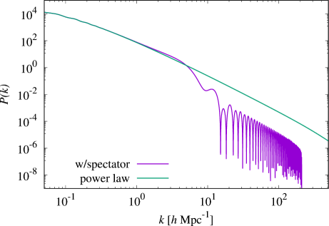
We input to the public code CAMB [48] to obtain the matter power spectrum at late time, which is shown in the right panel of Fig. 2. As discussed above, there are two damping scales in the model, and , corresponding to the modes which exited the horizon at the end of the first inflation, and those which “touched” the horizon at the start of the second inflation. This may give interesting consequences for structure formation on subgalactic scales.
4 The power spectrum at small scales
Alternatives to, or extensions of, the plain CDM model are most easily distinguished at small scales. Whereas plain CDM predicts bottom-up hierarchical structure formation after decoupling on all observable scales, alternatives deviate in several characteristic ways. For example, the free-streaming motions of relativistic “warm” dark matter particles, such as sterile neutrinos, dampen and erase initial perturbations, greatly reducing the number of structures below a certain “free streaming mass” [15]. They also require that lower-mass halos and the galaxies within them only form “top down” from the fragmentation of more massive objects. Models where dark matter is coupled to photons in the early Universe erase structures similar to warm dark matter, but with some resonances at particular scales (e.g. [49, 10]). Models where dark matter is self-interacting can change the inner structure of dark matter halos, as well as lower the abundance of satellites [50, 51].
The most sensitive observations of small scale structures are the abundance of present-day Local Group dwarf galaxies in halos of , and structures observed in the Lyman- forest at redshifts . Based on Lyman- forest measurements, warm dark matter models with thermal relics of less than can be excluded at 99% confidence level [11], but in the presence of Lepton asymmetry, the correspondence between particle mass and structure damping differs [52]. However, the effects of WDM on structure formation are similar in all models, and it is convenient to parameterise them by the equivalent thermal relic mass.
For Local Group dwarf galaxies, several caveats exist: while a simple comparison between the number of observed satellite galaxies, and the number of halos appears to strongly disfavour plain CDM, astrophysical processes are understood to prevent the formation of dwarf galaxies in low-mass halos, and also reduced the abundance of low mass halos compared to collisionless simulations (e.g. [53]). Furthermore, the uncertain mass of the Milky Way and of the Local Group has a significant effect on the expected number of satellite halos. Indeed, for a massive Milky Way, plain CDM is strongly disfavoured, while for a low mass Milky Way, many WDM models can be excluded [13]. In simulations with Local Group analogues in the allowed mass range, it appears that moderate WDM models are slightly favoured over CDM, but observations of dwarf galaxies are not discriminant enough to distinguish them [8, 54]. A clearer distinction may be possible based on the discovery or non-detection of even lower mass dark matter halos, e.g. through their perturbations of stellar streams, Milky Way halo stars, or via gravitational lensing. While CDM predicts thousands of subhalos in the range surrounding the MW, most WDM models predict very few [55, 56].
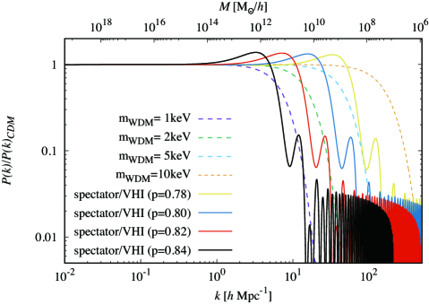
A modification of the initial power spectrum could act similar to warm dark matter at the dwarf galaxy scale in the present Universe. In Fig. 4, the ratio of the linear matter power spectra at between the spectator VHI model and the plain CDM model, is shown. In both models, the spectral index at the reference scale of is taken as and other cosmological parameters are assumed as and [57], where and are density parameters for baryon and CDM, is the Hubble parameter and is the amplitude of primordial power spectrum at the reference scale. For the spectator VHI model, we have chosen the model parameters, and , for a fixed value of in such a way that we obtain the above values of and at the reference scale. By fixing the model parameters in this way, the number of -folds corresponding to the mode are and for and , respectively. For guidance, as dashed lines, we also include several WDM models, assuming thermal relics of masses in the range keV. It can be seen that, compared to WDM models, the power spectrum in the spectator model begins to deviate at significantly larger scales.
Depending on the model parameters, the reduction of the primordial power, and the modification of the transfer function, discussed in Section 3, can result in either a reduction or boost of the linear matter power spectrum on galactic and supergalactic scales. Below the cut-off scale , there is a sharp suppression, more rapid than in the WDM case. Defining the “filtering mass” as the scale where the abundance of halos is suppressed by half relative to the standard model [15], we see that the spectator-VHI model with has a similar filtering scale to a WDM model with keV, near the lower limits allowed by Lyman- observations [11].
The scale-dependence of the WDM or VHI models relative to the standard model, however, is quite different: We see that the WDM models change the power by less than only half an order of magnitude above the filtering scale, while in the spectator model, there is an even weaker suppression on large scales, followed by a boost of on intermediate scales. Models based on observed stellar kinematics, abundance matching, and direct hydrodynamic cosmological simulations, place the lowest-mass dwarf galaxies in dark matter halos around . While WDM solutions to the postulated plain CDM failures in this regime would affect only a very narrow mass range, the signature of the spectator model would lead to a weak change in galaxy abundance over a range of masses and affect different scales in the Lyman- forest. At the very low mass end, just below the filtering scale, the spectator model predicts a very sharp decline in power. For a filtering mass of (corresponding to the peak mass of typical Milky Way dwarf spheroidals), the abundance of substructures below is greatly reduced in the WDM model, but for the spectator model, such substructures are non-existent. In this regime, where structures can only be detected indirectly, even a very small number of detections could therefore place significant constraints on spectator models.
In combination, this makes the spectator model clearly falsifiable. Quantitative predictions will require full, cosmological and hydrodynamic simulations, and will be the subject of future work.
5 Conclusion and Discussion
We have argued that, in models with a spectator field in the framework of a small-field inflation, after the inflaton-driven expansion there generically arises a second inflationary epoch which is driven by the spectator field. Depending on model parameters, the second inflation can generate the large number of -folds, possibly even . In this case, CMB scale fluctuations correspond to the modes which exited the horizon at when counted from the end of the first inflation. Let us recall that this is a very small number compared to the standard scenario where . Galactic scales correspond to the perturbations exiting around the very end of the first inflation.
As we discussed in Section 2, in the case of small-field inflation, the spectator fluctuations tend to give a negligible contribution. As a result, primordial power spectrum on small scales can be much suppressed compared to the standard plain CDM model while on large scales, the prediction can be consistent with observations of CMB. This is demonstrated in Fig. 4. Hence a model of the type with two periods of inflation would give interesting implications for the tension between small and large scale structure such as is manifest in “missing satellites” and “too big to fail” problems. As baryonic physics strongly regulate galaxy formation on these scales, a quantitative investigation of this issue will require cosmological hydrodynamic simulations, which are left for future work.
Recent weak lensing results from KiDS [58] continue to yield smaller than the value implied by the Planck data by to . There are extensions of the plain CDM model devised to alleviate the apparent tension; these include allowing for the curvature of the Universe, adopting dark energy models with a time-varying equation of state, modifying general relativity, assuming decaying dark matter (see e.g., [58] for a recent discussion).
While the linear matter power spectrum shown in Fig. 4 also suggests a large-scale effect of the modified transfer function, at low redshifts, this is likely to be washed out due to mode coupling in the full, non-linear evolution. More promising are observations of the 21cm forest around the time of reionisation, which could be able to either detect or rule out the characteristic bump in the power spectrum resulting from our model. With SKA promising to make these measurements during the next decade [14], more detailed numerical studies of the non-linear evolution in different inflation models seem to be particularly timely.
Acknowledgments
The authors also thank Baojiu Li, Matteo Leo, Mark Lovell and Kasper Siilin for helpful comments and suggestions. T.T. would like to thank the Helsinki Institute of Physics for the hospitality during the visit, where this work was done. T.S. is an Academy of Finland Research Fellow and supported by grant number 314238. T.T is supported by JSPS KAKENHI Grant Number 15K05084, 17H01131 and MEXT KAKENHI Grant Number 15H05888.
References
- [1] A. A. Klypin, A. V. Kravtsov, O. Valenzuela and F. Prada, Astrophys. J. 522 (1999) 82 [astro-ph/9901240].
- [2] B. Moore, S. Ghigna, F. Governato, G. Lake, T. R. Quinn, J. Stadel and P. Tozzi, Astrophys. J. 524 (1999) L19 [astro-ph/9907411].
- [3] Larson, R. B., Mon. Not. R. Astron. Soc. 169 (1974) 229.
- [4] Efstathiou, G., Mon. Not. R. Astron. Soc. 256 (1992) 43.
- [5] M. Boylan-Kolchin, J. S. Bullock and M. Kaplinghat, Mon. Not. Roy. Astron. Soc. 415 (2011) L40 [arXiv:1103.0007 [astro-ph.CO]].
- [6] T. Sawala et al., Mon. Not. Roy. Astron. Soc. 457 (2016) no.2, 1931 [arXiv:1511.01098 [astro-ph.GA]].
- [7] R. E. Gonzalez, A. V. Kravtsov and N. Y. Gnedin, Astrophys. J. 793 (2014) 91 [arXiv:1312.2587 [astro-ph.CO]].
- [8] M. R. Lovell et al., Mon. Not. Roy. Astron. Soc. 468 (2017) no.4, 4285 [arXiv:1611.00010 [astro-ph.GA]].
- [9] B. Bozek et al., Mon. Not. Roy. Astron. Soc. 483 (2019) no.3, 4086 [arXiv:1803.05424 [astro-ph.GA]].
- [10] J. A. Schewtschenko, C. M. Baugh, R. J. Wilkinson, C. Bœhm, S. Pascoli and T. Sawala, Mon. Not. Roy. Astron. Soc. 461 (2016) no.3, 2282 [arXiv:1512.06774 [astro-ph.CO]].
- [11] M. Viel, G. D. Becker, J. S. Bolton and M. G. Haehnelt, Phys. Rev. D 88 (2013) 043502 [arXiv:1306.2314 [astro-ph.CO]].
- [12] V. Iršič et al., Phys. Rev. D 96 (2017) no.2, 023522 [arXiv:1702.01764 [astro-ph.CO]].
- [13] R. Kennedy, C. Frenk, S. Cole and A. Benson, Mon. Not. Roy. Astron. Soc. 442 (2014) no.3, 2487 [arXiv:1310.7739 [astro-ph.CO]].
- [14] L. V. E. Koopmans et al., PoS AASKA 14 (2015) 001 doi:10.22323/1.215.0001 [arXiv:1505.07568 [astro-ph.CO]].
- [15] P. Bode, J. P. Ostriker and N. Turok, Astrophys. J. 556 (2001) 93 [astro-ph/0010389].
- [16] M. Kamionkowski and A. R. Liddle, Phys. Rev. Lett. 84, 4525 (2000) [astro-ph/9911103].
- [17] J. Yokoyama, Phys. Rev. D 62, 123509 (2000) [astro-ph/0009127].
- [18] T. Nakama, J. Chluba and M. Kamionkowski, Phys. Rev. D 95, no. 12, 121302 (2017) [arXiv:1703.10559 [astro-ph.CO]].
- [19] K. Enqvist, T. Meriniemi and S. Nurmi, JCAP 1407, 025 (2014) [arXiv:1404.3699 [hep-ph]].
- [20] K. Enqvist, S. Nurmi and S. Rusak, JCAP 1410, no. 10, 064 (2014) [arXiv:1404.3631 [astro-ph.CO]].
- [21] K. Enqvist, S. Nurmi, S. Rusak and D. Weir, JCAP 1602, no. 02, 057 (2016) [arXiv:1506.06895 [astro-ph.CO]].
- [22] K. Enqvist and M. S. Sloth, Nucl. Phys. B 626, 395 (2002) [arXiv:hep-ph/0109214].
- [23] D. H. Lyth and D. Wands, Phys. Lett. B 524, 5 (2002) [arXiv:hep-ph/0110002].
- [24] T. Moroi and T. Takahashi, Phys. Lett. B 522, 215 (2001) [Erratum-ibid. B 539, 303 (2002)] [arXiv:hep-ph/0110096].
- [25] G. Dvali, A. Gruzinov, M. Zaldarriaga, Phys. Rev. D69, 023505 (2004). [astro-ph/0303591].
- [26] L. Kofman, [astro-ph/0303614].
- [27] A. A. Starobinsky, Lect. Notes Phys. 246, 107 (1986).
- [28] K. Enqvist, R. N. Lerner, O. Taanila and A. Tranberg, JCAP 1210, 052 (2012) [arXiv:1205.5446 [astro-ph.CO]].
- [29] R. J. Hardwick, V. Vennin, C. T. Byrnes, J. Torrado and D. Wands, JCAP 1710, 018 (2017) [arXiv:1701.06473 [astro-ph.CO]].
- [30] D. Langlois and F. Vernizzi, Phys. Rev. D 70, 063522 (2004) [arXiv:astro-ph/0403258].
- [31] T. Moroi, T. Takahashi and Y. Toyoda, Phys. Rev. D 72, 023502 (2005) [arXiv:hep-ph/0501007].
- [32] K. Ichikawa, T. Suyama, T. Takahashi and M. Yamaguchi, Phys. Rev. D 78, 023513 (2008) [arXiv:0802.4138 [astro-ph]].
- [33] K. Dimopoulos, K. Kohri, D. H. Lyth and T. Matsuda, JCAP 1203, 022 (2012) [arXiv:1110.2951 [astro-ph.CO]].
- [34] G. Lazarides, R. R. de Austri and R. Trotta, Phys. Rev. D 70, 123527 (2004) [hep-ph/0409335].
- [35] T. Moroi and T. Takahashi, Phys. Rev. D 72, 023505 (2005) [arXiv:astro-ph/0505339];
- [36] J. Fonseca and D. Wands, JCAP 1206, 028 (2012) [arXiv:1204.3443 [astro-ph.CO]].
- [37] K. Enqvist and T. Takahashi, JCAP 1310 (2013) 034 [arXiv:1306.5958 [astro-ph.CO]].
- [38] V. Vennin, K. Koyama and D. Wands, JCAP 1511, 008 (2015) [arXiv:1507.07575 [astro-ph.CO]].
- [39] T. Fujita, M. Kawasaki and S. Yokoyama, JCAP 1409, 015 (2014) [arXiv:1404.0951 [astro-ph.CO]].
- [40] N. Haba, T. Takahashi and T. Yamada, JCAP 1806, no. 06, 011 (2018) [arXiv:1712.03684 [hep-ph]].
- [41] K. Ichikawa, T. Suyama, T. Takahashi and M. Yamaguchi, Phys. Rev. D 78, 063545 (2008) [arXiv:0807.3988 [astro-ph]].
- [42] A. A. Starobinsky, JETP Lett. 42 (1985) 152 [Pisma Zh. Eksp. Teor. Fiz. 42 (1985) 124].
- [43] M. Sasaki and E. D. Stewart, Prog. Theor. Phys. 95, 71 (1996) [arXiv:astro-ph/9507001].
- [44] M. Sasaki and T. Tanaka, Prog. Theor. Phys. 99, 763 (1998) [arXiv:gr-qc/9801017].
- [45] J. Martin, C. Ringeval and V. Vennin, Phys. Dark Univ. 5-6, 75 (2014) [arXiv:1303.3787 [astro-ph.CO]].
- [46] S. E. Hong, H. J. Lee, Y. J. Lee, E. D. Stewart and H. Zoe, JCAP 1506, 002 (2015) [arXiv:1503.08938 [astro-ph.CO]].
- [47] M. Leo, C. M. Baugh, B. Li and S. Pascoli, JCAP 1812, no. 12, 010 (2018) [arXiv:1807.04980 [astro-ph.CO]].
- [48] A. Lewis, A. Challinor and A. Lasenby, Astrophys. J. 538, 473 (2000) [astro-ph/9911177].
- [49] C. Boehm, A. Riazuelo, S. H. Hansen and R. Schaeffer, Phys. Rev. D 66 (2002) 083505 [astro-ph/0112522].
- [50] M. Vogelsberger, J. Zavala and A. Loeb, Mon. Not. Roy. Astron. Soc. 423 (2012) 3740 [arXiv:1201.5892 [astro-ph.CO]].
- [51] M. Vogelsberger, J. Zavala, K. Schutz and T. R. Slatyer, arXiv:1805.03203 [astro-ph.GA].
- [52] X. D. Shi and G. M. Fuller, Phys. Rev. Lett. 82 (1999) 2832 [astro-ph/9810076].
- [53] T. Sawala, C. S. Frenk, R. A. Crain, A. Jenkins, J. Schaye, T. Theuns and J. Zavala, Mon. Not. Roy. Astron. Soc. 431 (2013) 1366 [arXiv:1206.6495 [astro-ph.CO]].
- [54] O. Newton, M. Cautun, A. Jenkins, C. S. Frenk and J. C. Helly, arXiv:1809.09625 [astro-ph.GA].
- [55] T. Sawala, P. Pihajoki, P. H. Johansson, C. S. Frenk, J. F. Navarro, K. A. Oman and S. D. M. White, Mon. Not. Roy. Astron. Soc. 467 (2017) no.4, 4383 [arXiv:1609.01718 [astro-ph.GA]].
- [56] S. Bose et al., Mon. Not. Roy. Astron. Soc. 464, no. 4, 4520 (2017) [arXiv:1604.07409 [astro-ph.CO]].
- [57] P. A. R. Ade et al. [Planck Collaboration], Astron. Astrophys. 594, A13 (2016) [arXiv:1502.01589 [astro-ph.CO]].
- [58] S. Joudaki et al., Mon. Not. Roy. Astron. Soc. 474, no. 4, 4894 (2018) doi:10.1093/mnras/stx2820 [arXiv:1707.06627 [astro-ph.CO]].