A Distributed Optimization Algorithm over Time-Varying Graphs with Efficient Gradient Evaluations
Abstract
We propose an algorithm for distributed optimization over time-varying communication networks. Our algorithm uses an optimized ratio between the number of rounds of communication and gradient evaluations to achieve fast convergence. The iterates converge to the global optimizer at the same rate as centralized gradient descent when measured in terms of the number of gradient evaluations while using the minimum number of communications to do so. Furthermore, the iterates converge at a near-optimal rate when measured in terms of the number of communication rounds. We compare our algorithm with several other known algorithms on a distributed target localization problem.
1 Introduction
We consider the distributed optimization problem
| (1) |
Associated with each agent is the local objective function where is the number of agents and is the dimension of the problem. The goal is for all the agents to calculate the global optimizer using only local communications and gradient evaluations.
Many algorithms have been proposed recently to solve the distributed optimization problem. Some examples include distributed gradient descent by Nedić and Ozdaglar (2009), EXTRA by Shi et al. (2015), AugDGM by Xu et al. (2015), NIDS by Li et al. (2017), DIGing by Nedić et al. (2017) and Qu and Li (2018), Exact Diffusion by Yuan et al. (2019), and SVL by Sundararajan et al. (2019) among others. In each algorithm, agents do the following at each step:
-
•
communicate state variables with local neighbors,
-
•
evaluate the local gradient , and
-
•
update local state variables.
Each algorithm alternates between these three steps and therefore uses the same number of communications and local gradient evaluations. In this paper, however, we allow this ratio to depend on the properties of the objective function and the communication network. To characterize the convergence properties of our algorithm, we use the following notions of time.
-
•
We define a step as one round of communication and at most one gradient evaluation.
-
•
We define an iteration as rounds of communication and one gradient evaluation.
In other words, an iteration consists of steps where each step is at least as simple as that of the algorithms previously mentioned. We assume that local state updates have neglible cost and can therefore be performed any number of times per step or iteration.
For example, consider an algorithm that updates as follows:
| iteration | 1 | 2 | 3 | ||||||
|---|---|---|---|---|---|---|---|---|---|
| step | 1 | 2 | 3 | 4 | 5 | 6 | 7 | 8 | 9 |
| communication | ✓ | ✓ | ✓ | ✓ | ✓ | ✓ | ✓ | ✓ | ✓ |
| gradient evaluation | ✓ | ✓ | ✓ |
-
(1)
The iterates of our algorithm converge to the optimizer with the same rate as centralized gradient descent in terms of number of the iterations. Furthermore, our algorithm achieves this using the minimum number of communications per gradient evaluation.
-
(2)
The iterates of our algorithm converge to the optimizer with a near-optimal rate in terms of the number of steps, despite not evaluating the gradient at each step.
-
•
The local objective functions satisfy a contraction property that is weaker than assuming smoothness and strong convexity.
-
•
The communication network may be time-varying and either directed or undirected as long as it is sufficiently connected and the associated weight matrix is doubly stochastic at each step.
2 Problem setup
We now discuss the assumptions on the objective function and the communication network that we make in order to solve the distributed optimization problem (1).
2.1 Objective function
Assumption 1
The distributed optimization problem (1) has an optimizer . Furthermore, there exists a stepsize and contraction factor such that
| (2) |
for all and all .
Each is in general nonzero, although we have
| (3) |
Assumption 1 also implies that
so the global objective function satisfies the same property as the local functions. Assumption 1 holds if the local functions satisfy a one-point smooth and strong convexity property as described in the following proposition.
Proposition 1
Let , and suppose each local function is one-point -smooth and -strongly convex with respect to the global optimizer, in other words,
for all and all . Then (2) holds with stepsize and contraction factor .
Assumption 1 also holds under the stronger assumption that each is -smooth and -strongly convex, meaning that
for all and all .
2.2 Communication network
To characterize the communication among agents, we use a gossip matrix defined as follows.
Definition 2 (Gossip matrix)
We say that the matrix is a gossip matrix if whenever agent does not receive information from agent . We define the spectral gap of a gossip matrix as
| (4) |
Furthermore, we say that is doubly-stochastic if both and .
The spectral gap characterizes the connectivity of the communication network. In particular, a small spectral gap corresponds to a well-connected network and vice versa. One way to obtain a gossip matrix is to set where is the (possibly weighted) graph Laplacian. We make the following assumption about the gossip matrix.
Assumption 2 (Communication network)
There exists a scalar such that each agent has access to the row of a doubly-stochastic gossip matrix with spectral gap at most at each step of the algorithm.
Time-varying communication networks that are either directed or undirected can satisfy Assumption 2 as long as the associated gossip matrix is doubly stochastic with a known upper bound on its spectral gap. See Xiao et al. (2007) for how to optimize the weights of the gossip matrix to minimize the spectral gap, and see Nedić and Olshevsky (2015) for distributed optimization over non-doubly-stochastic networks using the push-sum protocol.
2.3 Centralized gradient descent
The (centralized) gradient descent iterations are given by
| (5) |
where is the stepsize. Under Assumption 1, this method converges to the optimizer linearly with rate . In other words, . While this method could be approximated in a decentralized manner using a large number of steps per iteration (so that every agent can compute the average gradient at each iteration), we show that our algorithm achieves the same convergence rate using the minimal number of necessary rounds of communication per gradient evaluation.
3 Main Results
To solve the distributed optimization problem, we now introduce our algorithm, which depends on the stepsize , contraction factor , and spectral gap .
-
•
Each agent chooses such that (for example, ).
-
•
Define the number of communications per iteration
At iteration of the algorithm, agent first communicates with its local neighbors times using the gossip matrices , then evaluates its local gradient at the point resulting from the communication, and finally updates its local state variables and . The output of the algorithm is , which is the estimate of the optimizer of the global objective function . Note that agents are required to know the global parameters and so that they can calculate the number of communication rounds .
For a given contraction factor and spectral gap , agents perform consecutive rounds of communication at each iteration where
| (6) |
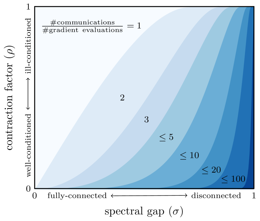
This is the minimum integer number of communication rounds so that the spectral gap of the -step gossip matrix at iteration is no greater than . Since only one gradient evaluation is performed per iteration, this adjusts the ratio between the number of communications and gradient evaluations as shown in Figure 1. In particular, the algorithm uses a single communication per gradient evaluation when the network is sufficiently connected ( small) and the objective function is ill-conditioned ( large). As the network becomes more disconnected and/or the objective function becomes more well-conditioned, the algorithm uses more communications per gradient evaluation in order to keep the ratio at the optimal operating point.
We now present our main result, which states that the iterates of each agent converge to the global optimizer linearly with a rate equal to the contraction factor . We prove the result in Appendix A.
Theorem 3.0 (Main result)
Theorem 1 states that the iterates of our algorithm converge to the optimal solution of (1) in a decentralized manner at the same rate as centralized gradient descent (5) in terms of the number of iterations. In other words, the algorithm converges just as fast (in the worst case) as if each agent had access to the information of all other agents at every iteration. Instead of communicating all this information, however, it is sufficient to only perform rounds of communication where is defined in (6).
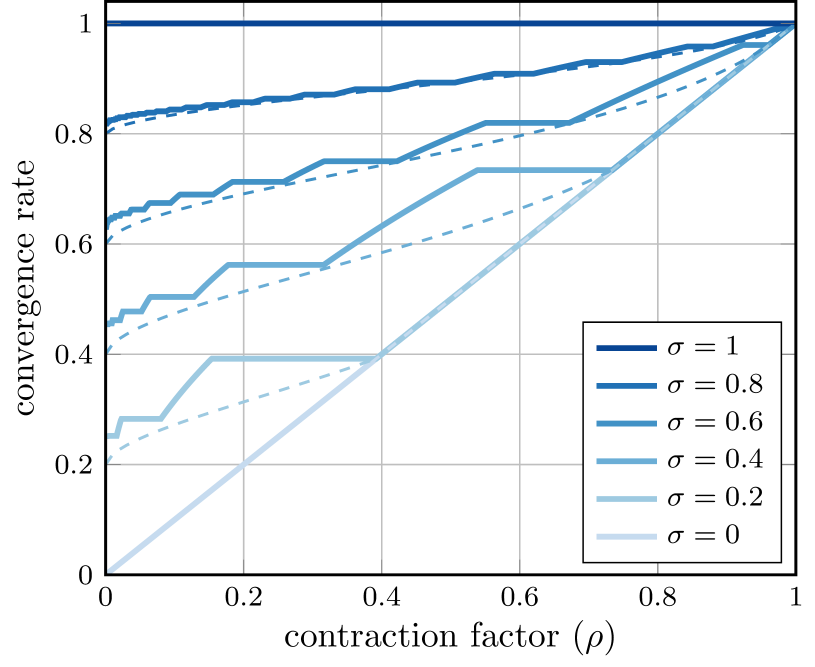
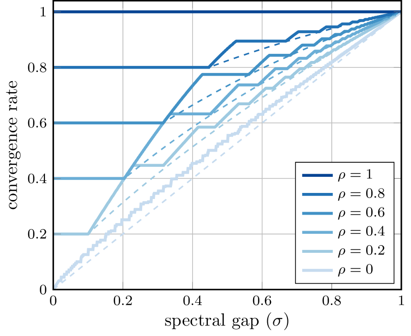
The convergence rate in Theorem 1 is in terms of the number of iterations. To compare the performance of our algorithm in terms of the number of steps, we plot the convergence rate per step in Figure 2. For comparison, we also plot the rate of the algorithm SVL by Sundararajan et al. (2019). This algorithm is designed to optimize the convergence rate per step and requires agents to compute their local gradient at each step of the algorithm. In contrast, our algorithm is slightly slower than the optimal algorithm but uses far fewer computations since local gradients are only evaluated once every steps.
4 Application: Target Localization
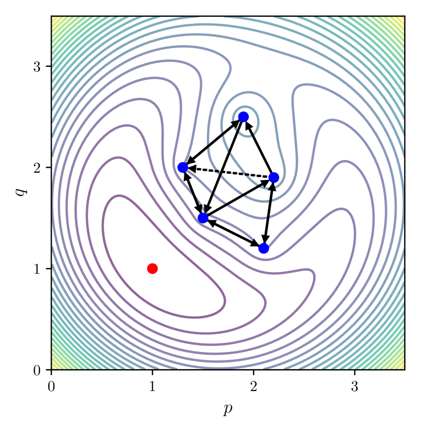
To illustrate our results, we use our algorithm to solve the distributed target localization problem illustrated in Figure 3, which is inspired by the example in Section 18.3 of the book by Boyd and Vandenberghe (2018). We assume each agent (blue dot) can measure its distance (but not angle) to the target (red dot) and can communicate with local neighbors.
Suppose agents are located in a two-dimensional plane where the location of agent is given by . Each agent knows its own position but not the location of the target, denoted by . Agent is capable of measuring its distance to the target,
The objective function associated to agent is
Then in order to locate the target, the agents cooperate to solve the distributed nonlinear least-squares problem
| (8) |
Agents can communicate with local neighbors as shown in Figure 3. To simulate randomly dropped packets from agent to agent , the gossip matrix at each iteration is randomly chosen from the set
Both gossip matrices satisfy Assumption 2 with maximum spectral gap .
We choose the stepsize to optimize the asymptotic rate of convergence. In particular, the estimate of each agent becomes arbitrarily close to the target as , so the optimal stepsize is where and are the smallest and largest eigenvalues of the Hessian matrix evaluated at the target, in other words, . Since the objective function is two-dimensional, the sum of its smallest and largest eigenvalues is equal to its trace, so
where the trace of the local Hessian is
The trace is equal to one at the target, so the optimal stepsize is . Since NIDS and EXTRA are unstable with this stepsize, we instead use and , respectively, for these algorithms. The parameters of SVL are completely determined by and .
We choose the contraction factor as the convergence rate of centralized gradient descent which is . Then our algorithm performs communication rounds per iteration. We have each agent initialize its states with its position and .
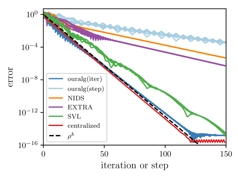
In Figure 4, we plot the error of each agent as a function of either the iteration or step. As expected from Theorem 1, the error of our algorithm converges to zero at the same rate as centralized gradient descent (5) in terms of iterations. Our algorithm uses communications per iteration while NIDS, EXTRA, and SVL use only one; our algorithm is more efficient in terms of gradient evaluations, but also uses more communications than the other algorithms to obtain a solution with a given precision.
5 Conclusion
We developed an algorithm for distributed optimization that uses the minimal amount of communication necessary such that the iterates converge to the optimizer at the same rate as centralized gradient descent in terms of the number of gradient evaluations. Furthermore, the convergence rate of our algorithm is near-optimal (in the worst-case) in terms of the number of communication rounds even though the gradient is not evaluated at each step. Such an algorithm is particularly useful when gradient evaluations are expensive relative to the cost of communication.
References
- Boyd and Vandenberghe (2018) Boyd, S. and Vandenberghe, L. (2018). Introduction to Applied Linear Algebra – Vectors, Matrices, and Least Squares. Cambridge University Press, New York, NY, USA.
- Li et al. (2017) Li, Z., Shi, W., and Yan, M. (2017). A decentralized proximal-gradient method with network independent step-sizes and separated convergence rates. arXiv:1704.07807.
- Nedić and Olshevsky (2015) Nedić, A. and Olshevsky, A. (2015). Distributed optimization over time-varying directed graphs. IEEE Transactions on Automatic Control, 60(3), 601–615.
- Nedić et al. (2017) Nedić, A., Olshevsky, A., and Shi, W. (2017). Achieving geometric convergence for distributed optimization over time-varying graphs. SIAM Journal on Optimization, 27(4), 2597–2633.
- Nedić and Ozdaglar (2009) Nedić, A. and Ozdaglar, A. (2009). Distributed subgradient methods for multi-agent optimization. IEEE Transactions on Automatic Control, 54(1), 48–61.
- Qu and Li (2018) Qu, G. and Li, N. (2018). Harnessing smoothness to accelerate distributed optimization. IEEE Transactions on Control of Network Systems, 5(3), 1245–1260.
- Scaman et al. (2017) Scaman, K., Bach, F., Bubeck, S., Lee, Y.T., and Massoulié, L. (2017). Optimal algorithms for smooth and strongly convex distributed optimization in networks. In Proceedings of the 34th International Conference on Machine Learning, volume 70 of Proceedings of Machine Learning Research, 3027–3036.
- Shi et al. (2015) Shi, W., Ling, Q., Wu, G., and Yin, W. (2015). EXTRA: An exact first-order algorithm for decentralized consensus optimization. SIAM Journal on Optimization, 25(2), 944–966.
- Sundararajan et al. (2019) Sundararajan, A., Van Scoy, B., and Lessard, L. (2019). Analysis and design of first-order distributed optimization algorithms over time-varying graphs. arXiv:1907.05448.
- Xiao et al. (2007) Xiao, L., Boyd, S., and Kim, S.J. (2007). Distributed average consensus with least-mean-square deviation. Journal of Parallel and Distributed Computing, 67(1), 33–46.
- Xu et al. (2015) Xu, J., Zhu, S., Soh, Y.C., and Xie, L. (2015). Augmented distributed gradient methods for multi-agent optimization under uncoordinated constant stepsizes. In IEEE Conference on Decision and Control, 2055–2060.
- Yuan et al. (2019) Yuan, K., Ying, B., Zhao, X., and Sayed, A.H. (2019). Exact diffusion for distributed optimization and learning—Part I: Algorithm development. IEEE Transactions on Signal Processing, 67(3), 708–723.
Appendix A Proof of Theorem 1
We now prove linear convergence of the iterates of our algorithm to the optimizer of the global objective function.
Average and disagreement operators. To simplify the notation, we define the average operator as
along with the disagreement operator as
where denotes the Kronecker product. Note that any point can be decomposed into its average and disagreement components since . Also, the operators are orthogonal in that for all .
Vectorized form. Defining the parameter , we can then write our algorithm in vectorized form as
| (9a) | ||||
| (9b) | ||||
| (9c) | ||||
| (9d) | ||||
with where the concatenated vectors are
and the -step consensus operator and global gradient operator are defined as111We use the over-bar in to distinguish it from the gradient of the global objective function in (1). The operators are related by .
Fixed-point. Define the points as
Then is a fixed-point of the concatenated system (9) since the gossip matrix is doubly-stochastic at each step. Also, since satisfies (3).
Error system. To analyze the algorithm, we use a change of variables to put it in error coordinates. The error vectors
satisfy the iterations
| (10a) | ||||
| (10b) | ||||
for .
Fixed-point operator. From Assumption 1, the global gradient operator satisfies
and
| (11) |
for all . In other words, is a contraction with respect to the point with contraction factor .
Consensus operator. From Assumption 2 along with the definition of , the consensus operator satisfies
| (12) |
for all and all where
Consensus direction. We now derive some properties of the average error vectors. Using the assumption that the gossip matrix is doubly-stochastic, we have
| (13) |
The iterates are initialized such that (recall that ). Taking the average of (9c), we have that the average is preserved. In other words, we have that for all . Then by induction,
| (14) |
Lyapunov function. To prove convergence, we will show that the function defined by
| (15) |
is a Lyapunov function for the algorithm, that is, it is both positive definite and decreasing along system trajectories. Note that since , so the matrix in (15) is positive definite. Then is also positive definite, meaning that for all and , and if and only if and (recall that ). Next, we show that the Lyapunov function decreases by a factor of at least at each iteration. Define the weighted difference in the Lyapunov function between iterations as
Subsituting the expressions for the iterates in (10) and using the properties of the average iterates in (13) and (14), we have
The first term is nonpositive since satisfies (11), the second since satisfies (12), and the third since it is a squared norm. Therefore, for all . Applying this inequality at each iteration and summing, we obtain the bound
Bound. Finally, we use the Lyapunov function to show that converges to zero linearly with rate for each agent . The norm is upper bounded by
where the nonnegative constant is defined as
and denotes the condition number. Taking the square root, we obtain the bound
for each agent and iteration .