Towards Practical Indoor Positioning Based on Massive MIMO Systems

Abstract

We showcase the practicability of an indoor positioning system (IPS) solely based on Neural Networks and the channel state information (CSI) of a (Massive) multiple-input multiple-output (MIMO) communication system, i.e., only build on the basis of data that is already existent in today’s systems. As such our IPS system promises both, a good accuracy without the need of any additional protocol/signaling overhead for the user localization task. In particular, we propose a tailored NN structure with an additional phase branch as feature extractor and (compared to previous results) a significantly reduced amount of trainable parameters, leading to a minimization of the amount of required training data. We provide actual measurements for indoor scenarios with up to 64 antennas covering a large area of $80\text{\,}\mathrm{m}^{2}$. In the second part, several robustness investigations for real-measurements are conducted, i.e., once trained, we analyze the recall accuracy over a time-period of several days. Further, we analyze the impact of pedestrians walking in-between the measurements and show that finetuning and pre-training of the NN helps to mitigate effects of hardware drifts and alterations in the propagation environment over time. This reduces the amount of required training samples at equal precision and, thereby, decreases the effort of the costly training data acquisition.

I Introduction

Mobile communication devices such as smartwatches and smartphones have become companions of everyday’s life, resulting in a rich variety of new possible use-cases and applications in almost any area of modern life. While constant connectivity and endless computational resources have become omnipresent, the seemingly simple problem of estimating one’s position inside buildings has not yet been finally resolved [1]. Therefore, a need for IPSs is created, as IPSs can be seen as a key enabler for a wide range of applications such as indoor navigation, smart factories, or could even provide a basic security functionality in distributed internet of things (IoT) sensor networks. Contrary to the outdoor scenario where global positioning system (GPS) provides a single universal solution for almost any possible location (assuming Line-of-Sight (LoS) to the satellite), IPSs are characterized by a heterogeneous problem formulation and, thus, also many different solutions have been proposed in the literature. Moreover, also for the outdoor scenario, such a positioning system can be of practical interest as it may enhance precoding of Massive MIMO systems through predicting the users’ movements directly in the base station (BS). While the LoS scenario is well-understood and multiple technologies are reported in the literature [2, 3, 4] (e.g., angle- and time-of-arrival based predictions and triangulation methods) suitable solutions for more general channels (e.g., the much more complex Non-Line-of-Sight (NLoS) scenario) with all its practical impairments are still open for research. Note that in the following we only focus on radio frequency (RF)-based technologies as it can be embedded into current systems without the need of additional sensors.

Obviously, there exists a trade-off between achievable accuracy and required overhead in terms of spectrum and computational complexity. In this work, we focus on rather inaccurate (targeting sub-m precision) but low-overhead systems based on CSI that can be implemented on top of existing communication standards. This seems to be sufficient for many applications such as indoor navigation in public buildings or movement prediction of the user equipment (UE) within a BS. Thus, different approaches have been proposed (compare to [5, 6, 7]) and investigated in the past, each optimized for different applications and system models. Overall, these approaches can be split into two categories, where obviously mixtures between both categories exist:

1. Model-based: define how the channel is expected to behave and estimate the position accordingly (e.g. ray-tracing)

2. Data-driven: collect a database with appropriate features (often called fingerprints) and corresponding positions (e.g., CSI [8, 9], received signal strength indicator (RSSI) [10, 11] and recently time-reversal IPS (TRIPS) [12]), i.e., somehow interpolate in-between.

It was proposed to combine IPS with Massive MIMO [13, 14, 15, 16, 17], as it uses an over-provisioning of antennas to separate users in space and thereby creates an $N_{\text{Ant}}$ antenna times $N_{\text{sub}}$ subcarrier fingerprint per spatial position as a side product. Thus, Massive MIMO appears to be an attractive candidate for enabling robust IPSs.

Although there exists an underlying channel transfer function which describes the behavior of the channel for any given position, this function is typically not known or can only be approximated, as it is infeasible to fully capture the geometries of the environment and its surrounding area. This results in the emerging of classical machine learning techniques [18] to exploit the typical channel behavior for predicting a user’s spatial position. Moreover, it was proposed in [19, 15, 16] to neglect any pre-processing which extracts channel features based on expert-knowledge, and rather directly work with raw CSI. The intuition behind is that an NN should be able to approximate such functions, without the need of any a priori knowledge other than the observed measured data. This ease in modeling and flexibility in application comes at the cost of acquiring a (typically) larger quantity of channel estimates.

It was shown in [16] that the data-driven approach can, in principle, achieve sub-cm precision, but entails an overhead of sampling large datasets per environment, and it is unclear how many samples are required to achieve a target precision. Therefore, we investigate the influence of the amount of data samples on the prediction accuracy for standard LoS and NLoS indoor channels. To improve these state-of-the-art systems, tracking over recurrent neural network (RNN) was proposed in [20, 21], resulting in a more robust system. Although Massive MIMO in combination with IPS was extensively studied in [13, 14, 15, 16, 17], the influence of the number of antennas and different practical implementation challenges (e.g., hardware impairments and time varying drifts) influencing the precision and robustness of the system have yet to be studied in detail.

In addition, measurements tend to be captured over a short period of time and, thereby, often there is a lack of verifiable reproducibility of results over a longer period of time. Thus, we also investigated time dynamic effects by conducting a measurement campaign over several week days. For this, we train an NN based on data captured at a specific day of the week, e.g. Monday, and then predicted positions based on data from another day, showing a slight performance degradation. To counter this degradation, we show that finetuning and pre-training help to mitigate those time drifting effects and also to reduce the amount of data points needed for training. Finally, we also address another major practical burden, namely the fact that most of the time a static environment is investigated without considering any time-dependent disturbances in-between BS and UE, e.g., caused by pedestrians walking around as obstacles.

II Background

It is widely accepted that Massive MIMO unleashes its full potential only in combination with time division duplexing (TDD) as the piloting overhead is independent of the number of BS antennas $N_{\text{Ant}}$ [22]. For simplicity, we assume that a UE is only equipped with a single antenna, but extensions are straightforward. Further, we use orthogonal frequency division multiplex (OFDM), i.e., $N_{\text{sub}}$ subcarriers exist.

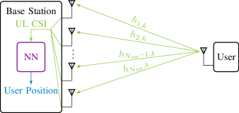
For standard communication in TDD Massive MIMO the UEs transmit orthogonal pilots to the BS and the BS uses these pilots to estimate the channel at antenna $m$ $\hat{\mathbf{h}}_{m,k}\in\mathbb{C}^{N_{\text{Ant}}\times N_{\text{sub}}}$ per subcarrier $k$ as shown in Fig. 1. This estimate of the channel (CSI) is then used to orthogonalize the users in space. In the following, we reuse this CSI to create a robust fingerprint for each spatial position $x,y,z$ of the UE.

Figure 1: System schematic for predicting a user’s position with an NN based on UL CSI.

To compare the prediction performance we use two different metrics:

1. The mean distance error (MDE)

   $$\acs{MDE}=\frac{1}{N_{\text{test}}}\sum^{N_{\text{test}}}_{n=1}\|\mathbf{d}_{n}-\hat{\mathbf{d}_{n}}\|_{2}$$ (1)

   is used for simulated data, where the average distance error (DE) is calculated over the whole test size $N_{\text{test}}$.

2. Since this metric punishes outliers, we use the mean distance accuracy (MDA) for measured data (compare [19]). MDA is defined as the DE that 50% of the users are achieving at least, which thereby removes the influence of heavy outliers that often occur in measurements.

II-A Simulated Channels

Figure 2: Simulation setup for the 3GPP channel model.

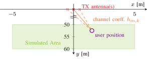
To show the viability of the proposed NN, we begin with an investigation on simulated standardized channel models for LoS and NLoS indoor scenarios. For this, we use the Quadriga Framework [23]. Fig. 2 illustrates the simulation setup, where a BS with the antenna geometry of an $8\times 8$ patch array is placed in the origin of the coordinates and an area of $100\text{\,}\mathrm{m}^{2}$ is simulated. The sampling resolution is $10\text{\,}\mathrm{cm}$ $<\lambda/2$ in both $x$ and $y$ direction. Further, an OFDM channel estimation with 1024 subcarriers and a bandwidth of $20\text{\,}\mathrm{MHz}$ around the carrier frequency of $1.25\text{\,}\mathrm{GHz}$ is used. These parameters are chosen to equal those of the actual measurement campaigns as presented in the later sections.

II-B Measured Channels

We provide a short introduction to the actual measurements that were conducted at our institute, as can be seen in Fig. 3. For the exact measurement procedure which inherently provides ground truth (i.e., 3D position labels) at centimeter precision, we refer the interested reader to [24].

Figure 3: Indoor measurement positions.

The transmitter (UE) consists of an amplified universal software radio peripheral (USRP) with a dipole antenna which transmits OFDM pilot symbols with 1024 subcarriers and a bandwidth of $20\text{\,}\mathrm{MHz}$ at $1.25\text{\,}\mathrm{GHz}$. For subcarrier modulation, a simple binary phase shift keying (BPSK) constellation was chosen. Note that 10% of the subcarriers are used as guard band and the cyclic prefix was 1/8 of the OFDM symbol duration. To be able to reuse the same NN structure for simulated and measured samples, the missing guard band subcarriers in measured samples were replaced by zeros to maintain the NN’s input size of $1024$ subcarriers.

TABLE I: Description of datasets.

Dataset	$\#$ Samples	Covered Area
Indoor Simulations	10000	$10\text{\,}\mathrm{m}$ $\times$ $10\text{\,}\mathrm{m}$=$100\text{\,}\mathrm{m}^{2}$
LoS Weekdays Measurements	6000	$40\text{\,}\mathrm{m}$ $\times$ $2\text{\,}\mathrm{m}$=$80\text{\,}\mathrm{m}^{2}$
Disturbed Indoor Measurement	5800	$40\text{\,}\mathrm{m}$ $\times$ $2\text{\,}\mathrm{m}$=$80\text{\,}\mathrm{m}^{2}$
NLoS Indoor Measurement	2700	$2\text{\,}\mathrm{m}$ $\times$ $18\text{\,}\mathrm{m}$=$36\text{\,}\mathrm{m}^{2}$

Tab. I gives an overview of the used datasets and their corresponding coverage areas, where the area dimensions match those in [19]. In the “LoS Weekdays Measurements” each day was measured with the same meander-like path structure, resulting in a sample distance of around $1\text{\,}\mathrm{cm}$. For the “Disturbed Indoor Measurement”, two colleagues were shadowing the antenna array by randomly walking in-between BS and UE.

III Proposed Neural Network Architecture

Figure 4: Basic structure of the proposed NN.

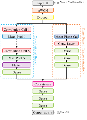
Fig. 4 depicts the layout of the proposed NN. As we treat complex values as two independent real numbers, the input of the NN has the shape

$$N_{\text{batch}}\times N_{\text{sub}}\times N_{\text{Ant}}\times 2.$$

where $N_{\text{sub}}$ is the number of subcarriers, $N_{\text{Ant}}$ is the number of antennas, and the fourth dimension is composed of the real and imaginary parts. A noise and a dropout layer is directly added to this input to prevent the NN from overfitting and to reinforce the NN not to rely on strong antennas only. Afterward, the graph is split in two branches, a “Convolutional Branch” and a “Phase Branch”. The “Convolutional Branch” is built of $5$ convolutional cells for evaluating the fingerprint in the amplitude of the real and imaginary part. Therefore, a 3-dimensional kernel of shape $X\times Y\times 2$ is used in the first convolutional layer, to combine real and imaginary parts, while subsequent layers use 2-dimensional kernels to further convolve over the subcarrier and antenna dimensions. The second branch, referred to as “Phase Branch”, further improves the MDE (simulated data)/ MDA (measured data), by focusing on the phase difference between antennas, which helps especially when measured data is used. Within this branch we explicitly calculate the mean phase per antenna over all subcarriers and then forward this refined information to the NN. Inserting such expert knowledge operations drastically reduces complexity that otherwise must be learned through exhaustive training. This is similar to the idea of transformer networks [25]. By doing so, the NN experiences a faster convergence and a higher final prediction accuracy. Finally, the two branches are concatenated and four fully connected dense layers are used to combine both outputs to arrive at a prediction of the user’s $x-,y-,z$-position.

During training, we use $N_{\text{train}}$ samples (i.e., data $\mathbf{v}$ and position labels $\mathbf{w}$) and apply multiple stochastic gradient descent iterations, where one iteration over the whole dataset is denoted asepochs $N_{\text{ep}}$. Thus, the same $N_{\text{train}}$ samples are considered $N_{\text{ep}}$ times, to find the best weights $\boldsymbol{\theta}$. We chose the Huber-loss [26] as loss metric during training and the absolute distance deviation to measure the accuracy. Intuitively, the optimal training signal-to-noise-ratio (SNR) is a trade-off between high noise power, i.e,. learning robustness to noisy data and noiseless samples, i.e., learning the underlying (deterministic) channel transfer function [27]. To further prevent overfitting, we used the previously mentioned dropout layer where we reached best performance and accuracy with a dropout rate of $10$\mathrm{\char 37\relax}$$. Additionally, the generalization effect of the dropout layer comes along with an improved prediction with respect to reproducibility in time for changing datasets, as will be shown later. We start the training procedure with mini-batch sizes of $16$ samples. After retraining for multiple epochs until an early stopping mechanism detects no further improvements, we then continue training with a stepwise increased batch size up to $512$ samples per batch. To achieve a higher final prediction accuracy, the learning rate is also reduced stepwise from $0.001$ to $0.00005$ before advancing to the next batch size.

TABLE II: Improvement by using a phase branch

Dataset	without	Phasebranch	Rel. Impr.
3GPP LoS	$0.1621\text{\,}\mathrm{m}$	$0.0863\text{\,}\mathrm{m}$	$46.1\text{\,}\mathrm{\char 37\relax}$
3GPP NLoS	$0.1275\text{\,}\mathrm{m}$	$0.1183\text{\,}\mathrm{m}$	$7.2\text{\,}\mathrm{\char 37\relax}$
Monday Mes.	$0.3467\text{\,}\mathrm{m}$	$0.2460\text{\,}\mathrm{m}$	$29.0\text{\,}\mathrm{\char 37\relax}$

Tab. II shows the gain of the proposed “Phase Branch” over traditional fingerprinting approaches, resulting in an improvement in measurements of $29\text{\,}\mathrm{\char 37\relax}$ by only adding $22000$ weights. It can be seen that for the simulated data and measured data the NN achieves (with a total of only 440.000 weights) the same accuracy as in [19] for a similar area and propagation environment (cf. Fig. in [19]).

III-A Required Training Data

In a practical use-case, training data is valuable as each sample has to be captured manually and also the ground truth position is required. Therefore, we investigate how the NN approach can deal with a larger grid resolution than the original one ($10\text{\,}\mathrm{cm}$) with 10.000 samples. To make a fair comparison we take every second/third/.. sample, in the mesh grid, i.e., create a larger sample distance. Note that the sample size is reduced quadratically (both dimensions $x$ and $y$).

Figure 5: Simulated: 3GPP LoS and NLoS outdoor MDE for different sample distances.

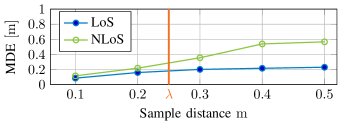
Fig.  5 shows the MDE for the different sample distances. In the LoS case the NN is able to resolve the positions even with a low grid resolution. The NLoS is far more dependent on a finer grid resolution, as it has less spatial correlation and inhibits more random components than the LoS case. Therefore the NN is less capable of interpolating in between the trained samples. From this it can be seen, that in the LoS case the NN learns a more robust representation of the LoS fingerprints than in the NLoS case.

III-B Influence of the Number of Antennas

In typical Massive MIMO scenarios the antenna gain and the ability to separate users increases with the number of antennas, therefore can be expected that by increasing the number of antennas the fingerprint and the overall system is more robust against different impairments. However, also the training complexity increases.

Figure 6: Simulated: MDE for the 3GPP LoS indoor channel models with different number of antennas, trained at a target $\acs{SNR}=$20\text{\,}\mathrm{dB}$$.

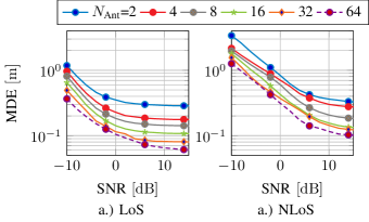
Fig. 6 illustrates the robustness of the proposed system for different number of antennas in the LoS case (left) and in the NLoS case (right). It can be seen that roughly a $3\text{\,}\mathrm{dB}$ gain per doubling the antenna occurs. But even with a low number of antennas the system still achieves reasonably good results in the case of LoS. For the NLoS case, more antennas are needed for achieving a robustness against measurement noise (curves are shifted to the right) and more antennas are needed to achieve similar accuracy as in the LoS case. This shows that the number of antennas enhances the robustness in all cases for IPS and that Massive MIMO is a good match for this system.

Figure 7: Measured: MDA with different numbers of antennas for measured NLoS, LoS and disturbed LoS datasets.

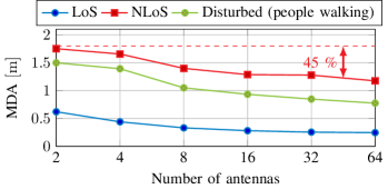
Fig. 7 depicts for the dependency of the MDA on the different amount of antennas. It can be seen that here the LoS case shows only a small improvement by using $64$ antennas instead of 8. In contrast, the robustness of the whole system for the NLoS and “Disturbed Indoor Measurement” case can be significantly improved (over 50% performance gain). Therefore, the same behavior as the simulated case is exhibited. Although in simulations this system could be used with a smaller number of antennas, the effect of hardware impairments and disturbance through the movements/obstacles in the measurement area is reduced by increasing the number of antennas. As those measurements were conducted only within a fixed time interval, an important question remains regarding the overhead to achieve the same performance if the environment changes (e.g. movement) and/or when the hardware impairments become significant.

IV Robustness and time Reproducibility

At first we investigate the performance loss due to changing propagation environments as can be caused by moving obstacles, such as pedestrians or cars. As the main focus of this work is the indoor scenario, we consider “indoor pedestrians” randomly walking through the measurement area. It is important to realize that such obstacles do not only cause a simple signal attenuation, but also may change the propagation scenario from LoS characteristics to NLoS behavior or even shadow several antennas.

Figure 8: Measured: DE CDF for pure LoS and disturbed LoS measurements on the same area.

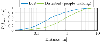
Fig. 8 shows the DE cumulative distribution function (CDF) of different investigations into time reproducibility. For the perfect LoS case, the system achieves a quite reasonable precision in the range of $23\text{\,}\mathrm{cm}$ on an $80\text{\,}\mathrm{m}^{2}$ area. In contrast to the static scenario, in the “Disturbed Indoor Measurement” scenario the performance decreases to around $70\text{\,}\mathrm{cm}$, which is still sufficiently accurate for many practical applications.

IV-A Reproducibility Over Time

Another important property of a practical IPS is the reproducibility over time, i.e., once trained it needs to provide a stable accuracy over time.

Figure 9: Measured: Enhancing time reproducibility via finetuning with different amounts of samples.

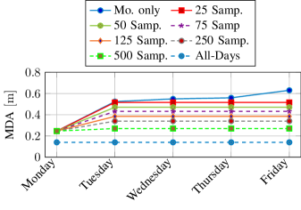
Fig. 9 shows the effect of retraining the NN (that was initially trained on Monday) each day with a different number of points. Although the hardware was turned off and on between the measurement days and the propagation environment may have slightly changed (e.g., due to open doors and windows), it can be seen that even without finetuning the system is still able to achieve a relatively good accuracy of $55\text{\,}\mathrm{cm}$ when inferred on other days. This shows the reproducibility over several time incoherent measurements. To further improve the performance, we propose to measure a small amount of “calibration” points and perform finetuning only on these few points. It can be seen that with 125 samples per day, the loss can be significantly reduced and an accuracy of $40\text{\,}\mathrm{cm}$ is reached. In conclusion, this shows that the proposed NN-based user positioning system is robust to obstacles and, once trained, remains stable over time.

IV-B Pre-training with Simulated Data

We now aim at lowering the amount of required training data and investigate the effects of pre-training. In particular, we compare three different methods:

1. Random initialization of weigths (e.g. Xavier initalization [28]).

2. Pre-training based on the simulated 3GPP model.

3. Pre-training based on a subset of subcarriers, resulting in data augmentation

The intuition behind using only a subset of subcarriers for the initial training is the same as in [29] (data augmentation), where a cropped or rotated image is used to virtually extend the training dataset with similar data in just another presentation. This approach also resembles dropout and results in requiring less samples for achieving an even better overall performance [29].

Figure 10: Measured: Achieved MDA on Monday dataset for different initialization methods and sample distances.

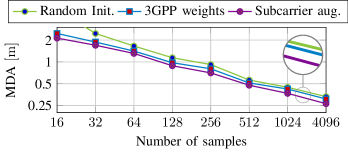
Fig. 10 shows the MDA of the pre-trained model trained on a new propagation environment for different numbers of sample sizes. As expected, the MDA decreases with increasing sample size for all investigated methods. However, even at a high number of samples, there is still a gain of about $10\text{\,}\mathrm{cm}$ for the proposed methods over a randomly initialized NN. We want to emphasize that all data samples obtained by the simulated model or through data augmentation can be considered as free of cost, in contrary to actual measurement data. The NN is able to learn the new scenario with fewer training samples in these pre-trained cases, as the NN can refine its weights according to the propagation environment.

V Conclusions and Outlook

We have shown the practical viability of IPS based on CSI of a Massive MIMO systems even in measured NLoS scenarios with complex propagation environments where most existing solutions would fail. Therefore, a novel NN structure has been proposed based on the idea of an additional feature extraction branch (phase branch), which turned out to improve the performance by a great margin. We showed the robustness of the system for both, moving obstacles in the measurement area as well as in terms of reproducibility over time, i.e., we showcased that, once trained, the system maintains reasonable accuracy over many days. Further, we proposed finetuning and pre-training of the NN to mitigate the effects of varying hardware impairments and changes in the propagation environment which turns out to reduce the number of data points needed for training, resulting in a reduction of the high cost of capturing precise training points.

References

- [1] Microsoft Indoor Localization Competition – IPSN 2018, Microsoft, 2018.
- [2] Z. Iqbal, D. Luo, P. Henry, S. Kazemifar, T. Rozario, Y. Yan, K. D. Westover, W. Lu, D. Nguyen, T. Long, J. Wang, H. Choy, and S. Jiang, “Accurate real time localization tracking in a clinical environment using Bluetooth Low Energy and deep learning,” in PloS one, 2018.
- [3] S. Maranò, W. M. Gifford, H. Wymeersch, and M. Z. Win, “NLOS identification and mitigation for localization based on UWB experimental data,” IEEE JSAC, vol. 28, 2010.
- [4] E. Arias-de Reyna, D. Dardari, P. Closas, and P. Djuric, “Estimation Of Spatial Fields Of Nlos/Los Conditions For Improved Localization In Indoor Environments,” 06 2018, pp. 658–662.
- [5] H. Chen, Y. Zhang, W. Li, X. Tao, and P. Zhang, “ConFi: Convolutional Neural Networks Based Indoor Wi-Fi Localization Using Channel State Information,” IEEE Access, vol. 5, pp. 18 066–18 074, 2017.
- [6] J. Luo and H. Gao, “Deep Belief Networks for Fingerprinting Indoor Localization Using Ultrawideband Technology,” International Journal of Distributed Sensor Networks, vol. 2016, pp. 1–8, 01 2016.
- [7] X. Wang, X. Wang, and S. Mao, “CiFi: Deep convolutional neural networks for indoor localization with 5 GHz Wi-Fi,” in 2017 IEEE International Conference on Communications (ICC), 2017.
- [8] A. Khalajmehrabadi, N. Gatsis, and D. Akopian, “Modern WLAN Fingerprinting Indoor Positioning Methods and Deployment Challenges,” IEEE Communications Surveys & Tutorials, vol. 19, no. 3, Oct. 2017.
- [9] K. S. Kim, S. Lee, and K. Huang, “A scalable deep neural network architecture for multi-building and multi-floor indoor localization based on Wi-Fi fingerprinting,” Big Data Analytics, vol. 3, no. 1, p. 4, Apr 2018.
- [10] P. Bahl and V. N. Padmanabhan, “RADAR: an in-building RF-based user location and tracking system,” in Proceedings IEEE INFOCOM 2000, vol. 2, 2000, pp. 775–784 vol.2.
- [11] V. Savic and E. G. Larsson, “Fingerprinting-Based Positioning in Distributed Massive MIMO Systems,” in 2015 IEEE 82nd Vehicular Technology Conference, Sept 2015, pp. 1–5.
- [12] Z. H. Wu, Y. Han, Y. Chen, and K. J. R. Liu, “A Time-Reversal Paradigm for Indoor Positioning System,” IEEE Transactions on Vehicular Technology, vol. 64, no. 4, pp. 1331–1339, April 2015.
- [13] K. N. R. S. V. Prasad, E. Hossain, and V. K. Bhargava, “Machine Learning Methods for RSS-Based User Positioning in Distributed Massive MIMO,” IEEE Transactions on Wireless Communications, vol. 17, no. 12, pp. 8402–8417, Dec 2018.
- [14] C. Chen, Y. Chen, Y. Han, H. Q. Lai, F. Zhang, and K. J. R. Liu, “Achieving Centimeter-Accuracy Indoor Localization on WiFi Platforms: A Multi-Antenna Approach,” IEEE Internet of Things Journal, vol. 4, no. 1, pp. 122–134, Feb 2017.
- [15] J. Vieira, E. Leitinger, M. Sarajlic, X. Li, and F. Tufvesson, “Deep Convolutional Neural Networks for Massive MIMO Fingerprint-Based Positioning,” ArXiv e-prints, Aug. 2017.
- [16] M. Arnold, S. Dörner, S. Cammerer, and S. ten Brink, “On Deep Learning-based Massive MIMO Indoor User Localization,” SPAWC 2018, 2018.
- [17] A. Decurninge, L. G. Ordóñez, P. Ferrand, G. He, B. Li, W. Zhang, and M. Guillaud, “CSI-based Outdoor Localization for Massive MIMO: Experiments with a Learning Approach,” 2018 15th International Symposium on Wireless Communication Systems (ISWCS), pp. 1–6, 2018.
- [18] N. Ghourchian, M. Allegue-Martínez, and D. Precup, “Real-Time Indoor Localization in Smart Homes Using Semi-Supervised Learning,” in Association for the Advancement of Artificial Intelligence, 2017.
- [19] A. Niitsoo, T. Edelhäußer, E. Eberlein, N. Hadaschik, and C. Mutschler, “A Deep Learning Approach to Position Estimation from Channel Impulse Responses,” Sensors, vol. 19, 03 2019.
- [20] D. Mascharka and E. Manley, “LIPS: Learning Based Indoor Positioning System using mobile phone-based sensors,” in 2016 13th IEEE Annual Consumer Communications Networking Conference (CCNC), 2016.
- [21] T. Feigl, T. Nowak, M. Philippsen, T. Edelhäuβer, and C. Mutschler, “Recurrent Neural Networks on Drifting Time-of-Flight Measurements,” in 2018 International Conference on Indoor Positioning and Indoor Navigation (IPIN), Sep. 2018, pp. 206–212.
- [22] J. H. Emil Björnson and L. Sanguinetti, Massive MIMO Networks: Spectral, Energy, and Hardware Efficiency, 2017.
- [23] S. Jaeckel, L. Raschkowski, K. Borner, and L. Thiele, “QuaDRiGa: A 3-D multi-cell channel model with time evolution for enabling virtual field trials,” IEEE Trans. Antennas Propag., 2014.
- [24] M. Arnold and J. Hoydis and S. ten Brink, “Novel Massive MIMO Channel Sounding Data Applied to Deep Learning-based Indoor Positioning,” SCC 2019, Oct.
- [25] T. O’Shea and J. Hoydis, “An introduction to deep learning for the physical layer,” IEEE Transactions on Cognitive Communications and Networking, vol. 3, no. 4, pp. 563–575, Dec 2017.
- [26] Peter J. Huber, “Robust Estimation of a Location Parameter,” The Annals of Mathematical Statistics, vol. 35, no. 1, pp. 73–101, 1964.
- [27] T. Gruber, S. Cammerer, J. Hoydis, and S. ten Brink, “On deep learning-based channel decoding,” in 2017 51st Annual Conference on Information Sciences and Systems (CISS), March 2017, pp. 1–6.
- [28] X. Glorot and Y. Bengio, “Understanding the difficulty of training deep feedforward neural networks,” in Proceedings of the Thirteenth International Conference on Artificial Intelligence and Statistics, ser. Proceedings of Machine Learning Research, Y. W. Teh and M. Titterington, Eds., vol. 9. Chia Laguna Resort, Sardinia, Italy: PMLR, 13–15 May 2010, pp. 249–256.
- [29] L. Perez and J. Wang, “The effectiveness of data augmentation in image classification using deep learning,” CoRR, vol. abs/1712.04621, 2017.