Radial Prediction Layers

Abstract

For a broad variety of critical applications, it is essential to know how confident a classification prediction is. In this paper, we discuss the drawbacks of softmax to calculate class probabilities and to handle uncertainty in Bayesian neural networks. We introduce a new kind of prediction layer called radial prediction layer (RPL) to overcome these issues. In contrast to the softmax classification, RPL is based on the open-world assumption. Therefore, the class prediction probabilities are much more meaningful to assess the uncertainty concerning the novelty of the input. We show that neural networks with RPLs can be learned in the same way as neural networks using softmax. On a 2D toy data set (spiral data), we demonstrate the fundamental principles and advantages. On the real-world ImageNet data set, we show that the open-world properties are beneficially fulfilled. Additionally, we show that RPLs are less sensible to adversarial attacks on the MNIST data set. Due to its features, we expect RPL to be beneficial in a broad variety of applications, especially in critical environments, such as medicine or autonomous driving.

1 Introduction

Even though deep neural networks are successfully applied to a variety of classification problems (LeCun et al., , 2015), it was shown that the predictions are often fragile and tiny changes in the input could lead to an erroneous classification (Szegedy et al., , 2013; Su et al., , 2019).

Especially in critical environments (e.g., medical applications and autonomous driving), it is necessary to know how confident respectively, how uncertain a (classification) prediction is (Gal, , 2016; Begoli et al., , 2019). Predictive uncertainty can be categorized into two principle types (Kendall and Gal, , 2017). Aleatoric uncertainty captures noise inherent in the observations. Epistemic uncertainty accounts for uncertainty in the model, which can be explained away given enough data. An approach to handle the epistemic uncertainty is the use of Bayesian methods (Hinton and van Camp, , 1993; Blundell et al., , 2015; Gal and Ghahramani, , 2016). Here, we focus on a specific type of epistemic uncertainty which arises if an input at test time is quite different from all of the training examples.

In this paper, we investigate softmax as classification layer in traditional neural networks and Bayesian neural networks and discuss the drawbacks of softmax. We argue that if softmax is used the uncertainty in the weights (epistemic uncertainty) cannot appropriately capture the uncertainty for examples quite different from training data (novel input ${\bf x}$) if the mean field approximation is used, section 3.2.

To overcome this issue, we implemented a simple alternative that we call radial prediction layer (RPL). In contrast to softmax, RPL relies on the open-world assumption (Chen and Liu, , 2018, chapter 5), i.e. the sum of the prediction probabilities for all classes can be significantly smaller than one, e.g., because a test example belongs to a new class which was not in the training data set. This paper describes the fundamental principles and advantages of RPLs on a 2D toy data set (spiral data) for visualization purposes. It demonstrates that the new prediction layer is as flexible as softmax, i.e., it can be used with any type of neural network structure (recurrent, convolutional, etc.) to compute classification probabilities. Neural networks with RPL for the prediction can be trained by a frequentist or by a Bayesian approach with the same optimization criteria as softmax networks.

We further investigated RPLs on the real-world ILSVRC data set (ImageNet (Deng et al., , 2009)) using standard deep neural networks architectures. This paper shows that in such networks, the open-world properties are beneficially fulfilled and similar results can be achieved, as with architectures using softmax. Additionally, it describes that RPLs are less sensible to adversarial attacks on the MNIST data set.

An implementation of RPL based on PyTorch and NumPy is available at:

https://gitlab.com/peroyose/radial_prediction_layers

2 Related Work

Our approach focuses on the uncertainty which results from test data dependent on the novelty of the input. Different techniques exist to detect novel data, see, e.g., Chandola et al., (2009) for a summary. Bishop, (1994) used radial basis functions for density estimation to identify novel examples (input) for neural networks. However, such methods typically do not scale to high dimensional data which are typical for deep learning applications.

Another approach for handling novelty in classification with neural networks is to introduce prediction layers which rely on the open-world assumption (Bendale and Boult, , 2016; Shu et al., , 2017). Bendale and Boult, (2016) propose an extension to softmax, which the authors call openmax. It is based on extreme value theory. To get this open-world extension an additional term in the partition function for a non-class is computed and used. It was also shown that openmax is more robust against adversarial examples (Rozsa et al., , 2017). We show a similar result with our RPLs, see section 5. The approach by Shu et al. is called deep open classification (DOC). DOC builds a 1-vs-rest predication layer based on sigmoids rather than softmax and applies a Gaussian fitting to improve the decision boundaries (Shu et al., , 2017).

3 Softmax and Uncertainty

Usually, classification probabilities are computed by softmax. softmax relies on the closed world assumption, i.e. each data example should be classified to one of the predefined classes $y\in\{1,\dots,K\}$ ($K$ is the number of classes). For the $D$-dimensional input ${\bf x}\in\mathbb{R}^{D}$ the probability that ${\bf x}$ belongs to the class $j$ is denoted by $p(y=j\mid{\bf x})$. With the unnormalized outputs $o_{j}$ of the neural network $p(y=j\mid{\bf x})$ is computed by

$$p(y=j\mid{\bf x})=\frac{\exp(o_{j})}{\sum_{i}\exp(o_{i})}$$ (1)

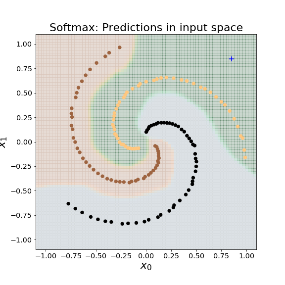
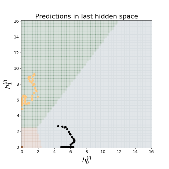
By definition of softmax, the predicted probabilities for all classes sum up to one. As we discuss later, the closed world assumption is problematic if at test time an input ${\bf x}$ is quite different from all the training examples. We call such inputs "novel" or “far away” from the training data, for an example see the blue data point in figure 1. Formally, a data point ${\bf x}$ is "novel" if the probability for sampling such a data point ${\bf x}$ as a training example is approximate zero, i.e., $p_{train}({\bf x})\approx 0$.

Figure 1: On the left side the spiral data set and a typical prediction by a neural network with a softmax layer is shown. The blue cross represents a test example which is “far away” from the training data. For such test examples the uncertainty of the prediction should be very high. However, a high probability for the yellow class is predicted by softmax. On the right side the last hidden layer before the softmax layer is shown. The network maps the data into this layer such that the data is linear separable. Due to the use of ReLU non-linearities only the positive quadrant is accessible (and shown here).

3.1 Traditional Neural Networks

We use the spiral data set for illustration purposes. A fully connected feed forward neural network maps the input ${\bf x}$ in each layer to a new representation ${\bf h}^{(i)}$, $i$ being the layer index. With softmax the representation in the last hidden layer ${\bf h}^{(l)}$ has to be linear separable w.r.t. the different classes. So the neural network learns such a mapping ${\bf x}\rightarrow{\bf h}^{(l)}$, see figure 1(right). That corresponds to complex decision boundaries in the input space, see figure 1 (left).

3.2 Bayesian Neural Networks

Scalable Bayesian neural networks rely on the mean field approximation and can, e.g., be trained by the backpropagation algorithm minimizing the evidence lower bound (ELBO) in a variational approach (Blundell et al., , 2015), see also supplementary material. However, different approximation techniques for learning and prediction for Bayesian networks exist (Hinton and van Camp, , 1993; Blundell et al., , 2015; Gal and Ghahramani, , 2016). As well as traditional neural networks, Bayesian neural networks have typically a softmax layer to compute the class probabilities.

In a Bayesian neural network, the mapping from the input to the last hidden layer ${\bf x}\rightarrow{\bf h}^{(l)}$ is not deterministic. ${\bf h}^{(l)}({\bf x})$ is represented by a probability density function $p({\bf h}^{(l)}({\bf x}))$ for a fixed input ${\bf x}$. That is part of the uncertainty of the model (epistemological uncertainty). This uncertainty is mediated by the probability distribution of the weights. Additionally, there is a (probabilistic) mapping from ${\bf h}^{(l)}$ to the logit output ${\bf o}$ which is also part of the model uncertainty. In the mean field approximation these uncertainties are independent. In other words, the probability density factorizes with a term for each unit (and therefore also layer). The probabilistic decision boundaries of the softmax layer are independent of the probabilistic mapping ${\bf x}\rightarrow{\bf h}^{(l)}$.

Figure 2: Stochastic mapping from an input data example by different samples of a Bayesian neural network. In the inner plot the prediction distribution of the most-probable class for the corresponding data point is shown. On the left side for a training example. On the right side for the “far away” test example (blue cross of figure 1). Depending on the stochasticity of the training, e.g. the weight initialization, this can result in quite high prediction probabilities of the test example.

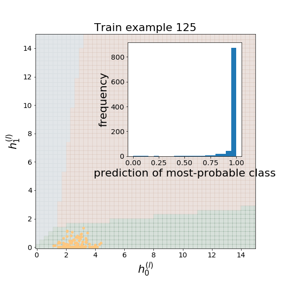
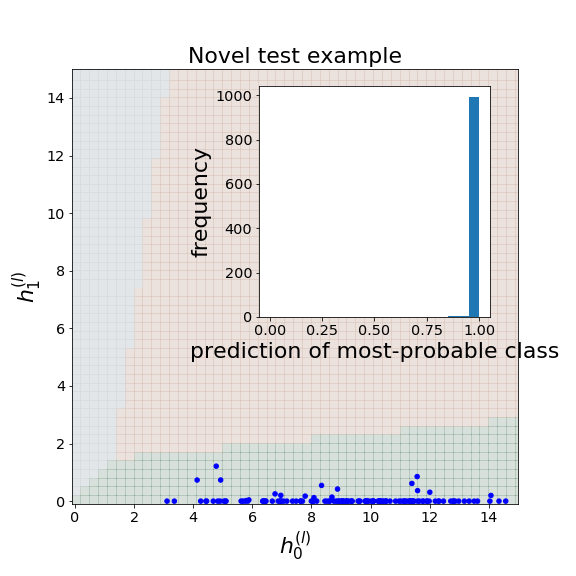
In practice, samples of the weights are drawn which corresponds to a sample of the Bayesian network . If a training example is mapped (${\bf x}\rightarrow{\bf h}^{(l)}$) by different samples of a Bayesian network it must be mapped in the same region. Because of the independence, there cannot be any correlation which adapts the decision boundaries for the specific sample of the Bayesian network. (On the spiral data set,) this results in quite the same decision boundaries for different samples of the Bayesian network (for a figure see supplementary material). The mapping ${\bf x}\rightarrow{\bf h}^{(l)}$ for the training data must be such that the correct class prediction is mainly fulfilled. It is mapped mostly on the correct side of the decision boundaries. So, an input ${\bf x}$ is mapped in nearby regions. The same holds if novel data is mapped in the last hidden layer. If the probabilistic mapping ${\bf x}\rightarrow{\bf h}^{(l)}$ puts the data in a region where high probabilities by softmax logistic regression are assigned then the uncertainty of the prediction seems to be very low. This is not a wanted behaviour, see figure 2(left) . So, the combination of the softmax model and the mean field approximation can result in strong underestimated (prediction) uncertainties.

4 Radial Prediction Layers

A radial prediction layer is the last layer of a neural network. As in softmax networks the input ${\bf x}$ is mapped into an output (vector) ${\bf o}={\bf o}({\bf x})$. In case of RPLs, we call the corresponding vector space the RPL-(vector)-space. The mapping from the last hidden layer representation ${\bf h}^{(l)}$ to ${\bf o}$ is done by a pure affine transformation without a non-linear activation function. Therefore, the full RPL space is accessible and not e.g., only the positive part (if ReLU would be used).

In the RPL-space, there is a prototype vector ${\bf p}_{j}$ for each class $j$. The predicted class probability for an input feature vector ${\bf x}$ is given by $p(y=j\mid{\bf x})=\exp(-\beta d_{j}({\bf x}))$, with $d_{j}({\bf x})$ being the distance of ${\bf o}({\bf x})$ to the prototype vector ${\bf p}_{j}$. $\beta>0$ is a hyperparameter. As a metric, we use the Euclidean distance, but in principle other distances are possible without restricting the general idea. So with the prototype vector ${\bf p}_{j}$ for class $j$ in the RPL-space and $\mid\mid.\mid\mid_{2}$ for the notation of the $\ell$2-norm the distance is

$$d_{j}({\bf x})=\mid\mid{\bf p}_{j}-{\bf o}({\bf x})\mid\mid_{2}$$ (2)

If an input is mapped exactly to a prototype then the probability that it belongs to the corresponding class is $\exp(0)=1$. With increased distance the probability goes exponentially towards zero.

We put the prototypes on the axes of the coordinate system of the RPL-space ${\bf p}_{j}=a{\bf e}_{j}$. The vectors ${\bf e}_{j}$ form an orthonormal basis of the coordinate system of the RPL space. In neural network terminology, ${\bf e}_{j}$ is equivalent to a one-hot encoded state representation in the RPL-space. $a$ is the distance of all prototypes to the origin. The distance $c$ between the prototypes is given by the Pythagorean theorem: $c=\sqrt{2}a$.

The open-world assumption demands that the sum of the predicted probabilities of all classes must be equal or smaller than one, $\sum_{k}p(y=k\mid{\bf x};{\bf w})\leq 1$. If an input is now mapped exactly to a prototype $j$ then the predicted class probabilities for the other classes $k\neq j$ must be zero. This could be realized by setting the probability $p(y=k\mid{\bf x};{\bf w})$ to zero if the distance is greater than a threshold $c^{\prime}\leq c$:

$$p(y=k\mid{\bf x};{\bf w})=\begin{cases}\exp\left(-\beta d_{k}({\bf x})\right)&\text{if }d_{k}({\bf x})<c^{\prime}\\ 0&\text{else}\end{cases}$$ (3)

In practice, we just set the hyperparameters $a$ and $\beta$ such that $\exp\left(-\beta c\right)$ has a very small value.

4.1 Learning

Without considering regularization, the weights ${\bf w}$ of a neural network are typically learned with a train data set $\mathcal{D}_{train}=\{\left({\bf x}^{(1)},y^{(1)}\right),\left({\bf x}^{(2)},y^{(2)}\right),\dots,\left({\bf x}^{(m)},y^{(m)}\right)$ by minimizing the negative log-likelihood $-\ell({\bf w})=-\sum_{i}\log p(y^{(i)}\mid{\bf x}^{(i)};{\bf w})$.

Using the threshold rule 3 for learning would be problematic. If the distance to the target prototype is greater then $c^{\prime}$ this would result in a zero gradient. So, during learning we just used $p(y=k\mid{\bf x};{\bf w})=\exp\left(-\beta d_{k}({\bf x})\right)$. The corresponding (negative log likelihood) loss for RPL of an example $i$ with target class $k$ is

$$-\log p(y^{(i)}=k\mid{\bf x}^{(i)};{\bf w})=\beta d_{k}({\bf x})=\beta\;\mid\mid{\bf o}({\bf x}^{(i)})-{\bf p}_{k}\mid\mid_{2}$$ (4)

Minimizing the negative log-likelihood is equivalent to minimizing the distance to the target prototype. The hyperparameter $\beta$ just scales the log-likelihood and can therefore be neglected in the minimization.

4.2 Example: Spiral Data

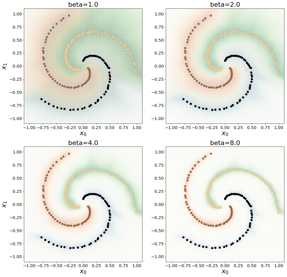
In figure 3 (right) typical predictions for the spiral data set are shown with $a=1$. For larger $\beta$-values, only on the spiral manifolds the prediction probabilities for the corresponding classes are substantially greater than zero. In all other regions of the input space the prediction for all classes is very low.

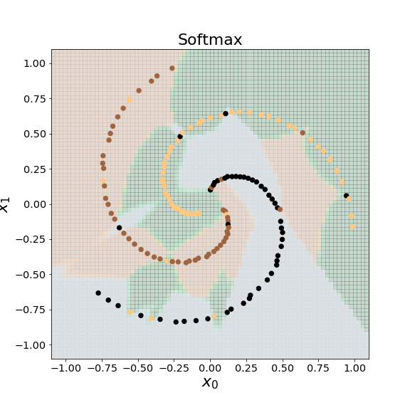
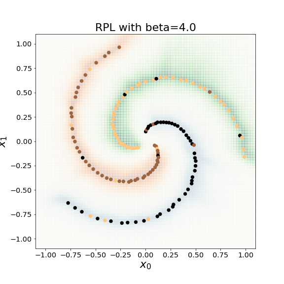
A result of the spiral data set with noisy labels $t$ is shown in figure 4 for softmax and RPL.

Figure 3: Predictions for different values of the hyperparameter $\beta$ on the spiral data set ($a=1$). With increased value of $\beta$ the predictions with high class probabilities become more and more restricted to the narrow spiral manifolds.

Figure 4: Prediction with noise (10%), i.e. 10% of the data points have a random label. High capacity networks with softmax show strong overfitting behaviour (left plot). Surprisingly, high capacity RPL networks seem to be quite robust against overfitting (right plot) with similar predictions as in the no-noise case.

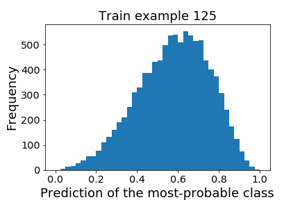
RPL layers can also be used in Bayesian neural networks. We trained such networks with the spiral data set. In figure 5 are the prediction probability distributions of a training and a (novel) test example shown.

Figure 5: Probability distributions of Bayesian neural networks with RPL analog to figure 2 (inner plots) for the same training (left) and test (right) example. The distributions are much broader and more meaningful as with softmax.

4.3 Example: MNIST

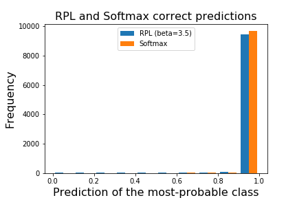
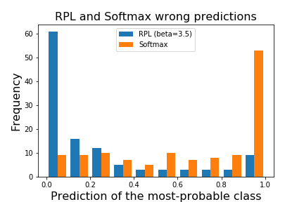
We trained both variants without tuning of any hyperparameters (no regularization) on the MNIST train set with a convolutional neural network. Both variants, softmax, and RPL attained a similar accuracy of approximated $0.988$. The histograms of the predicted most-probable class for the correct and wrong predictions are shown in figure 6. Sometimes, the predicted class probabilities are used as confidence measures. With softmax, such confidences are even for wrong predictions quite high. In contrast, with RPL wrong predictions have mostly a quite low predicted probability ( 6, right).

Figure 6: Histograms of the frequencies of correct predictions and wrong predictions (max of the class probabilities) of a neural network with RPL and Softmax as classification layer for the MNIST test data set. In the RPL case, for the wrong predictions the probability is mostly quite low.

4.4 Example: ILSVRC Data

We explored RPLs on the ILSVRC dataset (ImageNet) (Deng et al., , 2009) to verify that the approach is applicable to real-world data and deep neural network architectures. We examined several architectures (Krizhevsky et al., , 2012; Simonyan and Zisserman, , 2014; He et al., , 2016), and all could be trained with RPLs. However, this paper focuses on the VGG network (Simonyan and Zisserman, , 2014), which we have studied most intently. We trained the network multiple times with one training setup in two variations: pre-trained (reinitialize fully connected layers) and from scratch (reinitialize all parameters). Additionally, we trained a network on a subset of the ImageNet data, and used the removed classes as novel data in the test phase. A detailed description of network architectures, training setups and hyperparameter is provided in the supplementary material.

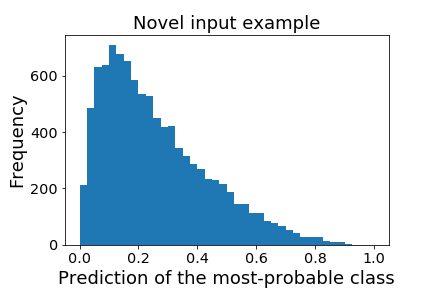
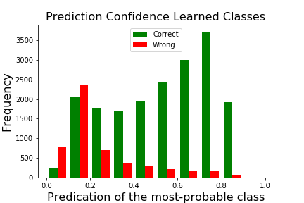
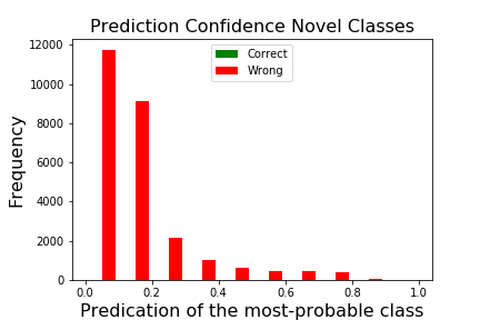
The experiments show that similar accuracies can be achieved with RPLs in deep network architectures compared to softmax. In this statement, we assume an error value(doubled corrected sample standard deviation) of X.Y. Table 1 summarizes the accuracies and compares them to the results achieved by (Simonyan and Zisserman, , 2014)(Table 3 - ConvNet performance at a single test scale) with softmax. Figure 7 presents the results for the network trained on an ImageNet subset. The network was validated on classes used during training and is quite confident in the decisions if we use the predicted class probabilities as confidence measure (right). In contrast, the prediction confidence for novel data is quite low (left) as expected from the open-world property of the RPL.

Table 1: Achived accuracies for the MNIST and ImageNet datasets. For Imagenet the trained variations VGG (A), (B) and (C) are compared with respect to top-1 and top-5 accuracy. VGG(A) is a pre-trained network with reinitialized fully connected layers using RPL. VGG(B) is a fully reinitialized network using RPL. VGG(C) is the original network reported in (Simonyan and Zisserman, , 2014).

	MNIST		VGG (A)	VGG (B)	VGG  (Simonyan and Zisserman, , 2014)
	Softmax	RPL	RPL	RPL	Softmax
Acc (top-1)	0.9878	0.9880	76.1	78.7	74.5
Acc (top-5)	-	-	91.4	90.0	92.0

Figure 7: Histogram of the frequencies of correct predictions and wrong predictions of a VGG network with RPL for the validation data (right) and novel data (left) are shown (ImageNet). The network was trained on a subset. Data removed from the training set was used as novel data (novel classes). For the wrong predictions (max of the class probabilities) the probability is mostly quite low for RPL. Note, that by increasing the hyperparameter $\beta$ the distributions could be shifted to the left side.

5 Adversarial Examples

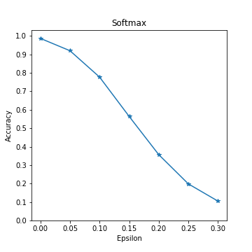
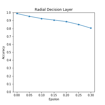
We also investigated how prone RPL is against Fast Gradient Sign Attack (FGSM) (Goodfellow et al., , 2014) in comparison with softmax on the MNIST dataset. In FGSM the input is additively perturbed in the direction that maximizes the loss. This pushes down the predicted probability of the corresponding class. The strength of the perturbation is controlled by a parameter $\epsilon$ . With increased $\epsilon$ the accuracy of the test data set drops and more and more test examples are classified incorrectly, see figure 8. From the figure can be seen that RPL is much less prone to FGSM.

Figure 8: Accuracy of the MNIST test data set for different levels of adversarial perturbation (epsilon). On the left for a neural network with a softmax prediction layer and on the right for a neural network with RPL.

6 Conclusion

In this paper, we describe the drawbacks of softmax in the context of uncertainty on a novel input ${\bf x}$. We proposed RPL as an alternative to softmax, which is based on the open-world assumption. We showed that RPL has beneficial properties for handling the uncertainty concerning the novelty of the input. For application where such a feature is useful, RPL could be an alternative to softmax. We demonstrated that common deep neural network architectures can be trained with RPLs without many modifications. Further research is necessary to understand all the implications of the usage of RPL in depth.

RPL can be used in Bayesian neural networks to combine the desirable properties, e.g., for handling uncertainty and preventing overfitting. We also showed that RPL is less prone to adversarial examples. This can be explained with the open-world assumption inherent in RPL(Rozsa et al., , 2017).

Acknowledgments

The authors acknowledge the financial support by the Federal Ministry of Education and Research of Germany (BMBF) in the project deep.Health (project number 13FH770IX6).

References

- Begoli et al., [2019] Begoli, E., Bhattacharya, T., and Kusnezov, D. (2019). The need for uncertainty quantification in machine-assisted medical decision making. Nature Machine Intelligence, pages 20–23.
- Bendale and Boult, [2016] Bendale, A. and Boult, T. E. (2016). Towards open set deep networks. In 2016 IEEE Conference on Computer Vision and Pattern Recognition, CVPR 2016, Las Vegas, NV, USA, June 27-30, 2016, pages 1563–1572. IEEE Computer Society.
- Bishop, [1994] Bishop, C. (1994). Novelty detection and neural network validation. Vision, Image and Signal Processing, IEE Proceedings -, 141:217 – 222.
- Blundell et al., [2015] Blundell, C., Cornebise, J., Kavukcuoglu, K., and Wierstra, D. (2015). Weight uncertainty in neural networks. In Proceedings of the 32nd International Conference on International Conference on Machine Learning - Volume 37, ICML’15, pages 1613–1622. JMLR.org.
- Chandola et al., [2009] Chandola, V., Banerjee, A., and Kumar, V. (2009). Anomaly detection: A survey. ACM Comput. Surv., 41(3):15:1–15:58.
- Chen and Liu, [2018] Chen, Z. and Liu, B. (2018). Lifelong Machine Learning, Second Edition. Synthesis Lectures on Artificial Intelligence and Machine Learning. Morgan & Claypool Publishers.
- Deng et al., [2009] Deng, J., Dong, W., Socher, R., Li, L.-J., Li, K., and Fei-Fei, L. (2009). ImageNet: A Large-Scale Hierarchical Image Database. In CVPR09.
- Gal, [2016] Gal, Y. (2016). Uncertainty in Deep Learning. PhD thesis, University of Cambridge.
- Gal and Ghahramani, [2016] Gal, Y. and Ghahramani, Z. (2016). Dropout as a bayesian approximation: Representing model uncertainty in deep learning. In Proceedings of the 33rd International Conference on International Conference on Machine Learning - Volume 48, ICML’16, pages 1050–1059. JMLR.org.
- Goodfellow et al., [2014] Goodfellow, I., Shlens, J., and Szegedy, C. (2014). Explaining and harnessing adversarial examples. arXiv 1412.6572.
- He et al., [2016] He, K., Zhang, X., Ren, S., and Sun, J. (2016). Deep residual learning for image recognition. In Proceedings of the IEEE conference on computer vision and pattern recognition, pages 770–778.
- Hinton and van Camp, [1993] Hinton, G. E. and van Camp, D. (1993). Keeping the neural networks simple by minimizing the description length of the weights. In Proceedings of the Sixth Annual Conference on Computational Learning Theory, COLT ’93, pages 5–13, New York, NY, USA. ACM.
- Kendall and Gal, [2017] Kendall, A. and Gal, Y. (2017). What uncertainties do we need in bayesian deep learning for computer vision? In Guyon, I., Luxburg, U. V., Bengio, S., Wallach, H., Fergus, R., Vishwanathan, S., and Garnett, R., editors, Advances in Neural Information Processing Systems 30, pages 5574–5584. Curran Associates, Inc.
- Krizhevsky et al., [2012] Krizhevsky, A., Sutskever, I., and Hinton, G. E. (2012). Imagenet classification with deep convolutional neural networks. In Advances in neural information processing systems, pages 1097–1105.
- LeCun et al., [2015] LeCun, Y., Bengio, Y., and Hinton, G. (2015). Deep learning. Nature, 521(7553):436.
- Rozsa et al., [2017] Rozsa, A., Günther, M., and Boult, T. E. (2017). Adversarial robustness: Softmax versus openmax. In British Machine Vision Conference 2017, BMVC 2017, London, UK, September 4-7, 2017. BMVA Press.
- Shu et al., [2017] Shu, L., Xu, H., and Liu, B. (2017). DOC: Deep open classification of text documents. In Proceedings of the 2017 Conference on Empirical Methods in Natural Language Processing, pages 2911–2916, Copenhagen, Denmark. Association for Computational Linguistics.
- Simonyan and Zisserman, [2014] Simonyan, K. and Zisserman, A. (2014). Very deep convolutional networks for large-scale image recognition. arXiv preprint arXiv:1409.1556.
- Su et al., [2019] Su, J., Vargas, D. V., and Sakurai, K. (2019). One pixel attack for fooling deep neural networks. IEEE Transactions on Evolutionary Computation.
- Szegedy et al., [2013] Szegedy, C., Zaremba, W., Sutskever, I., Bruna, J., Erhan, D., Goodfellow, I., and Fergus, R. (2013). Intriguing properties of neural networks. arXiv preprint arXiv:1312.6199.