Learning step sizes for unfolded sparse coding

Abstract

Sparse coding is typically solved by iterative optimization techniques, such as the Iterative Shrinkage-Thresholding Algorithm (ISTA). Unfolding and learning weights of ISTA using neural networks is a practical way to accelerate estimation. In this paper, we study the selection of adapted step sizes for ISTA. We show that a simple step size strategy can improve the convergence rate of ISTA by leveraging the sparsity of the iterates. However, it is impractical in most large-scale applications. Therefore, we propose a network architecture where only the step sizes of ISTA are learned. We demonstrate that for a large class of unfolded algorithms, if the algorithm converges to the solution of the Lasso, its last layers correspond to ISTA with learned step sizes. Experiments show that our method is competitive with state-of-the-art networks when the solutions are sparse enough.

1 Introduction

The resolution of convex optimization problems by iterative algorithms has become a key part of machine learning and signal processing pipelines. Amongst these problems, special attention has been devoted to the Lasso (Tibshirani, 1996), due to the attractive sparsity properties of its solution (see Hastie et al. 2015 for an extensive review). For a given input $x\in\mathbb{R}^{n}~{},$ a dictionary $D\in\mathbb{R}^{n\times m}$ and a regularization parameter $\lambda>0~{},$ the Lasso problem is

$$z^{*}(x)\in\operatorname*{arg\,min}_{z\in\mathbb{R}^{m}}F_{x}(z)\quad\textrm{with}\quad F_{x}(z)\triangleq\frac{1}{2}\|x-Dz\|^{2}+\lambda\|z\|_{1}\enspace.$$ (1)

A variety of algorithms exist to solve Problem (1), e.g. proximal coordinate descent (Tseng, 2001; Friedman et al., 2007), Least Angle Regression (Efron et al., 2004) or proximal splitting methods (Combettes and Bauschke, 2011). The focus of this paper is on the Iterative Shrinkage-Thresholding Algorithm (ISTA, Daubechies et al. 2004), which is a proximal-gradient method applied to Problem (1). ISTA starts from $z^{(0)}=0$ and iterates

$$z^{(t+1)}=\operatorname{ST}\left(z^{(t)}-\frac{1}{L}D^{\top}(Dz^{(t)}-x),\frac{\lambda}{L}\right)\enspace,$$ (2)

where $\operatorname{ST}$ is the soft-thresholding operator defined as $\operatorname{ST}(x,u)\triangleq\text{sign}(x)\max(|x|-u,0)~{},$ and $L$ is the greatest eigenvalue of $D^{\top}D~{}.$ In the general case, ISTA converges at rate $1/t~{},$ which can be improved to the optimal rate $1/t^{2}$ (Nesterov, 1983). However, this optimality stands in the worst possible case, and linear rates are achievable in practice (Liang et al., 2014).

A popular line of research to improve the speed of Lasso solvers is to try to identify the support of $z^{*}~{},$ in order to diminish the size of the optimization problem (El Ghaoui et al., 2012; Ndiaye et al., 2017; Johnson and Guestrin, 2015; Massias et al., 2018). Once the support is identified, larger steps can also be taken, leading to improved rates for first order algorithms (Liang et al., 2014; Poon et al., 2018; Sun et al., 2019).

However, these techniques only consider the case where a single Lasso problem is solved. When one wants to solve the Lasso for many samples $\{x^{i}\}_{i=1}^{N}$ – e.g. in dictionary learning (Olshausen and Field, 1997) – it is proposed by Gregor and Le Cun (2010) to learn a $T$-layers neural network of parameters $\Theta~{},$ $\Phi_{\Theta}:\mathbb{R}^{n}\rightarrow\mathbb{R}^{m}$ such that $\Phi_{\Theta}(x)\simeq z^{*}(x)~{}.$ This Learned-ISTA (LISTA) algorithm yields better solution estimates than ISTA on new samples for the same number of iterations/layers. This idea has led to a profusion of literature (summarized in Table A.1 in appendix). Recently, it has been hinted by Zhang and Ghanem (2018); Ito et al. (2018); Liu et al. (2019) that only a few well-chosen parameters can be learned while retaining the performances of LISTA.

In this article, we study strategies for LISTA where only step sizes are learned. In Section 3, we propose Oracle-ISTA, an analytic strategy to obtain larger step sizes in ISTA. We show that the proposed algorithm’s convergence rate can be much better than that of ISTA. However, it requires computing a large number of Lipschitz constants which is a burden in high dimension. This motivates the introduction of Step-LISTA (SLISTA) networks in Section 4, where only a step size parameter is learned per layer. As a theoretical justification, we show in Theorem 4.4 that the last layers of any deep LISTA network converging on the Lasso must correspond to ISTA iterations with learned step sizes. We validate the soundness of this approach with numerical experiments in Section 5.

2 Notation and Framework

Notation

The $\ell_{2}$ norm on $\mathbb{R}^{n}$ is $\|\cdot\|$. For $p\in[1,\infty]~{},$ $\|\cdot\|_{p}$ is the $\ell_{p}$ norm. The Frobenius matrix norm is $\|M\|_{F}$. The identity matrix of size $m$ is $\operatorname{Id}_{m}~{}.$ $\operatorname{ST}$ is the soft-thresholding operator. Iterations are denoted $z^{(t)}~{}.$ $\lambda>0$ is the regularization parameter. The Lasso cost function is $F_{x}~{}.$ $\psi_{\alpha}(z,x)$ is one iteration of ISTA with step $\alpha$: $\psi_{\alpha}(z,x)=\operatorname{ST}(z-\alpha D^{\top}(Dz-x),\alpha\lambda)~{}.$ $\phi_{\theta}(z,x)$ is one iteration of a LISTA layer with parameters $\theta=(W,\alpha,\beta)$: $\phi_{\theta}(z,x)=\operatorname{ST}(z-\alpha W^{\top}(Dz-x),\beta\lambda)~{}.$

The set of integers between 1 and $m$ is $\llbracket 1,m\rrbracket~{}.$ Given $z\in\mathbb{R}^{m}~{},$ the support is $\operatorname*{supp}(z)=\{j\in\llbracket 1,m\rrbracket:z_{j}\neq 0\}\subset\llbracket 1,m\rrbracket~{}.$ For $S\subset\llbracket 0,m\rrbracket$, $D_{S}\in~\mathbb{R}^{n\times m}$ is the matrix containing the columns of $D$ indexed by $S$. We denote $L_{S},$ the greatest eigenvalue of $D_{S}^{\top}D_{S}$. The equicorrelation set is $E=\{j\in\llbracket 1,m\rrbracket:|D_{j}^{\top}(Dz^{*}-x)|=\lambda\}$. The equiregularization set is $\mathcal{B}_{\infty}=\{x\in\mathbb{R}^{n}:\|D^{\top}x\|_{\infty}=1\}$. Neural networks parameters are between brackets, e.g.  $\Theta=\{\alpha^{(t)},\beta^{(t)}\}_{t=0}^{T-1}~{}.$ The sign function is $\operatorname*{sign}(x)=1$ if $x>0$, $-1$ if $x<0$ and $0$ is $x=0~{}.$

Framework

This paragraph recalls some properties of the Lasso. 2.1 gives the first-order optimality conditions for the Lasso.

Lemma 2.1 (Optimality for the Lasso).

The Karush-Kuhn-Tucker (KKT) conditions read

$$z^{*}\in\operatorname*{arg\,min}F_{x}\Leftrightarrow\forall j\in\llbracket 1,m\rrbracket,D_{j}^{\top}(x-Dz^{*})\in\lambda\partial|z^{*}_{j}|=\begin{cases}\begin{aligned} &\{\lambda\operatorname*{sign}z^{*}_{j}\},&\mathrm{if\,}z^{*}_{j}\neq 0\enspace,\\ &[-\lambda,\lambda],&\mathrm{if\,}z^{*}_{j}=0\enspace.\end{aligned}\end{cases}$$ (3)

Defining $\lambda_{\max}\triangleq\|D^{\top}x\|_{\infty}~{},$ it holds $\operatorname*{arg\,min}F_{x}=\{0\}\Leftrightarrow\lambda\geq\lambda_{\max}~{}.$ For some results in Section 3, we will need the following assumption on the dictionary $D$:

Assumption 2.2 (Uniqueness assumption).

$D$ is such that the solution of Problem (1) is unique for all $\lambda$ and $x$ i.e. $\operatorname*{arg\,min}F_{x}=\{z^{*}\}~{}.$

2.2 may seem stringent since whenever $m>n~{},$ $F_{x}$ is not strictly convex. However, it was shown in Tibshirani (2013, Lemma 4) – with earlier results from Rosset et al. 2004 – that if $D$ is sampled from a continuous distribution, 2.2 holds for $D$ with probability one.

Definition 2.3 (Equicorrelation set).

The KKT conditions motivate the introduction of the equicorrelation set $E\triangleq\{j\in\llbracket 1,m\rrbracket:|D_{j}^{\top}(Dz^{*}-x)|=\lambda\}~{},$ since $j\notin E\implies z^{*}_{j}=0~{},$ i.e. $E$ contains the support of any solution $z^{*}~{}.$

When 2.2 holds, we have $E=\operatorname*{supp}(z^{*})$ (Tibshirani, 2013, Lemma 16).

We consider samples $x$ in the equiregularization set

$$\mathcal{B}_{\infty}\triangleq\{x\in\mathbb{R}^{n}:\|D^{\top}x\|_{\infty}=1\}\enspace,$$ (4)

which is the set of $x$ such that $\lambda_{\text{max}}(x)=1~{}.$ Therefore, when $\lambda\geq 1~{},$ the solution is $z^{*}(x)=0$ for all $x\in\mathcal{B}_{\infty}~{},$ and when $\lambda<1~{},$ $z^{*}(x)\neq 0$ for all $x\in\mathcal{B}_{\infty}~{}.$ For this reason, we assume $0<\lambda<1$ in the following.

3 Better step sizes for ISTA

The Lasso objective is the sum of a $L$-smooth function, $\frac{1}{2}\|x-D\cdot\|^{2}~{},$ and a function with an explicit proximal operator, $\lambda\|\cdot\|_{1}~{}.$ Proximal gradient descent for this problem, with the sequence of step sizes $(\alpha^{(t)})$ consists in iterating

$$z^{(t+1)}=\operatorname{ST}\left(z^{(t)}-\alpha^{(t)}D^{\top}(Dz^{(t)}-x),\lambda\alpha^{(t)}\right)\enspace.$$ (5)

ISTA follows these iterations with a constant step size $\alpha^{(t)}=1/L~{}.$ In the following, denote $\psi_{\alpha}(z,x)\triangleq\operatorname{ST}(z-\alpha D^{\top}(Dz^{(t)}-x),\alpha\lambda)$. One iteration of ISTA can be cast as a majorization-minimization step (Beck and Teboulle, 2009). Indeed, for all $z\in\mathbb{R}^{m}~{},$

$$F_{x}(z) =\tfrac{1}{2}\|x-Dz^{(t)}\|^{2}+(z-z^{(t)})^{\top}D^{\top}(Dz^{(t)}-x)+\tfrac{1}{2}\|D(z-z^{(t)})\|^{2}+\lambda\|z\|_{1}$$ (6)

$$\leq\underbrace{\tfrac{1}{2}\|x-Dz^{(t)}\|^{2}+(z-z^{(t)})^{\top}D^{\top}(Dz^{(t)}-x)+\tfrac{L}{2}\|z-z^{(t)}\|^{2}+\lambda\|z\|_{1}}_{\displaystyle\triangleq Q_{x,L}(z,z^{(t)})}\enspace,$$ (7)

where we have used the inequality $(z-z^{(t)})^{\top}D^{\top}D(z-z^{(t)})\leq L\|z-z^{(t)}\|^{2}~{}.$ The minimizer of $Q_{x,L}(\cdot,z^{(t)})$ is $\psi_{1/L}(z^{(t)},x)$, which is the next ISTA step.

Oracle-ISTA: an accelerated ISTA with larger step sizes

Since the iterates are sparse, this approach can be refined. For $S\subset\llbracket 1,m\rrbracket~{},$ let us define the $S$-smoothness of $D$ as

$$L_{S}\triangleq\max_{z}z^{\top}D^{\top}Dz,\enspace\text{s.t.}\enspace\|z\|=1\text{ and supp}(z)\subset S\enspace,$$ (8)

with the convention $L_{\emptyset}=L~{}.$ Note that $L_{S}$ is the greatest eigenvalue of $D_{S}^{\top}D_{S}$ where $D_{S}\in\mathbb{R}^{n\times|S|}$ is the columns of $D$ indexed by $S~{}.$ For all $S~{},$ $L_{S}\leq L~{},$ since $L$ is the solution of Equation 8 without support constraint. Assume $\operatorname*{supp}(z^{(t)})\subset S~{}.$ Combining Equations 6 and 8, we have

$$\forall z\enspace\text{s.t.}\enspace\operatorname*{supp}(z)\subset S,\enspace F_{x}(z)\leq Q_{x,L_{S}}(z,z^{(t)})\enspace.$$ (9)

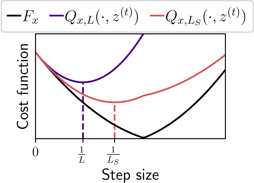
The minimizer of the r.h.s is $z=\psi_{{1}/{L_{S}}}(z^{(t)},x)~{}.$ Furthermore, the r.h.s. is a tighter upper bound than the one given in Equation 7 (see illustration in Figure 1). Therefore, using $z^{(t+1)}=\psi_{{1}/{L_{S}}}(z^{(t)},x)$ minimizes a tighter upper bound, provided that the following condition holds

$$\operatorname*{supp}(z^{(t+1)})\subset S~{}.$$

Figure 1: Majorization illustration. If $z^{(t)}$ has support $S~{},$ $Q_{x,L_{S}}(\cdot,z^{(t)})$ is a tighter upper bound of $F_{x}$ than $Q_{x,L}(\cdot,z^{(t)})$ on the set of points of support $S~{}.$

Input: Dictionary $D~{},$ target $x~{},$ number of iterations $T$

$z^{(0)}=0$

for $t=0,\ldots,T-1$ do

       Compute $S=\operatorname*{supp}(z^{(t)})$ and $L_{S}$ using an oracle ;

       Set $y^{(t+1)}=\psi_{{1}/{L_{S}}}(z^{(t)},x)$ ;

       if Section 3 : $\operatorname*{supp}(y^{(t+1)})\subset S$  then  Set $z^{(t+1)}=y^{(t+1)}$ ;

       else  Set $z^{(t+1)}=\psi_{{1}/{L}}(z^{(t)},x)$ ;

      

Output: Sparse code $z^{(T)}$

Algorithm 1 Oracle-ISTA (OISTA) with larger step sizes

Oracle-ISTA (OISTA) is an accelerated version of ISTA which leverages the sparsity of the iterates in order to use larger step sizes. The method is summarized in Algorithm 1. OISTA computes $y^{(t+1)}=\psi_{1/L_{s}}(z^{(t)},x)~{},$ using the larger step size $1/L_{S}~{},$ and checks if it satisfies the support Section 3. When the condition is satisfied, the step can be safely accepted. In particular Equation 9 yields $F_{x}(y^{(t+1)})\leq F_{x}(z^{(t)})~{}.$ Otherwise, the algorithm falls back to the regular ISTA iteration with the smaller step size. Hence, each iteration of the algorithm is guaranteed to decrease $F_{x}~{}.$ The following proposition shows that OISTA converges in iterates, achieves finite support identification, and eventually reaches a safe regime where Section 3 is always true.

Proposition 3.1 (Convergence, finite-time support identification and safe regime).

When 2.2 holds, the sequence $(z^{(t)})$ generated by the algorithm converges to $z^{*}=\operatorname*{arg\,min}F_{x}~{}.$

Further, there exists an iteration $T^{*}$ such that for $t\geq T^{*}~{},$ $\operatorname*{supp}(z^{(t)})=\operatorname*{supp}(z^{*})\triangleq S^{*}$ and Section 3 is always statisfied.

Sketch of proof (full proof in Subsection B.1).

Using Zangwill’s global convergence theorem (Zangwill, 1969), we show that all accumulation points of $(z^{(t)})$ are solutions of Lasso. Since the solution is assumed unique, $(z^{(t)})$ converges to $z^{*}~{}.$ Then, we show that the algorithm achieves finite-support identification with a technique inspired by Hale et al. (2008). The algorithm gets arbitrary close to $z^{*}~{},$ eventually with the same support. We finally show that in a neighborhood of $z^{*}~{},$ the set of points of support $S^{*}$ is stable by $\psi_{1/L_{S}}(\cdot,x)~{}.$ The algorithm eventually reaches this region, and then Section 3 is true. ∎

It follows that the algorithm enjoys the usual ISTA convergence results replacing $L$ with $L_{S^{*}}~{}.$

Proposition 3.2 (Rates of convergence).

For $t>T^{*}~{},$ $F_{x}(z^{(t)})-F_{x}(z^{*})\leq L_{S^{*}}\frac{\|z^{*}-z^{(T^{*})}\|^{2}}{2(t-T^{*})}~{}.$
If additionally $\inf_{\|z\|=1}\|D_{S^{*}}z\|^{2}=\mu^{*}>0~{},$ then the convergence rate for $t\geq T^{*}$ is
$F_{x}(z^{(t)})-F_{x}(z^{*})\leq(1-\tfrac{\mu^{*}}{L_{S^{*}}})^{t-T^{*}}(F_{x}(z^{(T^{*})})-F_{x}(z^{*}))~{}.$

Sketch of proof (full proof in Subsection B.2).

After iteration $T^{*}~{},$ OISTA is equivalent to ISTA applied on $F_{x}(z)$ restricted to $z\in S^{*}~{}.$ This function is $L_{S^{*}}$-smooth, and $\mu^{*}$-strongly convex if $\mu^{*}>0~{}.$ Therefore, the classical ISTA rates apply with improved condition number. ∎

These two rates are tighter than the usual ISTA rates – in the convex case $L\frac{\|z^{*}\|^{2}}{2t}$ and in the $\mu$-strongly convex case $(1-\frac{\mu^{*}}{L})^{t}(F_{x}(0)-F_{x}(z^{*}))$ (Beck and Teboulle, 2009). Finally, the same way ISTA converges in one iteration when $D$ is orthogonal ($D^{\top}D=\operatorname{Id}_{m}$), OISTA converges in one iteration if $S^{*}$ is identified and $D_{S^{*}}$ is orthogonal.

Proposition 3.3.

Assume $D_{S^{*}}^{\top}D_{S^{*}}=L_{S^{*}}\operatorname{Id}_{|S^{*}|}~{}.$ Then, $z^{(T^{*}+1)}=z^{*}~{}.$

Proof.

For $z$ s.t. $\operatorname*{supp}(z)=S^{*}~{},$ $F_{x}(z)=Q_{x,L_{S}}(z,z^{(T^{*})})~{}.$ Hence, the OISTA step minimizes $F_{x}~{}.$ ∎

Quantification of the rates improvement in a Gaussian setting

The following proposition gives an asymptotic value for $\frac{L_{S}}{L}$ in a simple setting.

Proposition 3.4.

Assume that the entries of $D\in\mathbb{R}^{n\times m}$ are i.i.d centered Gaussian variables with variance $1~{}.$ Assume that $S$ consists of $k$ integers chosen uniformly at random in $\llbracket 1,m\rrbracket~{}.$ Assume that $k,m,n\rightarrow+\infty$ with linear ratios $m/n\rightarrow\gamma,\enspace k/m\rightarrow\zeta\enspace.$ Then

$$\frac{L_{S}}{L}\rightarrow\left(\frac{1+\sqrt{\zeta\gamma}}{1+\sqrt{\gamma}}\right)^{2}\enspace.$$ (9)

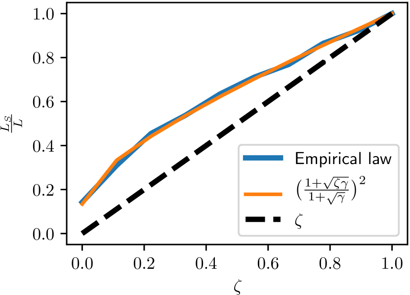
This is a direct application of the Marchenko-Pastur law (Marchenko and Pastur, 1967). The law is illustrated on a toy dataset in Figure D.1. In Proposition 3.4, $\gamma$ is the ratio between the number of atoms and number of dimensions, and the average size of $S$ is described by $\zeta\leq 1~{}.$ In an overcomplete setting, we have $\gamma\gg 1~{},$ yielding the approximation of Equation 9: $L_{S}\simeq\zeta L~{}.$ Therefore, if $z^{*}$ is very sparse ($\zeta\ll 1$), the convergence rates of Proposition 3.2 are much better than those of ISTA.

Example

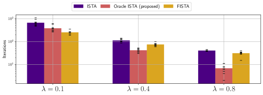
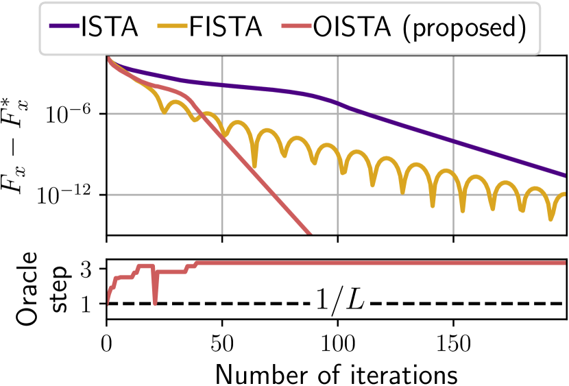
Figure 2 compares the OISTA, ISTA, and FISTA on a toy problem. The improved rate of convergence of OISTA is illustrated. Further comparisons are displayed in Figure D.2 for different regularization parameters $\lambda~{}.$ While this demonstrates a much faster rate of convergence, it requires computing several Lipschitz constants $L_{S}~{},$ which is cumbersome in high dimension. This motivates the next section, where we propose to learn those steps.

Figure 2: Convergence curves of OISTA, ISTA, and FISTA on a toy problem with $n=10~{},$ $m=50~{},$ $\lambda=0.5~{}.$ The bottom figure displays the (normalized) steps taken by OISTA at each iteration. Full experimental setup described in Appendix D.

4 Learning unfolded algorithms

Network architectures

At each step, ISTA performs a linear operation to compute an update in the direction of the gradient $D^{\top}(Dz^{(t)}-x)$ and then an element-wise non linearity with the soft-thresholding operator $\operatorname{ST}.$ The whole algorithm can be summarized as a recurrent neural network (RNN), presented in 3(a). Gregor and Le Cun (2010) introduced Learned-ISTA (LISTA), a neural network constructed by unfolding this RNN $T$ times and learning the weights associated to each layer. The unfolded network, presented in 3(b), iterates $z^{(t+1)}=\operatorname{ST}(W_{x}^{(t)}x+W_{z}^{(t)}z^{(t)},\lambda\beta^{(t)})~{}.$ It outputs exactly the same vector as $T$ iterations of ISTA when $W_{x}^{(t)}=\frac{D^{\top}}{L}~{},$ $W_{z}^{(t)}=\operatorname{Id}_{m}-\frac{D^{\top}D}{L}$ and $\beta^{(t)}=\frac{1}{L}~{}.$ Empirically, this network is able to output a better estimate of the sparse code solution with fewer operations.

(a) ISTA - Recurrent Neural Network

(b) LISTA - Unfolded network with $T=3$

Figure 3: Network architecture for ISTA (left) and LISTA (right).

Due to the expression of the gradient, Chen et al. (2018) proposed to consider only a subclass of the previous networks, where the weights $W_{x}$ and $W_{z}$ are coupled via $W_{z}=\operatorname{Id}_{m}-W_{x}^{\top}D~{}.$ This is the architecture we consider in the following. A layer of LISTA is a function $\phi_{\theta}:\mathbb{R}^{m}\times\mathbb{R}^{n}\to\mathbb{R}^{m}$ parametrized by $\theta=(W,\alpha,\beta)\in\mathbb{R}^{n\times m}\times\mathbb{R}^{+}_{*}\times\mathbb{R}^{+}_{*}$ such that

$$\phi_{\theta}(z,x)=\operatorname{ST}(z-\alpha W^{\top}(Dz-x),\beta\lambda)\enspace.$$ (10)

Given a set of $T$ layer parameters $\Theta^{(T)}=\{\theta^{(t)}\}_{t=0}^{T-1}~{},$ the LISTA network $\Phi_{\Theta^{(T)}}:\mathbb{R}^{n}\to\mathbb{R}^{m}$ is $\Phi_{\Theta^{(T)}}(x)=z^{(T)}(x)$ where $z^{(t)}(x)$ is defined by recursion

$$z^{(0)}(x)=0,~{}~{}\text{and }~{}~{}~{}z^{(t+1)}(x)=\phi_{\theta^{(t)}}(z^{(t)}(x),x)~{}~{}\text{ for }~{}t\in\llbracket 0,T-1\rrbracket\enspace.$$ (11)

Taking $W=D~{},$ $\alpha=\beta=\frac{1}{L}$ yields the same outputs as $T$ iterations of ISTA.

To alleviate the need to learn the large matrices $W^{(t)},$ Liu et al. (2019) proposed to use a shared analytic matrix $W_{\text{ALISTA}}$ for all layers. The matrix is computed in a preprocessing stage by

$$W_{\text{ALISTA}}=\operatorname*{arg\,min}_{W}\|W^{\top}D\|_{F}^{2}~{}~{}~{}~{}s.t.~{}~{}~{}~{}\text{diag}(W^{\top}D)={\boldsymbol{1}}_{m}\enspace.$$ (12)

Then, only the parameters $(\alpha^{(t)},\beta^{(t)})$ are learned. This effectively reduces the number of parameters from $(nm+2)\times T$ to $2\times T~{}.$ However, we will see that ALISTA fails in our setup.

Step-LISTA

With regards to the study on step sizes for ISTA in Section 3, we propose to learn approximation of ISTA step sizes for the input distribution using the LISTA framework. The resulting network, dubbed Step-LISTA (SLISTA), has $T$ parameters $\Theta_{\text{SLISTA}}=\{\alpha^{(t)}\}_{t=0}^{T-1}~{},$ and follows the iterations:

$$z^{(t+1)}(x)=\operatorname{ST}(z^{(t)}(x)-\alpha^{(t)}D^{\top}(Dz^{(t)}(x)-x),\alpha^{(t)}\lambda)\enspace.$$ (13)

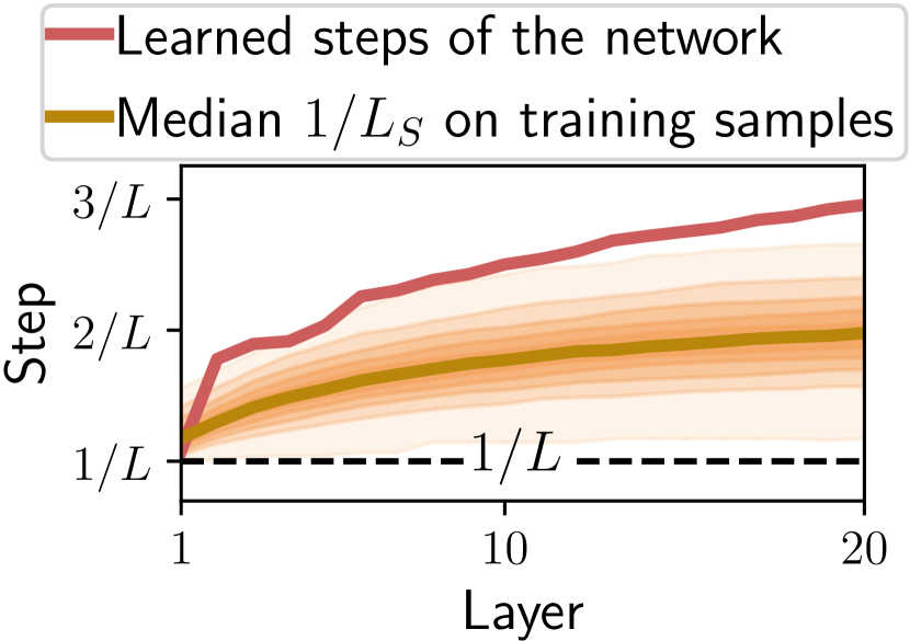
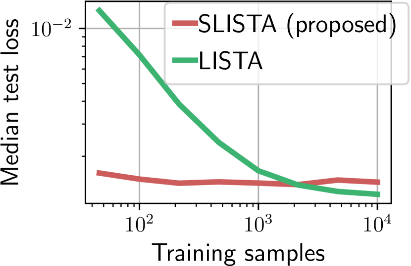
This is equivalent to a coupling in the LISTA parameters: a LISTA layer $\theta=(W,\alpha,\beta)$ corresponds to a SLISTA layer if and only if $\frac{\alpha}{\beta}W=D$. This network aims at learning good step sizes, like the ones used in OISTA, without the computational burden of computing Lipschitz constants. The number of parameters compared to the classical LISTA architecture $\Theta_{\text{LISTA}}$ is greatly diminished, making the network easier to train. Learning curves are shown in Figure D.3 in appendix. Figure 4 displays the learned steps of a SLISTA network on a toy example. The network learns larger step-sizes as the $1/L_{S}$’s increase.

Figure 4: Steps learned with a $20$ layers SLISTA network on a $10\times 20$ problem. For each layer $t$ and each training sample $x$, we compute the support $S(x,t)$ of $z^{(t)}(x)$. The brown curves display the quantiles of the distribution of $1/L_{S(x,t)}$ for each layer $t~{}$. Full experimental setup described in Appendix D.

Training the network

We consider the framework where the network learns to solve the Lasso on $\mathcal{B}_{\infty}$ in an unsupervised way. Given a distribution $p$ on $\mathcal{B}_{\infty}~{},$ the network is trained by solving

$$\tilde{\Theta}^{(T)}\in\arg\min_{\Theta^{(T)}}\mathcal{L}(\Theta^{(T)})\triangleq\mathbb{E}_{x\sim p}[F_{x}(\Phi_{\Theta^{(T)}}(x))]\enspace.$$ (14)

Most of the literature on learned optimization train the network with a different supervised objective (Gregor and Le Cun, 2010; Xin et al., 2016; Chen et al., 2018; Liu et al., 2019). Given a set of pairs $(x^{i},z^{i})~{},$ the supervised approach tries to learn the parameters of the network such that $\Phi_{\Theta}(x^{i})\simeq z^{i}$ e.g.  by minimizing $\|\Phi_{\Theta}(x^{i})-z^{i}\|^{2}~{}.$ This training procedure differs critically from ours. For instance, ISTA does not converge for the supervised problem in general while it does for the unsupervised one. As Proposition 4.1 shows, the unsupervised approach allows to learn to minimize the Lasso cost function $F_{x}~{}.$

Proposition 4.1 (Pointwise convergence).

Let $\tilde{\Theta}^{(T)}$ found by solving Problem (14).
For $x\in\mathcal{B}_{\infty}$ such that $p(x)>0~{},$ $F_{x}(\Phi_{\tilde{\Theta}^{(T)}}(x))\xrightarrow[T\to+\infty]{}F_{x}^{*}$ almost everywhere.

Proof.

Let $\Theta_{\text{ISTA}}^{(T)}$ the parameters corresponding to ISTA i.e.  $\theta_{\text{ISTA}}^{(t)}=(D,1/L,1/L)~{}.$ For all $T~{},$ we have $\mathbb{E}_{x\sim p}[F_{x}^{*}]\leq\mathbb{E}_{x\sim p}[F_{x}(\Phi_{\tilde{\Theta}^{(T)}}(x))]\leq\mathbb{E}_{x\sim p}[F_{x}(\Phi_{\Theta_{\text{ISTA}}^{(T)}}(x))]~{}.$ Since ISTA converges uniformly on any compact, the right hand term goes to $\mathbb{E}_{x\sim p}[F_{x}^{*}]~{}.$ Therefore, by the squeeze theorem, $\mathbb{E}_{x\sim p}[F_{x}(\Phi_{\tilde{\Theta}^{(T)}}(x))-F_{x}^{*}]\to 0~{}.$ This implies almost sure convergence of $F_{x}(\Phi_{\tilde{\Theta}^{(T)}}(x))-F_{x}^{*}$ to $0$ since it is non-negative. ∎

Asymptotical weight coupling theorem

In this paragraph, we show the main result of this paper: any LISTA network minimizing $F_{x}$ on $\mathcal{B}_{\infty}$ reduces to SLISTA in its deep layers (Theorem 4.4). It relies on the following Lemmas.

Lemma 4.2 (Stability of solutions around $D_{j}$).

Let $D\in\mathbb{R}^{n\times m}$ be a dictionary with non-duplicated unit-normed columns. Let $c\triangleq\max_{l\neq j}|D_{l}^{\top}D_{j}|<1~{}.$ Then for all $j\in\llbracket 1,m\rrbracket$ and $\varepsilon\in\mathbb{R}^{m}$ such that $\|\varepsilon\|<\lambda(1-c)$ and $D_{j}^{\top}\varepsilon=0~{},$ the vector $(1-\lambda)e_{j}$ minimizes $F_{x}$ for $x=D_{j}+\varepsilon~{}.$

It can be proven by verifying the KKT conditions (3) for $(1-\lambda)e_{j}~{},$ detailed in Subsection C.1.

Lemma 4.3 (Weight coupling).

Let $D\in\mathbb{R}^{n\times m}$ be a dictionary with non-duplicated unit-normed columns. Let $\theta=(W,\alpha,\beta)$ a set of parameters. Assume that all the couples $(z^{*}(x),x)\in\mathbb{R}^{m}\times\mathcal{B}_{\infty}$ such that $z^{*}(x)\in\operatorname*{arg\,min}F_{x}(z)$ verify $\phi_{\theta}(z^{*}(x),x)=z^{*}(x)$. Then, $\frac{\alpha}{\beta}W=D~{}.$

Sketch of proof (full proof in Subsection C.2).

For $j\in\llbracket 1,m\rrbracket~{},$ consider $x=D_{j}+\varepsilon~{},$ with $\varepsilon^{\top}D_{j}=0~{}.$ For $\|\varepsilon\|$ small enough, $x\in\mathcal{B}_{\infty}$ and $\varepsilon$ verifies the hypothesis of 4.2, therefore $z^{*}=(1-\lambda)e_{j}\in\operatorname*{arg\,min}F_{x}~{}.$ Writing $\phi_{\theta}(z^{*},x)=z^{*}$ for the $j$-th coordinate yields $\alpha W_{j}^{\top}(\lambda D_{j}+\varepsilon)=\lambda\beta~{}.$ We can then verify that $(\alpha W_{j}^{\top}-\beta D_{j}^{\top})(\lambda D_{j}+\varepsilon)=0~{}.$ This stands for any $\varepsilon$ orthogonal to $D_{j}$ and of norm small enough. Simple linear algebra shows that this implies $\alpha W_{j}-\beta D_{j}=0~{}.$ ∎

4.3 states that the Lasso solutions are fixed points of a LISTA layer only if this layer corresponds to a step size for ISTA. The following theorem extends the lemma by continuity, and shows that the deep layers of any converging LISTA network must tend toward a SLISTA layer.

Theorem 4.4.

Let $D\in\mathbb{R}^{n\times m}$ be a dictionary with non-duplicated unit-normed columns. Let $\Theta^{(T)}=\{\theta^{(t)}\}_{t=0}^{T}$ be the parameters of a sequence of LISTA networks such that the transfer function of the layer $t$ is $z^{(t+1)}=\phi_{\theta^{(t)}}(z^{(t)},x)~{}.$ Assume that

1. the sequence of parameters converges i.e.  $\theta^{(t)}\xrightarrow[t\to\infty]{}\theta^{*}=(W^{*},\alpha^{*},\beta^{*})\enspace,$

2. the output of the network converges toward a solution $z^{*}(x)$ of the Lasso (1) uniformly over the equiregularization set $\mathcal{B}_{\infty}~{},$ i.e.  $\sup_{x\in\mathcal{B}_{\infty}}\|\Phi_{\Theta^{(T)}}(x)-z^{*}(x)\|\xrightarrow[T\to\infty]{}0$  .

Then $\frac{\alpha^{*}}{\beta^{*}}W^{*}=D\enspace.$

Sketch of proof (full proof in Subsection C.3).

Let $\varepsilon>0~{},$ and $x\in\mathcal{B}_{\infty}~{}.$ Using the triangular inequality, we have

$$\|\phi_{\theta^{*}}(z^{*},x)-z^{*}\| \leq \|\phi_{\theta^{*}}(z^{*},x)-\phi_{\theta^{(t)}}(z^{(t)},x)\|+\|\phi_{\theta^{(t)}}(z^{(t)},x)-z^{*}\|$$ (15)

Since the $z^{(t)}$ and $\theta^{(t)}$ converge, they are valued over a compact set $K$. The function $f:(z,x,\theta)\mapsto\phi_{\theta}(z,x)$ is continuous, piecewise-linear. It is therefore Lipschitz on $K$. Hence, we have $\|\phi_{\theta^{*}}(z^{*},x)-\phi_{\theta^{(t)}}(z^{(t)},x)\|\leq\varepsilon$ for $t$ large enough. Since $\phi_{\theta^{(t)}}(z^{(t)},x)=z^{(t+1)}$ and $z^{(t)}\to z^{*}~{},$ $\|\phi_{\theta^{(t)}}(z^{(t)},x)-z^{*}\|\leq\varepsilon$ for $t$ large enough. Finally, $\phi_{\theta^{*}}(z^{*},x)=z^{*}~{}.$ 4.3 allows to conclude. ∎

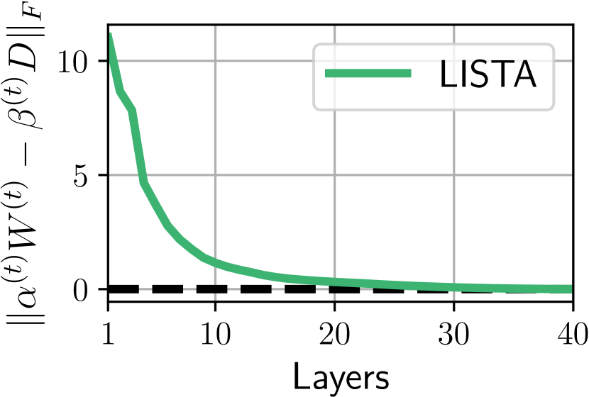
Figure 5: Illustration of Theorem 4.4: for deep layers of LISTA, we have $\|\alpha^{(t)}W^{(t)}-\beta^{(t)}D\|_{F}\to 0~{},$ indicating that the network ultimately only learns a step size. Full experimental setup described in Appendix D.

Theorem 4.4 means that the deep layers of any LISTA network that converges to solutions of the Lasso correspond to SLISTA iterations: $W^{(t)}$ aligns with $D~{},$ and $\alpha^{(t)},\beta^{(t)}$ get coupled. This is illustrated in Figure 5, where a 40-layers LISTA network is trained on a $10\times 20$ problem with $\lambda=0.1~{}.$ As predicted by the theorem, $\frac{\alpha^{(t)}}{\beta^{(t)}}W^{(t)}\to D~{}.$ The last layers only learn a step size. This is consistent with the observation of Moreau and Bruna (2017) which shows that the deep layers of LISTA stay close to ISTA. Further, Theorem 4.4 also shows that it is hopeless to optimize the unsupervised objective (14) with $W_{\text{ALISTA}}$ (12), since this matrix is not aligned with $D~{}.$

5 Numerical Experiments

This section provides numerical arguments to compare SLISTA to LISTA and ISTA. All the experiments were run using Python (Python Software Foundation, 2017) and pytorch (Paszke et al., 2017). The code to reproduce the figures is available online.

Network comparisons

We compare the proposed approach SLISTA to state-of-the-art learned methods LISTA (Chen et al., 2018) and ALISTA (Liu et al., 2019) on synthetic and semi-real cases.

In the synthetic case, a dictionary $D\in\mathbb{R}^{n\times m}$ of Gaussian i.i.d. entries is generated. Each column is then normalized to one. A set of Gaussian i.i.d. samples $(\tilde{x}^{i})_{i=1}^{N}\in\mathbb{R}^{n}$ is drawn. The input samples are obtained as $x^{i}=\tilde{x}^{i}/\|D^{\top}\tilde{x}^{i}\|_{\infty}~\in\mathcal{B}_{\infty}~{},$ so that for all $i~{},$ $x^{i}\in\mathcal{B}_{\infty}~{}.$ We set $m=256$ and $n=64$.

For the semi-real case, we used the digits dataset from scikit-learn (Pedregosa et al., 2011) which consists of $8\times 8$ images of handwritten digits from $0$ to $9~{}.$ We sample $m=256$ samples at random from this dataset and normalize it do generate our dictionary $D~{}.$ Compared to the simulated Gaussian dictionary, this dictionary has a much richer correlation structure, which is known to imper the performances of learned algorithms (Moreau and Bruna, 2017). The input distribution is generated as in the simulated case.

The networks are trained by minimizing the empirical loss $\mathcal{L}$ (14) on a training set of size $N_{\text{train}}=10,000$ and we report the loss on a test set of size $N_{\text{test}}=10,000~{}.$ Further details on training are in Appendix D.

Figure 6: Test loss of ISTA, ALISTA, LISTA and SLISTA on simulated and semi-real data for different regularization parameters.

Figure 6 shows the test curves for different levels of regularization $\lambda=0.1$ and $0.8$. SLISTA performs best for high $\lambda$, even for challenging semi-real dictionary $D~{}.$ In a low regularization setting, LISTA performs best as SLISTA cannot learn larger steps due to the low sparsity of the solution. In this unsupervised setting, ALISTA does not converge in accordance with Theorem 4.4.

6 Conclusion

We showed that using larger step sizes is an efficient strategy to accelerate ISTA for sparse solution of the Lasso. In order to make this approach practical, we proposed SLISTA, a neural network architecture which learns such step sizes. Theorem 4.4 shows that the deepest layers of any converging LISTA architecture must converge to a SLISTA layer. Numerical experiments show that SLISTA outperforms LISTA in a high sparsity setting. An major benefit of our approach is that it preserves the dictionary. We plan on leveraging this property to apply SLISTA in convolutional or wavelet cases, where the structure of the dictionary allows for fast multiplications.

Appendix A Unfolded optimization algorithms literature summary

In Table A.1, we summarize the prolific literature on learned unfolded optimization procedures for sparse recovery. A particular focus is set on the chosen training loss training which is either supervised, with a regression of $z^{i}$ from the input $x^{i}$ for a given training set $(x^{i},z^{i})$, or unsupervised, where the objective is to minimize the Lasso cost function $F_{x}$ for each training point $x$.

Table A.1: Neural network for sparse coding

Reference	Base Algo	Train Loss	Coupled weights	Remarks
Gregor and Le Cun (2010)	ISTA / CD	supervised	$\times$	–
Sprechmann et al. (2012)	Block CD	unsupervised	$\times$	Group $\ell_{1}$
Sprechmann et al. (2013)	ADMM	supervised	N/A	–
Hershey et al. (2014)	NMF	supervised	$\times$	NMF
Wang et al. (2015)	IHT	supervised	$\times$	Hard-thresholding
Xin et al. (2016)	IHT	supervised	$\times$/$\checkmark$	Hard-thresholding
Giryes et al. (2018)	PGD/IHT	supervised	N/A	Group $\ell_{1}$
Yang et al. (2017)	ADMM	supervised	N/A	–
Adler et al. (2017)	ADMM	supervised	N/A	Wasserstein distance with $z^{*}$
Borgerding et al. (2017)	AMP	supervised	$\times$	–
Moreau and Bruna (2017)	ISTA	unsupervised	$\times$	–
Chen et al. (2018)	ISTA	supervised	$\checkmark$	Linear convergence rate
Ito et al. (2018)	ISTA	supervised	$\checkmark$	MMSE shrinkage non-linearity
Zhang and Ghanem (2018)	PGD	supervised	$\checkmark$	Sparsity of Wavelet coefficients
Liu et al. (2019)	ISTA	supervised	$\checkmark$	Analytic weight $W_{\text{ALISTA}}$
Proposed	ISTA	unsupervised	$\checkmark$	–

Appendix B Proofs of Section 3’s results

B.1 Proof of Proposition 3.1

We consider that the solution of the Lasso is unique, following the result of Tibshirani (2013)[Lemmas 4 and 16] when the entries of $D$ and $x$ come from a continuous distribution.

See 3.1

Proof.

Let $z^{(t)}$ be the sequence of iterates produced by Algorithm 1. We have a descent function

$$F_{x}(z^{(t+1)})-F_{x}(z^{(t)})\leq-\frac{\gamma}{2}\|z^{(t+1)}-z^{(t)}\|^{2}\leq-\frac{\min\|D_{j}\|}{2}\|z^{(t+1)}-z^{(t)}\|^{2}\enspace,$$ (16)

where $\gamma=L_{S}$ if Section 3 is met, and $L$ otherwise. Additionally, the iterates are bounded because $F_{x}(z^{(t)})$ decreases at each iteration and $F_{x}$ is coercive. Hence we can apply Zangwill’s Global Convergence Theorem (Zangwill, 1969). Any $z^{*}$ accumulation point of $(z^{(t)})_{t\in\mathbb{N}}$ is a minimizer of $F_{x}~{}.$

Since we only consider the case where the minimizer is unique, the bounded sequence $(z^{(t)})_{t\in\mathbb{N}}$ has a unique accumulation point, thus converges to $z^{*}~{}.$

The support identification is a simplification of a result of Hale et al. (2008), we include it here for completeness.

Lemma B.1 (Approximation of the soft-thresholding).

Let $z\in\mathbb{R},\nu>0~{}.$ For $\epsilon$ small enough, we have

$$\operatorname{ST}(z+\epsilon,\nu)=\begin{cases}\begin{aligned} &0\enspace,&\mathrm{\quad if\,}|z|<\nu\enspace,\\ &\max(0,\epsilon)\operatorname*{sign}(z)\enspace,&\mathrm{\quad if\,}|z|=\nu\enspace,\\ &z+\epsilon-\nu\operatorname*{sign}{z}\enspace,&\mathrm{\quad if\,}|z|>\nu\enspace.\end{aligned}\end{cases}$$ (17)

Let $\rho>0$ be such that Equation 17 holds for $\nu=\lambda/L~{},$ every $\epsilon<\rho~{},$ and every $z=z_{j}^{*}-\frac{1}{L}D_{j}^{\top}(Dz^{*}-x)~{}.$

Let $t\in\mathbb{N}$ such that $z^{(t)}=z^{*}+\epsilon~{},$ with $\|\epsilon\|\leq\rho~{}.$ With $\epsilon^{\prime}\triangleq(\operatorname{Id}-\frac{1}{L}D^{\top}D)\epsilon~{},$ we also have $\|\epsilon^{\prime}\|\leq\rho~{}.$ Let $j\in\llbracket 1,m\rrbracket~{}.$

If $j\notin E~{},$ $|z_{j}^{*}-\frac{1}{L}D_{j}^{\top}(Dz^{*}-x)|=|\frac{1}{L}D_{j}^{\top}(Dz^{*}-x)|<\lambda/L$ hence $\operatorname{ST}(z_{j}^{*}-\frac{1}{L}D_{j}^{\top}(Dz^{*}-x)+\epsilon^{\prime}_{j},\lambda/L)=0~{}.$

If $j\in E~{},$ $|z_{j}^{*}-\frac{1}{L}D_{j}^{\top}(Dz^{*}-x)|=|z^{*}_{j}+\frac{\lambda}{L}\operatorname*{sign}z^{*}_{j}|>\lambda/L~{},$ and $\operatorname*{sign}\operatorname{ST}(z_{j}^{*}-\frac{1}{L}D_{j}^{\top}(Dz^{*}-x)+\epsilon^{\prime}_{j},\lambda/L)=\operatorname*{sign}z^{*}_{j}~{}.$

The same reasoning can be applied with $\rho^{\prime}$ such that Equation 17 holds for $\nu=\lambda/L_{S^{*}}~{},$ every $\epsilon<\rho^{\prime}~{},$ and every $z=z_{j}^{*}-\frac{1}{L_{S}^{*}}D_{j}^{\top}(Dz^{*}-x)$. If we introduce $\eta>0$ such that $\|\epsilon\|\leq\eta\implies\|(\operatorname{Id}-\frac{1}{L_{S^{*}}}D\top D)\epsilon\|\leq\rho^{\prime}~{},$ in the ball of center $z^{*}$ and radius $\eta~{},$ the iteration with step size $L_{S^{*}}$ identifies the support.

Additionnally, since $\operatorname{Id}-\frac{1}{L_{S^{*}}}D_{S^{*}}^{\top}D_{S^{*}}$ is non expansive on vectors which support is $S^{*}~{},$ the iterations with the step $L_{S^{*}}$ never leave this ball once they have entered it.

Therefore, once the iterates enter $\mathcal{B}(z^{*},\min(\eta,\rho))~{},$ Section 3 is always satisfied.

∎

B.2 Proof of Proposition 3.2

See 3.2

Proof.

For $t\geq T^{*}~{},$ the iterates support is $S^{*}$ and the objective function is $L_{S^{*}}$-smooth instead of $L$-smooth. It is also $\mu^{*}$ strongly convex if $\mu^{*}>0~{}.$ The obtained rates are a classical result of the proximal gradient descent method in these cases. ∎

Appendix C Proof of Section 4’s Lemmas

C.1 Proof of 4.2

See 4.2

Proof.

Let $j\in\llbracket 1,m\rrbracket$ and let $\varepsilon\in\mathbb{R}^{m}\cap D_{j}^{\perp}$ be a vector such that $\|\varepsilon\|<\lambda(1-c)~{}.$
For notation simplicity, we denote $z^{*}=z^{*}(D_{j}-\varepsilon)~{}.$

$$D^{\top}_{j}(Dz^{*}-D_{j}-\varepsilon) =D^{\top}_{j}(-\lambda D_{j}-\varepsilon)=-\lambda=-\lambda\operatorname*{sign}z^{*}_{j}~{},$$ (18)

since $1-\lambda>0~{}.$ For the other coefficients $l\in\llbracket 1,m\rrbracket\setminus\{j\}~{},$ we have

$$|D^{\top}_{l}(Dz^{*}-D_{j}-\varepsilon)| =|D^{\top}_{l}(-\lambda D_{j}-\varepsilon)|~{},$$ (19)

$$=|\lambda D^{\top}_{l}D_{j}+D^{\top}_{l}\varepsilon)|~{},$$ (20)

$$\leq\lambda|D^{\top}_{l}D_{j}|+|D_{l}^{\top}\varepsilon|~{},$$ (21)

$$\leq\lambda c+\|D_{l}\|\|\varepsilon\|~{},$$ (22)

$$\leq\lambda c+\|\varepsilon\|<\lambda~{},$$ (23)

Therefore, $(1-\lambda)e_{j}$ verifies the KKT conditions (3) and $z^{*}(D_{j}+\varepsilon)=(1-\lambda)e_{j}~{}.$ ∎

C.2 Proof of 4.3

See 4.3

Proof.

Let $x\in\mathcal{B}_{\infty}$ be an input vector and $z^{*}(x)\in\mathbb{R}^{m}$ be a solution for the Lasso at level $\lambda>0~{}.$ Let $j\in\llbracket 1,m\rrbracket$ be such that $z^{*}_{j}>0~{}.$ The KKT conditions (3) gives

$$D_{j}^{\top}(Dz^{*}(x)-x)=-\lambda\enspace.$$ (25)

Suppose that $z^{*}(x)$ is a fixed point of the layer, then we have

$$\operatorname{ST}(z^{*}_{j}(x)-\alpha W_{j}^{\top}(Dz^{*}(x)-x),\lambda\beta)=z_{j}^{*}(x)>0\enspace.$$ (26)

By definition, $\operatorname{ST}(a,b)>0$ implies that $a>b$ and $\operatorname{ST}(a,b)=a-b~{}.$ Thus,

$$z^{*}_{j}(x)-\alpha W_{j}^{\top}(Dz^{*}(x)-x)-\lambda\beta=z_{j}^{*}(x)$$ (27)

$$\Leftrightarrow~{}~{}~{}~{}~{} \alpha W_{j}^{\top}(Dz^{*}(x)-x)+\lambda\beta=0$$ (28)

$$\Leftrightarrow~{}~{}~{}~{}~{} \alpha W_{j}^{\top}(Dz^{*}(x)-x)-\beta D_{j}^{\top}(Dz^{*}(x)-x)=0\quad\quad\text{by \eqref{eq:weigh_coupling:kkt}}$$ (29)

$$\Leftrightarrow~{}~{}~{}~{}~{} (\alpha W_{j}-\beta D_{j})^{\top}(Dz^{*}(x)-x)=0\enspace.$$ (30)

As the relation (30) must hold for all $x\in\mathcal{B}_{\infty}~{},$ it is true for all $D_{j}+\varepsilon$ for all $\varepsilon\in\mathcal{B}(0,\lambda(1-c))\cap D_{j}^{\perp}~{}.$ Indeed, in this case, $\|D^{\top}(D_{j}+\varepsilon)\|_{\infty}=1~{}.$ $D$ verifies the conditions of Lemma 4.2, and thus $z^{*}=(1-\lambda)e_{j}~{},$ i.e.

$$(\alpha W_{j}-\beta D_{j})^{\top}(D(1-\lambda)e_{j}-(D_{j}+\varepsilon)) =0$$ (31)

$$(\alpha W_{j}-\beta D_{j})^{\top}\left(-\lambda D_{j}-\varepsilon\right) =0$$ (32)

Taking $\varepsilon=0$ yields $(\alpha W_{j}-\beta D_{j})^{\top}D_{j}=0~{},$ and therefore Eq. (32) becomes $(\alpha W_{j}-\beta D_{j})^{\top}\varepsilon=0$ for all $\varepsilon$ small enough and orthogonal to $D_{j}~{},$ which implies $\alpha W_{j}-\beta D_{j}=0$ and concludes our proof. ∎

C.3 Proof of Theorem 4.4

See 4.4

Proof.

For simplicity of the notation, we will drop the $x$ variable whenever possible, i.e.  $z^{*}=z^{*}(x)$ and $\phi_{\theta}(z)=\phi_{\theta}(z,x)~{}.$ We denote $z^{(t)}=\Phi_{\Theta^{(t)}}(x)$ the output of the network with $t$ layers.
Let $\epsilon>0~{}.$ By hypothesis (i), there exists $T_{0}$ such that for all $t\geq T_{0}~{},$

$$\|W^{(t)}-W^{*}\|\leq\epsilon~{}~{}~{}|\alpha^{(t)}-\alpha^{*}|\leq\epsilon~{}~{}~{}|\beta^{(t)}-\beta^{*}|\leq\epsilon~{}.$$ (33)

By hypothesis (ii), , there exists $T_{1}$ such that for all $t\geq T_{1}$ and all $x\in\mathcal{B}_{\infty}~{},$

$$\|z^{(t)}-z^{*}\|\leq\epsilon~{}.$$ (34)

Let $x\in\mathcal{B}_{\infty}$ be an input vector and $t\geq\max(T_{0},T_{1})~{}.$ Using (34), we have

$$\|z^{(t+1)}-z^{(t)}\| \leq \|z^{(t+1)}-z^{*}\|+\|z^{(t)}-z^{*}\|\leq 2\epsilon$$ (35)

By (i), there exist a compact set $\mathcal{K}_{1}\subset\mathbb{R}^{n\times m}\times\mathbb{R}^{+}_{*}\times\mathbb{R}^{+}_{*}$ s.t. $\theta^{(t)}\in\mathcal{K}_{1}$ for all $t\in\mathbb{N}$ and $\theta^{*}\in\mathcal{K}~{}.$ The input $x$ is taken in a compact set $\mathcal{B}_{\infty}$ and as $z^{*}=\operatorname*{arg\,min}_{z}F_{x}(z)~{},$ we have $\lambda\|z\|_{1}\leq F_{x}(z^{*})\leq F_{x}(0)=\|x\|$ thus $z^{*}$ is also in a compact set $\mathcal{K}_{2}~{}.$
We consider the function $f(z,x,\theta)=\operatorname{ST}(z-\alpha W^{\top}(Dz-x),\beta)$ on the compact set $\mathcal{K}_{2}\times\mathcal{B}_{\infty}\times\mathcal{K}_{1}~{}.$ This function is continuous and piece-wise linear on a compact set. It is thus $L$-Lipschitz and thus

$$\|\phi_{\theta^{(t)}}(z^{(t)})-\phi_{\theta^{(t)}}(z^{*})\| \leq L\|z^{(t)}-z^{*}\|\leq L\epsilon$$ (36)

$$\|\phi_{\theta^{*}}(z^{*})-\phi_{\theta^{(t)}}(z^{*})\| \leq L\|\theta^{(t)}-\theta^{*}\|\leq L\epsilon$$ (37)

Using these inequalities, we get

$$\|\phi_{\theta^{*}}(z^{*},x)-z^{*}\| \leq \underbrace{\|\phi_{\theta^{*}}(z^{*})-\phi_{\theta^{(t)}}(z^{*})\|}_{<L\epsilon~{}\text{by \eqref{eq:thm:fhs}}}+\underbrace{\|\phi_{\theta^{(t)}}(z^{*})-\phi_{\theta^{(t)}}(z^{(t)})\|}_{<L\epsilon~{}\text{by \eqref{eq:thm:shs}}}$$

$$+\underbrace{\|\phi_{\theta^{(t)}}(z^{(t)})-z^{(t)}\|}_{<2\epsilon~{}\text{ by \eqref{eq:thm:cauchy_cvg}}}+\underbrace{\|z^{(t)}-z^{*}\|}_{<\epsilon~{}\text{ by \eqref{eq:thm:iterate_cvg}}}$$

$$\leq (2L+3)\epsilon~{}.$$ (39)

As this result holds for all $\epsilon>0$ and all $x\in\mathcal{B}_{\infty}~{},$ we have $\phi_{\theta^{*}}(z^{*})=z^{*}$ for all $x\in\mathcal{B}_{\infty}~{}.$ We can apply the 4.3 to conclude this proof. ∎

Appendix D Experimental setups and supplementary figures

Dictionary generation: Unless specified otherwise, to generate synthetic dictionaries, we first draw a random i.i.d. Gaussian matrix $\hat{D}\in\mathbb{R}^{n\times m}$. The dictionary is obtained by normalizing the columns: $D_{ij}=\frac{1}{\|\hat{D}_{i:}\|}\hat{D}_{ij}$.

Samples generation: The samples $x$ are generated as follows: Random i.i.d. Gaussian samples $\hat{x}\in~\mathbb{R}^{n}$ are generated. We then normalize them: $x=\frac{1}{\|D^{\top}\hat{x}\|_{\infty}}\hat{x}$, so that $x\in\mathcal{B}_{\infty}$.

Training the networks Since the loss function and the network are continuous but non-differentiable, we use sub-gradient descent for training. The sub-gradient of the cost function with respect to the parameters of the network is computed by automatic differentiation. We use full-batch sub-gradient descent with a backtracking procedure to find a suitable learning rate. To verify that we do not overfit the training set, we always check that the test loss and train loss are comparable.

Main text figures setup

• Figure 2: We generate a random dictionary of size $10\times 50$. We take $\lambda=0.5$, and a random sample $x\in\mathcal{B}_{\infty}$. $F_{x}^{*}$ is computed by iterating ISTA for $10000$ iterations.

• Figure 4: We generate a random dictionary of size $10\times 20$. We take $\lambda=0.2$. We generate a training set of $N=1000$ samples $(x^{i})_{i=1}^{1000}\in\mathcal{B}_{\infty}$. A 20 layers SLISTA network is trained by gradient descent on these data. We report the learned step sizes. For each layer $t$ of the network and each training sample $x$, we compute the support at the output of the $t$-th layer, $S(x,t)=\operatorname*{supp}(z^{(t)}(x))$. For each $t$, we display the quantiles of the distribution of the $(1/L_{S(x^{i},t)})_{i=1}^{1000}$.

• Figure 5: A random $10\times 20$ dictionary is generated. We take $1000$ training samples, and $\lambda=0.05$. A $40$ layers LISTA network is trained by gradient descent on those samples. We report the quantity $\|\alpha^{(t)}W^{(t)}-\beta^{(t)}D\|_{F}$ for each layer $t$.

Supplementary experiments

.

Figure D.1: Illustration of Proposition 3.4. A toy Gaussian dictionary is generated with $n=200~{},$ $m=600$ so that $\gamma=3~{}.$ We compute its Lipschitz constant $L~{}.$ For $\zeta$ between $0$ and $1~{},$ we extract $\lfloor\zeta m\rfloor$ columns at random and compute the corresponding Lipschitz constant $L_{S}~{}.$ The plot shows an almost perfect fit between the empirical law and the theoretical limit (9).

Figure D.2: Comparison between ISTA, FISTA and Oracle-ISTA for different levels of regularization on a Gaussian dictionnary, with $n=100$ and $m=200$. We report the average number of iterations taken to reach a point $z$ such that $F_{x}(z)<F^{*}_{x}+10^{-13}$. The experiment is repeated $10$ times, starting from random points in $\mathcal{B}_{\infty}$. OISTA is always faster than ISTA, and is faster than FISTA for high regularization.

Figure D.3: Learning curves of SLISTA and LISTA. Random Gaussian dictionaries with $n=10$ and $m=20$ are generated. We take $\lambda=0.3$. Networks with 10 layers are fit on those dictionaries, and their test loss is reported for different number of training samples. The process is repeated $100$ times; the curves shown display the median of the test-loss.

References

• Adler et al. (2017) Jonas Adler, Axel Ringh, Ozan Öktem, and Johan Karlsson. Learning to solve inverse problems using Wasserstein loss. preprint ArXiv, 1710.10898, 2017.
• Beck and Teboulle (2009) Amir Beck and Marc Teboulle. A fast iterative shrinkage-thresholding algorithm for linear inverse problems. SIAM journal on imaging sciences, 2(1):183–202, 2009.
• Borgerding et al. (2017) Mark Borgerding, Philip Schniter, and Sundeep Rangan. AMP-inspired deep networks for sparse linear inverse problems. IEEE Transactions on Signal Processing, 65(16):4293–4308, 2017.
• Chen et al. (2018) Xiaohan Chen, Jialin Liu, Zhangyang Wang, and Wotao Yin. Theoretical linear convergence of unfolded ISTA and its practical weights and thresholds. In Advances in Neural Information Processing Systems (NIPS), pages 9061–9071, 2018.
• Combettes and Bauschke (2011) Patrick L Combettes and Heinz H. Bauschke. Convex Analysis and Monotone Operator Theory in Hilbert Spaces. Springer, 2011. ISBN 9788578110796. doi: 10.1017/CBO9781107415324.004.
• Daubechies et al. (2004) Ingrid Daubechies, Michel Defrise, and Christine De Mol. An iterative thresholding algorithm for linear inverse problems with a sparsity constraint. Communications on Pure and Applied Mathematics, 57(11):1413–1457, 2004.
• Efron et al. (2004) Bradley Efron, Trevor Hastie, Iain Johnstone, and Robert Tibshirani. Least angle regression. Ann. Statist., 32(2):407–499, 2004.
• El Ghaoui et al. (2012) Laurent El Ghaoui, Vivian Viallon, and Tarek Rabbani. Safe feature elimination in sparse supervised learning. J. Pacific Optim., 8(4):667–698, 2012.
• Friedman et al. (2007) Jerome Friedman, Trevor Hastie, Holger Höfling, and Robert Tibshirani. Pathwise coordinate optimization. The Annals of Applied Statistics, 1(2):302–332, 2007.
• Giryes et al. (2018) Raja Giryes, Yonina C. Eldar, Alex M. Bronstein, and Guillermo Sapiro. Tradeoffs between convergence speed and reconstruction accuracy in inverse problems. IEEE Transaction on Signal Processing, 66(7):1676–1690, 2018.
• Gregor and Le Cun (2010) Karol Gregor and Yann Le Cun. Learning Fast Approximations of Sparse Coding. In International Conference on Machine Learning (ICML), pages 399–406, 2010.
• Hale et al. (2008) Elaine Hale, Wotao Yin, and Yin Zhang. Fixed-point continuation for 1subscript1\ell_{1}-minimization: Methodology and convergence. SIAM J. Optim., 19(3):1107–1130, 2008.
• Hastie et al. (2015) Trevor Hastie, Robert Tibshirani, and Martin Wainwright. Statistical Learning with Sparsity: The Lasso and Generalizations. CRC Press, 2015.
• Hershey et al. (2014) John R. Hershey, Jonathan Le Roux, and Felix Weninger. Deep unfolding: Model-based inspiration of novel deep architectures. preprint ArXiv, 1409.2574, 2014.
• Ito et al. (2018) Daisuke Ito, Satoshi Takabe, and Tadashi Wadayama. Trainable ISTA for sparse signal recovery. In IEEE International Conference on Communications Workshops, pages 1–6, 2018.
• Johnson and Guestrin (2015) Tyler Johnson and Carlos Guestrin. Blitz: A principled meta-algorithm for scaling sparse optimization. In International Conference on Machine Learning (ICML), pages 1171–1179, 2015.
• Liang et al. (2014) Jingwei Liang, Jalal Fadili, and Gabriel Peyré. Local linear convergence of forward–backward under partial smoothness. In Advances in Neural Information Processing Systems, pages 1970–1978, 2014.
• Liu et al. (2019) Jialin Liu, Xiaohan Chen, Zhangyang Wang, and Wotao Yin. ALISTA: Analytic weights are as good as learned weigths in LISTA. In International Conference on Learning Representation (ICLR), 2019.
• Marchenko and Pastur (1967) Vladimir A Marchenko and Leonid Andreevich Pastur. Distribution of eigenvalues for some sets of random matrices. Mathematics of the USSR-Sbornik, 1(4):457, 1967.
• Massias et al. (2018) Mathurin Massias, Alexandre Gramfort, and Joseph Salmon. Celer: a Fast Solver for the Lasso with Dual Extrapolation. In International Conference on Machine Learning (ICML), 2018.
• Moreau and Bruna (2017) Thomas Moreau and Joan Bruna. Understanding neural sparse coding with matrix factorization. In International Conference on Learning Representation (ICLR), 2017.
• Ndiaye et al. (2017) Eugene Ndiaye, Olivier Fercoq, Alexandre Gramfort, and Joseph Salmon. Gap safe screening rules for sparsity enforcing penalties. J. Mach. Learn. Res., 18(128):1–33, 2017.
• Nesterov (1983) Yurii Nesterov. A method for solving a convex programming problem with rate of convergence O(1/k2)𝑂1superscript𝑘2{O}(1/k^{2}). Soviet Math. Doklady, 269(3):543–547, 1983.
• Olshausen and Field (1997) Bruno A. Olshausen and David J Field. Sparse coding with an incomplete basis set: a strategy employed by V1, 1997.
• Paszke et al. (2017) Adam Paszke, Sam Gross, Soumith Chintala, Gregory Chanan, Edward Yang, Zachary DeVito, Zeming Lin, Alban Desmaison, Luca Antiga, and Adam Lerer. Automatic differentiation in PyTorch. In NIPS Autodiff Workshop, 2017.
• Pedregosa et al. (2011) F. Pedregosa, G. Varoquaux, A. Gramfort, V. Michel, B. Thirion, O. Grisel, M. Blondel, P. Prettenhofer, R. Weiss, V. Dubourg, J. Vanderplas, A. Passos, D. Cournapeau, M. Brucher, M. Perrot, and E. Duchesnay. Scikit-learn: Machine learning in Python. Journal of Machine Learning Research, 12:2825–2830, 2011.
• Poon et al. (2018) Clarice Poon, Jingwei Liang, and Carola-Bibiane Schönlieb. Local convergence properties of SAGA and prox-SVRG and acceleration. In International Conference on Machine Learning (ICML), 2018.
• Python Software Foundation (2017) Python Software Foundation. Python Language Reference, version 3.6. http://python.org/, 2017.
• Rosset et al. (2004) Saharon Rosset, Ji Zhu, and Trevor Hastie. Boosting as a regularized path to a maximum margin classifier. J. Mach. Learn. Res., 5:941–973, 2004.
• Sprechmann et al. (2012) Pablo Sprechmann, Alex M. Bronstein, and Guillermo Sapiro. Learning efficient structured sparse models. In International Conference on Machine Learning (ICML), pages 615–622, 2012.
• Sprechmann et al. (2013) Pablo Sprechmann, Roee Litman, and TB Yakar. Efficient supervised sparse analysis and synthesis operators. In Advances in Neural Information Processing Systems (NIPS), pages 908–916, 2013.
• Sun et al. (2019) Yifan Sun, Halyun Jeong, Julie Nutini, and Mark Schmidt. Are we there yet? manifold identification of gradient-related proximal methods. In Proceedings of Machine Learning Research, volume 89 of Proceedings of Machine Learning Research, pages 1110–1119. PMLR, 2019.
• Tibshirani (1996) Robert Tibshirani. Regression shrinkage and selection via the lasso. Journal of the Royal Statistical Society: Series B (Methodological), 58(1):267–288, 1996.
• Tibshirani (2013) Ryan Tibshirani. The lasso problem and uniqueness. Electron. J. Stat., 7:1456–1490, 2013.
• Tseng (2001) Paul Tseng. Convergence of a block coordinate descent method for nondifferentiable minimization. J. Optim. Theory Appl., 109(3):475–494, 2001.
• Wang et al. (2015) Zhangyang Wang, Qing Ling, and Thomas S. Huang. Learning deep 0subscript0\ell_{0} encoders. In AAAI Conference on Artificial Intelligence, pages 2194–2200, 2015.
• Xin et al. (2016) Bo Xin, Yizhou Wang, Wen Gao, and David Wipf. Maximal sparsity with deep networks? In Advances in Neural Information Processing Systems (NIPS), pages 4340–4348, 2016.
• Yang et al. (2017) Yan Yang, Jian Sun, Huibin Li, and Zongben Xu. Deep ADMM-Net for compressive censing MRI. In Advances in Neural Information Processing Systems (NIPS), pages 10–18, 2017.
• Zangwill (1969) Willard I Zangwill. Convergence conditions for nonlinear programming algorithms. Management Science, 16(1):1–13, 1969.
• Zhang and Ghanem (2018) Jian Zhang and Bernard Ghanem. ISTA-Net: Interpretable optimization-inspired deep network for image compressive sensing. In IEEE Computer Society Conference on Computer Vision and Pattern Recognition, pages 1828–1837, 2018.