Sequential mastery of multiple visual tasks:
Networks naturally learn to learn and forget to forget

Abstract

We explore the behavior of a standard convolutional neural net in a continual-learning setting that introduces visual classification tasks sequentially and requires the net to master new tasks while preserving mastery of previously learned tasks. This setting corresponds to that which human learners face as they acquire domain expertise serially, for example, as an individual studies a textbook. Through simulations involving sequences of ten related visual tasks, we find reason for optimism that nets will scale well as they advance from having a single skill to becoming multi-skill domain experts. We observe two key phenomena. First, forward facilitation—the accelerated learning of task $n+1$ having learned $n$ previous tasks—grows with $n$. Second, backward interference—the forgetting of the $n$ previous tasks when learning task $n+1$—diminishes with $n$. Amplifying forward facilitation is the goal of research on metalearning, and attenuating backward interference is the goal of research on catastrophic forgetting. We find that both of these goals are attained simply through broader exposure to a domain.

In a standard supervised setting, neural networks are trained to perform a single task, such as classification, defined in terms of a discriminative distribution $p(y\,|\,x,\mathcal{D})$ for labels $y$ conditioned on input $x$ and data set $\mathcal{D}$. Although such models are useful in engineering applications, they do not reflect the breadth required for general intelligence, which includes the ability to select among many tasks. Multitask learning [1] is concerned with training models to perform any one of $n$ tasks, typically via a multi-headed neural network, where head $i$ represents the distribution $p(y_{i}\,|\,x,\mathcal{D}_{1},\ldots,\mathcal{D}_{n})$. Related tasks serve as regularizers on one another [2, 3].

Continual or lifelong learning [4, 5] addresses a naturalistic variant in which tasks are tackled sequentially and mastery of previously learned tasks must be maintained while each new task is mastered. Lifelong learning requires consideration of two issues: catastrophic forgetting [6] and metalearning [7, 8, 4], Catastrophic forgetting is characterized by a dramatic drop in task 1 performance following training on task 2, i.e., the accuracy of the model $p(y_{1}\,|\,x,\mathcal{D}_{1}\rightarrow\mathcal{D}_{2})$ is significantly lower than accuracy of the model $p(y_{1}\,|\,x,\mathcal{D}_{1})$, where the arrow denotes training sequence. Metalearning aims to facilitate mastery on task $n$ from having previously learned tasks $1,2,\ldots,n-1$. Success in metalearning is measured by a reduction in training-trials-to-criterion or an increase in model accuracy given finite training for the $n$’th task, $p(y_{n}|x,\mathcal{D}_{1}\rightarrow\ldots\rightarrow\mathcal{D}_{n})$, relative to the first task, $p(y_{1}\,|\,x,\mathcal{D}_{1})$.

Researchers have proposed a variety of creative approaches—specialized mechanisms, learning procedures, and architectures—either for mitigating forgetting or for enhancing transfer. We summarize these approaches in the next (“Related research”) section. Although the literatures on catastrophic forgetting and metalearning have been considered separately for the most part, we note that they have a complementary relationship. Whereas catastrophic-forgetting reflects backward interference of a new task on previously learned tasks, metalearning reflects forward facilitation of previously learned tasks on a new task [9]. Whereas catastrophic forgetting research has focused on the first task learned, metalearning research has focused on the last task learned. We thus view these two topics as endpoints of a continuum.

To unify the topics, we examine the continuum from the first task to the $n$’th. We train models on a sequence of related visual tasks and investigate the consequences of introducing each new task $i$. We count the total number of training trials—presentations of training examples—required to learn the $i$’th task while maintaining performance on tasks $1\ldots i-1$ through continued practice. Simultaneously, we measure how performance drops on tasks $1\ldots i-1$ after introducing task $i$ and how many trials are required to retrain tasks $1\ldots i-1$. We believe that examining scaling behavior—performance as a function of $i$—is critical to assessing the efficacy of sequential multitask learning. Scaling behavior has been mostly overlooked in recent deep-learning research, which is odd considering its central role in computational complexity theory, and therefore, in assessing whether existing algorithms offer any hope for extending to human-scale intelligence.

Surprisingly, we are aware of only one article [10] that jointly considers forgetting and metalearning through their scaling properties. However, this research, like that in the catastrophic-forgetting and metalearning literatures, suggests that specialized mechanisms are required for neural networks to operate in a lifelong learning setting. The punch line of our article is that a standard neural network architecture trained sequentially to acquire and maintain mastery of multiple visual tasks exhibits faster acquisition of new knowledge and less disruption of previously acquired knowledge as domain expertise expands. We also argue that network learning and forgetting have an intriguing correspondence to the human and animal behavioral literature.

1 Related research

A variety of mechanisms have been proposed to overcome catastrophic forgetting (for review, see [5]). In addition to standard regularization techniques such as dropout [11], specialized regularizers have been explored. Kirkpatrick et al. [12] introduce elastic weight consolidation, a regularizer which encourages stability of weights that most contribute to performance on previously trained tasks, and Zenke et al. [13] propose intelligent synapses that track their relevance to particular tasks. Inspiration from biological systems has suggested models that perform generative replay to recreate past experience in order to retain performance on previously learned tasks [14], and models that use consolidation mechanisms like those that take place during mammilian sleep [15].

To facilitate metalearning, mechanisms have been offered to encourage inter-task transfer, such as MAML [16] and SNAIL [17]. Other approaches employ recurrence to modify the learning procedure itself [18, 19]. Schwarz et al. [10] construct a dual-component model consisting of a knowledge store of previously learned tasks and an active component that is used to efficiently learn the current task. A consolidation procedure then transfers knowledge from short- to long-term stores.

Within the catastrophic forgetting and metalearning literatures, some prior work focuses specifically on computer vision. Parisi et al. [5] review existing vision-based benchmarks, including incremental training on MNIST [20], the CUB-200 dataset [21], and the CORe50 dataset [22, 23] for continual learning in an object recognition setting. Recently, Lee et al. [24] offered a novel method using distillation and confidence-based sampling to reduce catastrophic forgetting using unlabeled data. Aljundi et al. [25] focus on eschewing the task identification and generate a self-supervised signal to recognize the transition between tasks. Stojanov et al. [26] offer an incremental learning environment inspired by development, allowing for repeated encounters with the same objects from different perspectives.

Despite the creativity (and success) of this assortment of methods, our concern centers on the fact that researchers assume the inadequacy of standard methods, and no attempt has been made to understand properties of a standard architecture as it is trained sequentially on a series of tasks, and to characterize the extent of forgetting and transfer as more tasks are learned, while allowing continued practice of previously acquired tasks.

2 Methodology

We train on visual tasks defined over images containing multiple colored, textured synthetic shapes (Figure 1). The tasks involve yes/no responses to questions about whether an image contains an object with certain visual properties, such as “is there a red object?” or “is there a spherical object?” We generate a series consisting of 10 episodes; in each episode, a new task is introduced (more details to follow on the tasks). A model is trained from random initial weights on episode 1, and then continues training for the remaining nine episodes. In episode $i$, the model is trained on a mix of examples from tasks $1$ to $i$ until an accuracy criterion of 95% is attained on a hold-out set for all tasks. To balance training on the newest task (task $i$ in episode $i$) and retraining on previous tasks, we adapt the methodology of Nguyen et al. [27]: half the training set consists of examples from the newest task, and the other half consists of an equal number of examples from each of the previous tasks 1 through $i-1$. (In episode 1, only the single task is trained.) We evaluated multiple curricula, as characterized by the within-episode distribution of the number of training examples of each task. We found results to that we present below to be remarkably robust, and therefore we present results in the main paper only for the balanced old/new split, but see Appendix A.2 for results from other curricula.

The same set of training images is repeated each epoch of training, but they are randomly reassigned to different tasks. Each epoch is divided into 30 training batches of 1500 examples. Training continues for as many epochs as are required for all tasks in an episode to reach the accuracy criterion on the hold-out set. In each epoch, we roughly balance the number of positive and negative target responses for each task.

Figure 1: Example training images

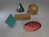
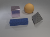
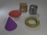
Image generation. We leverage the CLEVR [28] codebase to generate $160\times 120$ pixel color images, each image containing 4-5 objects that vary along three visual dimensions: shape, color, and texture. In each image, each object has a unique feature value on each dimension. We augmented CLEVR with additional features to ensure 10 values per dimension. (See supplementary material for details.) We synthesized 45,000 images for a training set, roughly balancing the count of each feature across images, and 5,000 for a hold-out set used to evaluate the model after each epoch and determine when to transition to the next episode. Each image could used for any task. Each epoch of training involved one pass through all images, with a random assignment of each image to a single task each epoch to satisfy the constraint on the distribution of tasks.

Tasks. For each replication of our simulation, we select one of the three dimensions and randomize the order of the ten within-dimension tasks. To reduce sensitivity of the results to the task order, we performed replications using a Latin square design [29, ch. 9], guaranteeing that within a block of ten replications, each task will appear in each ordinal position exactly once. We constructed six such Latin square blocks for each of the three dimensions (shape, color, and texture), resulting in 180 total simulation replications. Because we observed no meaningful qualitative differences across task dimensions (see supplementary material), the results we report below collapse across dimension.

Figure 2: Model architecture. Input consists of image and task representation. Dashed line from task representation to Conv-1 indicates optional task modulated visual processing, described under “Task-modulated visual processing.”

Figure 3: (a) Hold-out set accuracy as a function of training trials (log scale) for a newly introduced task. Colored lines indicate task ordinal position (cyan = introduced in episode 1; magenta = introduced in episode 10). In all panels, the shaded region represents $\pm 1$ standard error of the mean. (b) Hold-out accuracy of the task introduced in episode 1 by number of times it is retrained (black = 1 time, copper = 10 times). (c) Number of trials required to reach the accuracy criterion (log scale) as a function of the number of times a given task is trained (also log scale). As in (a), the colors indicate task ordinal position (the episode in which a task is introduced). (d) Similar to (c) but plotting only the new task introduced in a given episode. (e) Hold-out accuracy attained after a fixed amount of training (22.5k trials) of a given task, graphed as a function of number of times a given task is trained. As in (a), the colors indicate the episode in which a task is introduced. (f) Similar to (e) but plotting only the new task introduced in a given episode.

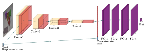
Architecture. Our experiments use a basic vision architecture with four convolutional layers followed by four fully connected layers (Figure 2). The convolutional layers—with 16, 32, 48, and 64 filters successively—each have 3x3 kernels with stride 1 and padding 1, followed by ReLU nonlinearities, batch normalization, and 2x2 max pooling. The fully-connected layers have 512 units in each, also with ReLU nonlinearities. All models were implemented in PyTorch [30] and trained with ADAM [31] using a learning rate of $0.0005$ and weight decay of $0.0001$. Note that our model is generic and is not specialized for metalearning or for preventing catastrophic forgetting. Instead of having one output head for each task, we specify the task as a component of the input. Similar to Sort-of-CLEVR [32], we code the task as a one-hot input vector. We concatenate the task representation to the output of the last convolutional layer before passing it to the first fully-connected layer. We verified this architecture has the capacity to learn all thirty tasks (in all three dimensions) when trained simultaneously (see Appendix A.3).

3 Results

3.1 Metalearning

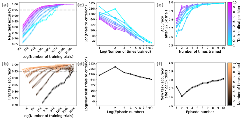
Figure 3a depicts hold-out accuracy for a newly introduced task as a function of the number of training trials. Curve colors indicate the task’s ordinal position in the series of episodes, with cyan being the first and magenta being the tenth. Not surprisingly, task accuracy improves monotonically over training trials. But notably, metalearning is evidenced because the accuracy of task $i+1$ is strictly higher than the accuracy of task $i$ for $i>2$. To analyze our simulations more systematically, we remind the reader that the simulation sequence presents fifty-five opportunities to assess learning: the task introduced in episode 1 (i.e., ordinal position 1) is trained ten times, the task introduced in episode 2 is trained nine times, and so forth, until the task introduced in episode 10, which is trained only once. Figure 3c indicates, with one line per task, the training required in a given episode to reach a hold-out accuracy of 95%—the dashed line in Figure 3a. Training required per episode is plotted as a function of the number of times the task is retrained. The downward shifting intercept of the curves for later tasks in the sequence indicates significantly easier learning and relearning. Figure 3e shows an alternative view of difficulty-of-training by plotting accuracy after a fixed amount of (re)training. The conditions that require the least number of trials to criterion (Figure 3c) also achieve the highest accuracy after a small amount of training (Figure 3e).

3.2 Catastrophic forgetting

Figure 3b shows the accuracy of the task introduced in the first episode ($y_{1}$) as it is retrained each episode. The fact that performance in a new episode drops below criterion (the dashed line) indicates backward interference. However, there is a relearning savings: the amount of interference diminishes monotonically with the number of times trained. Notably, catastrophic forgetting of task 1 is essentially eliminated by the last few episodes. Figure 3c shows very similar relearning savings for tasks 2-10 as for task 1. The roughly log-log linear curves offer evidence of power-law decrease in the retraining effort required to reach criterion.

Figure 3 also reveals that the first two episodes are anomalous. Strong backward interference on task 1 is exhibited when task 2 is introduced (the crossover of the cyan curve in Figure 3c), a phenomenon that does not occur for subsequent tasks. Similarly, strong forward interference on task 2 of task 1 is evident (slower learning for task 2 than for task 1 in Figure 3d), but tasks 3-10 are increasingly facilitated by previous learning. These findings suggest that to understand properties of neural nets, we must look beyond training on just two tasks, which is often the focus of research in transfer learning and catastrophic forgetting.

3.3 Resilience to forgetting

Figure 4: Exploration of forgetting. (a) Residual accuracy of task 1 as the task introduced in episodes 2-10 is trained (corresponding to 1-9 times that task 1 had previously been trained, with a black and copper for 1 and 9, respectively). (b) The inferred exponential decay rate as a function of the number of times a task is trained.

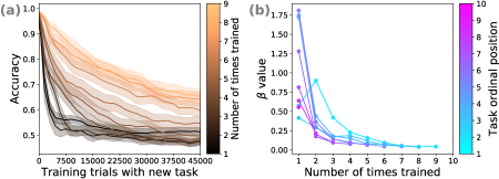
The fact that old tasks need to be retrained each episode suggests that training on a new task induces forgetting of the old. However, because we trained simultaneously on the old and new tasks, we have no opportunity to examine forgetting explicitly. Inspired by results from the human learning literature [33, 34], we hypothesized that the forgetting rate would decrease with additional training. We devised a setting to examine this hypothesis by cloning weights at various points in the simulation and examining a different training trajectory moving forward. We took the network weights at the start of each episode $i$, at which point the network is at criterion on tasks 1 through $i-1$. Then, instead of retraining on all $i$ tasks, we train only on task $i$. We probe the network regularly to evaluate residual performance on old tasks.

Figure 4a depicts the time course of forgetting of the task introduced in episode 1 on each subsequent episode. The black curve corresponds to episode 2 (task 1 has been trained only once previously) and the copper curve corresponds to episode 10 (task 1 has been trained 9 times previously). Task 1 becomes more robust to backward interference from the new task in later episodes, In episode $i$, task 1 has been (re)trained $i-1$ times previously, yielding a sort of spaced practice that appears to cause the memory to be more robust. This result is suggestive of the finding in human memory that interleaved, temporally distributed practice yields more robust and durable memory [35, 33].

Figure 4a depicts only some of the forty-five opportunities we have to assess forgetting: we have one after the model learns a single task, two after the model learns two, up to nine after the model learns the ninth task (for which we examine forgetting by training on the tenth and final task in the order). To conduct a more systematic analysis, we fit the forgetting curves for each task $i$ in each episode $e>i$. The forgetting curve characterizes accuracy $a$ after $t$ training batches of 1500 trials. Accuracy must be adjusted for guessing: because our tasks have a baseline correct-guessing rate of 0.5, we define $a=0.5+0.5m$, to be the observed accuracy when memory strength $m$ lies between 0 (no task memory) and 1 (complete and accurate task memory). We explore two characterizations of memory strength. The first is of exponential decay, $m=\alpha\exp(-\beta t)$, where $\alpha$ is the initial accuracy, $\beta$ is a decay rate, and $t$ is the number of intervening training batches. The second is of power-law decay, $m=\alpha(1+\gamma t)^{-\beta}$, where $\gamma$ serves as a timescale variable. This power-law decay curve is common in the psychological literature on forgetting [36] and has the virtue over $m=\alpha t^{-\beta}$ that it can characterize strength at $t=0$.

We fit the exponential and power-law functions separately to the data from each of the 45 model training points across 67 replications of our experiment. Following Clauset et al. [37], we fit each form to the first half of the data, and assess it on the second half of the data. The power-law function obtains a substantially lower MSE on the training data (power-law: 0.0045, exponential: 0.0198), the exponential function fit the held-out data better (power: 0.0232, exponential: 0.0192), and the exponential function offered a better fit on 24 of 45 training points of the model. We therefore adopt the exponential-decay function and characterize decay by rate parameter $\beta$.

Figure 4b presents the inferred decay rate $\beta$ for each of the forty-five model training points, presented in the style of Figures 3c,e. The basic pattern is clear: additional practice yields a more durable memory trace, regardless of a task’s ordinal position. Further, with the exception of tasks 1 and 2, the forgetting rate of task $i$ on episode $i+1$ decreases with $i$, One is tempted to interpret this effect in terms of studies of human long-term memory, where serial position effects are a robust phenomenon: Items learned early and late are preserved in memory better than items learned in between [38]. Psychological studies tend to train to people only once per task [e.g., 39] or multiple times on a single task [e.g., 40], so there are no behavioral data concerning how serial position interacts with number of times trained, as we have in the simulation. There are a number of respects in which our simulation methodology does not align with experimental methodology in psychological studies, such as the fact that we assess forgetting shortly after exposure, not at the end of a sequence of tasks. Nonetheless, the correspondence between our simulation and human memory is intriguing.

Figure 5: Heterogeneous task sequences. (a) Number of trials required to reach the accuracy criterion versus number of times a task is trained (cf. Figure 3c). The first two tasks are labeled by the numbers 1 and 2. (b) Increase in number of trials required to reach accuracy criterion for homogeneous sequences compared to heterogeneous as a baseline. Positive values indicate points learned faster in the heterogeneous condition, negative values in the baseline condition.

3.4 Heterogeneous task sequences

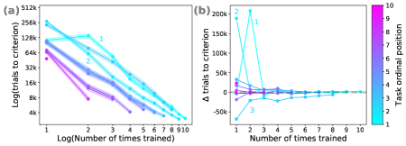
We noted two benefits of training on task sequences: reduced backward interference and increased forward facilitation. We next try to better understand the source of these benefits. In particular, we ask how the benefits relate to similarity among tasks. Previously, we sampled tasks homogeneously: all ten tasks in a sequence were drawn from a single dimension (color, shape, or texture). We now explore the consequence of sampling tasks heterogeneously: the ten tasks in a sequence draw from all three dimensions. Each replication utilizes a single permutation of the three dimensions and samples the ten tasks cycling between the dimensions (four from the first, three from the other two). We employed a similar Latin square design [29, ch. 9] to balance between the permutations, such that each block of six replications includes each permutation once.

Figure 5a presents the results of 114 replications of the heterogeneous sequences, nineteen using each of the six dimension permutations. To better compare to the homogeneous sequence results (Figure 3c), Figure 5b plots the increase in number of trials to criterion with homogeneous sequences compared to heterogeneous as a baseline. With several exception points, the differences are not notable, suggesting that inter-tasks effects with heterogeneous sequences are similar to those with homogeneous sequences. Thus, inter-task effects appear to be primarily due learning to process visual images in general, rather than the specific task-relevant dimensions. The two outlier points in Figure 5b concern the first two episodes: With heterogeneous training, the interference between tasks 1 and 2 nearly vanishes, perhaps because the resources and representations required to perform the two tasks overlap less. One might have predicted just the opposite result, but apparently, extracting information relevant for one visual dimension does not inhibit the construction of representations suitable for other dimensions. We argue that this finding is sensible given that the dimensions of color, form and texture are fundamentally confounded in the input image: interpreting color and texture can require information about an object’s shape, and vice-versa.

3.5 Task-modulated visual processing

The architecture that we have experimented with thus far treats the convolutional layers as visual feature extractors, trained end-to-end on task sequences, but the convolutional layers have no explicit information about task; task input is provided only to the final layers of the net. In contrast, processing in human visual cortex can be task modulated [41, 42]. Perhaps modifying the architecture to provide task information to convolutional layers would reduce inter-task interference. Along the lines of Mozer and Fan [43], we investigated a modified model using task-modulated visual processing, adopting a simpler approach than most existing architectures for conditional normalization or gated processing [44, 45]. We consider task modulation via a task-specific learned bias for each channel in a convolutional layer. As before, task is coded as a one-hot vector. We incorporate connections from the task representation to a convolutional layer (Figure 2), with one bias parameter for the Cartesian product of tasks and channels. This bias parameter is added to the output of each filter in a channel before applying the layer nonlinearity.

We investigated task modulation at each of the four convolutional layers in our model. Because the results of task modulation at the different layers are quite similar (see supplementary material), we report the results of modulating processing at the first convolutional layer. Figure 6 depicts the results of three Latin square replications, yielding thirty simulations for each dimension, or ninety in total. Introducing task-based modulation allows the model to avoid catastrophic forgetting previously observed from learning the second task on the first, and to a lesser effect, improves performance in the third episode as well. As the model learns additional tasks, and continues retraining on the same tasks, the benefits of task-modulation diminish rapidly (Figure 6b), suggesting the primary benefit is in aiding early learning. We hypothesize that modulating visual processing with the task representation allows the model to learn flexible visual representations that produce less interference.

Figure 6: Effect of modulating first convolutional layer with information about the current task. (a) Number of trials required to reach the accuracy criterion versus number of times a task is trained (cf. Figure 3c). (b) Increase in number of trials required to reach accuracy criterion for non-task-modulated versus task modulated architectures.

3.6 Comparison to MAML

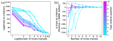
The results we have presented thus far serve as a baseline against which one can compare any method specialized to reduce forgetting or boost transfer. We conducted comparisons to several such methods, and in this section we report on experiments with model-agnostic metalearning or MAML [16]. MAML is designed to perform metalearning on a sequence of tasks in order to learn the next task in the sequence more efficiently. However, it is not designed for our continual-learning paradigm, which requires preservation of mastery for previous tasks. We explored two variants of MAML adapted to our paradigm. We report here on the more successful of the two (see supplementary material for details).

Our paradigm is based on a series of 10 episodes where tasks accumulate across episodes. MAML is also trained over a series of episodes, but we make a correspondence between one episode of MAML—the outer loop of the algorithm—and what we will refer to as a micro-episode of our paradigm, which corresponds to a single batch in our original training procedure. Each micro-episode starts with network weights ${\bm{w}}$, and we draw a half-batch of 750 examples (compared to 1500 in the original setting) of which 50% are from the newest task, and the remainder are split evenly across the previous tasks. (For task 1, all examples are from task 1.) From ${\bm{w}}$, we compute a gradient step based on the examples for each task, and apply this step separately to ${\bm{w}}$, yielding $i$ copies of the weights in episode $i$, $\{{\bm{w}}_{1},...,{\bm{w}}_{i}\}$, each specialized for its corresponding task. We then draw a second half-batch of 750 examples and perform a metatraining step, as described in MAML. Metatraining involves computing the gradient with respect to ${\bm{w}}$ for the new examples of each task $k$ based on the weights ${\bm{w}}_{k}$. Following MAML, we then update ${\bm{w}}$, and proceed to the next micro-episode until our training criterion is attained. Having halved the batch size, we doubled the learning rate from $0.0005$ in the original setting to $0.001$ for both of MAML’s learning rates. Model details are otherwise identical to the base model.

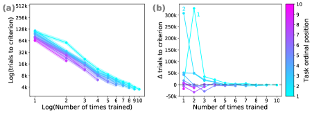
Over 90 replications (30 per dimensions), we find that the performance of our MAML variant is qualitatively similar to that of our base model (compare Figure 7a and Figure 3c). However, quantitatively, the MAML-based method requires more trials to reach criterion on expectation: Figure 7b shows the relative number of trials to criterion, where negative indicates that MAML is worse than our base model. Apparently the cost of splitting the data and devoting half to meta-training does not outweigh the benefit of meta-training.

Figure 7: MAML. (a) Number of trials (inner and outer loops combined) required to reach the accuracy criterion versus number of times a task is trained (cf. Figure 3c). (b) Increase in number of trials required to reach accuracy criterion for training without MAML compared to utilizing MAML. Negative values indicate slower learning with MAML than the base model.

4 Discussion

We explored the behavior of a standard convolutional neural net for classification in a continual-learning setting that introduces visual tasks sequentially and requires the net to master new tasks while preserving mastery of previously learned tasks. This setting corresponds to that which human learners naturally face as they become domain experts. For example, consider students reading a calculus text chapter by chapter. Early on, engaging with a chapter and its associated exercises results in forgetting of previously mastered material. However, as more knowledge is acquired, students begin to scaffold and link knowledge and eventually are able to integrate the new material with the old. As the final chapters are studied, students have built a strong conceptual framework which facilitates the integration of new material with little disruption of the old. These hypothetical students behave much like the net we studied in this article.

We summarize our novel findings, and where appropriate, we link these findings more concretely to the literature on human learning.

1. Metalearning (forward facilitation) is observed once the net has acquired sufficient domain expertise. In our paradigm, ‘sufficient expertise’ means having mastered two tasks previously. Metalearning is demonstrated when training efficiency—the number of trials needed to reach criterion—improves with each successive task (Figures 3d,f). Metalearning occurs naturally in the model and does not require specialized mechanisms. Indeed, incorporating a specialized mechanism, MAML, fails to enhance metalearning in our continual-learning paradigm.

2. Catastrophic forgetting (backward interference) is reduced as the net acquires increasing domain expertise (i.e., as more related tasks are learned). In Figure 3c, compare tasks introduced early (cyan) and late (magenta) in the sequence, matched for number of times they have been trained (position on the abscissa). Retraining efficiency improves for tasks introduced later in the task sequence, indicating a mitigation of forgetting. Note that the number of trials to relearn a skill is less than the number of trials required to initially learn a skill (the exception being task 1 in episode 2). This relearning savings effect has long been identified as a characteristic of human memory [46], as, of course, has the ubiquity of forgetting, whether due to the passage of time [47] or to backward interference from new knowledge [48].

3. The potential for catastrophic forgetting (backward interference) is also reduced each time a task is relearned, as indicated by the monotonically decreasing curves in Figure 3c and by the change in forgetting rates in Figure 4. A task that is practiced over multiple episodes receives distributed practice that is interleaved with other tasks. The durability of memory with distributed, interleaved practice is one of the most well studied phenomena in cognitive psychology [35, 33, 34, 49] and perceptual learning [50], helping human learners distinguish between categories, presumably by helping distinguish within- and between-category differences.

4. Training efficiency improves according to a power function of the number of tasks learned, controlling for experience on a task (indicated by the linear curve in Figure 3d, plotted in log-log coordinates), and also according to a power function of the amount of training a given task has received, controlling for number of tasks learned (indicated by the linear curves in Figure 3c). Power-law learning is a robust characteristic of human skill acquisition, observed on a range of behavioral measures [51, 52].

5. Forward facilitation and reduction in backward interference is observed only after two or more tasks have been learned. This pattern can be seen by the nonmonotonicities in the curves of Figures 3d,f and in the crossover of curves in Figures 3c,e. Catastrophic forgetting is evidenced primarily for task 1 when task 2 is learned—the canonical case studied in the literature. However, the net becomes more robust as it acquires domain expertise, and eventually the relearning effort becomes negligible (e.g., copper curves in Figure 3b). The anomalous behavior of task 2 is noteworthy, yielding a transition behavior perhaps analogous to the “zero-one-infinity” principle [53].

6. Catastrophic forgetting in the second episode can be mitigated in two different ways: first, by choosing tasks that rely on different dimensions (Figure 5); and second, by introducing task-based modulation of visual processing (Figure 6). We conjecture that both of these manipulations can be characterized in terms of reducing the similarity of the tasks. In human learning, reducing (semantic) similarity reduces interference [54], and top-down, task-based signals interplay with perceptual learning [55, 56], as early in processing as primary visual cortex (V1) [57, 58]. Our results imply that inter-task similarity creates higher levels interference for the first few tasks acquired, compared to training on a diverse set of tasks, without conferring additional benefits on facilitation of tasks introduced later. Consequently, training a model on diverse tasks might reduce forgetting without reducing forward facilitation. Task-based modulation serves as another promising avenue to reducing interference by similar tasks, which we hope to continue exploring in future work.

We are able to identify these intriguing phenomena because our simulations examined scaling behavior and not just effects of one task on a second—the typical case for studying catastrophic forgetting—or the effects of many tasks on a subsequent task—the typical case for metalearning and few-shot learning. Studying the continuum from the first task to the $n$’th is quite revealing.

We find that learning efficiency improves as more tasks are learned. Although MAML produces no benefit over the standard architecture that served as our baseline, we have yet to explore other methods that are explicitly designed to facilitate transfer and suppress interference [17, 12, 9]. The results presented in this article serve as a baseline to assess the benefits of specialized methods. A holy grail of sorts would be to identify methods that achieve backward facilitation, where training on later tasks improves performance on earlier tasks, and compositional generalization [59, 60, 61, 62], where learning the interrelationship among earlier tasks allows new tasks to be performed on the first trial. Humans demonstrate the former under rare conditions [63, 64]; the latter is common in human behavior, as when individuals are able to perform a task immediately from instruction.

An exciting direction for future research concerns optimizing curricula for continual learning. Our initial approach was inspired by best practices of the science of learning literature [65]. Our hope is that investigations of networks may in turn provide helpful guidance for improving curricula for human learners. Toward this goal, it is encouraging that we observed more than superficial similarities between human and network continual learning.

Appendix A Supplementary materials

A.1 Feature values

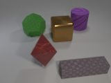
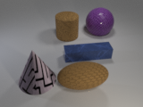
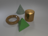
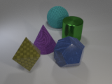
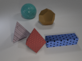
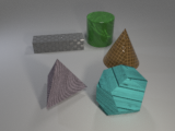
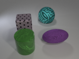
The ten colors used in our experiments are: gray, red, blue, green, brown, purple, magenta, yellow, orange, pink. The ten shapes are: cube, sphere, cylinder, pyramid, cone, torus, rectangular box, ellipsoid, octahedron, dodecahedron. And the ten textures are: metal, rubber, chainmail, marble, maze, metal weave, polka dots, rug, bathroom tiles, wooden planks. See additional example images below:

Figure 8: Additional example training images

A.2 Curriculum ablations

To explore the sensitivity of our results to our formulation of the coreset as a curriculum, we devised two alternative approaches, beyond the baseline approach reported of allocating half of the examples in each epoch to the newest task, and splitting the remaining examples evenly between previously learned tasks. With all curricula explored below, we make an effort to attain the same balance both within each epoch as a whole, and within each batch in the epoch. We also maintained the same evaluation protocol as with the baseline curriculum to make sure the results are comparable.

A.2.1 Ratio curriculum

In this curriculum, we again allocate half of the examples in each epoch to the newest task. We split the remaining half such that the ratio between examples allocated to task $k$ and task $k+1$ is $1:\kappa$, where $\kappa\geq 1$ is a free parameter. This allows newer tasks, which the model learned fewer times, to receive proportionally more instruction than previous tasks. Note that for the first two episodes, this behaves identically to the baseline curriculum we investigated. We explored two settings of $\kappa$: the first, $\kappa=1.24$, we approximated from the data collected under our baseline curriculum, and a second, $\kappa=1.5$, we chose to explore the sensitivity to this parameter.

For example, with $\kappa=1.25$, the third episode, the first task receives 10000 examples, the second 12500, and the third, and newest task, receives its 22500 examples in each epoch. For another example, in the sixth episode, the tasks are allocated the following numbers of examples per epoch: 2741, 3427, 4284, 5355, 6693, and 22500. With $\kappa=1.5$, the third episode allocations are 9000, 13500, and 22500, and the sixth episode training example allocations are 1706, 2559, 3839, 5758, 8638, and 22500.

A.2.2 Power curriculum

In this curriculum, unlike the baseline and the ratio curriculum we omit the allocation of half of the examples to the newest task. In episode $k$, for task $1,2,\ldots t,\ldots,k$, we first compute unnormalized proportions using a power function: task 1 receives $\rho_{1}=k^{-\alpha}$, task 2 receives $\rho_{2}={k-1}^{-\alpha}$, and so on, such that each task $t$ receives a proportion of $\rho_{t}=(k-t+1)^{-\alpha}$ of the examples. We then normalize the proportions, such that each task receives $p_{t}=\frac{\rho_{t}}{\sum_{i=1}^{k}\rho_{i}}$ of the 45000 total training examples per epoch. As with the ratio curriculum, we first estimated $\alpha$ from the baseline curriculum data, arriving at $\alpha=1.14$, and then explored an alternative setting of $\alpha=2$. For example, with $\alpha=1.14$, in the third episode, task 1 receives 7394 training examples, task 2 receives 11738 examples, and task 3 (the newest task) receives 25868 examples. In the sixth episode, tasks 1-6 are allocated the following numbers of examples: 2611, 3215, 4146, 5755, 9137, and 20136. With $\alpha=2$, in the third episode we allocate 3674, 8265, and 33061 training examples to tasks 1-3 respectively, and in the six episode, we allocate tasks 1-6 838, 1207, 1886, 3353, 7543, and 30173 training examples respectively.

A.2.3 Results

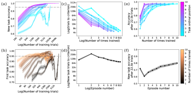
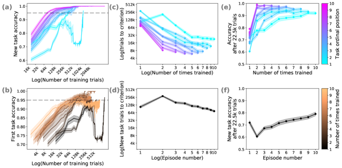
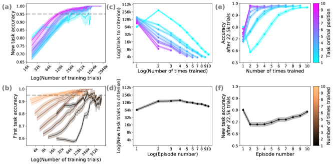
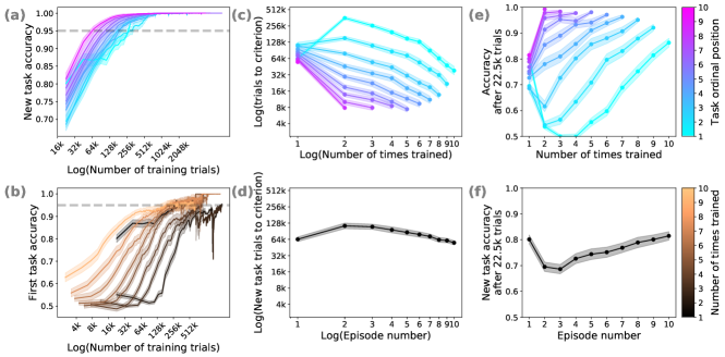
We reproduced Figure 3 with the data from running two Latin square replications in each dimension (resulting in sixty total runs) utilizing each curriculum. The results in panels (a) and (b) are noisier, especially for above 256k examples, as most runs finish sooner, and thus there is less data in in that part of the plot. Qualitative, we find panels (c)-(f) quite similar to the baseline curriculum, especially for the two data-optimized versions of the curriculum (Figure 9 and Figure 11), and slightly less so for the misspecified versions (Figure 10 and Figure 12).

Figure 9: Reproduction of Figure 3 with the data from the ratio curriculum using a ratio of $\kappa=1.25$ approximated from the baseline curriculum data.

Figure 10: Reproduction of Figure 3 with the data from the ratio curriculum using a ratio of $\kappa=1.5$ designed to explore the sensitivity to the choice of parameter.

Figure 11: Reproduction of Figure 3 with the data from the power curriculum using an exponent of $\alpha=1.14$ approximated from the baseline curriculum data.

Figure 12: Reproduction of Figure 3 with the data from the power curriculum using an exponent of $\alpha=2$ designed to explore the sensitivity to the choice of parameter.

A.3 Simultaneous training architecture capacity

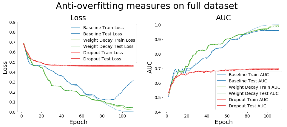
We compared a few variations on our model architecture to validate it has the capacity to learn these tasks when trained simultaneously. The loss and AUC curves plotted below provide results from a baseline model, a model with dropout, and the model reported in the paper, which utilizes weight decay but not dropout.

Figure 13: Loss and AUC curves for architecture variants when training on all thirty tasks simultaneously.

A.4 Results by dimension

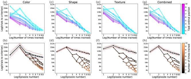
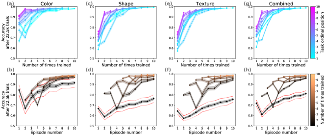
To justify our collapsing of the results across dimensions, we provide the results broken down for each individual dimension below. Figure 14 depicts the trials required to reach the accuracy criterion, Figure 14g,h reproducing Figure 3c,d, and the rest of the subfigures offering the results for replications within each dimension. While colors are easier to learn than shapes or textures, simulations in all three dimensions show the same qualitative features. Similarly, Figure 15 depicts the accuracy after a fixed small amount of training, with Figure 15g,h reproducing Figure 3e,f. These results provide further evidence for the ease of learning color compared to the other two dimensions, but the qualitative similarity remains striking.

Figure 14: (a, c, e, g): Number of trials required to reach the accuracy criterion (log scale) as a function of the number of times a given task is trained (also log scale). The colored lines indicate task ordinal position (cyan = introduced in episode 1; magenta = introduced in episode 10). (b, d, f, h): Number of trials required to reach the accuracy criterion (log scale) as a function of the episode number. The colored lines indicate the number of times a task was retrained on (black = 1 time, copper = 10 times). In all panels, the shaded region represents $\pm 1$ standard error of the mean.

Figure 15: (a, c, e, g): Accuracy after a fixed amount of training (22,500 trials) as a function of the number of times a given task is trained (log scale). The colored lines indicate task ordinal position (cyan = introduced in episode 1; magenta = introduced in episode 10). (b, d, f, h): Accuracy after the same fixed amount of training as a function of the episode number. The colored lines indicate the number of times a task was retrained on (black = 1 time, copper = 10 times). In all panels, the shaded region represents $\pm 1$ standard error of the mean.

A.5 Task-modulated processing at different levels

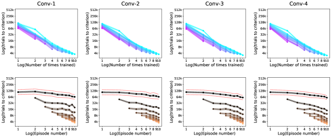
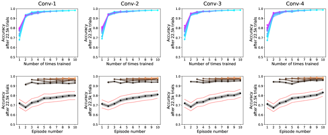
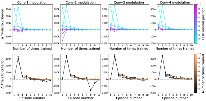
All figures reported below are combined over replications in all three dimensions, where for each modulation level we performed thirty simulations in each dimension, yielding ninety simulations in total for each modulation level. In Figure 16, we provide the results plotted in Figure 5a-b for task-modulation at each convolutional layer (separately). In Figure 17, we provide equivalent plots to Figure 2e-f for the task-modulated models. In Figure 18, we provide equivalent plots to Figure 5c-d for the task-modulated models. The only anomaly we observe is in Figure 18 for task-modulation at the second convolutional layer, where the eight and ninth tasks appear easier to learn for the first time without task-modulation. Save for this anomaly, we observed remarkably consistent results between the different modulation levels, and hence we reported a single one, rather than expanding about all four.

Figure 16: Top panels: Number of trials required to reach the accuracy criterion (log scale) as a function of the number of times a given task is trained (also log scale). The colors indicate task ordinal position (the episode in which a task is introduced; cyan = introduced in episode 1; magenta = introduced in episode 10). Bottom panels: Similar to the top panels, but graphed as a function of episode number with the line colors indicating the number of times a task is retrained (black = 1 time, copper = 10 times).

Figure 17: Top panels: Hold-out accuracy attained after a fixed amount of training (22.5k trials) of a given task, graphed as a function of number of times a given task is trained. As in Figure 16, the colors indicate task ordinal position (the episode in which a task is introduced; cyan = introduced in episode 1; magenta = introduced in episode 10). Bottom panels: Similar to the top panels, but graphed as a function of episode number with the line colors indicating–as in Figure 16–the number of times a task is retrained (black = 1 time, copper = 10 times).

Figure 18: Top panels: Increase in number of trials required to reach accuracy criterion for non-task-modulated versus task modulated architectures as a function of the number of times a given task is trained (also log scale). The colors indicate task ordinal position (the episode in which a task is introduced; cyan = introduced in episode 1; magenta = introduced in episode 10). Bottom panels: Similar to the top panels, but graphed as a function of episode number with the line colors indicating the number of times a task is retrained (black = 1 time, copper = 10 times).

A.6 MAML comparison supplement

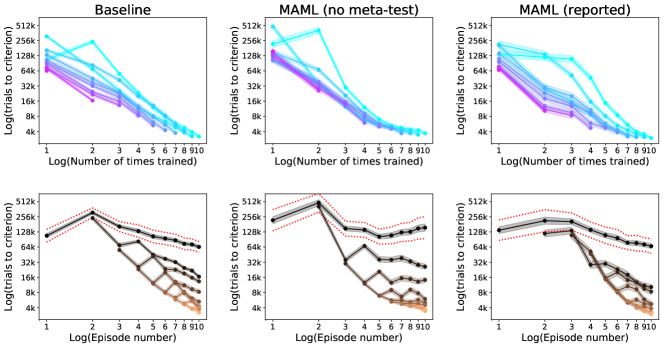
We compared our baseline model to two versions of MAML. Both utilized the training procedure we describe under the ‘Comparison to MAML’ section. The first, reported in the middle column below, only utilized this procedure in training, and was tested without the meta-testing step. In other words, this model was tested exactly as our baseline model was tested, to see if MAML manages to learn representations that allow it to answer questions on unseen images without further adaptation. The second version, which we ended up reporting, also utilizes the micro-episode procedure at test time, making train and test identical. The results below demonstrate similar qualitative behavior between our baseline and both versions. However, as the second version, using the meta-testing procedure, fares better, we opt to report it in the submission.

Figure 19: MAML comparison. The left column plots result from our baseline condition. The middle column offers results from a version of MAML which did not follow the micro-episode procedure at test that, that is, did not meta-test. The right column, corresponding to the model reported in the submission, follows the micro-episode procedure we describe at both train and test.

A.7 Comparison to simultaneous learning

We performed a systematic comparison between our sequential method of training and the standard supervised learning approach of training on all tasks simultaneously. We know that sequential training is beneficial to humans–every course covers one topic at a time, rather than throwing the entire textbook and mixing all topics from day one. There is also ample evidence for the value of curricular approaches in machine learning, going as far back as [66]. However, curricula in machine learning usually attempt to scaffold tasks from smaller to larger, or easier to harder, following some difficulty gradient. Our results in Figure 20 suggest, surprisingly, that randomly chosen sequential curriculum (that is, random task introduction orderings) can significantly speed up learning in some cases. We find, interestingly, that this effect varies by dimension. While in the shape condition the simultaneous learning is competitive with sequential training, we find that in both texture and color sequential training proceeds much faster. In those cases, the number of training trials required to learn each task when trained sequentially (the cyan-to-magenta curves) is far less than the number of trials required to learn each task when trained simultaneously (the red curve). That is, task $n+1$ is learned far faster following tasks 1–$n$ than simultaneously with tasks 1–10. The long plateau in the color and texture cases appears to suggest some form of initial representation learning which is made more efficient by learning sequentially, rather than simultaneously.

Figure 20: Simultaneous vs. sequential training. The cyan (first) to magenta (last) colored lines plot the accuracy after some number of training trials for each task the model learned. The average accuracy over all ten tasks, when learned simultaneously, is plotted in red. To make the comparisons valid, the simultaneous training is in the number of training trials for each task, rather than combined for all tasks.

References

- Caruana [1997] R. Caruana, “Multitask Learning,” Machine Learning, vol. 28, pp. 41–75, 1997.
- Caruana [1993] ——, “Multitask learning: A knowledge-based source of inductive bias,” in Proceedings of the Tenth International Conference on Machine Learning. Morgan Kaufmann, 1993, pp. 41–48.
- Ruder [2017] S. Ruder, “An Overview of Multi-Task Learning in Deep Neural Networks,” arXiv, Tech. Rep., Jun 2017. [Online]. Available: https://arxiv.org/abs/1807.07545
- Thrun [1996] S. Thrun, “Is Learning The n-th Thing Any Easier Than Learning The First?” in Advances in Neural Information Processing Systems 8, D. S. Touretzky, M. C. Mozer, and M. E. Hasselmo, Eds. MIT Press, 1996, pp. 640–646.
- Parisi et al. [2019] G. I. Parisi, R. Kemker, J. L. Part, C. Kanan, and S. Wermter, “Continual lifelong learning with neural networks: A review,” Neural Networks, vol. 113, pp. 54–71, may 2019. [Online]. Available: https://www-sciencedirect-com.ccl.idm.oclc.org/science/article/pii/S0893608019300231https://arxiv.org/pdf/1802.07569.pdf
- McCloskey and Cohen [1989] M. McCloskey and N. J. Cohen, “Catastrophic Interference in Connectionist Networks: The Sequential Learning Problem,” Psychology of Learning and Motivation, vol. 24, pp. 109–165, jan 1989. [Online]. Available: https://www-sciencedirect-com.ccl.idm.oclc.org/science/article/pii/S0079742108605368
- Schmidhuber [1987] J. Schmidhuber, “Evolutionary Principles in Self-Referential Learning,” Ph.D. dissertation, TU Munich, 1987. [Online]. Available: http://people.idsia.ch/{~}juergen/diploma1987ocr.pdf
- Bengio et al. [1991] Y. Bengio, S. Bengio, and J. Cloutier, “Learning a synaptic learning rule,” in Seattle International Joint Conference on Neural Networks, vol. ii. IEEE, 1991, p. 969. [Online]. Available: http://ieeexplore.ieee.org/document/155621/
- Lopez-Paz and Ranzato [2017] D. Lopez-Paz and M. . A. Ranzato, “Gradient Episodic Memory for Continual Learning,” in NIPS, 2017. [Online]. Available: https://github.com/
- Schwarz et al. [2018] J. Schwarz, J. Luketina, W. M. Czarnecki, A. Grabska-Barwinska, Y. W. Teh, R. Pascanu, and R. Hadsell, “Progress & Compress: A scalable framework for continual learning,” in Proceedings of the 35th International Conference on Machine Learning, may 2018, pp. PMLR 80:4528–4537. [Online]. Available: http://arxiv.org/abs/1805.06370
- Goodfellow et al. [2015] I. J. Goodfellow, M. Mirza, D. Xiao, A. Courville, and Y. Bengio, “An Empirical Investigation of Catastrophic Forgetting in Gradient-Based Neural Networks,” 2015. [Online]. Available: http://arxiv.org/abs/1312.6211
- Kirkpatrick et al. [2017] J. Kirkpatrick, R. Pascanu, N. Rabinowitz, J. Veness, G. Desjardins, A. A. Rusu, K. Milan, J. Quan, T. Ramalho, A. Grabska-Barwinska, D. Hassabis, C. Clopath, D. Kumaran, and R. Hadsell, “Overcoming catastrophic forgetting in neural networks,” Proceedings of the National Academy of Sciences, vol. 114, no. 13, pp. 3521–3526, 2017. [Online]. Available: https://www.pnas.org/content/114/13/3521
- Zenke et al. [2017] F. Zenke, B. Poole, and S. Ganguli, “Continual Learning Through Synaptic Intelligence,” in ICML, 2017. [Online]. Available: https://arxiv.org/pdf/1703.04200.pdf
- Kamra et al. [2017] N. Kamra, U. Gupta, and Y. Liu, “Deep Generative Dual Memory Network for Continual Learning,” oct 2017. [Online]. Available: http://arxiv.org/abs/1710.10368
- Kemker and Kanan [2018] R. Kemker and C. Kanan, “FearNet: Brain-Inspired Model for Incremental Learning,” in ICLR, nov 2018. [Online]. Available: http://arxiv.org/abs/1711.10563
- Finn et al. [2017] C. Finn, P. Abbeel, and S. Levine, “Model-Agnostic Meta-Learning for Fast Adaptation of Deep Networks,” Proceedings of the 34th International Conference on Machine Learning,, vol. 70, 2017. [Online]. Available: https://arxiv.org/pdf/1703.03400.pdf
- Mishra et al. [2018] N. Mishra, M. Rohaninejad, X. Chen, and P. Abbeel, “A Simple Neural Attentive Meta-Learner,” in International Conference on Learning Representations, 2018. [Online]. Available: https://arxiv.org/pdf/1707.03141.pdf
- Andrychowicz et al. [2016] M. Andrychowicz, M. Denil, S. Gomez, M. W. Hoffman, D. Pfau, T. Schaul, B. Shillingford, and N. de Freitas, “Learning to learn by gradient descent by gradient descent,” Advances in Neural Information Processing Systems 29, pp. 3981–3989, jun 2016. [Online]. Available: http://arxiv.org/abs/1606.04474
- Wang et al. [2017] J. X. Wang, Z. Kurth-Nelson, D. Tirumala, H. Soyer, J. Z. Leibo, R. Munos, C. Blundell, D. Kumaran, and M. Botvinick, “Learning to Reinforcement Learn,” in CogSci. DeepMind, 2017. [Online]. Available: https://arxiv.org/pdf/1611.05763v3.pdf
- [20] Y. LeCun, C. Cortes, and C. Burges, “MNIST handwritten digit database.” [Online]. Available: http://yann.lecun.com/exdb/mnist/
- Welinder et al. [2010] P. Welinder, S. Branson, T. Mita, C. Wah, F. Schroff, S. Belongie, and P. Perona, “Caltech-UCSD Birds 200,” California Institute of Technology, Tech. Rep. CNS-TR-2010-001, 2010.
- Lomanco and Maltoni [2017] V. Lomanco and D. Maltoni, “Core50: a new dataset and benchmark for continual object recognition,” in Proceedings of the 1st Annual Conference on Robot Learning, 2017, pp. 17–26. [Online]. Available: http://proceedings.mlr.press/v78/lomonaco17a.html
- Lomanco et al. [2019] V. Lomanco, D. Maltoni, and L. Pellegrini, “Fine-Grained Continual Learning ,” arXiv, Tech. Rep., Jul 2019. [Online]. Available: https://arxiv.org/abs/1907.03799
- Lee et al. [2019] K. Lee, K. Lee, J. Shin, and H. Lee, “Overcoming catastrophic forgetting with unlabeled data in the wild,” in ICCV, 2019.
- Aljundi et al. [2019] R. Aljundi, K. Kelchtermans, and T. Tuytelaars, “Task-Free Continual Learning,” in Proceedings of the IEEE Computer Society Conference on Computer Vision and Pattern Recognition (CVPR), aug 2019. [Online]. Available: http://arxiv.org/abs/1812.03596
- Stojanov et al. [2019] S. Stojanov, S. Mishra, N. A. Thai, N. Dhanda, A. Humayun, C. Yu, L. B. Smith, and J. M. Rehg, “Incremental object learning from contiguous views,” in The IEEE Conference on Computer Vision and Pattern Recognition (CVPR), June 2019.
- Nguyen et al. [2018] C. V. Nguyen, Y. Li, T. D. Bui, and R. E. Turner, “Variational Continual Learning,” ICLR, oct 2018. [Online]. Available: http://arxiv.org/abs/1710.10628
- Johnson et al. [2017] J. Johnson, L. Fei-Fei, B. Hariharan, C. L. Zitnick, L. Van Der Maaten, and R. Girshick, “CLEVR: A Diagnostic Dataset for Compositional Language and Elementary Visual Reasoning,” in Proceedings of the IEEE Computer Society Conference on Computer Vision and Pattern Recognition (CVPR), 2017. [Online]. Available: https://arxiv.org/pdf/1612.06890.pdf
- Bailey [2008] R. Bailey, Design of comparative experiments, 1st ed. Cambridge University Press, 2008.
- Paszke et al. [2017] A. Paszke, S. Gross, S. Chintala, G. Chanan, E. Yang, Z. DeVito, Z. Lin, A. Desmaison, L. Antiga, and A. Lerer, “Automatic differentiation in PyTorch,” in NIPS, 2017.
- Kingma and Ba [2015] D. P. Kingma and J. Ba, “Adam: A Method for Stochastic Optimization,” in Proceedings of the 3rd International Conference for Learning Representations, 2015. [Online]. Available: https://arxiv.org/abs/1412.6980
- Santoro et al. [2017] A. Santoro, D. Raposo, D. G. T. Barrett, M. Malinowski, R. Pascanu, P. Battaglia, T. Lillicrap, and D. London, “A simple neural network module for relational reasoning,” in Advances in Neural Information Processing Systems 30, I. Guyon, U. V. Luxburg, S. Bengio, H. Wallach, R. Fergus, S. . Vishwanathan, and R. Garnett, Eds. Curran Associates, Inc., 2017, pp. 4967–4976. [Online]. Available: https://arxiv.org/pdf/1706.01427.pdf
- Cepeda et al. [2008] N. J. Cepeda, E. Vul, D. Rohrer, J. T. Wixted, and H. Pashler, “Spacing effects in learning: A temporal ridgeline of optimal retention,” Psychological Science, vol. 19, pp. 1095–1102, 2008.
- Taylor and Rohrer [2010] K. Taylor and D. Rohrer, “The effects of interleaved practice,” Applied Cognitive Psychology, vol. 24, no. 6, pp. 837–848, sep 2010. [Online]. Available: http://doi.wiley.com/10.1002/acp.1598
- Kang et al. [2014] S. H. K. Kang, R. V. Lindsey, M. C. Mozer, and H. Pashler, “Retrieval practice over the long term: Expanding or equal-interval spacing?” Psychological Bulletin & Review, vol. 21, pp. 1544–1550, 2014.
- Wixted and Carpenter [2007] J. T. Wixted and S. K. Carpenter, “The Wickelgren power law and the ebbinghaus savings function,” Psychological Science, vol. 18, pp. 133–134, 2007.
- Clauset et al. [2009] A. Clauset, C. Shalizi, and M. Newman, “Power-law distributions in empirical data,” SIAM Review, vol. 51, no. 4, pp. 661–703, 2009.
- Glenberg et al. [1980] A. M. Glenberg, M. M. Bradley, J. A. Stevenson, T. A. Kraus, M. J. Tkachuk, A. L. Gretz, and B. M. Turpin, “A two-process account of long-term serial position effects,” Journal of Experimental Psychology: Human Learning and Memory, vol. 6, no. 4, pp. 355–369, 1980.
- Neumann and Ammons [1957] E. Neumann and R. B. Ammons, “Acquisition and long-term retention of a simple serial perceptual-motor skill.” Journal of Experimental Psychology, vol. 53, no. 3, pp. 159–161, 1957.
- Gerson and Thomas [1978] R. F. Gerson and J. R. Thomas, “A neo-Piagetian investigation of the serial position effect in children’s motor learning,” Journal of Motor Behavior, vol. 10, no. 2, pp. 95–104, 1978, pMID: 15180912. [Online]. Available: https://doi.org/10.1080/00222895.1978.10735142
- Fias et al. [2002] W. Fias, P. Dupont, B. Reynvoet, and G. A. Orban, “The quantitative nature of a visual task differentiates between ventral and dorsal stream,” Journal of Cognitive Neuroscience, vol. 14, pp. 646–658, 2002.
- Bracci et al. [2017] S. Bracci, N. Daniels, and H. Op de Beeck, “Task Context Overrules Object- and Category-Related Representational Content in the Human Parietal Cortex.” Cerebral cortex (New York, N.Y. : 1991), vol. 27, no. 1, pp. 310–321, 2017. [Online]. Available: http://www.ncbi.nlm.nih.gov/pubmed/28108492http://www.pubmedcentral.nih.gov/articlerender.fcgi?artid=PMC5939221
- Mozer and Fan [2008] M. C. Mozer and A. Fan, “Top-Down modulation of neural responses in visual perception: a computational exploration,” Natural Computing, vol. 7, no. 1, pp. 45–55, mar 2008. [Online]. Available: http://link.springer.com/10.1007/s11047-007-9041-0
- Perez et al. [2018] E. Perez, F. Strub, H. de Vries, V. Dumoulin, and A. Courville, “FiLM: Visual Reasoning with a General Conditioning Layer,” in AAAI’18, sep 2018. [Online]. Available: http://arxiv.org/abs/1709.07871
- Chen et al. [2018] Z. Chen, Y. Li, S. Bengio, and S. Si, “GaterNet: Dynamic filter selection in convolutional neural network via a dedicated global gating network,” arXiv, Tech. Rep., 2018. [Online]. Available: https://arxiv.org/pdf/1811.11205.pdf
- Ebbinghaus [1908] H. Ebbinghaus, Psychology: An elementary textbook. Arno Press, 1908.
- Lindsey et al. [2014] R. V. Lindsey, J. D. Shroyer, H. Pashler, and M. C. Mozer, “Improving Students’ Long-Term Knowledge Retention Through Personalized Review,” Psychological Science, vol. 25, no. 3, pp. 639–647, mar 2014.
- Osgood [1948] C. E. Osgood, “An investigation into the causes of retroactive interference.” Journal of Experimental Psychology, vol. 38, no. 2, pp. 132–154, 1948. [Online]. Available: http://doi.apa.org/getdoi.cfm?doi=10.1037/h0055753
- Birnbaum et al. [2013] M. S. Birnbaum, N. Kornell, E. L. Bjork, and R. A. Bjork, “Why interleaving enhances inductive learning: The roles of discrimination and retrieval,” Memory & Cognition, vol. 41, no. 3, pp. 392–402, apr 2013. [Online]. Available: http://www.ncbi.nlm.nih.gov/pubmed/23138567http://link.springer.com/10.3758/s13421-012-0272-7
- Szpiro et al. [2014] S. F. A. Szpiro, B. A. Wright, and M. Carrasco, “Learning one task by interleaving practice with another task.” Vision research, vol. 101, pp. 118–24, aug 2014.
- Newell and Rosenbloom [1980] A. Newell and P. S. Rosenbloom, “Mechanisms of Skill Acquisition and the Law of Practice.” in Cognitive Skills and their Acquisition, 1st ed., J. R. Anderson, Ed. Erlbaum, 1980. [Online]. Available: https://apps.dtic.mil/docs/citations/ADA096527
- Donner and Hardy [2015] Y. Donner and J. L. Hardy, “Piecewise power laws in individual learning curves,” Psychonomic Bulletin & Review, vol. 22, no. 5, pp. 1308–1319, oct 2015. [Online]. Available: http://link.springer.com/10.3758/s13423-015-0811-x
- MacLennan [1999] B. J. MacLennan, Principles of Programming Languages (3rd Ed.): Design, Evaluation, and Implementation. New York, NY, USA: Oxford University Press, Inc., 1999.
- Baddeley and Dale [1966] A. D. Baddeley and C. A. Dale, “The effect of semantic similarity on retroactive interference in long- and short-term memory,” Journal of Verbal Learning and Verbal Behavior, vol. 5, pp. 417–420, 1966.
- Seitz et al. [2005] A. R. Seitz, N. Yamagishi, B. Werner, N. Goda, M. Kawato, and T. Watanabe, “Task-specific disruption of perceptual learning,” Proceedings of the National Academy of Sciences of the United States of America, vol. 102, no. 41, pp. 14 895–14 900, oct 2005.
- Byers and Serences [2012] A. Byers and J. T. Serences, “Exploring the relationship between perceptual learning and top-down attentional control,” Vision Research, vol. 74, pp. 30–39, dec 2012.
- Li et al. [2004] W. Li, V. Piëch, and C. D. Gilbert, “Perceptual learning and top-down influences in primary visual cortex,” Nature Neuroscience, vol. 7, no. 6, pp. 651–657, jun 2004.
- Schäfer et al. [2007] R. Schäfer, E. Vasilaki, and W. Senn, “Perceptual Learning via Modification of Cortical Top-Down Signals,” PLoS Computational Biology, vol. 3, no. 8, p. e165, 2007. [Online]. Available: https://dx.plos.org/10.1371/journal.pcbi.0030165
- Fodor and Pylyshyn [1988] J. A. Fodor and Z. W. Pylyshyn, “Connectionism and cognitive architecture: a critical analysis.” Cognition, vol. 28, no. 1-2, pp. 3–71, mar 1988. [Online]. Available: http://www.ncbi.nlm.nih.gov/pubmed/2450716
- Fodor and Lepore [2002] J. A. Fodor and E. Lepore, Compositionality Papers. Oxford University Press UK, 2002.
- Lake and Baroni [2018] B. Lake and M. Baroni, “Generalization without systematicity: On the compositional skills of sequence-to-sequence recurrent networks,” in Proceedings of the 35th International Conference on Machine Learning, ser. Proceedings of Machine Learning Research, J. Dy and A. Krause, Eds., vol. 80. Stockholmsmässan, Stockholm Sweden: PMLR, 10–15 Jul 2018, pp. 2873–2882. [Online]. Available: http://proceedings.mlr.press/v80/lake18a.html
- Loula et al. [2018] J. Loula, M. Baroni, and B. Lake, “Rearranging the Familiar: Testing Compositional Generalization in Recurrent Networks,” arXiv, Tech. Rep., jul 2018. [Online]. Available: https://arxiv.org/abs/1807.07545
- Ausubel et al. [1957] D. P. Ausubel, L. C. Robbins, and J. Blake, Elias, “Retroactive inhibition and facilitation in the learning of school materials.” Journal of Educational Psychology, vol. 48, no. 6, pp. 334–343, 1957. [Online]. Available: http://content.apa.org/journals/edu/48/6/334
- Jacoby et al. [2015] L. L. Jacoby, C. N. Wahlheim, and C. M. Kelley, “Memory consequences of looking back to notice change: Retroactive and proactive facilitation.” Journal of Experimental Psychology: Learning, Memory, and Cognition, vol. 41, no. 5, pp. 1282–1297, sep 2015. [Online]. Available: http://www.ncbi.nlm.nih.gov/pubmed/26010827http://doi.apa.org/getdoi.cfm?doi=10.1037/xlm0000123
- Weinstein et al. [2018] Y. Weinstein, C. R. Madan, and M. A. Sumeracki, “Teaching the science of learning.” Cognitive research: principles and implications, vol. 3, no. 1, p. 2, 2018.
- Elman [1993] J. L. Elman, “Learning and development in neural networks: the importance of starting small,” Cognition, vol. 48, no. 1, pp. 71–99, jul 1993. [Online]. Available: https://www.sciencedirect.com/science/article/pii/0010027793900584http://citeseerx.ist.psu.edu/viewdoc/download?doi=10.1.1.128.4487{&}rep=rep1{&}type=pdf