Regularity as Regularization:
Smooth and Strongly Convex Brenier Potentials in Optimal Transport


François-Pierre Paty                        Alexandre d’Aspremont                        Marco Cuturi

CREST, ENSAE, Institut Polytechnique de Paris                        CNRS, ENS, PSL Research University                        Google Brain, CREST, ENSAE

Abstract

Estimating Wasserstein distances between two high-dimensional densities suffers from the curse of dimensionality: one needs an exponential (wrt dimension) number of samples to ensure that the distance between two empirical measures is comparable to the distance between the original densities. Therefore, optimal transport (OT) can only be used in machine learning if it is substantially regularized. On the other hand, one of the greatest achievements of the OT literature in recent years lies in regularity theory: Caffarelli (2000) showed that the OT map between two well behaved measures is Lipschitz, or equivalently when considering 2-Wasserstein distances, that Brenier convex potentials (whose gradient yields an optimal map) are smooth. We propose in this work to draw inspiration from this theory and use regularity as a regularization tool. We give algorithms operating on two discrete measures that can recover nearly optimal transport maps with small distortion, or equivalently, nearly optimal Brenier potentials that are strongly convex and smooth. The problem boils down to solving alternatively a convex QCQP and a discrete OT problem, granting access to the values and gradients of the Brenier potential not only on sampled points, but also out of sample at the cost of solving a simpler QCQP for each evaluation. We propose algorithms to estimate and evaluate transport maps with desired regularity properties, benchmark their statistical performance, apply them to domain adaptation and visualize their action on a color transfer task.

1 INTRODUCTION

Optimal transport (OT) has found practical applications in areas as diverse as supervised machine learning (Frogner et al., 2015; Abadeh et al., 2015; Courty et al., 2016), graphics (Solomon et al., 2015; Bonneel et al., 2016), generative models (Arjovsky et al., 2017; Salimans et al., 2018), NLP (Grave et al., 2019; Alaux et al., 2019), biology (Hashimoto et al., 2016; Schiebinger et al., 2019) or imaging (Rabin & Papadakis, 2015; Cuturi & Peyré, 2016). OT theory is useful in these applications because it provides tools that can quantify the closeness between probability measures even when they do not have overlapping supports, and more generally because it defines tools to infer maps that can push-forward (or morph) one measure onto another. There is, however, an important difference between the OT definitions introduced in celebrated textbooks by Villani (2003; 2009) and Santambrogio (2015), and those used in the works cited above. In all of these applications, some form of regularization is used to ensure that computations are not only tractable but also meaningful, in the sense that the naive implementation of linear programs to solve OT on discrete histograms/measures are not only too costly but also suffer from the curse of dimensionality (Dudley, 1969; Panaretos & Zemel, 2019). Regularization, defined explicitly or implicitly as an approximation algorithm, is therefore crucial to ensure that OT is meaningful and can work at scale.

Brenier Potentials and Regularity Theory. In the OT literature, regularity has a different meaning, one that is usually associated with the properties of the optimal Monge map (Villani, 2009, §9-10) pushing forward a measure μ𝜇\mu onto ν𝜈\nu with a small average cost. When that cost is the quadratic Euclidean distance, the Monge map is necessarily the gradient f𝑓\nabla f of a convex function f𝑓f. This major result, known as Brenier (1987) theorem, states that the OT problem between μ𝜇\mu and ν𝜈\nu is solved as soon as there exists a convex function f𝑓f such that fμ=νsubscript𝑓𝜇𝜈\nabla f_{\sharp}\mu=\nu. In that context, regularity in OT is usually understood as the property that the map f𝑓\nabla f is Lipschitz, a seminal result due to Caffarelli (2000) who proved that the Brenier map can be guaranteed to be 1-Lipschitz when transporting a “fatter than Gaussian” measure μeVγdproportional-to𝜇superscript𝑒𝑉subscript𝛾𝑑\mu\propto e^{V}\gamma_{d} towards a “thinner than Gaussian” measure νeWγdproportional-to𝜈superscript𝑒𝑊subscript𝛾𝑑\nu\propto e^{-W}\gamma_{d} (here γdsubscript𝛾𝑑\gamma_{d} is the Gaussian measure on dsuperscript𝑑\mathbb{R}^{d}, γde2\gamma_{d}\propto e^{-\|\cdot\|^{2}}, and V,W𝑉𝑊V,W are two convex potentials). Equivalently, this result can be stated as the fact that the Monge map is the gradient of a 111-smooth Brenier (1987) potential.

Contributions. Our goal in this work is to translate the idea that the OT map between sufficiently well-behaved distributions should be regular into an estimation procedure. Our contributions are:

  1. 1.

    Given two probability measures μ,ν𝒫2(d)𝜇𝜈subscript𝒫2superscript𝑑\mu,\nu\in\mathscr{P}_{2}(\mathbb{R}^{d}), a L𝐿L-smoooth and \ell-strongly convex function f𝑓f such that fμ=νsubscript𝑓𝜇𝜈\nabla f_{\sharp}\mu=\nu may not always exist. We relax this equality and look instead for a smooth strongly convex function f𝑓f that minimizes the Wasserstein distance between fμsubscript𝑓𝜇\nabla f_{\sharp}\mu and ν𝜈\nu. We call such potential nearest-Brenier because they provide the “nearest” way to transport μ𝜇\mu to a measure like ν𝜈\nu using a smooth and strongly convex potential.

  2. 2.

    When μ,ν𝜇𝜈\mu,\nu are discrete probability measures, we show that nearest-Brenier potentials can be recovered as the solution of a QCQP/Wasserstein optimization problem. Our formulation builds upon recent advances in mathematical programming to quantify the worst-case performance of first order methods when used on smooth strongly convex functions (Taylor et al., 2017; Drori & Teboulle, 2014), yet results in simpler, convex problems.

  3. 3.

    In the univariate case, we show that computing the nearest-Brenier potential is equivalent to solving a variant of the isotonic regression problem in which the map must be strongly increasing and Lipschitz. A projected gradient descent approach can be used to solve this problem efficiently.

  4. 4.

    We exploit the solutions to both these optimization problems to extend the Brenier potential and Monge map at any point. We show this can be achieved by solving a QCQP for each new point.

  5. 5.

    We implement and test these algorithms on various tasks, in which smooth strongly convex potentials improve the statistical stability of the estimation of Wasserstein distances, and illustrate them on color transfer and domain adaptation tasks.

2 REGULARITY IN OPTIMAL TRANSPORT

For d𝑑d\in\mathbb{N}, we write d={1,,d}\llbracket d\rrbracket=\{1,...,d\} and dsuperscript𝑑\mathscr{L}^{d} for the Lebesgue measure in dsuperscript𝑑\mathbb{R}^{d}. We write 𝒫2(d)subscript𝒫2superscript𝑑\mathscr{P}_{2}(\mathbb{R}^{d}) for the set of Borel probability measures with finite second-order moment.

Wasserstein distances, Kantorovich and Monge Formulations. For two probability measures μ,ν𝒫2(d)𝜇𝜈subscript𝒫2superscript𝑑\mu,\nu\in\mathscr{P}_{2}(\mathbb{R}^{d}), we write Π(μ,ν)Π𝜇𝜈\Pi(\mu,\nu) for the set of couplings

Π(μ,ν)={π𝒫(d×d) s.t.A,Bd Borel,π(A×d)=μ(A),π(d×B)=ν(B)},Π𝜇𝜈formulae-sequence𝜋𝒫superscript𝑑superscript𝑑 s.t.for-all𝐴formulae-sequence𝐵superscript𝑑 Borelformulae-sequence𝜋𝐴superscript𝑑𝜇𝐴𝜋superscript𝑑𝐵𝜈𝐵\Pi(\mu,\nu)=\{\pi\in\mathscr{P}(\mathbb{R}^{d}\times\mathbb{R}^{d})\textrm{ s.t.}\,\forall A,B\subset\mathbb{R}^{d}\text{ Borel},\\ \pi(A\times\mathbb{R}^{d})=\mu(A),\pi(\mathbb{R}^{d}\times B)=\nu(B)\},

and define their 222-Wasserstein distance as the solution of the Kantorovich problem (Villani, 2009, §6):

W2(μ,ν):=(infπΠ(μ,ν)xy22𝑑π(x,y))1/2.assignsubscript𝑊2𝜇𝜈superscriptsubscriptinfimum𝜋Π𝜇𝜈superscriptsubscriptnorm𝑥𝑦22differential-d𝜋𝑥𝑦12W_{2}(\mu,\nu):=\left(\inf_{\pi\in\Pi(\mu,\nu)}\int\|x-y\|_{2}^{2}\,d\pi(x,y)\right)^{1/2}.

For Borel sets 𝒳,𝒴d𝒳𝒴superscript𝑑\mathcal{X},\mathcal{Y}\subset\mathbb{R}^{d}, Borel map T:𝒳𝒴:𝑇𝒳𝒴T:\mathcal{X}\to\mathcal{Y} and μ𝒫(𝒳)𝜇𝒫𝒳\mu\in\mathscr{P}(\mathcal{X}), we denote by Tμ𝒫(𝒴)subscript𝑇𝜇𝒫𝒴T_{\sharp}\mu\in\mathscr{P}(\mathcal{Y}) the push-forward of μ𝜇\mu under T𝑇T, i.e. the measure such that for any A𝒴𝐴𝒴A\subset\mathcal{Y}, Tμ(A)=μ(T1(A))subscript𝑇𝜇𝐴𝜇superscript𝑇1𝐴T_{\sharp}\mu(A)=\mu\left(T^{-1}(A)\right). The Monge (1781) formulation of OT consists in considering maps such that Tμ=νsubscript𝑇𝜇𝜈T_{\sharp}\mu=\nu, instead of couplings. Both formulations are equal when feasible maps exist, namely

W2(μ,ν)=(infT:Tμ=νxT(x)2𝑑μ(x))1/2.subscript𝑊2𝜇𝜈superscriptsubscriptinfimum:𝑇subscript𝑇𝜇𝜈superscriptnorm𝑥𝑇𝑥2differential-d𝜇𝑥12W_{2}(\mu,\nu)=\left(\inf_{T:T_{\sharp}\mu=\nu}\int\|x-T(x)\|^{2}\,d\mu(x)\right)^{1/2}.

Convexity and Transport: The Brenier Theorem. Let μ𝒫2(d)𝜇subscript𝒫2superscript𝑑\mu\in\mathscr{P}_{2}(\mathbb{R}^{d}) and f:d:𝑓superscript𝑑f:\mathbb{R}^{d}\to\mathbb{R} convex and differentiable μ𝜇\mu-a.e. Then f𝑓\nabla f, as a map from dsuperscript𝑑\mathbb{R}^{d} to dsuperscript𝑑\mathbb{R}^{d} is optimal for the Monge formulation of OT between the measures μ𝜇\mu and fμsubscript𝑓𝜇\nabla f_{\sharp}\mu. The Brenier (1987) theorem shows that if μ=pd𝜇𝑝superscript𝑑\mu=p\mathscr{L}^{d} (μ𝜇\mu is absolutely continuous w.r.t. dsuperscript𝑑\mathscr{L}^{d} with density p𝑝p) and ν𝒫2(d)𝜈subscript𝒫2superscript𝑑\nu\in\mathscr{P}_{2}(\mathbb{R}^{d}), there always exists a convex f𝑓f such that fμ=νsubscript𝑓𝜇𝜈\nabla f_{\sharp}\mu=\nu, i.e. there exists an optimal Monge map sending μ𝜇\mu to ν𝜈\nu that is the gradient of a convex function f𝑓f. Such a convex function f𝑓f is called a Brenier potential between μ𝜇\mu and ν𝜈\nu. If moreover ν=qd𝜈𝑞superscript𝑑\nu=q\mathscr{L}^{d}, that is ν𝜈\nu has density q𝑞q, a change of variable formula shows that f𝑓f should be solution to the Monge-Ampère (Villani, 2009, Eq.12.4) equation det(2f)=pqfsuperscript2𝑓𝑝𝑞𝑓\det(\nabla^{2}f)=\frac{p}{q\circ\nabla f}. The study of the Monge-Ampère equation is the key to obtain regularity results on f𝑓f and f𝑓\nabla f, see the recent survey by Figalli (2017).

Strong Convexity and Smoothness. We recall that a differentiable convex function f𝑓f is called L𝐿L-smooth if its gradient function is L𝐿L-Lipschitz, namely for all x,yd𝑥𝑦superscript𝑑x,y\in\mathbb{R}^{d} we have f(x)f(y)Lxynorm𝑓𝑥𝑓𝑦𝐿norm𝑥𝑦\|\nabla f(x)-\nabla f(y)\|\leq L\|x-y\|. It is called \ell-strongly convex if f(/2)2f-(\ell/2)\|\cdot\|^{2} is convex. Given a partition =(E1,,EK)subscript𝐸1subscript𝐸𝐾\mathcal{E}=(E_{1},\dots,E_{K}) of dsuperscript𝑑\mathbb{R}^{d}, we will more generally say that f𝑓f is \mathcal{E}-locally \ell-strongly convex and L𝐿L-smooth if the inequality above only holds for pairs (x,y)𝑥𝑦(x,y) taken in the interior of any of the subsets Eksubscript𝐸𝑘E_{k}. We write ,L,subscript𝐿\mathcal{F}_{\ell,L,\mathcal{E}} for the set of such functions.

Regularity of OT maps. Results on the regularity of the Brenier potential were first obtained by Caffarelli (2000). For measures μ=eVγd𝜇superscript𝑒𝑉subscript𝛾𝑑\mu=e^{V}\gamma_{d} and ν=eWγd𝜈superscript𝑒𝑊subscript𝛾𝑑\nu=e^{-W}\gamma_{d}, where V,W𝑉𝑊V,W are convex functions and γdsubscript𝛾𝑑\gamma_{d} is the standard Gaussian measure on dsuperscript𝑑\mathbb{R}^{d}, Caffarelli’s contraction theorem states that any Brenier potential fsubscript𝑓{{f}_{\star}} between μ𝜇\mu and ν𝜈\nu is 111-smooth. More general results have been proposed by Figalli (2010) who showed that local regularity holds in a general setting: loosely speaking, one can obtain “local Hölder regularity by parts” as soon as the measures have bounded densities and compact support.

3 REGULARITY AS REGULARIZATION

Contrary to the viewpoint adopted in the OT literature (Caffarelli et al., 1999; Figalli, 2017), we consider here regularity (smoothness) and curvature (strong convexity), as desiderata, namely conditions that must be enforced when estimating OT, rather than properties that can be proved under suitable assumptions on μ,ν𝜇𝜈\mu,\nu. Note that if a convex potential is \ell-strongly convex and L𝐿L-smooth, the map f𝑓\nabla f has distortion xyf(x)f(y)Lxynorm𝑥𝑦norm𝑓𝑥𝑓𝑦𝐿norm𝑥𝑦\ell\|x-y\|\leq\|\nabla f(x)-\nabla f(y)\|\leq L\|x-y\|. Therefore, setting =L=1𝐿1\ell=L=1 enforces that f𝑓\nabla f must be a translation, since f𝑓f must be convex. If one were to lift the assumption that f𝑓f is convex, one would recover the case where f𝑓\nabla f is an isometry, considered in (Cohen & Guibas, 1999; Alt & Guibas, 2000; Alaux et al., 2019). Note that this distortion also plays a role when estimating the Gromov-Wasserstein distance between general metric spaces (Mémoli, 2011) and was notably used to enforce regularity when estimating the discrete OT problem (Flamary et al., 2014) in a Kantorovich setting. We enforce it here as a constraint in the space of convex functions.
Refer to caption
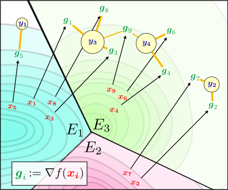
Figure 1: Points xisubscript𝑥𝑖x_{i} mapped onto points gi:=f(xi)assignsubscript𝑔𝑖𝑓subscript𝑥𝑖g_{i}:=\nabla f(x_{i}) for a function f𝑓f that is locally smooth strongly convex. SSNB potentials are such that the measure of endpoints gisubscript𝑔𝑖g_{i} is as close as possible (in W2subscript𝑊2W_{2} sense) to the measure supported on the yjsubscript𝑦𝑗y_{j}. Here this would be the sum of the squares of the length of these orange sticks.

Near-Brenier Smooth Strongly Convex Potentials. We will seek functions f𝑓f that are \ell-strongly convex and L𝐿L-smooth (or, alternatively, locally so) while at the same time such that fμsubscript𝑓𝜇\nabla f_{\sharp}\mu is as close as possible to the target ν𝜈\nu. If fμsubscript𝑓𝜇\nabla f_{\sharp}\mu were to be exactly equal to ν𝜈\nu, such a function would be called a Brenier potential. We quantify that nearness in terms of the Wasserstein distance between the push-foward of μ𝜇\mu and ν𝜈\nu to define:

Definition 1.

Let \mathcal{E} be a partition of dsuperscript𝑑\mathbb{R}^{d} and 0L0𝐿0\leq\ell\leq L. For μ,ν𝒫2(d)𝜇𝜈subscript𝒫2superscript𝑑\mu,\nu\in\mathscr{P}_{2}(\mathbb{R}^{d}), we call fsubscript𝑓{{f}_{\star}} a (\mathcal{E}-locally) L𝐿L-smooth \ell-strongly convex nearest Brenier (SSNB) potential between μ𝜇\mu and ν𝜈\nu if

fargminf,L,W2(fμ,ν).subscript𝑓subscriptargmin𝑓subscript𝐿subscript𝑊2subscript𝑓𝜇𝜈{{f}_{\star}}\in\operatorname*{arg\,min}_{f\in\mathcal{F}_{\ell,L,\mathcal{E}}}W_{2}\left(\nabla f_{\sharp}\mu,\nu\right).
Remark 1.

The existence of an SSNB potential is proved in the supplementary material. When ={d}superscript𝑑\mathcal{E}=\{\mathbb{R}^{d}\}, the gradient of any SSNB potential fsubscript𝑓{{f}_{\star}} defines an optimal transport map between μ𝜇\mu and fμsubscriptsubscript𝑓𝜇{\nabla{{f}_{\star}}}_{\sharp}\mu. The associated transport value W22(μ,fμ)superscriptsubscript𝑊22𝜇subscriptsubscript𝑓𝜇W_{2}^{2}\left(\mu,{\nabla{{f}_{\star}}}_{\sharp}\mu\right) does not define a metric between μ𝜇\mu and ν𝜈\nu because it is not symmetric, and W2(μ,fμ)=0⇏μ=νsubscript𝑊2𝜇subscriptsubscript𝑓𝜇0⇏𝜇𝜈W_{2}(\mu,{\nabla{{f}_{\star}}}_{\sharp}\mu)=0\not\Rightarrow\mu=\nu (take any ν𝜈\nu that is not a Dirac and μ=δ𝔼[ν]𝜇subscript𝛿𝔼𝜈\mu=\delta_{\operatorname{\mathbb{E}}[\nu]}). For more general partitions \mathcal{E} one only has that property locally, and fsubscript𝑓{{f}_{\star}} can therefore be interpreted as a piecewise convex potential, giving rise to piecewise optimal transport maps, as illustrated in Figure 1.

Algorithmic Formulation as an Alternate QCQP/Wasserstein Problem. We will work from now on with two discrete measures μ=i=1naiδxi𝜇superscriptsubscript𝑖1𝑛subscript𝑎𝑖subscript𝛿subscript𝑥𝑖\mu=\sum_{i=1}^{n}a_{i}\delta_{x_{i}} and ν=j=1mbjδyj𝜈superscriptsubscript𝑗1𝑚subscript𝑏𝑗subscript𝛿subscript𝑦𝑗\nu=\sum_{j=1}^{m}b_{j}\delta_{y_{j}}, with supports defined as x1,xndsubscript𝑥1subscript𝑥𝑛superscript𝑑x_{1},\ldots x_{n}\in\mathbb{R}^{d}, y1,ymdsubscript𝑦1subscript𝑦𝑚superscript𝑑y_{1},\ldots y_{m}\in\mathbb{R}^{d}, and 𝐚=(a1,,an)𝐚subscript𝑎1subscript𝑎𝑛\mathbf{a}=(a_{1},\dots,a_{n}) and 𝐛=(b1,,bm)𝐛subscript𝑏1subscript𝑏𝑚\mathbf{b}=(b_{1},\dots,b_{m}) are probability weight vectors. We write 𝒰(𝐚,𝐛)𝒰𝐚𝐛\mathcal{U}(\mathbf{a},\mathbf{b}) for the transportation polytope with marginals 𝐚𝐚\mathbf{a} and 𝐛𝐛\mathbf{b}, namely the set of n×m𝑛𝑚n\times m matrices with nonnegative entries such that their row-sum and column-sum are respectively equal to 𝐚𝐚\mathbf{a} and 𝐛𝐛\mathbf{b}. Set a desired smoothness L>0𝐿0L>0 and strong-convexity parameter L𝐿\ell\leq L, and choose a partition \mathcal{E} of dsuperscript𝑑\mathbb{R}^{d} (in our experiments \mathcal{E} is either {d}superscript𝑑\{\mathbb{R}^{d}\}, or computed using a K𝐾K-means partition of suppμsupp𝜇\operatorname{supp}{\mu}). For kKk\in\llbracket K\rrbracket, we write Ik={in s.t. xiEk}I_{k}=\left\{i\in\llbracket n\rrbracket\text{ s.t. }x_{i}\in E_{k}\right\}. The infinite dimensional optimization problem introduced in Definition 1 can be reduced to a QCQP that only focuses on the values and gradients of f𝑓f at the points xisubscript𝑥𝑖x_{i}. This result follows from the literature in the study of first order methods, which considers optimizing over the set of convex functions with prescribed smoothness and strong-convexity constants (see for instance (Taylor, 2017, Theorem 3.8 and Theorem 3.14)). We exploit such results to show that an SSNB f𝑓f can not only be estimated at those points xisubscript𝑥𝑖x_{i}, but also more generally recovered at any arbitrary point in dsuperscript𝑑\mathbb{R}^{d}.

Theorem 1.

The n𝑛n values ui:=f(xi)assignsubscript𝑢𝑖𝑓subscript𝑥𝑖u_{i}:=f(x_{i}), and gradients zi:=f(xi)assignsubscript𝑧𝑖𝑓subscript𝑥𝑖z_{i}:=\nabla f(x_{i}) of a SSNB potential f,L,𝑓subscript𝐿f\in\mathcal{F}_{\ell,L,\mathcal{E}} can be recovered as:

minz1,zndunW22(i=1naiδzi,ν):=minP𝒰(a,b)i,jPijziyj2assignsubscriptsubscript𝑧1subscript𝑧𝑛superscript𝑑𝑢superscript𝑛superscriptsubscript𝑊22superscriptsubscript𝑖1𝑛subscript𝑎𝑖subscript𝛿subscript𝑧𝑖𝜈subscript𝑃𝒰𝑎𝑏subscript𝑖𝑗subscript𝑃𝑖𝑗superscriptnormsubscript𝑧𝑖subscript𝑦𝑗2\displaystyle\min_{\begin{subarray}{c}z_{1},\ldots z_{n}\in\mathbb{R}^{d}\\ u\in\mathbb{R}^{n}\end{subarray}}W_{2}^{2}\left(\sum_{i=1}^{n}a_{i}\delta_{z_{i}},\nu\right):=\min_{P\in\mathcal{U}(a,b)}\sum_{i,j}P_{ij}\|z_{i}-y_{j}\|^{2} (1)
s.t. kK,i,jIk,formulae-sequences.t. for-all𝑘𝐾for-all𝑖𝑗subscript𝐼𝑘\displaystyle\textrm{s.t. }\forall k\leq K,\forall i,j\in I_{k},
uiuj+zj,xixjsubscript𝑢𝑖subscript𝑢𝑗subscript𝑧𝑗subscript𝑥𝑖subscript𝑥𝑗\displaystyle\qquad u_{i}\geq u_{j}+\langle z_{j},x_{i}-x_{j}\,\rangle
+12(1/L)(1Lzizj2+xixj2\displaystyle\qquad\qquad+\frac{1}{2(1-\ell/L)}\left(\frac{1}{L}\|z_{i}-z_{j}\|^{2}+\ell\|x_{i}-x_{j}\|^{2}\right.
2Lzjzi,xjxi).\displaystyle\qquad\qquad\qquad\qquad\qquad\left.-2\frac{\ell}{L}\langle z_{j}-z_{i},x_{j}-x_{i}\,\rangle\right).

Moreover, for xEk𝑥subscript𝐸𝑘x\in E_{k}, v:=f(x)assign𝑣𝑓𝑥v:=f(x) and g:=f(x)assign𝑔𝑓𝑥g:=\nabla f(x) can be recovered as:

minv,gdvsubscriptformulae-sequence𝑣𝑔superscript𝑑𝑣\displaystyle\min_{v\in\mathbb{R},\,g\in\mathbb{R}^{d}}v (2)
s.t.iIk,v ui+zi,xxi+12(1/L)(1Lgzi2+xxi22Lzig,xix).formulae-sequencestformulae-sequencefor-all𝑖subscript𝐼𝑘𝑣 subscript𝑢𝑖subscript𝑧𝑖𝑥subscript𝑥𝑖121𝐿1𝐿superscriptdelimited-∥∥𝑔subscript𝑧𝑖2superscriptdelimited-∥∥𝑥subscript𝑥𝑖22𝐿subscript𝑧𝑖𝑔subscript𝑥𝑖𝑥\displaystyle\begin{split}\mathrm{\quad s.t.}\,\forall i\in I_{k},v\geq&\text{ }u_{i}+\langle z_{i},x-x_{i}\,\rangle\\ &+\frac{1}{2(1-\ell/L)}\left(\frac{1}{L}\|g-z_{i}\|^{2}\right.\\ &\left.+\ell\|x-x_{i}\|^{2}-2\frac{\ell}{L}\langle z_{i}-g,x_{i}-x\,\rangle\right).\end{split}

We refer to the supplementary material for the proof.

We provide algorithms to compute a SSNB potential in dimension d2𝑑2d\geq 2 when μ,ν𝜇𝜈\mu,\nu are discrete measures. In order to solve Problem (1), we will alternate between minimizing over (z1,,zn,u)subscript𝑧1subscript𝑧𝑛𝑢(z_{1},\ldots,z_{n},u) and computing a coupling P𝑃P solving the OT problem. The OT computation can be efficiently carried out using Sinkhorn’s algorithm (Cuturi, 2013). The other minimization is a convex QCQP, separable in K𝐾K smaller convex QCQP that can be solved efficiently. We use the barycentric projection (see Definition 2 below) of μ𝜇\mu as an initialization for the points z𝑧z.

4 ONE-DIMENSIONAL CASE AND THE LINK WITH CONSTRAINED ISOTONIC REGRESSION

We consider first SSNB potentials in arguably the simplest case, namely that of distributions on the real line. We use the definition of the “barycentric projection” of a coupling (Ambrosio et al., 2006, Def.5.4.2), which is the most geometrically meaningful way to recover a map from a coupling.

Definition 2 (Barycentric Projection).

Let μ,ν𝒫2(d)𝜇𝜈subscript𝒫2superscript𝑑\mu,\nu\in\mathscr{P}_{2}(\mathbb{R}^{d}), and take π𝜋\pi an optimal transport plan between μ𝜇\mu and ν𝜈\nu. The barycentric projection of π𝜋\pi is defined as the map π¯:x𝔼(X,Y)π[Y|X=x]:¯𝜋maps-to𝑥subscript𝔼similar-to𝑋𝑌𝜋conditional𝑌𝑋𝑥\overline{\pi}:x\mapsto\operatorname{\mathbb{E}}_{(X,Y)\sim\pi}[Y|X=x].

Theorem 12.4.4 in (Ambrosio et al., 2006) shows that π¯¯𝜋\overline{\pi} is the gradient a convex function. It is then admissible for the SSNB optimization problem defined in Theorem 1 as soon as it verifies regularity (Lipschitzness) and curvature (strongly increasing). Although the barycentric projection map is not optimal in general, the following proposition shows that it is however optimal for univariate measures:

Proposition 1.

Let μ,ν𝒫2()𝜇𝜈subscript𝒫2\mu,\nu\in\mathscr{P}_{2}(\mathbb{R}) and 0L0𝐿0\leq\ell\leq L. Suppose μ1𝜇much-less-thansuperscript1\mu\operatorname{\ll}\mathscr{L}^{1}, or is purely atomic. Then the set of SSNB potentials between μ𝜇\mu and ν𝜈\nu is the set of solutions to

minf,L,fπ¯L2(μ)2subscript𝑓subscript𝐿subscriptsuperscriptnormsuperscript𝑓¯𝜋2superscript𝐿2𝜇\min_{f\in\mathcal{F}_{\ell,L,\mathcal{E}}}\|f^{\prime}-\overline{\pi}\|^{2}_{L^{2}(\mu)}

where π𝜋\pi is the unique optimal transport plan between μ𝜇\mu and ν𝜈\nu given by (Santambrogio, 2015, Theorem 2.9).
Refer to caption
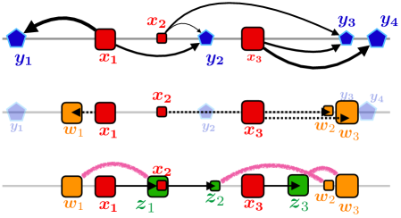
Figure 2: Top: optimal transport between two discrete measures μ,ν𝜇𝜈\mu,\nu. Middle: the barycentric projection 𝐰𝐰\mathbf{w} of points 𝐱𝐱\mathbf{x} is displayed and corresponds to a Monge map (no mass splitting). Considering here for instance =0.50.5\ell=0.5 and L=1𝐿1L=1, the map that associates xisubscript𝑥𝑖x_{i} to wisubscript𝑤𝑖w_{i} is not 111-Lipschitz at pairs (1,2)12(1,2) or (1,3)13(1,3) and over-contracting in pair (2,3)23(2,3). Bottom: To compute points zisubscript𝑧𝑖z_{i} that minimize their transport cost to the wisubscript𝑤𝑖w_{i} (pink curves) while still ensuring xizimaps-tosubscript𝑥𝑖subscript𝑧𝑖x_{i}\mapsto z_{i} is L𝐿L-Lipschitz and strongly increasing amounts to solving the L𝐿L-Lipschitz \ell-strongly increasing isotonic regression problem (3).

Discrete Computations. Suppose μ=i=1naiδxi𝜇superscriptsubscript𝑖1𝑛subscript𝑎𝑖subscript𝛿subscript𝑥𝑖\mu=\sum_{i=1}^{n}a_{i}\delta_{x_{i}} is discrete with x1xnsubscript𝑥1subscript𝑥𝑛x_{1}\leq\ldots\leq x_{n}, and ν𝜈\nu is arbitrary. Let us denote by Qνsubscript𝑄𝜈Q_{\nu} the (generalized) quantile function of ν𝜈\nu. Writing π𝜋\pi for the optimal transport plan between μ𝜇\mu and ν𝜈\nu, the barycentric projection π¯¯𝜋\overline{\pi} is explicit. Writing α0:=0assignsubscript𝛼00\alpha_{0}:=0, αi:=k=1iakassignsubscript𝛼𝑖superscriptsubscript𝑘1𝑖subscript𝑎𝑘\alpha_{i}:=\sum_{k=1}^{i}a_{k}, one has π¯(xi)=1aiαi1αiQν(t)𝑑t¯𝜋subscript𝑥𝑖1subscript𝑎𝑖superscriptsubscriptsubscript𝛼𝑖1subscript𝛼𝑖subscript𝑄𝜈𝑡differential-d𝑡\overline{\pi}(x_{i})=\frac{1}{a_{i}}\int_{\alpha_{i-1}}^{\alpha_{i}}Q_{\nu}(t)\,dt (proof in the supplementary material).

If ν𝜈\nu is also discrete, with weights 𝐛=(b1,,bm)𝐛subscript𝑏1subscript𝑏𝑚\mathbf{b}=(b_{1},\dots,b_{m}) and sorted support 𝐲=(y1,,ym)m𝐲subscript𝑦1subscript𝑦𝑚superscript𝑚\mathbf{y}=(y_{1},\dots,y_{m})\in\mathbb{R}^{m}, where y1ymsubscript𝑦1subscript𝑦𝑚y_{1}\leq\dots\leq y_{m}, one can recover the coordinates of the vector (π¯(xi))isubscript¯𝜋subscript𝑥𝑖𝑖(\overline{\pi}(x_{i}))_{i} of barycentric projections as

𝐰:=diag(𝐚1)𝐍𝐖(𝐚,𝐛)𝐲,assign𝐰diagsuperscript𝐚1𝐍𝐖𝐚𝐛𝐲\mathbf{w}:=\text{diag}(\mathbf{a}^{-1})\mathbf{NW}(\mathbf{a},\mathbf{b})\,\mathbf{y},

where 𝐍𝐖(𝐚,𝐛)𝐍𝐖𝐚𝐛\mathbf{NW}(\mathbf{a},\mathbf{b}) is the so-called North-west corner solution (Peyré & Cuturi, 2019, §3.4.2) obtained in linear time w.r.t n,m𝑛𝑚n,m by simply filling up greedily the transportation matrix from top-left to down-right. We deduce from Proposition 1 that a SSNB potential can be recovered by solving a weighted (and local, according to the partition \mathcal{E}) constrained isotonic regression problem (see Fig. 2):

minzni=1nai(ziwi)2subscript𝑧superscript𝑛superscriptsubscript𝑖1𝑛subscript𝑎𝑖superscriptsubscript𝑧𝑖subscript𝑤𝑖2\displaystyle\min_{z\in\mathbb{R}^{n}}\sum_{i=1}^{n}a_{i}(z_{i}-w_{i})^{2} (3)
s.t. kK,i,i+1Ik,formulae-sequences.t. for-all𝑘𝐾for-all𝑖𝑖1subscript𝐼𝑘\displaystyle\text{s.t. }\forall k\leq K,\,\forall i,i+1\in I_{k},
(xi+1xi)zi+1ziL(xi+1xi).subscript𝑥𝑖1subscript𝑥𝑖subscript𝑧𝑖1subscript𝑧𝑖𝐿subscript𝑥𝑖1subscript𝑥𝑖\displaystyle\qquad\quad\ell(x_{i+1}-x_{i})\leq z_{i+1}-z_{i}\leq L(x_{i+1}-x_{i}).

The gradient of a SSNB potential fsubscript𝑓{{f}_{\star}} can then be retrieved by taking an interpolation of xizimaps-tosubscript𝑥𝑖subscript𝑧𝑖x_{i}\mapsto z_{i} that is piecewise affine.

Algorithms solving the Lipschitz isotonic regression were first designed by Yeganova & Wilbur (2009) with a 𝒪(n2)𝒪superscript𝑛2\mathcal{O}(n^{2}) complexity. (Agarwal et al., 2010; Kakade et al., 2011) developed 𝒪(nlogn)𝒪𝑛𝑛\mathcal{O}(n\log{n}) algorithms. A Smooth NB potential can therefore be exactly computed in 𝒪(nlogn)𝒪𝑛𝑛\mathcal{O}(n\log{n}) time, which is the same complexity as of optimal transport in one dimension. Adding up the strongly increasing property, Problem (3) can also be seen as least-squares regression problem with box constraints. Indeed, introducing m𝑚m variables vi0subscript𝑣𝑖0v_{i}\geq 0, and defining zisubscript𝑧𝑖z_{i} as the partial sum 𝐯𝐯\mathbf{v}, namely zi=j=1ivjsubscript𝑧𝑖superscriptsubscript𝑗1𝑖subscript𝑣𝑗z_{i}=\sum_{j=1}^{i}v_{j} (or equivalently vi=zizi1subscript𝑣𝑖subscript𝑧𝑖subscript𝑧𝑖1v_{i}=z_{i}-z_{i-1} with z0:=0assignsubscript𝑧00z_{0}:=0), and writing ui=(xi+1xi)subscriptsuperscript𝑢𝑖subscript𝑥𝑖1subscript𝑥𝑖u^{-}_{i}=\ell(x_{i+1}-x_{i}), ui+=L(xi+1xi)subscriptsuperscript𝑢𝑖𝐿subscript𝑥𝑖1subscript𝑥𝑖u^{+}_{i}=L(x_{i+1}-x_{i}) one aims to find 𝐯𝐯\mathbf{v} that minimizes A𝐯𝐰a2superscriptsubscriptnorm𝐴𝐯𝐰𝑎2\|A\mathbf{v}-\mathbf{w}\|_{a}^{2} s.t. 𝐮𝐯𝐮+superscript𝐮𝐯superscript𝐮\mathbf{u^{-}}\leq\mathbf{v}\leq\mathbf{u^{+}}, where A𝐴A is the lower-triangular matrix of ones and a\|\cdot\|_{a} is the Euclidean norm weighted by a𝑎a. In our experiments, we have found that a projected gradient descent approach to solve this problem performed in practice as quickly as more specialized algorithms and was easier to parallelize when comparing a measure μ𝜇\mu to several measures ν𝜈\nu.

Refer to caption
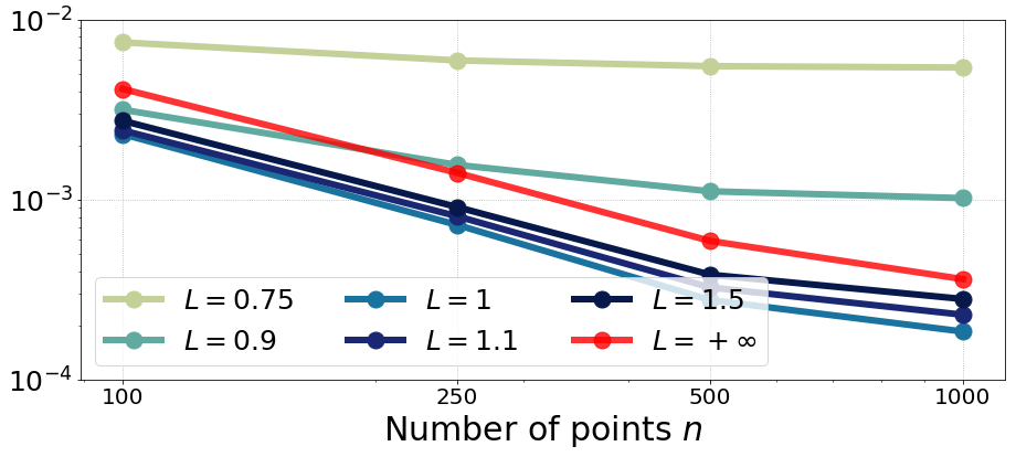
Figure 3: Take measures μ=ν𝜇𝜈\mu=\nu be the uniform measure over [0,1]01[0,1]. For several n𝑛n, we consider μ^n,ν^nsubscript^𝜇𝑛subscript^𝜈𝑛\hat{\mu}_{n},\hat{\nu}_{n} empirical measures over n𝑛n iid samples from μ,ν𝜇𝜈\mu,\nu, from which we compute a SSNB potential f^nsubscript^𝑓𝑛\hat{f}_{n} with different values L𝐿L, and =min{1,L}1𝐿\ell=\min\{1,L\} (and =00\ell=0 if L=𝐿L=\infty). We plot the estimation error |W22(μ^n,ζ^n)W22(μ,ν)|superscriptsubscript𝑊22subscript^𝜇𝑛subscript^𝜁𝑛superscriptsubscript𝑊22𝜇𝜈|W_{2}^{2}(\hat{\mu}_{n},\hat{\zeta}_{n})-W_{2}^{2}(\mu,\nu)| depending on n𝑛n and L𝐿L, averaged over 100100100 runs, where ζ^n=fn^μnsubscript^𝜁𝑛subscript^subscript𝑓𝑛subscript𝜇𝑛\hat{\zeta}_{n}=\hat{f_{n}}_{\sharp}\mu_{n}. If LLip(Id)=1𝐿LipId1L\leq\text{Lip}(\mathrm{Id})=1, the error does not converge to 00. Otherwise, the convergence is faster when L𝐿L is closer to 111. The case L=𝐿L=\infty corresponds to the classical OT estimator ζ^n=ν^nsubscript^𝜁𝑛subscript^𝜈𝑛\hat{\zeta}_{n}=\hat{\nu}_{n}.

5 ESTIMATION OF WASSERSTEIN DISTANCE AND MONGE MAP

Let μ,ν𝒫2(d)𝜇𝜈subscript𝒫2superscript𝑑\mu,\nu\in\mathscr{P}_{2}(\mathbb{R}^{d}) be two compactly supported measures with densities w.r.t the Lebesgue measure in dsuperscript𝑑\mathbb{R}^{d}. Brenier theorem gives the existence of an optimal Brenier potential fsubscript𝑓{{f}_{\star}}, i.e. fsubscript𝑓{{f}_{\star}} is convex and fμ=νsubscriptsubscript𝑓𝜇𝜈\nabla{{f}_{\star}}_{\sharp}\mu=\nu. Our goal is twofold: estimate the map fsubscript𝑓\nabla{{f}_{\star}} and the value of W2(μ,ν)subscript𝑊2𝜇𝜈W_{2}(\mu,\nu) from samples.

Let x1,,xnμsimilar-tosubscript𝑥1subscript𝑥𝑛𝜇x_{1},\ldots,x_{n}\sim\mu and y1,,ynνsimilar-tosubscript𝑦1subscript𝑦𝑛𝜈y_{1},\ldots,y_{n}\sim\nu be i.i.d samples from the measures, and define μ^n:=1ni=1nδxiassignsubscript^𝜇𝑛1𝑛superscriptsubscript𝑖1𝑛subscript𝛿subscript𝑥𝑖\hat{\mu}_{n}:=\frac{1}{n}\sum_{i=1}^{n}\delta_{x_{i}} and ν^n:=1ni=1nδyiassignsubscript^𝜈𝑛1𝑛superscriptsubscript𝑖1𝑛subscript𝛿subscript𝑦𝑖\hat{\nu}_{n}:=\frac{1}{n}\sum_{i=1}^{n}\delta_{y_{i}} the empirical measures over the samples.

Let f^nsubscript^𝑓𝑛\hat{f}_{n} be a SSNB potential between μ^nsubscript^𝜇𝑛\hat{\mu}_{n} and ν^nsubscript^𝜈𝑛\hat{\nu}_{n} with ={d}superscript𝑑\mathcal{E}=\{\mathbb{R}^{d}\}. Then for xsuppμ𝑥supp𝜇x\in\operatorname{supp}{\mu}, a natural estimator of f(x)subscript𝑓𝑥\nabla{{f}_{\star}}(x) is given by a solution f^n(x)subscript^𝑓𝑛𝑥\nabla\hat{f}_{n}(x) of (2). This defines an estimator f^n:dd:subscript^𝑓𝑛superscript𝑑superscript𝑑\nabla\hat{f}_{n}:\mathbb{R}^{d}\to\mathbb{R}^{d} of fsubscript𝑓\nabla{{f}_{\star}}, that we use to define a plug-in estimator for W2(μ,ν)subscript𝑊2𝜇𝜈W_{2}(\mu,\nu):

Definition 3.

We define the SSNB estimator of W22(μ,ν)superscriptsubscript𝑊22𝜇𝜈W_{2}^{2}(\mu,\nu) as W^22(μ,ν):=xf^n(x)2𝑑μ(x)assignsuperscriptsubscript^𝑊22𝜇𝜈superscriptnorm𝑥subscript^𝑓𝑛𝑥2differential-d𝜇𝑥\widehat{W}_{2}^{2}(\mu,\nu):=\int\|x-\nabla\hat{f}_{n}(x)\|^{2}\,d\mu(x).

Since f^nsubscript^𝑓𝑛\nabla\hat{f}_{n} is the gradient of a convex Brenier potential when ={d}superscript𝑑\mathcal{E}=\{\mathbb{R}^{d}\}, it is optimal between μ𝜇\mu and f^nμsubscriptsubscript^𝑓𝑛𝜇{\nabla\hat{f}_{n}}_{\sharp}\mu and W^2(μ,ν)=W2(μ,f^nμ)subscript^𝑊2𝜇𝜈subscript𝑊2𝜇subscriptsubscript^𝑓𝑛𝜇\widehat{W}_{2}(\mu,\nu)=W_{2}(\mu,{\nabla\hat{f}_{n}}_{\sharp}\mu). If {d}superscript𝑑\mathcal{E}\neq\{\mathbb{R}^{d}\}, f^nsubscript^𝑓𝑛\nabla\hat{f}_{n} is the gradient of a locally convex Brenier potential, and is not necessarily globally optimal between μ𝜇\mu and f^nμsubscriptsubscript^𝑓𝑛𝜇{\nabla\hat{f}_{n}}_{\sharp}\mu. In that case W^2(μ,ν)subscript^𝑊2𝜇𝜈\widehat{W}_{2}(\mu,\nu) is an approximate upper bound of W2(μ,f^nμ)subscript𝑊2𝜇subscriptsubscript^𝑓𝑛𝜇W_{2}(\mu,{\nabla\hat{f}_{n}}_{\sharp}\mu). In any case, the SSNB estimator can be computed using Monte-Carlo integration, whose estimation error does not depend on the dimension d𝑑d.

Algorithm 1 Monte-Carlo approximation of the SSNB estimator
  Input: μ^nsubscript^𝜇𝑛\hat{\mu}_{n}, ν^nsubscript^𝜈𝑛\hat{\nu}_{n}, partition \mathcal{E}, number N𝑁N of Monte-Carlo samples
  . (ui,zi)insubscriptsubscript𝑢𝑖subscript𝑧𝑖𝑖𝑛absent(u_{i},z_{i})_{i\leq n}\leftarrow solve SSNB (1) between μ^nsubscript^𝜇𝑛\hat{\mu}_{n}, ν^nsubscript^𝜈𝑛\hat{\nu}_{n}
  for jNj\in\llbracket N\rrbracket do
     . Draw x^jμsimilar-tosubscript^𝑥𝑗𝜇\hat{x}_{j}\sim\mu
     . Find k𝑘k s.t. x^jEksubscript^𝑥𝑗subscript𝐸𝑘\hat{x}_{j}\in E_{k} (k-means)
     . f^n(x^j)subscript^𝑓𝑛subscript^𝑥𝑗absent\nabla\hat{f}_{n}(\hat{x}_{j})\leftarrow solve QCQP (2)
  end for
  Output: W^=[(1/N)j=1Nx^jf^n(x^j)2]1/2^𝑊superscriptdelimited-[]1𝑁superscriptsubscript𝑗1𝑁superscriptnormsubscript^𝑥𝑗subscript^𝑓𝑛subscript^𝑥𝑗212\widehat{W}=\left[(1/N)\sum_{j=1}^{N}\|\hat{x}_{j}-\nabla\hat{f}_{n}(\hat{x}_{j})\|^{2}\right]^{1/2}

We show that when the Brenier potential fsubscript𝑓{{f}_{\star}} is globally regular, the SSNB estimator is strongly consistent:

Proposition 2.

Choose ={d}superscript𝑑\mathcal{E}=\{\mathbb{R}^{d}\}, 0L0𝐿0\leq\ell\leq L. If f,L,subscript𝑓subscript𝐿{{f}_{\star}}\in\mathcal{F}_{\ell,L,\mathcal{E}}, it almost surely holds:

|W2(μ,ν)W^2(μ,ν)|n0.subscript𝑊2𝜇𝜈subscript^𝑊2𝜇𝜈𝑛0\left|W_{2}(\mu,\nu)-\widehat{W}_{2}(\mu,\nu)\right|\underset{n\to\infty}{\longrightarrow}0.

The study of the theoretical rate of convergence of this estimator is beyond the scope of this work. Recent results (Hütter & Rigollet, 2019; Flamary et al., 2019) show that assuming some regularity of the Monge map fsubscript𝑓\nabla{{f}_{\star}} leads to improved sample complexity rates. Numerical simulations (see section 6.1) seem to indicate a reduced estimation error for SSNB over the classical W2(μ^n,ν^n)subscript𝑊2subscript^𝜇𝑛subscript^𝜈𝑛W_{2}(\hat{\mu}_{n},\hat{\nu}_{n}), even in the case where fsubscript𝑓\nabla{{f}_{\star}} is only locally Lipschitz and {d}superscript𝑑\mathcal{E}\neq\{\mathbb{R}^{d}\}. If L<Lip(f)𝐿Lipsubscript𝑓L<\text{Lip}(\nabla{{f}_{\star}}), the SSNB estimator W^2(μ,ν)subscript^𝑊2𝜇𝜈\widehat{W}_{2}(\mu,\nu) is not consistent, as can be seen in Figure 3.

6 EXPERIMENTS

All the computations were performed on a i9 2,9 GHz CPU, using MOSEK as a convex QCQP solver.

6.1 Numerical Estimation of Wasserstein Distances and Monge Maps

In this experiment, we consider two different settings:
Global regularity: μ𝜇\mu is the uniform measure over the unit cube in dsuperscript𝑑\mathbb{R}^{d}, and ν=Tμ𝜈subscript𝑇𝜇\nu=T_{\sharp}\mu where T(x)=Ωdx𝑇𝑥subscriptΩ𝑑𝑥T(x)=\Omega_{d}x, where ΩdsubscriptΩ𝑑\Omega_{d} is the diagonal matrix with diagonal coefficients: 0.8+0.4d1(i1)0.80.4𝑑1𝑖10.8+\frac{0.4}{d-1}(i-1), for idi\in\llbracket d\rrbracket. T𝑇T is the gradient of the convex function f:x12Ω1/2x2:𝑓maps-to𝑥12superscriptnormsuperscriptΩ12𝑥2f:x\mapsto\frac{1}{2}\|\Omega^{1/2}x\|^{2}, so it is the optimal transport map. f𝑓f is globally =0.80.8\ell=0.8-strongly convex and L=1.2𝐿1.2L=1.2-smooth.
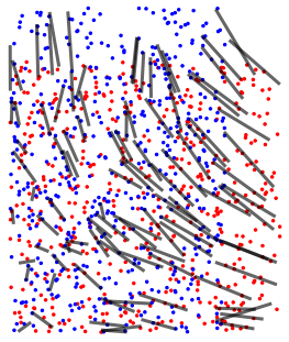
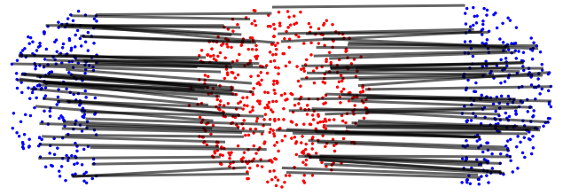
Local Regularity: μ𝜇\mu is the uniform measure over the unit ball in dsuperscript𝑑\mathbb{R}^{d}, and ν=Tμ𝜈subscript𝑇𝜇\nu=T_{\sharp}\mu where T(x1,,xd)=(x1+2sign(x1),x2,,xd)𝑇subscript𝑥1subscript𝑥𝑑subscript𝑥12signsubscript𝑥1subscript𝑥2subscript𝑥𝑑T(x_{1},\ldots,x_{d})=(x_{1}+2\operatorname{sign}(x_{1}),x_{2},\ldots,x_{d}). As can be seen in Figure 4 (bottom), T𝑇T splits the unit ball into two semi-balls. T𝑇T is a subgradient of the convex function f:x12x2+2|x1|:𝑓maps-to𝑥12superscriptnorm𝑥22subscript𝑥1f:x\mapsto\frac{1}{2}\|x\|^{2}+2|x_{1}|, so it is the optimal transport map. f𝑓f is =11\ell=1-strongly convex, but is not smooth: f𝑓\nabla f is not even continuous. However, f𝑓f is L=1𝐿1L=1-smooth by parts.

Refer to caption
Refer to caption
Figure 4: In the global (top) and local (bottom) regularity settings with d=2𝑑2d=2, we plot n=500𝑛500n=500 i.i.d samples from μ𝜇\mu (red) and ν𝜈\nu (blue). Black lines show the displacements xf^n(x)maps-to𝑥subscript^𝑓𝑛𝑥x\mapsto\nabla\hat{f}_{n}(x) for some new points xsupp(μ)supp(μ^n)𝑥supp𝜇suppsubscript^𝜇𝑛x\in\operatorname{supp}(\mu)\setminus\operatorname{supp}(\hat{\mu}_{n}), computed by solving QCQP (2).

For each of those two settings, we consider i.i.d samples x1,,xnμsimilar-tosubscript𝑥1subscript𝑥𝑛𝜇x_{1},\ldots,x_{n}\sim\mu and y1,,ynνsimilar-tosubscript𝑦1subscript𝑦𝑛𝜈y_{1},\ldots,y_{n}\sim\nu for different values of n𝑛n\in\mathbb{N}, and denote by μ^nsubscript^𝜇𝑛\hat{\mu}_{n} and ν^nsubscript^𝜈𝑛\hat{\nu}_{n} the respective empirical measures on these points. Given a number of clusters 1Kn1𝐾𝑛1\leq K\leq n, we compute the partition ={E1,,EK}subscript𝐸1subscript𝐸𝐾\mathcal{E}=\{E_{1},\ldots,E_{K}\} by running k-means with K𝐾K clusters on data x1,,xnsubscript𝑥1subscript𝑥𝑛x_{1},\ldots,x_{n}. In both settings, we run the algorithms with ^=0.6^0.6\hat{\ell}=0.6 and L^=1.4^𝐿1.4\hat{L}=1.4. We give experimental results on the statistical performance of our SSNB estimator, computed using Monte-Carlo integration, compared to the classical optimal transport estimator W2(μ^n,ν^n)subscript𝑊2subscript^𝜇𝑛subscript^𝜈𝑛W_{2}(\hat{\mu}_{n},\hat{\nu}_{n}). This performance depends on three parameters: the number n𝑛n of points, the dimension d𝑑d and the number of clusters K𝐾K.

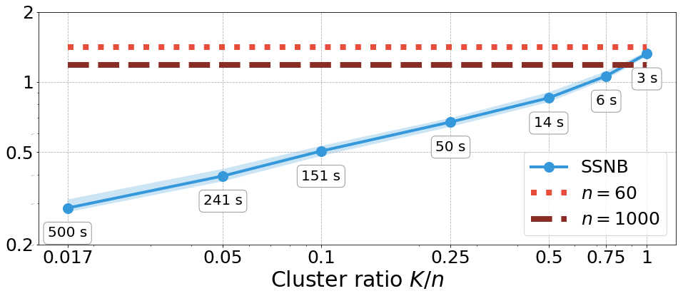
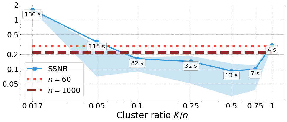
In Figure 5, we plot the estimation error depending on the cluster ratio K/n𝐾𝑛K/n for fixed n=60𝑛60n=60 and d=30𝑑30d=30. In the global regularity setting (Figure 5 top), the error seems to be exponentially increasing in K𝐾K, whereas the computation time decreases with K𝐾K: there is a trade-off between accuracy and computation time. In the local regularity setting (Figure 5 bottom), the estimation error is large when the number of clusters is too small (because we ask for too much regularity) or too large. Interestingly, the number of clusters can be taken large and still leads to good results. In both settings, even a large number of clusters is enough to outperform the classical OT estimator, even when SSNB is computed with a much smaller number of points. Note that when K/n=1𝐾𝑛1K/n=1, the SSNB estimator is basically equivalent (up to the Monte-Carlo integration error) to the classical OT estimator.
Refer to caption
Refer to caption
Figure 5: In the global (top) and local (bottom) regularity settings, we plot (on a log-log scale) the estimation error |W2(μ,ν)W^2(μ,ν)|subscript𝑊2𝜇𝜈subscript^𝑊2𝜇𝜈|W_{2}(\mu,\nu)-\widehat{W}_{2}(\mu,\nu)| (blue line) depending on the cluster ratio K/n𝐾𝑛K/n, with fixed number of points n=60𝑛60n=60, dimension d=30𝑑30d=30 and Monte-Carlo samples N=50𝑁50N=50. The curves/shaded areas show the mean error/25%-75% percentiles over 202020 data samples. The bubbles show the mean running time for the SSNB estimator computation. We plot the classical estimation error for n=60𝑛60n=60 (light red dotted) and n=1000𝑛1000n=1000 (dark red dashed) for comparison.

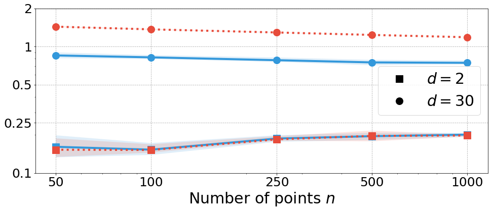
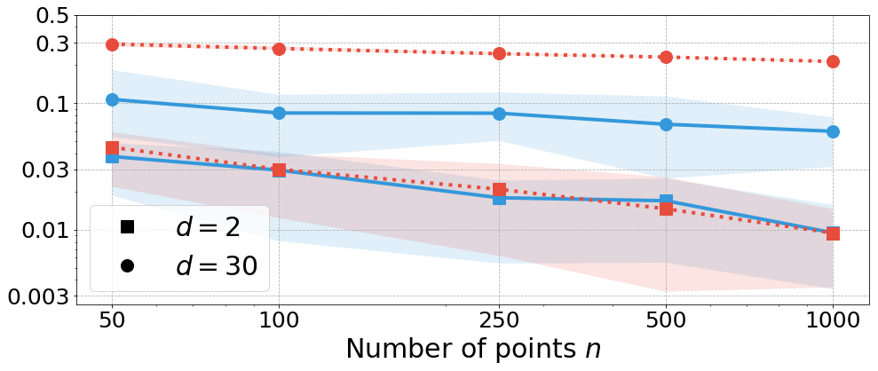
In Figure 6, we plot the estimation error depending on the number of points n𝑛n, for fixed cluster ratio K/n𝐾𝑛K/n and different dimension d{2,30}𝑑230d\in\{2,30\}. In both settings, and for both low (d=2𝑑2d=2) and high (d=30𝑑30d=30) dimension, the SSNB estimator seem to have the same rate as the classical OT estimator, but a much better constant in high dimension. This means that in high dimension, the SSNB estimator computed with a small number of points can be much more accurate that the classical OT estimator computed with a large number of points.
Refer to caption
Refer to caption
Figure 6: In the global (top) and local (bottom) regularity settings, we plot the estimation error of SSNB |W2(μ,ν)W^2(μ,ν)|subscript𝑊2𝜇𝜈subscript^𝑊2𝜇𝜈|W_{2}(\mu,\nu)-\widehat{W}_{2}(\mu,\nu)| (blue line) and classical OT estimator |W2(μ,ν)W2(μ^n,ν^n)|subscript𝑊2𝜇𝜈subscript𝑊2subscript^𝜇𝑛subscript^𝜈𝑛|W_{2}(\mu,\nu)-W_{2}(\hat{\mu}_{n},\hat{\nu}_{n})| (red dotted) depending on the number of points n{50,100,250,500,1000}𝑛501002505001000n\in\{50,100,250,500,1000\}, for dimension d{2,30}𝑑230d\in\{2,30\}. Here, the cluster ratios are taken constant equal to 0.50.50.5 (resp. 0.750.750.75) for the global (resp. local) regularity experiment. The number of Monte-Carlo samples is N=50𝑁50N=50. The curves/shaded areas show the mean error/25%-75% percentiles over 202020 data samples.

6.2 Domain Adaptation

Domain adaptation is a way to transfer knowledge from a source to a target dataset. The source dataset consists of labelled data, and the goal is to classify the target data. Courty et al. (2016); Perrot et al. (2016) proposed to use optimal transport (and different regularized version of OT) to perform such a task: the OT map from the source dataset to the target dataset (seen as empirical measures over the source/target data) is computed. Then each target data is labelled according to the label of its nearest neighbor among the transported source data.

The Caltech-Office datasets A, C, D, W contain images of ten different objects coming from four different sources: Amazon, Caltech-256, DSLR and Webcam. We consider DeCAF6 features (Donahue et al., 2014), which are sparse 409640964096-dimensional vectors. For each pair of source/target datasets, both datasets are cut in half (train and test): hyperparameters are learnt on the train half and we report the mean (±plus-or-minus\pm std) test accuracy over 10 random cuts, computed using a 111-Nearest Neighbour classifier on the transported source data. Results for OT, entropic OT, Group-Lasso and entropy regularized OT and SSNB are given in Table 1.

In order to compute the SSNB mapping, we a) quantize the source using k-means in each class with k=4𝑘4k=4 centroids, b) learn the SSNB map between the 404040 centroids and the target by solving (1), c) transport the source data by solving (2).

Domains OT OT-IT OT-GL SSNB
A bold-→\boldsymbol{\rightarrow} C 74.074.074.0 81.0±2.2plus-or-minus81.02.281.0\pm 2.2 86.6±1.0plus-or-minus86.61.0\boldsymbol{86.6\pm 1.0} 83.9±1.6plus-or-minus83.91.683.9\pm 1.6
A bold-→\boldsymbol{\rightarrow} D 65.065.065.0 84.3±5.2plus-or-minus84.35.2\boldsymbol{84.3\pm 5.2} 82.9±5.2plus-or-minus82.95.2\boldsymbol{82.9\pm 5.2} 79.2±3.7plus-or-minus79.23.7\boldsymbol{79.2\pm 3.7}
A bold-→\boldsymbol{\rightarrow} W 65.065.065.0 79.3±5.3plus-or-minus79.35.3\boldsymbol{79.3\pm 5.3} 81.6±3.1plus-or-minus81.63.1\boldsymbol{81.6\pm 3.1} 82.3±3.1plus-or-minus82.33.1\boldsymbol{82.3\pm 3.1}
C bold-→\boldsymbol{\rightarrow} A 75.375.375.3 90.3±1.3plus-or-minus90.31.390.3\pm 1.3 91.1±1.8plus-or-minus91.11.8\boldsymbol{91.1\pm 1.8} 91.9±1.1plus-or-minus91.91.1\boldsymbol{91.9\pm 1.1}
C bold-→\boldsymbol{\rightarrow} D 65.665.665.6 83.9±4.0plus-or-minus83.94.0\boldsymbol{83.9\pm 4.0} 85.8±2.3plus-or-minus85.82.3\boldsymbol{85.8\pm 2.3} 81.1±4.9plus-or-minus81.14.981.1\pm 4.9
C bold-→\boldsymbol{\rightarrow} W 64.864.864.8 77.1±3.9plus-or-minus77.13.9\boldsymbol{77.1\pm 3.9} 81.9±5.1plus-or-minus81.95.1\boldsymbol{81.9\pm 5.1} 79.3±2.8plus-or-minus79.32.8\boldsymbol{79.3\pm 2.8}
D bold-→\boldsymbol{\rightarrow} A 69.669.669.6 88.3±3.1plus-or-minus88.33.188.3\pm 3.1 90.5±1.9plus-or-minus90.51.9\boldsymbol{90.5\pm 1.9} 91.2±0.8plus-or-minus91.20.8\boldsymbol{91.2\pm 0.8}
D bold-→\boldsymbol{\rightarrow} C 66.466.466.4 78.0±2.9plus-or-minus78.02.978.0\pm 2.9 85.6±2.2plus-or-minus85.62.2\boldsymbol{85.6\pm 2.2} 81.4±1.9plus-or-minus81.41.981.4\pm 1.9
D bold-→\boldsymbol{\rightarrow} W 84.784.784.7 96.1±2.1plus-or-minus96.12.1\boldsymbol{96.1\pm 2.1} 93.8±2.1plus-or-minus93.82.193.8\pm 2.1 95.6±1.5plus-or-minus95.61.5\boldsymbol{95.6\pm 1.5}
W bold-→\boldsymbol{\rightarrow} A 66.466.466.4 82.5±4.3plus-or-minus82.54.382.5\pm 4.3 89.3±2.7plus-or-minus89.32.7\boldsymbol{89.3\pm 2.7} 89.8±2.9plus-or-minus89.82.9\boldsymbol{89.8\pm 2.9}
W bold-→\boldsymbol{\rightarrow} C 62.562.562.5 74.8±2.3plus-or-minus74.82.374.8\pm 2.3 80.2±2.4plus-or-minus80.22.480.2\pm 2.4 82.7±1.4plus-or-minus82.71.4\boldsymbol{82.7\pm 1.4}
W bold-→\boldsymbol{\rightarrow} D 87.387.387.3 97.5±2.1plus-or-minus97.52.1\boldsymbol{97.5\pm 2.1} 96.4±3.7plus-or-minus96.43.7\boldsymbol{96.4\pm 3.7} 95.9±3.2plus-or-minus95.93.2\boldsymbol{95.9\pm 3.2}
\hdashlineMean 70.6±7.8plus-or-minus70.67.870.6\pm 7.8 84.4±7.0plus-or-minus84.47.0\boldsymbol{84.4\pm 7.0} 87.1±4.9plus-or-minus87.14.9\boldsymbol{87.1\pm 4.9} 86.2±6.0plus-or-minus86.26.0\boldsymbol{86.2\pm 6.0}
Table 1: OT-IT: Entropy regularized OT. OT-GL: Entropy + Group Lasso regularized OT. Search intervals for OT-IT and OT-GL are ϵ,η{103,,103}italic-ϵ𝜂superscript103superscript103\epsilon,\eta\in\{10^{-3},\ldots,10^{3}\} with normalized cost, and for SSNB: {0.2,0.5,0.7,0.9}0.20.50.70.9\ell\in\{0.2,0.5,0.7,0.9\}, L{0.3,0.5,0.7,0.9,1.3}𝐿0.30.50.70.91.3L\in\{0.3,0.5,0.7,0.9,1.3\}. The best results are in bold.

6.3 Color Transfer

Given a source and a target image, the goal of color transfer is to transform the colors of the source image so that it looks similar to the target image color palette. Optimal transport has been used to carry out such a task, see e.g. (Bonneel et al., 2015; Ferradans et al., 2014; Rabin et al., 2014). Each image is represented by a point cloud in the RGB color space identified with [0,1]3superscript013[0,1]^{3}. The optimal transport plan π𝜋\pi between the two point clouds give, up to a barycentric projection, a transfer color mapping.

It is natural to ask that similar colors are transferred to similar colors, and that different colors are transferred to different colors. These two demands translate into the smoothness and strong convexity of the Brenier potential from which derives the color transfer mapping. We therefore propose to compute a SSNB potential and map between the source and target distributions in the color space.

In order to make the computations tractable, we compute a k-means clustering with 303030 clusters for each point cloud, and compute the SSNB potential using the two empirical measures on the centroids.

We then recompute a k-means clustering of the source point cloud with 100010001000 clusters. For each of the 100010001000 centroids, we compute its new color by solving QCQP (2). A pixel in the original image then sees its color changed according to the transformation of its nearest neighbor among the 100010001000 centroids.

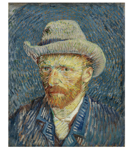
In Figure 7, we show the color-transferred results using OT, or SSNB potentials for different values of parameters \ell and L𝐿L. Smaller values of L𝐿L give more uniform colors, while larger values of \ell give more contrast.

Refer to caption
(a) Original     Image
Refer to caption
(b) Target Image Classical OT, W0𝑊0W\approx 0
Refer to caption
(c) Classical OT, W0𝑊0W\approx 0
Refer to caption
(d) =0,L=1formulae-sequence0𝐿1\ell=0,L=1, W1×102𝑊1superscript102W\approx 1\times 10^{-2}
Refer to caption
(e) =.5,L=1formulae-sequence.5𝐿1\ell=.5,L=1, W1×102𝑊1superscript102W\approx 1\times 10^{-2}
Refer to caption
(f) =1,L=1formulae-sequence1𝐿1\ell=1,L=1, W2×102𝑊2superscript102W\approx 2\times 10^{-2}
Refer to caption
(g) =0,L=2formulae-sequence0𝐿2\ell=0,L=2, W4×103𝑊4superscript103W\approx 4\times 10^{-3}
Refer to caption
(h) =.5,L=2formulae-sequence.5𝐿2\ell=.5,L=2, W5×103𝑊5superscript103W\approx 5\times 10^{-3}
Refer to caption
(i) =1,L=2formulae-sequence1𝐿2\ell=1,L=2, W2×102𝑊2superscript102W\approx 2\times 10^{-2}
Refer to caption
(j) =0,L=5formulae-sequence0𝐿5\ell=0,L=5, W2×104𝑊2superscript104W\approx 2\times 10^{-4}
Refer to caption
(k) =.5,L=5formulae-sequence.5𝐿5\ell=.5,L=5, W1×103𝑊1superscript103W\approx 1\times 10^{-3}
Refer to caption
(l) =1,L=5formulae-sequence1𝐿5\ell=1,L=5, W2×102𝑊2superscript102W\approx 2\times 10^{-2}
Figure 7: (a) Schiele’s portrait. (b) Van Gogh’s portrait. (c) Color transfer using classical OT. (d)-(l) Color transfer using SSNB map, for {0,0.5,1}00.51\ell\in\{0,0.5,1\} and L{1,2,5}𝐿125L\in\{1,2,5\}. The value W𝑊W corresponds to the Wasserstein distance between the color distribution of the image and the color distribution of Van Gogh’s portrait. The smaller W𝑊W, the greater the fidelity to Van Gogh’s portrait colors.

7 CONCLUSION

We have proposed in this work the first computational procedure to estimate optimal transport that incorporates smoothness and strongly convex (local) constraints on the Brenier potential, or, equivalently, that ensures that the optimal transport map has (local) distortion that is both upper and lower bounded. These assumptions are natural for several problems, both high and low dimensional, can be implemented practically and advance the current knowledge on handling the curse of dimensionality in optimal transport.

Acknowledgments. We thank J. Altschuler for his remark that the QCQP (1) considered in Theorem 1 is in fact convex (unlike in the optimization literature where it is not) and can therefore be exactly solved and not approximated through an SDP.
F.P.P and M.C. acknowledge the support of a "Chaire d’excellence de l’IDEX Paris Saclay". A.A. is at the département d’informatique de l’ENS, École normale supérieure, UMR CNRS 8548, PSL Research University, 75005 Paris, France, and INRIA Sierra project-team. AA would like to acknowledge support from the ML and Optimisation joint research initiative with the fonds AXA pour la recherche and Kamet Ventures, a Google focused award, as well as funding by the French government under management of Agence Nationale de la Recherche as part of the "Investissements d’avenir" program, reference ANR-19-P3IA-0001 (PRAIRIE 3IA Institute).

References

  • Abadeh et al. (2015) Abadeh, S. S., Esfahani, P. M. M., and Kuhn, D. Distributionally robust logistic regression. In Advances in Neural Information Processing Systems, pp. 1576–1584, 2015.
  • Agarwal et al. (2010) Agarwal, P. K., Phillips, J. M., and Sadri, B. Lipschitz unimodal and isotonic regression on paths and trees. In Latin American Symposium on Theoretical Informatics, pp. 384–396. Springer, 2010.
  • Alaux et al. (2019) Alaux, J., Grave, E., Cuturi, M., and Joulin, A. Unsupervised hyper-alignment for multilingual word embeddings. In International Conference on Learning Representations, 2019.
  • Alt & Guibas (2000) Alt, H. and Guibas, L. J. Discrete geometric shapes: Matching, interpolation, and approximation. In Handbook of computational geometry, pp.  121–153. Elsevier, 2000.
  • Ambrosio et al. (2006) Ambrosio, L., Gigli, N., and Savaré, G. Gradient Flows in Metric Spaces and in the Space of Probability Measures. Springer, 2006.
  • Arjovsky et al. (2017) Arjovsky, M., Chintala, S., and Bottou, L. Wasserstein generative adversarial networks. Proceedings of the 34th International Conference on Machine Learning, 70:214–223, 2017.
  • Bonneel et al. (2015) Bonneel, N., Rabin, J., Peyré, G., and Pfister, H. Sliced and radon wasserstein barycenters of measures. Journal of Mathematical Imaging and Vision, 51(1):22–45, 2015.
  • Bonneel et al. (2016) Bonneel, N., Peyré, G., and Cuturi, M. Wasserstein barycentric coordinates: histogram regression using optimal transport. ACM Transactions on Graphics, 35(4):71:1–71:10, 2016.
  • Brenier (1987) Brenier, Y. Décomposition polaire et réarrangement monotone des champs de vecteurs. C. R. Acad. Sci. Paris Sér. I Math., 305(19):805–808, 1987.
  • Caffarelli (2000) Caffarelli, L. A. Monotonicity properties of optimal transportation and the fkg and related inequalities. Communications in Mathematical Physics, 214(3):547–563, 2000.
  • Caffarelli et al. (1999) Caffarelli, L. A., Kochengin, S. A., and Oliker, V. I. Problem of reflector design with given far-field scattering data. In Monge Ampère equation: applications to geometry and optimization, volume 226, pp.  13, 1999.
  • Cohen & Guibas (1999) Cohen, S. and Guibas, L. The earth mover’s distance under transformation sets. In Proceedings of the Seventh IEEE International Conference on Computer vision, volume 2, pp.  1076–1083. IEEE, 1999.
  • Courty et al. (2016) Courty, N., Flamary, R., Tuia, D., and Rakotomamonjy, A. Optimal transport for domain adaptation. IEEE transactions on pattern analysis and machine intelligence, 39(9):1853–1865, 2016.
  • Cuturi (2013) Cuturi, M. Sinkhorn distances: lightspeed computation of optimal transport. In Advances in Neural Information Processing Systems 26, pp. 2292–2300, 2013.
  • Cuturi & Peyré (2016) Cuturi, M. and Peyré, G. A smoothed dual approach for variational Wasserstein problems. SIAM Journal on Imaging Sciences, 9(1):320–343, 2016.
  • Donahue et al. (2014) Donahue, J., Jia, Y., Vinyals, O., Hoffman, J., Zhang, N., Tzeng, E., and Darrell, T. Decaf: A deep convolutional activation feature for generic visual recognition. In International conference on machine learning, pp. 647–655, 2014.
  • Drori & Teboulle (2014) Drori, Y. and Teboulle, M. Performance of first-order methods for smooth convex minimization: a novel approach. Mathematical Programming, 145(1-2):451–482, 2014.
  • Dudley (1969) Dudley, R. M. The speed of mean Glivenko-Cantelli convergence. Annals of Mathematical Statistics, 40(1):40–50, 1969.
  • Ferradans et al. (2014) Ferradans, S., Papadakis, N., Peyré, G., and Aujol, J.-F. Regularized discrete optimal transport. SIAM Journal on Imaging Sciences, 7(3):1853–1882, 2014.
  • Figalli (2010) Figalli, A. The optimal partial transport problem. Archive for Rational Mechanics and Analysis, 195(2):533–560, 2010.
  • Figalli (2017) Figalli, A. The Monge–Ampère equation and its applications. 2017.
  • Flamary et al. (2014) Flamary, R., Courty, N., Rakotomamonjy, A., and Tuia, D. Optimal transport with laplacian regularization. In NIPS 2014, Workshop on Optimal Transport and Machine Learning, 2014.
  • Flamary et al. (2019) Flamary, R., Lounici, K., and Ferrari, A. Concentration bounds for linear monge mapping estimation and optimal transport domain adaptation. arXiv preprint arXiv:1905.10155, 2019.
  • Frogner et al. (2015) Frogner, C., Zhang, C., Mobahi, H., Araya, M., and Poggio, T. A. Learning with a Wasserstein loss. In Advances in Neural Information Processing Systems, pp. 2053–2061, 2015.
  • Grave et al. (2019) Grave, E., Joulin, A., and Berthet, Q. Unsupervised alignment of embeddings with wasserstein procrustes. 2019.
  • Hashimoto et al. (2016) Hashimoto, T., Gifford, D., and Jaakkola, T. Learning population-level diffusions with generative RNNs. In International Conference on Machine Learning, pp. 2417–2426, 2016.
  • Hütter & Rigollet (2019) Hütter, J.-C. and Rigollet, P. Minimax rates of estimation for smooth optimal transport maps. arXiv preprint arXiv:1905.05828, 2019.
  • Kakade et al. (2011) Kakade, S. M., Kanade, V., Shamir, O., and Kalai, A. Efficient learning of generalized linear and single index models with isotonic regression. In Advances in Neural Information Processing Systems, pp. 927–935, 2011.
  • Mémoli (2011) Mémoli, F. Gromov–Wasserstein distances and the metric approach to object matching. Foundations of Computational Mathematics, 11(4):417–487, 2011.
  • Monge (1781) Monge, G. Mémoire sur la théorie des déblais et des remblais. Histoire de l’Académie Royale des Sciences, pp. 666–704, 1781.
  • Panaretos & Zemel (2019) Panaretos, V. M. and Zemel, Y. Statistical aspects of wasserstein distances. Annual Review of Statistics and Its Application, 6(1):405–431, 2019.
  • Perrot et al. (2016) Perrot, M., Courty, N., Flamary, R., and Habrard, A. Mapping estimation for discrete optimal transport. In Lee, D. D., Sugiyama, M., Luxburg, U. V., Guyon, I., and Garnett, R. (eds.), Advances in Neural Information Processing Systems 29, pp. 4197–4205. Curran Associates, Inc., 2016.
  • Peyré & Cuturi (2019) Peyré, G. and Cuturi, M. Computational optimal transport. Foundations and Trends in Machine Learning, 11(5-6):355–607, 2019. ISSN 1935-8237. doi: 10.1561/2200000073.
  • Rabin & Papadakis (2015) Rabin, J. and Papadakis, N. Convex color image segmentation with optimal transport distances. In International Conference on Scale Space and Variational Methods in Computer Vision, pp.  256–269. Springer, 2015.
  • Rabin et al. (2014) Rabin, J., Ferradans, S., and Papadakis, N. Adaptive color transfer with relaxed optimal transport. In 2014 IEEE International Conference on Image Processing (ICIP), pp.  4852–4856. IEEE, 2014.
  • Salimans et al. (2018) Salimans, T., Zhang, H., Radford, A., and Metaxas, D. Improving GANs using optimal transport. In International Conference on Learning Representations, 2018. URL https://openreview.net/forum?id=rkQkBnJAb.
  • Santambrogio (2015) Santambrogio, F. Optimal transport for applied mathematicians. Birkhauser, 2015.
  • Schiebinger et al. (2019) Schiebinger, G., Shu, J., Tabaka, M., Cleary, B., Subramanian, V., Solomon, A., Gould, J., Liu, S., Lin, S., Berube, P., et al. Optimal-transport analysis of single-cell gene expression identifies developmental trajectories in reprogramming. Cell, 176(4):928–943, 2019.
  • Solomon et al. (2015) Solomon, J., De Goes, F., Peyré, G., Cuturi, M., Butscher, A., Nguyen, A., Du, T., and Guibas, L. Convolutional Wasserstein distances: efficient optimal transportation on geometric domains. ACM Transactions on Graphics, 34(4):66:1–66:11, 2015.
  • Taylor (2017) Taylor, A. B. Convex interpolation and performance estimation of first-order methods for convex optimization. PhD thesis, 2017.
  • Taylor et al. (2017) Taylor, A. B., Hendrickx, J. M., and Glineur, F. Smooth strongly convex interpolation and exact worst-case performance of first-order methods. Mathematical Programming, 161(1-2):307–345, 2017.
  • Villani (2003) Villani, C. Topics in Optimal Transportation. Graduate Studies in Mathematics Series. American Mathematical Society, 2003. ISBN 9780821833124.
  • Villani (2009) Villani, C. Optimal Transport: Old and New, volume 338. Springer Verlag, 2009.
  • Yeganova & Wilbur (2009) Yeganova, L. and Wilbur, W. Isotonic regression under lipschitz constraint. Journal of optimization theory and applications, 141(2):429–443, 2009.

Appendix A PROOFS

Proof for Definition 1

We write a proof in the case where ={d}superscript𝑑\mathcal{E}=\{\mathbb{R}^{d}\}. If K>1𝐾1K>1, the proof can be applied independently on each set of the partition.

Let (fn)nsubscriptsubscript𝑓𝑛𝑛(f_{n})_{n\in\mathbb{N}} be such that fn(0)=0subscript𝑓𝑛00f_{n}(0)=0 for all n𝑛n\in\mathbb{N} and

W2[(fn)μ,ν]1n+1+inff,LW2[(f)μ,ν].subscript𝑊2subscriptsubscript𝑓𝑛𝜇𝜈1𝑛1subscriptinfimum𝑓subscript𝐿subscript𝑊2subscript𝑓𝜇𝜈W_{2}\left[(\nabla f_{n})_{\sharp}\mu,\nu\right]\leq\frac{1}{n+1}+\inf_{f\in\mathcal{F}_{\ell,L}}W_{2}\left[(\nabla f)_{\sharp}\mu,\nu\right].

Let x0supp(μ)subscript𝑥0supp𝜇x_{0}\in\operatorname{supp}(\mu). Then there exists C>0𝐶0C>0 such that for all n𝑛n\in\mathbb{N}, fn(x0)Cnormsubscript𝑓𝑛subscript𝑥0𝐶\|\nabla f_{n}(x_{0})\|\leq C. Indeed, suppose this is not true. Take r>0𝑟0r>0 such that V:=μ[B(x0,r)]>0assign𝑉𝜇delimited-[]𝐵subscript𝑥0𝑟0V:=\mu[B(x_{0},r)]>0. By Prokhorov theorem, there exists R>0𝑅0R>0 such that ν[B(0,R)]1V2𝜈delimited-[]𝐵0𝑅1𝑉2\nu\left[B(0,R)\right]\geq 1-\frac{V}{2}. Then for C>0𝐶0C>0 large enough, there exists an n𝑛n\in\mathbb{N} such that:

W22[(fn)μ,ν]=minπΠ(μ,ν)fn(x)y2𝑑π(x,y)fn(x)projB(0,R)[fn(x)]2𝑑μ(x)B(x0,r)supp(μ)fnprojB(0,R)[fn]2𝑑μ12VminxB(x0,r)yB(0,R)fn(x)y212V(CLrR)superscriptsubscript𝑊22subscriptsubscript𝑓𝑛𝜇𝜈subscript𝜋Π𝜇𝜈superscriptdelimited-∥∥subscript𝑓𝑛𝑥𝑦2differential-d𝜋𝑥𝑦superscriptdelimited-∥∥subscript𝑓𝑛𝑥subscriptproj𝐵0𝑅subscript𝑓𝑛𝑥2differential-d𝜇𝑥subscript𝐵subscript𝑥0𝑟supp𝜇superscriptdelimited-∥∥subscript𝑓𝑛subscriptproj𝐵0𝑅subscript𝑓𝑛2differential-d𝜇12𝑉subscript𝑥𝐵subscript𝑥0𝑟𝑦𝐵0𝑅superscriptdelimited-∥∥subscript𝑓𝑛𝑥𝑦212𝑉𝐶𝐿𝑟𝑅\begin{split}W_{2}^{2}&[(\nabla f_{n})_{\sharp}\mu,\nu]=\displaystyle\min_{\pi\in\Pi(\mu,\nu)}\int\|\nabla f_{n}(x)-y\|^{2}\,d\pi(x,y)\\ &\geq\displaystyle\int\|\nabla f_{n}(x)-\operatorname{proj}_{B(0,R)}\left[\nabla f_{n}(x)\right]\|^{2}\,d\mu(x)\\ &\geq\displaystyle\int_{B(x_{0},r)\cap\operatorname{supp}(\mu)}\|\nabla f_{n}-\operatorname{proj}_{B(0,R)}\left[\nabla f_{n}\right]\|^{2}\,d\mu\\ &\geq\frac{1}{2}V\displaystyle\min_{\begin{subarray}{c}x\in B(x_{0},r)\\ y\in B(0,R)\end{subarray}}\|\nabla f_{n}(x)-y\|^{2}\\ &\geq\frac{1}{2}V(C-Lr-R)\end{split}

which contradicts the definition of fnsubscript𝑓𝑛f_{n} when C𝐶C is sufficiently large.
Then for xd𝑥superscript𝑑x\in\mathbb{R}^{d},

fn(x)Lxx0+fn(x0)Lxx0+C.normsubscript𝑓𝑛𝑥𝐿norm𝑥subscript𝑥0normsubscript𝑓𝑛subscript𝑥0𝐿norm𝑥subscript𝑥0𝐶\|\nabla f_{n}(x)\|\leq L\|x-x_{0}\|+\|\nabla f_{n}(x_{0})\|\leq L\|x-x_{0}\|+C.

Since (fn)nsubscriptsubscript𝑓𝑛𝑛(\nabla f_{n})_{n\in\mathbb{N}} is equi-Lipschitz, it converges uniformly (up to a subsequence) to some function g𝑔g by Arzelà–Ascoli theorem. Note that g𝑔g is L𝐿L-Lipschitz.
Let ϵ>0italic-ϵ0\epsilon>0 and let N𝑁N\in\mathbb{N} such that nNfngϵ𝑛𝑁subscriptnormsubscript𝑓𝑛𝑔italic-ϵn\geq N\Rightarrow\|\nabla f_{n}-g\|_{\infty}\leq\epsilon. Then for nN𝑛𝑁n\geq N and xd𝑥superscript𝑑x\in\mathbb{R}^{d},

|fn(x)|=|01fn(tx),x𝑑t|x(g+ϵ)subscript𝑓𝑛𝑥superscriptsubscript01subscript𝑓𝑛𝑡𝑥𝑥differential-d𝑡norm𝑥subscriptnorm𝑔italic-ϵ|f_{n}(x)|=\bigg{|}\int_{0}^{1}\langle\nabla f_{n}(tx),x\,\rangle\,dt\bigg{|}\leq\|x\|(\|g\|_{\infty}+\epsilon)

so that (fn(x))subscript𝑓𝑛𝑥(f_{n}(x)) converges up to a subsequence. Let ϕ,ψitalic-ϕ𝜓\phi,\psi be two extractions and α,β𝛼𝛽\alpha,\beta such that fϕ(n)(x)αsubscript𝑓italic-ϕ𝑛𝑥𝛼f_{\phi(n)}(x)\to\alpha and fψ(n)(x)βsubscript𝑓𝜓𝑛𝑥𝛽f_{\psi(n)}(x)\to\beta. Then

|αβ|=limn|01fϕ(n)(tx)fψ(n)(tx),x𝑑t|limnxfϕ(n)fψ(n)=0.𝛼𝛽subscript𝑛superscriptsubscript01subscript𝑓italic-ϕ𝑛𝑡𝑥subscript𝑓𝜓𝑛𝑡𝑥𝑥differential-d𝑡subscript𝑛delimited-∥∥𝑥subscriptdelimited-∥∥subscript𝑓italic-ϕ𝑛subscript𝑓𝜓𝑛0\begin{split}|\alpha-\beta|&=\lim_{n\to\infty}\bigg{|}\int_{0}^{1}\langle\nabla f_{\phi(n)}(tx)-\nabla f_{\psi(n)}(tx),x\,\rangle\,dt\bigg{|}\\ &\leq\lim_{n\to\infty}\|x\|\|\nabla f_{\phi(n)}-\nabla f_{\psi(n)}\|_{\infty}=0.\end{split}

This shows that (fn)nNsubscriptsubscript𝑓𝑛𝑛𝑁(f_{n})_{n\in N} converges pointwise to some function fsubscript𝑓{{f}_{\star}}. In particular, fsubscript𝑓{{f}_{\star}} is convex. For xd𝑥superscript𝑑x\in\mathbb{R}^{d}, using Lebesgue’s dominated convergence theorem,

f(x)=limnfn(x)=limn01fn(tx),x𝑑t=01limnfn(tx),x𝑑t=01g(tx),x𝑑tsubscript𝑓𝑥subscript𝑛subscript𝑓𝑛𝑥subscript𝑛superscriptsubscript01subscript𝑓𝑛𝑡𝑥𝑥differential-d𝑡superscriptsubscript01subscript𝑛subscript𝑓𝑛𝑡𝑥𝑥differential-d𝑡superscriptsubscript01𝑔𝑡𝑥𝑥differential-d𝑡\begin{split}{{f}_{\star}}(x)&=\lim_{n\to\infty}f_{n}(x)=\lim_{n\to\infty}\int_{0}^{1}\langle\nabla f_{n}(tx),x\,\rangle\,dt\\ &=\int_{0}^{1}\left\langle\lim_{n\to\infty}\nabla f_{n}(tx),x\right\rangle\,dt=\int_{0}^{1}\langle g(tx),x\,\rangle\,dt\end{split}

so fsubscript𝑓{{f}_{\star}} is differentiable and f=gsubscript𝑓𝑔\nabla{{f}_{\star}}=g. Using Lebesgue’s dominated convergence theorem, uniform (hence pointwise) convergence of (fn)nsubscriptsubscript𝑓𝑛𝑛(\nabla f_{n})_{n\in\mathbb{N}} to fsubscript𝑓\nabla{{f}_{\star}} shows that (fn)μ(f)μsubscriptsubscript𝑓𝑛𝜇subscriptsubscript𝑓𝜇(\nabla f_{n})_{\sharp}\mu\rightharpoonup(\nabla{{f}_{\star}})_{\sharp}\mu. Then classical optimal transport stability theorems e.g. (Villani, 2009, Theorem 5.19) show that

W2[(f)μ,ν]=limnW2[(fn)μ,ν]=inff,LW2[(f)μ,ν],subscript𝑊2subscriptsubscript𝑓𝜇𝜈subscript𝑛subscript𝑊2subscriptsubscript𝑓𝑛𝜇𝜈subscriptinfimum𝑓subscript𝐿subscript𝑊2subscript𝑓𝜇𝜈\begin{split}W_{2}\left[(\nabla{{f}_{\star}})_{\sharp}\mu,\nu\right]&=\lim_{n\to\infty}W_{2}\left[(\nabla f_{n})_{\sharp}\mu,\nu\right]\\ &=\inf_{f\in\mathcal{F}_{\ell,L}}W_{2}\left[(\nabla f)_{\sharp}\mu,\nu\right],\end{split}

i.e. fsubscript𝑓{{f}_{\star}} is a minimizer.

Proof of Theorem 1

For f,L,𝑓subscript𝐿f\in\mathcal{F}_{\ell,L,\mathcal{E}}, fμ=i=1naiδf(xi)subscript𝑓𝜇superscriptsubscript𝑖1𝑛subscript𝑎𝑖subscript𝛿𝑓subscript𝑥𝑖\nabla f_{\sharp}\mu=\sum_{i=1}^{n}a_{i}\delta_{\nabla f(x_{i})}. Writing zi=f(xi)subscript𝑧𝑖𝑓subscript𝑥𝑖z_{i}=\nabla f(x_{i}), we wish to minimize W22(i=1naiδzi,ν)superscriptsubscript𝑊22superscriptsubscript𝑖1𝑛subscript𝑎𝑖subscript𝛿subscript𝑧𝑖𝜈W_{2}^{2}\left(\sum_{i=1}^{n}a_{i}\delta_{z_{i}},\nu\right) over all the points z1,,zndsubscript𝑧1subscript𝑧𝑛superscript𝑑z_{1},\ldots,z_{n}\in\mathbb{R}^{d} such that there exists f,L,𝑓subscript𝐿f\in\mathcal{F}_{\ell,L,\mathcal{E}} with f(xi)=zi𝑓subscript𝑥𝑖subscript𝑧𝑖\nabla f(x_{i})=z_{i} for all ini\in\llbracket n\rrbracket. Following (Taylor, 2017, Theorem 3.8), there exists such a f𝑓f if, and only if, there exists un𝑢superscript𝑛u\in\mathbb{R}^{n} such that for all kKk\in\llbracket K\rrbracket and for all i,jIk𝑖𝑗subscript𝐼𝑘i,j\in I_{k},

ui uj+zj,xixj+12(1/L)(1Lzizj2+xixj22Lzjzi,xjxi).subscript𝑢𝑖 subscript𝑢𝑗subscript𝑧𝑗subscript𝑥𝑖subscript𝑥𝑗121𝐿1𝐿superscriptdelimited-∥∥subscript𝑧𝑖subscript𝑧𝑗2superscriptdelimited-∥∥subscript𝑥𝑖subscript𝑥𝑗22𝐿subscript𝑧𝑗subscript𝑧𝑖subscript𝑥𝑗subscript𝑥𝑖\begin{split}u_{i}\geq&\text{ }u_{j}+\langle z_{j},x_{i}-x_{j}\,\rangle+\frac{1}{2(1-\ell/L)}\left(\frac{1}{L}\|z_{i}-z_{j}\|^{2}\right.\\ &\left.+\ell\|x_{i}-x_{j}\|^{2}-2\frac{\ell}{L}\langle z_{j}-z_{i},x_{j}-x_{i}\,\rangle\right).\end{split}

Then minimizing over f,L,𝑓subscript𝐿f\in\mathcal{F}_{\ell,L,\mathcal{E}} is equivalent to minimizing over (z1,,zn,u)subscript𝑧1subscript𝑧𝑛𝑢(z_{1},\ldots,z_{n},u) under these interpolation constraints.

The second part of the theorem is a direct application of (Taylor, 2017, Theorem 3.14).

Proof of Proposition 1

Let f::𝑓f:\mathbb{R}\to\mathbb{R}. Then f,L,𝑓subscript𝐿f\in\mathcal{F}_{\ell,L,\mathcal{E}} if and only if it is convex and L𝐿L-smooth on each set Eksubscript𝐸𝑘E_{k}, kKk\in\llbracket K\rrbracket, i.e. if and only if for any kKk\in\llbracket K\rrbracket, 0f′′ EkL0superscript𝑓′′subscript subscript𝐸𝑘𝐿0\leq\mathchoice{{f^{\prime\prime}\,\smash{\vrule height=6.80002pt,depth=2.57079pt}}_{\,E_{k}}}{{f^{\prime\prime}\,\smash{\vrule height=6.80002pt,depth=2.57079pt}}_{\,E_{k}}}{{f^{\prime\prime}\,\smash{\vrule height=4.77779pt,depth=2.10611pt}}_{\,E_{k}}}{{f^{\prime\prime}\,\smash{\vrule height=3.66667pt,depth=2.10611pt}}_{\,E_{k}}}\leq L.

For a measure ρ𝜌\rho, let us write Fρsubscript𝐹𝜌F_{\rho} and Qρsubscript𝑄𝜌Q_{\rho} the cumulative distribution function and the quantile function (i.e. the generalized inverse of the cumulative distribution function). Then Qfμ=fQμsubscript𝑄subscript𝑓𝜇𝑓subscript𝑄𝜇Q_{\nabla f_{\sharp}\mu}=\nabla f\circ Q_{\mu}.

Using the closed-form formula for the Wasserstein distance in dimension 111, the objective we wish to minimize (over f,L,𝑓subscript𝐿f\in\mathcal{F}_{\ell,L,\mathcal{E}}) is:

W22(fμ,ν)=01[fQμ(t)Qν(t)]2𝑑t.superscriptsubscript𝑊22subscriptsuperscript𝑓𝜇𝜈superscriptsubscript01superscriptdelimited-[]superscript𝑓subscript𝑄𝜇𝑡subscript𝑄𝜈𝑡2differential-d𝑡W_{2}^{2}(f^{\prime}_{\sharp}\mu,\nu)=\int_{0}^{1}\left[f^{\prime}\circ Q_{\mu}(t)-Q_{\nu}(t)\right]^{2}dt.

Suppose μ𝜇\mu has a density w.r.t the Lebesgue measure. Then by a change of variable, the objective becomes

+[f(x)QνFμ(x)]2𝑑μ(x)=fπ¯L2(μ)2.superscriptsubscriptsuperscriptdelimited-[]superscript𝑓𝑥subscript𝑄𝜈subscript𝐹𝜇𝑥2differential-d𝜇𝑥subscriptsuperscriptnormsuperscript𝑓¯𝜋2superscript𝐿2𝜇\int_{-\infty}^{+\infty}\left[f^{\prime}(x)-Q_{\nu}\circ F_{\mu}(x)\right]^{2}d\mu(x)=\|f^{\prime}-\overline{\pi}\|^{2}_{L^{2}(\mu)}.

Indeed, QνFμsubscript𝑄𝜈subscript𝐹𝜇Q_{\nu}\circ F_{\mu} is the optimal transport map from μ𝜇\mu to ν𝜈\nu, hence its own barycentric projection. The result follows.

Suppose now that μ𝜇\mu is purely atomic, and write μ=i=1naiδxi𝜇superscriptsubscript𝑖1𝑛subscript𝑎𝑖subscript𝛿subscript𝑥𝑖\mu=\sum_{i=1}^{n}a_{i}\delta_{x_{i}} with x1xnsubscript𝑥1subscript𝑥𝑛x_{1}\leq\ldots\leq x_{n}. For 0in0𝑖𝑛0\leq i\leq n, put αi=k=1iaksubscript𝛼𝑖superscriptsubscript𝑘1𝑖subscript𝑎𝑘\alpha_{i}=\sum_{k=1}^{i}a_{k} with α0=0subscript𝛼00\alpha_{0}=0. Then

W22(fμ,ν)=i=1nαi1αi(f(xi)Qν(t))2𝑑t=i=1nai[f(xi)1ai(αi1αiQν(t)𝑑t)]2+αi1αiQν(t)2𝑑t1ai(αi1αiQν(t)𝑑t)2.superscriptsubscript𝑊22subscriptsuperscript𝑓𝜇𝜈superscriptsubscript𝑖1𝑛superscriptsubscriptsubscript𝛼𝑖1subscript𝛼𝑖superscriptsuperscript𝑓subscript𝑥𝑖subscript𝑄𝜈𝑡2differential-d𝑡superscriptsubscript𝑖1𝑛subscript𝑎𝑖superscriptdelimited-[]superscript𝑓subscript𝑥𝑖1subscript𝑎𝑖superscriptsubscriptsubscript𝛼𝑖1subscript𝛼𝑖subscript𝑄𝜈𝑡differential-d𝑡2superscriptsubscriptsubscript𝛼𝑖1subscript𝛼𝑖subscript𝑄𝜈superscript𝑡2differential-d𝑡1subscript𝑎𝑖superscriptsuperscriptsubscriptsubscript𝛼𝑖1subscript𝛼𝑖subscript𝑄𝜈𝑡differential-d𝑡2\begin{split}W_{2}^{2}(f^{\prime}_{\sharp}\mu,\nu)&=\sum_{i=1}^{n}\int_{\alpha_{i-1}}^{\alpha_{i}}(f^{\prime}(x_{i})-Q_{\nu}(t))^{2}dt\\ &=\sum_{i=1}^{n}a_{i}\left[f^{\prime}(x_{i})-\frac{1}{a_{i}}\left(\int_{\alpha_{i-1}}^{\alpha_{i}}Q_{\nu}(t)dt\right)\right]^{2}\\ &+\int_{\alpha_{i-1}}^{\alpha_{i}}Q_{\nu}(t)^{2}dt-\frac{1}{a_{i}}\left(\int_{\alpha_{i-1}}^{\alpha_{i}}Q_{\nu}(t)dt\right)^{2}.\end{split}

Since i=1nαi1αiQν(t)2𝑑t1ai(αi1αiQν(t)𝑑t)2superscriptsubscript𝑖1𝑛superscriptsubscriptsubscript𝛼𝑖1subscript𝛼𝑖subscript𝑄𝜈superscript𝑡2differential-d𝑡1subscript𝑎𝑖superscriptsuperscriptsubscriptsubscript𝛼𝑖1subscript𝛼𝑖subscript𝑄𝜈𝑡differential-d𝑡2\sum_{i=1}^{n}\int_{\alpha_{i-1}}^{\alpha_{i}}Q_{\nu}(t)^{2}dt-\frac{1}{a_{i}}\left(\int_{\alpha_{i-1}}^{\alpha_{i}}Q_{\nu}(t)dt\right)^{2} does not depend on f𝑓f, minimizing W22(fμ,ν)superscriptsubscript𝑊22subscriptsuperscript𝑓𝜇𝜈W_{2}^{2}(f^{\prime}_{\sharp}\mu,\nu) over f,L,𝑓subscript𝐿f\in\mathcal{F}_{\ell,L,\mathcal{E}} is equivalent to solve

minf,L,i=1nai[f(xi)1ai(αi1αiQν(t)𝑑t)]2.subscript𝑓subscript𝐿superscriptsubscript𝑖1𝑛subscript𝑎𝑖superscriptdelimited-[]superscript𝑓subscript𝑥𝑖1subscript𝑎𝑖superscriptsubscriptsubscript𝛼𝑖1subscript𝛼𝑖subscript𝑄𝜈𝑡differential-d𝑡2\min_{f\in\mathcal{F}_{\ell,L,\mathcal{E}}}\sum_{i=1}^{n}a_{i}\left[f^{\prime}(x_{i})-\frac{1}{a_{i}}\left(\int_{\alpha_{i-1}}^{\alpha_{i}}Q_{\nu}(t)dt\right)\right]^{2}.

There only remains to show that π¯(xi)=1aiαi1αiQν(t)𝑑t¯𝜋subscript𝑥𝑖1subscript𝑎𝑖superscriptsubscriptsubscript𝛼𝑖1subscript𝛼𝑖subscript𝑄𝜈𝑡differential-d𝑡\overline{\pi}(x_{i})=\frac{1}{a_{i}}\int_{\alpha_{i-1}}^{\alpha_{i}}Q_{\nu}(t)\,dt. Using the definition of the conditional expectation and the definition of π𝜋\pi:

π¯(xi)¯𝜋subscript𝑥𝑖\displaystyle\overline{\pi}(x_{i}) =1ai+y 1{x=xi}𝑑π(x,y)absent1subscript𝑎𝑖superscriptsubscript𝑦1𝑥subscript𝑥𝑖differential-d𝜋𝑥𝑦\displaystyle=\frac{1}{a_{i}}\int_{-\infty}^{+\infty}y\,{\mathbf{1}\{x=x_{i}\}}\,d\pi(x,y)
=1ai+y 1{x=xi}d(Qμ,Qν)1 [0,1]absent1subscript𝑎𝑖superscriptsubscript𝑦1𝑥subscript𝑥𝑖𝑑subscriptsubscript𝑄𝜇subscript𝑄𝜈superscript1subscript 01\displaystyle=\frac{1}{a_{i}}\int_{-\infty}^{+\infty}y\,{\mathbf{1}\{x=x_{i}\}}\,d(Q_{\mu},Q_{\nu})_{\sharp}\mathchoice{{\mathscr{L}^{1}\,\smash{\vrule height=6.91022pt,depth=2.97502pt}}_{\,[0,1]}}{{\mathscr{L}^{1}\,\smash{\vrule height=6.91022pt,depth=2.97502pt}}_{\,[0,1]}}{{\mathscr{L}^{1}\,\smash{\vrule height=4.85777pt,depth=2.12502pt}}_{\,[0,1]}}{{\mathscr{L}^{1}\,\smash{\vrule height=3.76443pt,depth=2.12502pt}}_{\,[0,1]}}
=1ai01Qν(t) 1{Qμ(t)=xi}𝑑tabsent1subscript𝑎𝑖superscriptsubscript01subscript𝑄𝜈𝑡1subscript𝑄𝜇𝑡subscript𝑥𝑖differential-d𝑡\displaystyle=\frac{1}{a_{i}}\int_{0}^{1}Q_{\nu}(t)\,{\mathbf{1}\{Q_{\mu}(t)=x_{i}\}}\,dt
=1aiαi1αiQν(t)𝑑t.absent1subscript𝑎𝑖superscriptsubscriptsubscript𝛼𝑖1subscript𝛼𝑖subscript𝑄𝜈𝑡differential-d𝑡\displaystyle=\frac{1}{a_{i}}\int_{\alpha_{i-1}}^{\alpha_{i}}Q_{\nu}(t)\,dt.

Proof of Proposition 2

Since ={d}superscript𝑑\mathcal{E}=\{\mathbb{R}^{d}\}, and using the triangular inequality for the Wasserstein distance,

|W2(μ,ν)W^2(μ,ν)|subscript𝑊2𝜇𝜈subscript^𝑊2𝜇𝜈\displaystyle\left|W_{2}(\mu,\nu)-\widehat{W}_{2}(\mu,\nu)\right| =|W2(μ,ν)W2(μ,f^nμ)|absentsubscript𝑊2𝜇𝜈subscript𝑊2𝜇subscriptsubscript^𝑓𝑛𝜇\displaystyle=\left|W_{2}(\mu,\nu)-W_{2}(\mu,{\nabla\hat{f}_{n}}_{\sharp}\mu)\right|
W2(f^nμ,ν)absentsubscript𝑊2subscriptsubscript^𝑓𝑛𝜇𝜈\displaystyle\leq W_{2}\left({\nabla\hat{f}_{n}}_{\sharp}\mu,\nu\right)
W2(f^nμ,f^nμ^n)absentsubscript𝑊2subscriptsubscript^𝑓𝑛𝜇subscriptsubscript^𝑓𝑛subscript^𝜇𝑛\displaystyle\leq W_{2}\left({\nabla\hat{f}_{n}}_{\sharp}\mu,{\nabla\hat{f}_{n}}_{\sharp}\hat{\mu}_{n}\right) (4)
+W2(f^nμ^n,ν^n)subscript𝑊2subscriptsubscript^𝑓𝑛subscript^𝜇𝑛subscript^𝜈𝑛\displaystyle\quad+W_{2}\left({\nabla\hat{f}_{n}}_{\sharp}\hat{\mu}_{n},\hat{\nu}_{n}\right) (5)
+W2(ν^n,ν).subscript𝑊2subscript^𝜈𝑛𝜈\displaystyle\quad+W_{2}\left(\hat{\nu}_{n},\nu\right). (6)

We now successively upper bound terms (4), (5), (6).

Since f^nsubscript^𝑓𝑛\nabla\hat{f}_{n} is L𝐿L-Lispchitz, almost surely:

(4)=W2(f^nμ,f^nμ^n)LW2(μ,μ^n)n0italic-(4italic-)subscript𝑊2subscriptsubscript^𝑓𝑛𝜇subscriptsubscript^𝑓𝑛subscript^𝜇𝑛𝐿subscript𝑊2𝜇subscript^𝜇𝑛𝑛0\eqref{eqn:supplementary:prop_estimation:mu_mu_n}=W_{2}\left({\nabla\hat{f}_{n}}_{\sharp}\mu,{\nabla\hat{f}_{n}}_{\sharp}\hat{\mu}_{n}\right)\leq L\,W_{2}\left(\mu,\hat{\mu}_{n}\right)\underset{n\to\infty}{\longrightarrow}0

since almost surely, μ^nμsubscript^𝜇𝑛𝜇\hat{\mu}_{n}\rightharpoonup\mu and μ𝜇\mu has compact support, cf. (Santambrogio, 2015, Theorem 5.10). For the same reason, almost surely:

(6)=W2(ν^n,ν)n0.italic-(6italic-)subscript𝑊2subscript^𝜈𝑛𝜈𝑛0\eqref{eqn:supplementary:prop_estimation:nu_n_nu}=W_{2}\left(\hat{\nu}_{n},\nu\right)\underset{n\to\infty}{\longrightarrow}0.

Finally, since f,L,subscript𝑓subscript𝐿{{f}_{\star}}\in\mathcal{F}_{\ell,L,\mathcal{E}} and f^nsubscript^𝑓𝑛\nabla\hat{f}_{n} is an optimal SSNB potential, it almost surely holds:

(5)=W2(f^nμ^n,ν^n)W2(fμ^n,ν^n)italic-(5italic-)subscript𝑊2subscriptsubscript^𝑓𝑛subscript^𝜇𝑛subscript^𝜈𝑛subscript𝑊2subscriptsubscript𝑓subscript^𝜇𝑛subscript^𝜈𝑛\displaystyle\eqref{eqn:supplementary:prop_estimation:mu_n_nu_n}=W_{2}\left({\nabla\hat{f}_{n}}_{\sharp}\hat{\mu}_{n},\hat{\nu}_{n}\right)\leq W_{2}\left({\nabla{{f}_{\star}}}_{\sharp}\hat{\mu}_{n},\hat{\nu}_{n}\right)
nW2(fμ,ν)=0𝑛subscript𝑊2subscriptsubscript𝑓𝜇𝜈0\displaystyle\underset{n\to\infty}{\longrightarrow}W_{2}\left({\nabla{{f}_{\star}}}_{\sharp}\mu,\nu\right)=0

because (μ^n,ν^n)(μ,ν)subscript^𝜇𝑛subscript^𝜈𝑛𝜇𝜈(\hat{\mu}_{n},\hat{\nu}_{n})\rightharpoonup(\mu,\nu), and by definition of fsubscript𝑓{{f}_{\star}}, fμ=νsubscriptsubscript𝑓𝜇𝜈{\nabla{{f}_{\star}}}_{\sharp}\mu=\nu.