Abstract

In this paper, we have presented a model of the FLRW universe filled with matter and dark energy fluids, by assuming an ansatz that deceleration parameter is a linear function of the Hubble constant. This results in a time-dependent DP having decelerating-accelerating transition phase of the universe. This is a quintessence model $\omega_{(de)}\geq-1$. The quintessence phase remains for the period $(0\leq z\leq 0.5806)$. The model is shown to satisfy current observational constraints. Various cosmological parameters relating to the history of the universe have been investigated.

1 Introduction

We begin with the famous quote by Allan Sandage [1] that “All of observational cosmology is the search for two numbers: Hubble (HP) and deceleration parameters(DP) $H_{0}$ and $q_{0}$.” Universe is a dynamical system in which its constituents (galaxies) travel like a discipline march of soldiers and move away from each other with Hubble’s rate. Cosmological Principle (CP) is the basis of any model describing cosmology. As it is well-known [2, 3] that age and distance problems indicate that the universe is now accelerating which means that DP $q_{0}$ is negative. In the present scenario higher derivatives of scale factor such as jerk parameter $j_{0}$, $s_{0}$ and $l_{0}$ do play role. It is concluded that dark energy (DE) [4] $-$ [12] with negative pressure prevails all over the universe which is responsible for the said acceleration. Many researchers (Huterer, Turner, Weller, Al-brecht, Polarski, Linder, Padmanabhan, Corasaniti and Alam ) [13] $-$ [20] have developed models of the universe in which dark energy is taken as a perfect fluid with variable equation of state(EoS) parameter $\omega_{de}$ producing negative pressure. These authors have considered different parametric forms of $\omega_{de}$. Off late, many authors [21] $-$ [26] and references therein also developed DE perfect fluid models.

The discovery of $2.73K$ isotropic cosmic microwave background radiation (CMBR) motivated many authors to investigate FRW model with a two-fluid sources [27]. Thermodynamics and two-fluid cosmological models consistent with current observations has been invistigated by Coley [28]. Gromov et al. [29] have studied the general properties of two-fluid FLRW models with energy transfer between dark energy and matter, independently of the specific mechanism of interaction. Interacting and non-interacting cases in non-flat FRW Universe in viscous dark tachyon cosmology have been studied by Setare et al. [30]. Jamil et al. [31] have discussed thermodynamics of dark energy interacting with dark matter and radiation. Singh and Chaubey [32, 33] have investigated the interacting two-fluid scenario for dark energy in anisotropic Bianchi type space-time. Reddy and Kumar [34] have discussed the two-fluid scenario for dark energy model in scaler tensor theory of gravitation. Recently Amirhashchi et al. [21, 22], Pradhan et al. [23] and Saha et al. [24] have studied interacting and non-interacting two-fluid-scenarios for dark energy models in FRW universe having constant deceleration parameter (DP) or negative DP. Recently, Garg et al. [35] have investigated transit cosmological models in FRW universe in interacting and non-interacting two fluid scenario. Goswami et al. [36] have very recently focused on FRW accelerating universe with interacting dark energy. Recently, Dagwal and Pawar [37] have studied two fluids cosmological models with $G$ and $\Lambda$ in general relativity. Homogeneous and isotropic two-fluid cosmological models are important because in these models two seperate fluids act as the source of the gravitational field as represented by the FRW space-time. The novelty of these two-fluid FRW models is that, using this approach, we can develop two separate models (i) in which the two-fluid do not interact with each other i.e., there is no possibility of energy transfer between the two matter sources (dark energy & usual baryonic matter) and (ii) when the two fuilds interact with each other which allows the energy transfer between the two matter sources.

In this paper, we have presented a model of the FLRW (Friedman Lemaitre Robertson Walker) universe filled with matter and DE fluids, by assuming an ansatz that DP is a linear function of the Hubble constant. This results in a time-dependent DP having decelerating-accelerating transition phase of universe. This is a quintessence model $\omega_{(de)}\geq-1$. The quintessence phase remains for the period $(0\leq z\leq 0.5806)$. The model is shown to satisfy current observational constraints. Various cosmological parameters relating to the history of the universe have been investigated.

The paper is structured as follows: In Sec. $2$, we set the initial field equations. In Sec. $3$, we described solution and physical properties of DE model. Finally, Sec. $4$ is devoted to conclusions.

2 Field equations:

The Einstein field equations (EFEs) are given by

$$R_{ij}-\frac{1}{2}Rg_{ij}=-\frac{8\pi G}{c^{4}}T_{ij},$$ (1)

where $R_{ij}$ is the Ricci tensor, $R$ the scalar curvature, and $T_{ij}$ the stress-energy tensor. It is taken as $T_{ij}=T_{ij}(m)+T_{ij}(de),$ where $T_{ij}(m)=\left(\rho_{m}+p_{m}\right)u_{i}u_{j}-p_{m}g_{ij}$ and $T_{ij}(de)=\left(\rho_{de}+p_{de}\right)u_{i}u_{j}-p_{de}g_{ij}.$ We take $u^{\alpha}=0;\;\;\alpha=1,2,3$.

The FLRW space-time (in units $c=1$) is given by

$$ds{}^{2}=dt{}^{2}-a(t){}^{2}\left[\frac{dr{}^{2}}{(1+kr^{2})}+r^{2}({d\theta{}^{2}+sin{}^{2}\theta d\phi{}^{2}})\right],$$ (2)

where $a(t)$ stands for the scale factor and $k$ is the curvature parameter, $k=+1$ for closed , $k=-1$ for open and $k=0$ for a spatially flat universe. Solving the EFEs (1) for the FLRW metric (2), we obtain the following system of equations: $2\frac{\ddot{a}}{a}+H^{2}=-8\pi G(p_{m}+p_{de})+\frac{k}{a^{2}}$ and $H^{2}=\frac{8\pi G}{3}(\rho_{m}+\rho_{de})+\frac{k}{a^{2}}$, where $H=\frac{\dot{a}}{a}$ is the Hubble constant. Here an over dot means differentiation with respect to cosmological time $t$. We have deliberately put the curvature term on the right of EFEs, as this term is made to acts like an energy term. For this, we assume that the density and pressure for the curvature energy are as follows $\rho_{k}=\frac{3k}{8\pi Ga^{2}},~{}~{}p_{k}=-\frac{k}{8\pi Ga^{2}}$. Finally, we get following equations for FLRW cosmology

$$2\frac{\ddot{a}}{a}+H^{2}=-8\pi Gp$$ (3)

$$H^{2}=\frac{8\pi G}{3}\,\rho,$$ (4)

where $\rho=\rho_{m}+\rho_{de}+\rho_{k}$ and $p=p_{m}+p_{de}+p_{k}$ are the total energy and pressure of the universe. The energy conservation law $T^{ij}_{;j}=0$ yields

$$\dot{\rho}+3H(p+\rho)=0.$$ (5)

As $\dot{\rho_{k}}+3H(p_{k}+\rho_{k})=0,$ so $\frac{d}{dt}{(\rho_{m}+\rho_{de})}+3H(p_{m}+p_{de}+\rho_{m}+\rho_{de})=0.$ We assume that both matter and dark energies are minimally coupled so that they are conserved simultaneously, i.e. $\;\dot{\rho_{m}}+3H(p_{m}+\rho_{m})=0,\;\;\dot{\rho_{de}}+3H(p_{de}+\rho_{de})=0.$ At present matter content in the universe is in form of dust for which $p_{m}=0$. We assume EoS for dark energy as $p_{de}=\omega_{de}\rho_{de}$. Integration of energy conservation laws yields

$$\rho_{m}=(\rho_{m})_{0}(1+z)^{3},\;\;\rho_{de}=(\rho_{de})_{0}~{}exp\left(3\int^{z}_{0}\frac{(1+\omega_{de})dz}{1+z}\right),$$ (6)

where we have used $\frac{a_{0}}{a}=1+z.$ The EoS for the curvature energy is obtained as $p_{k}=\omega_{k}\rho_{k}~{}\mbox{where}~{}\omega_{k}=-1/3.$ This gives $\rho_{k}\varpropto a^{-2}=(\rho_{k})_{0}\left[\frac{a_{0}}{a}\right]^{2}.$ We define density parameters for matter, DE and curvature as $\Omega_{m}=\frac{\rho_{m}}{\rho_{c}},\Omega_{de}=\frac{\rho_{de}}{\rho_{c}}~{}~{}\&~{}~{}\Omega_{k}=\frac{\rho_{k}}{\rho_{c}}$ where $\rho_{c}=\frac{3H^{2}}{8\pi G},$ is the critical density. Therefore the FLRW field equations change to

$$H^{2}(1-\Omega_{de})=H^{2}_{0}\left[(\Omega_{m})_{0}(1+z)^{3}+(\Omega_{k})_{0}(1+z)^{2}\right],$$ (7)

and

$$2q=1+3\omega_{de}\Omega_{de}+3\frac{H^{2}_{0}}{H^{2}}\omega_{k}(\Omega_{k})_{0}(1+z)^{2},$$ (8)

where $q$ is the DP defined by $q=-\frac{\ddot{a}}{aH^{2}}.$

3 Results and discussion:

In the above, we have found two field equations (7) and (8) in five unknown variables $a,~{}H,~{}q,\Omega_{de}$ and $~{}\omega_{de}$. Therefore, for a complete solution, we need three more relations involving these variables. As it has been discussed in the introduction that in view of the recent observations of Type Ia supernova [01-12] , there is a need of a time-dependent DP which describe decelerated expansion in the past($z\geq 1$) and accelerating expansion at present, so there must be a transition from deceleration to acceleration. DP must show the change in signature. So we must use an ansatz to determine proper DP. Earlier Akarsu et al. [38] used hybrid expansion law [HEL] to express deceleration to acceleration transition and cosmic history. Before this, so many parametrization of $\omega_{de}$ were proposed such as Linear-red shift parametrization [39, 40], Chevallier-Polarski-Linder parametrization [41, 42], Jassal-Bagla-Padmanabhan parametrization [43, 44] , Upadhye-Ishak-Steinhardt parametrization [45], Hannestad-M ortsell parametrization [46], Lee parametrization [47] etc.

Experiment and observation are the final arbiter of all theoretical speculation. The crowing glory of any theory is its ultimate verification by experiment and observation. In order to get an expanding model of the universe consistent with observations, one needs a Hubble parameter $H$ such that the model starts with a deceleration expansion followed by an accelerating expansion at late time. Following the lines floated by Ellis and Madsen [48], we choose a functional form of $H$, which despite quite simple, will describe both decelerating and accelerating phase of the universe $H(a)=\ell(a^{-n}+1)$, where $\ell$ and $n$ are positive constants. Banerjee and Das [49] investigated a quintessence model with minimally coupled scalar field by choosing a particular form of the DP $q$. This cosmological scenario is in good agreement with recent supernovae observations [2]-[7]. Sing [50, 51] has also investigated Bianchi type-$I$ and $V$ cosmology by considering one-parameter function $H(a)=\ell(a^{-n}+1)$.

Motivated by above investigations, in this paper we consider $q$ as a linear function of the Hubble parameter which was earlier used by [10, 52, 53, 54, 55, 56] in different context of cosmological models.

$$q=\alpha H+\beta$$ (9)

Here $\alpha$, and $\beta$ are arbitrary constants. This behaviour of $q$ presents a unified description of the evolution of the universe which starts with a decelerating expansion and expands with acceleration at late time.

The jerk parameter $j=\frac{\dddot{a}}{aH^{3}}$ is related to $\dot{q}$ through

$$\dot{q}=(q(2q+1)-j)H$$ (10)

From Eqs. (9), (10) and $\dot{H}=-(1+q)H^{2}$,   we get $\alpha=\left(j-q(2q+1))/(1+q)H\right)_{z=0}$ and $\beta=\left((-j+q(2+3q))/(1+q)\right)_{z=0}$ Now, we present followings data’s regarding values of cosmological parameters at present due to Amirhashchi and Amirhashchi [57] $H_{0}=69.9\pm 1.7,~{}\Omega_{m0}=0.279_{-0.016}^{+0.014},~{}\Omega_{de0}=0.721_{-0.014}^{+0.016},~{}j_{0}=1.038_{-0.035}^{+0.061}$ and $z_{t}=0.707\pm 0.034.$ They have estimated these values using Pantheom compilation [58] and JLA data set [59] These data’s enable us to determine constants $\alpha$ and $\beta$. We get $\alpha=31.619,\beta=-2.763.$ Eq. (9) provides following differential equation and its solution.

$$(1+z)H_{z}=(\delta+\alpha H)H,~{}\delta=1+\beta$$ (11)

$$H=(A\delta(1+z)^{\delta})/(1-A\alpha(1+z)^{\delta}),$$ (12)

where $A$ is constant of integration. It is determined by applying initial condition that $H_{0}=0.07~{}Gyr^{-1}$ as $A=7./(100~{}\delta+7~{}\alpha)=0.155545.$ We have also used $\dot{z}=-(1+z)H.$ The transition red shift $z_{t}$ where DP is zero, is obtained as

$$z_{t}=\left(\frac{-Ay}{x}\right)^{\frac{1}{y+1}}-1=0.386719\simeq 9.4699Gyr$$ (13)

This means as from now, before $4.25$ Gyr, universe started accelerating. It is interesting to note that transition red shift obtained by us is matching with the work referred in the introduction [13]-[20]. We present following plots to show our results.

Figure 1: Time ($t$) versus red shift($z$) Plot. This is drawn by solving $\dot{z}=-(1+z)H$ and Eq. (12)

.

Figure 2: Variation of $q$ with $z$. This is drawn by solving $\dot{H}=-(1+q)H^{2}$, $\dot{z}=-(1+z)H$ and Eq. (12). Transition red shit is $z_{t}$= 0.3865.

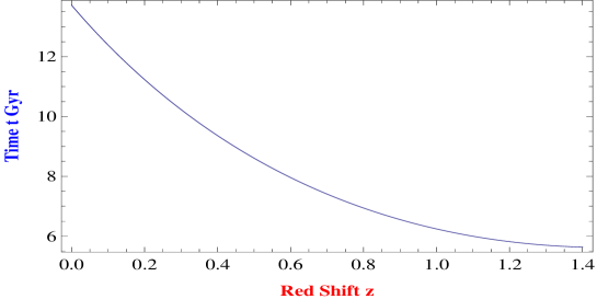
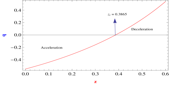
(i) $\chi^{2}$ for Hubble Parameter:

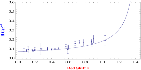
We present following table which describe observed values of Hubble parameter along with error and corresponding theoretical results obtained as per our model in the range ($0\leq z\leq 1$).

Table-1

$\begin{array}[]{|c|c|}\hline\cr{\bf{z}}~{}=~{}0.07,~{}0.1,~{}0.12,~{}0.17,~{}0.179,~{}0.199,~{}0.2,~{}0.27,~{}0.35,~{}0.352,~{}0.4,~{}0.44,~{}0.48,~{}0.57,\\ ~{}0.593,~{}0.6,~{}0.781,~{}0.875,~{}0.88,~{}0.9,~{}1.037\\ \hline\cr{\bf{H_{ob}}}~{}=~{}0.0746,~{}0.0787,~{}0.0908,~{}0.0846,~{}0.0848,~{}0.0971,~{}0.0844,~{}0.0991,~{}0.1064,~{}0.0899,\\ 0.0934,~{}0.0989,~{}0.1073,~{}0.1278,~{}0.092,~{}0.1196,~{}0.1636,~{}0.181,~{}0.1432,~{}0.2066,~{}0.1907\\ \hline\cr{\bf{H_{er}}}~{}=~{}~{}0.0302,~{}0.0143,~{}0.0374,~{}0.0085,~{}0.0143,~{}0.0173,~{}0.0079,~{}0.0634,~{}0.0132,~{}0.0062,\\ ~{}0.0081,~{}0.0071,~{}0.0122,~{}0.0173,~{}0.0409,~{}0.0235,~{}0.0343,~{}0.0184,~{}0.0143,~{}0.0409,~{}0.0515\\ \hline\cr{\bf{H_{th}}}~{}=~{}0.0723,~{}0.0734,~{}0.0741,~{}0.0762,~{}0.0765,~{}0.0774,~{}0.0774,~{}0.0808,~{}0.0851,~{}0.0852,{}\\ 0.0882,~{}0.0909,~{}0.0931,~{}0.1014,~{}0.1036,~{}0.1043,~{}0.1274,~{}0.1452,~{}0.1463,~{}0.1509,~{}0.1942\\ \hline\cr\end{array}$

The observed values and error are taken from a latest paper by Farook at el. [60]. The Hubble data’s are converted into $Gyr^{-1}$ unit. In order to get quantitative closeness of theory and observation, we obtain $\chi^{2}$ from the following formula

$$\chi^{2}=\frac{(H_{ob}-H_{th})^{2}}{H_{er}^{2}}$$

It comes to $19.41469$ which is $92.45\%$ over 21 data’s, which shows best fit in theory and observation. We present following fig. to display this closeness.

Figure 3: Error bar plot of Hubble parameter $H$ showing proximity of theory and observation.

(ii) DE Parameter $\Omega_{de}$ and EoS $\omega_{de}$

Now, from Eqs. (7)-(9), the DE parameter $\Omega_{de}$ and EoS parameter $\omega_{de}$ are given by the following equations and are solved numerically.

$$H^{2}\Omega_{de}=H^{2}-(\Omega_{m})_{0}H^{2}_{0}(1+z)^{3}$$ (14)

$$\omega_{de}=\frac{H^{2}(2\alpha H+2\beta-1)}{3[H^{2}-H_{0}^{2}(\Omega_{m})_{0}(1+z)^{3}]}.$$ (15)

where we have taken $(\Omega_{k})_{0}=0$ for the present spatially flat universe. We solve Eqs. (14) and (15) with the help of Eq. (12) and present the following figures $4$ and $5$ to illustrate the solution.

Figure 4: Plot of $\Omega_{de}$ versus red shift ($z$). This is drawn by solving Eq. (14) and Eq. (12). $H_{0}=0.07Gyr^{-1}$ and $\Omega_{m0}$=0.279 .

Figure 5: Plot of $\omega_{de}$ versus $z$. This is drawn by solving Eq. (15) and Eq. (12). Figure shows that this is a quintessence model.

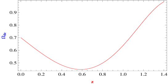
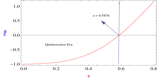
The figures show that this is a quintessence model $\omega_{(de)}\geq-1$ which remains for the period $(0\leq z\leq 0.5806)$. DE favors deceleration at $z\geq 0.5806$ and will help in structure formation at $z\geq 4$. As per our model, the present value of DE parameter is $0.7$. It decreases over the past, attains a minimum value $\Omega_{de}\sim 0.45$ at $z\sim 0.6$, and then it again increases with red shift. It is interesting to note that the growth of EoS parameter for DE $\Omega_{de}$ over red shift during quintessence regime is matching with the pioneering work by Steinhardt et al. [61] and Johri [62]

We look carefully Fig. $4$ in context of Fig. $5$. In fact as per Fig. $5$, the transition red shift is $z_{te}=0.5806$. As we expressed in our explanation, dark energy will begin its roll of opposing deceleration and favoring acceleration during $0\leq z\leq 0.5806$. Before, i.e., $z\geq 0.5806$, $\omega_{de}$ is positive, so dark energy favours deceleration. We may say that the validity of Fig. $4$ is only during the said tenure $0\leq z\leq 0.5806$. During this DE always increases with time. This feature provides a possible way out for the coincidence problem affecting many quintessence models. Unfortunately this the scenario is still affected by the cosmological coincidence problem (CCP) [63].

(iii) Luminosity Distance:

The red shift-luminosity distance relation [64] is an important observational tool to study the evolution of the universe. The expression for the luminosity distance ($D_{L}$) is obtained in term of red shift as the light coming out of a distant luminous body gets red shifted due to the expansion of the universe. We determine the flux of a source with the help of luminosity distance. It is given as $D_{L}=a_{0}r(1+z).$ where r is the radial coordinate of the source. For the FLRW metric Eq. (2), the radial co-ordinate $r$ is obtained as $r=\int^{r}_{0}dr=\int^{t}_{0}\frac{cdt}{a(t)}=\frac{1}{a_{0}H_{0}}\int^{z}_{0}\frac{cdz}{h(z)},$ where we have taken $k=0$ and have used $dt=dz/\dot{z},\dot{z}=-H(1+z)~{}\&~{}h(z)=\frac{H}{H_{0}}.$ Therefore, we get the luminosity distance as:

$$\frac{H_{0}D_{L}}{c}=(1+z)\int^{z}_{0}\frac{dz}{h(z)}.$$ (16)

(iv) Distance modulus $\mu$ and Apparent Magnitude $m_{b}$:

The distance modulus $\mu$ [12] is derived as

$$\mu=m_{b}-M=5log_{10}\left(\frac{D_{L}}{Mpc}\right)+25=25+5log_{10}\left[\frac{c(1+z)}{H_{0}}\int^{z}_{0}\frac{dz}{h(z)}\right]$$ (17)

The absolute magnitude $M$ of a supernova [12] is $M=16.08-25+5log_{10}(H_{0}/.026c)$. Using this, the apparent magnitude $m_{b}$ is obtained as

$$m_{b}=16.08+5log_{10}\left[\frac{1+z}{.026}\int^{z}_{0}\frac{dz}{h(z)}\right].$$ (18)

We solve Eqs. (16)$-$ (18) with the help of Eq. (12). Following is the value of the integral

$$\int^{z}_{0}\frac{dz}{h(z)}\simeq(1.25z+0.09(1-(1.+z)^{2.76})$$

(v) $\chi^{2}$ for Distance Modulus ‘$\mu$’:

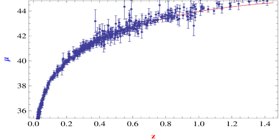
Our theoretical results have been compared with SNe Ia related $581$ data’s from Pantheon compilation [58] with possible error in the range ($0\leq z\leq 1.3$.) and the derived model was found to be in good agreement with current observational constraints. In order to get quantitative closeness of theory and observation, we obtain $\chi^{2}$ from the following formula

$$\chi^{2}=\frac{(\mu_{ob}-\mu_{th})^{2}}{\mu_{err}^{2}}$$

It comes to $562$ which is $96.73\%$ over $581$ data’s, which shows best fit in theory and observation. The following figures $8$ depict the closeness of observational and theoretical results, thereby justifying our model.

Figure 6: Plot of distance modulus ($\mu=M-m_{b}$) versus red shift ($z$). Crosses are SNe Ia related Pantheon compilation $581$ data’s with possible corrections, $H_{0}$ = 0.07 $Gyr^{-1}$, $\Omega_{m0}$ = 0.279 and $\Omega_{\Lambda 0}$ = 0.721.

4 Conclusion:

In the present paper, we have presented an FLRW universe filled with two fluids (barotropic and dark energy), by assuming DP as a linear function of the Hubble constant. This results in a time-dependent DP having a transition from past decelerating to the present accelerating universe. The main findings of our model are itemized point-wise as follows.

• The expansion of the universe is governed by a expansion law $q=\alpha H+\beta,~{}H=-\frac{A(\beta+1)(z+1)^{\beta+1}}{0.07\left(A\alpha(z+1)^{\beta+1}-1\right)}$, where $\alpha=31.619,\beta=-2.76333$ and A = 0.15. This describes the transition from deceleration to acceleration.

• The transition red shift is $z_{t}=0.386$ and corresponding time is $T_{t}=1.034$ Gigayear. The universe is now accelerating and it was decelerating before time $T_{t}$

• This is a quintessence model $\omega_{(de)}\geq-1$ which remains for the period $(0\leq z\leq 0.5806)$. DE favors deceleration at $z\geq 0.5806$.

• the present value of DE parameter is $0.7$. It decreases over the past, attains a minimum value $\Omega_{de}\sim 0.45$ at $z\sim 0.6$, and then it again increases with red shift.

• The growth of EoS parameter for DE $\Omega_{de}$ over red shift during quintessence regime is matching with the pioneer work by Steinhardt et al. [61] and Johri [62].

• In the present model dark energy doe not interact with a barotropic fluid. We have observed that for both cases, interacting and non-interactiong, the graphs come to be the same. It indicates that the dark energy component is so dominated that, its interaction with barotropic fluid does not affect the non-interacting scenario. So, we have only discussed the non-interacting model.

• It is to mention here that that the assumption of deceleration parameter $q$ as a function of $H$ is adhoc in the sense that it does not result from known field theory. However, it does produce a solution that presents an appropriate description of the universe consistent with observations. The agreement with the observed universe is just qualitative.

• Our model is compatible with current observations. We have discussed it in different places with appropriate motivations and their references.

• In Fig. $4$, we observe that $\Omega_{de}$ does not always increase. It is minimum at red shift $\approx 0.6$. If we parametrize the expansion of the Universe in terms of red shift $z$, it appears a particular period of cosmic history as density ration of DM and DE of order of one. This scenario at low value of $z$ suggests that the dominance of DE started “recently” or even “now” on cosmological scale, giving rise to the CCP “why now?” [63].

In a nutshell, we believe that proposed linear law may help in investigations of hidden matter like dark matter, dark energy and black holes.

References

- [1] A. Sandage, Physics Today 34, (1970).
- [2] S. Perlmutter et al., Astrophys. J. 517, 5 (1999).
- [3] A. G. Riess et al., Astron. J. 116, 1009 (1998).
- [4] A. Clocchiatti et al., Astrophys. J. 642, 1 (2006).
- [5] P. de Bernardis et al., Nature 404, 955 (2000).
- [6] S. Hanany et al., Astrophys. J. 493, L53 (2000).
- [7] D. N. Spergel et al., Astrophys. J. Suppl. 148, 175 (2003).
- [8] N. Suzuki et al., Astrophys. J. 746, 85 (2011).
- [9] T. Delubac et al., Astron. Astrophys. 574, A59 (2015).
- [10] C. Blake et al., Mon. Not. R. Astron. Soc. 425, 405 (2012).
- [11] P. A. R. Ade et al., Astron. Astrophys. 594, A14 (2016).
- [12] E. J. Copeland et al., Int. J. Mod. Phys. D 15, 1753 (2006).
- [13] D. Huterer and M. S. Turner, Phys. Rev. D 64, 123527 (2001).
- [14] J. Weller and A. Albrecht, Phys. Rev. D 65 , 103512 (2002).
- [15] D. Polarski and M. Chevallier, Int. J. Mod. Phys. D 10, 213 (2001).
- [16] E. V. Linder, Phys. Rev. Lett. 90, 91301 (2003).
- [17] T. Padmanabhan and T.P. Roy Choudhury, Mon. Not. R. Astron. Soc. 344, 823 (2003).
- [18] P.S. Corasaniti et al., Phys. Rev. D 70, 083006 (2004).
- [19] U. Alam, JCAP 0406, 008 (2004)
- [20] U. Alam et al., Mon. Not. Roy. Astron. Soc. 344, 1057 (2003).
- [21] H. Amirhashchi, A. Pradhan and B. Saha, Chin. Phys. Lett. 28, 039801 (2011).
- [22] H. Amirhashchi, A. Pradhan and H. Zainuddin, Int. J. Theor. Phys. 50, 3529 (2011).
- [23] A. Pradhan, H. Amirhashchi and B. Saha, Astrophys. Space Sci. 333, 343 (2011).
- [24] B. Saha, H. Amirhashch and A. Pradhan, Astrophys. Space Sci. 342, 257 (2012).
- [25] A .Pradhan, Indian J. Phys. 88, 215 (2014).
- [26] S. Kumar, Astrophys. Space Sci. 332, 449 (2011).
- [27] A. A. Coley and B. O. J. Tupper, Jour. Math. Phys. 27, 406 (1986).
- [28] A. A. Coley, Astrophys. Space Sci. 140, 175 (1988).
- [29] A. Gromov, Yu. Baryshev and P. Teerikorpi, Astron & Astrophys. 415 813 (2004).
- [30] M. R. Setare, J. Sadeghi and A. R. Amani, Phys. Lett. B 673, 241 (2009).
- [31] M. Jamil, E. N. Saridakis and M. R. Setare, Phys. Rev. D 81, 023007 (2010).
- [32] T. Singh and R. Chaubey, Res. Astron. Astrophys. 12, 473 (2012).
- [33] T. Singh and R. Chaubey, Canad. J. Phys. 91, 180 (2013).
- [34] D. R. K. Reddy and R. S. Kumar, Int. J. Theor. Phys. 52, 1362 (2013).
- [35] P. Garg, R. Zia and A. Pradhan, Int. J. Geom. Methods Mod. Phys. 16, 1950007 (2019).
- [36] G. K. Goswami, A. Pradhan and A. Beesham, arXiv:1906.00450[gr-qc], Accepted in Pramana-J. Phys. (2019).
- [37] V. J. Dagwal and D. D. Pawar, Int. J. Math. Archive 9(2), 120 (2018), arXiv:1704.07107[gr-qc].
- [38] O. Akarsu et al., Jour. Cosm. Astrophys. 01, 022 (2014).
- [39] D. Huterer and M. S. Turner, Phys. Rev. D 64, (2001); astro-ph/0012510.
- [40] J. Weller and A. Albrecht, Phys. Rev. D 65, 103512 (2002) ; astro-ph/0106079.
- [41] M. Chevallier and D. Polarski, Int. J. Mod. Phys. D 10, 213 (2001), gr-qc/0009008.
- [42] E.V. Linder, Phys. Rev. Lett. 90, 91301 (2003), astro-ph/0402503.
- [43] H. K. Jassal, J. S. Bagla and T. Padmanabhan, MNRAS 356, 611(2005); astro-ph/0404378;
- [44] T. Padmanabhan and T. Roy Choudhury, MNRAS 344, 823 (2003); astro-ph/0212573
- [45] A. Upadhye, M. Ishak and P. Steinhardt, Phys. Rev. D. 72, 063501 (2005) ; astro-ph/0411803.
- [46] S. Hannestad and E. M ortsell, JCAP 0409, 001 (2004); astro-ph/0407259.
- [47] S. Lee, Phys. Rev. D 71, 123528 (2005); astro-ph/0504650.
- [48] F. F. R. Ellis and M. Madsen, Class. Quantum Grav. 8, 667 (1991).
- [49] N. Banerjee and S. Das, Gen. Relativ. Gravit. 37, 1695 (2005).
- [50] J. P. Singh, Astrophys. Space Sci. 318, 103 (2008).
- [51] J. P. Singh, Int. J. Theor. Phys. 48, 2041 (2009).
- [52] R. Zia, D. C. Maurya and A. Pradhan, Int. J. Geom. Methods Mod. Phys. 15, 1850168 (2018).
- [53] P. Garg, R. Zia and A. Pradhan, Int. J. Innov. Techn. Explor. Engin. (IJITEE) 8, 1758 (2019).
- [54] U. K. Sharma, R. Zia and A. Pradhan, Res. Astron. Astrophys. 19, 55 (2019).
- [55] R. K. Tiwari, R. Singh and B. K. Shukla, African Rev. Phys. 10, 0048 (2015).
- [56] R. K. Tiwari, A. Beesham and B. K. Shukla, Int. J. Geom. Methods Mod. Phys. 15, 1850189 (2018).
- [57] H. Amirhashchi and S. Amirhashchi arXiv:1811.05400v4 (2019).
- [58] D. M. Scolnic, Astrophys. J. 859, 101 (2018).
- [59] M. Betouleet al., Astron, Astrophys. 568, A22(2014).
- [60] O. Farooq et al., Astrophys. J. 835, 26 (2017).
- [61] P. Steinhardt, L. Wang and I. Zlatev, Phys. Rev. D 59, 123504 (1999).
- [62] V. B. Johri, Phys. Rev. D 63, 103504 (2001).
- [63] H. E. S. Velten, R. F. vom Marttens and W. Zimdahl, Eur. Phys. J. C 74, 11 (2014), 3160 arXiv:1401.2509[astro-ph.CO].
- [64] A. R. Liddle and D. H. Lyth, Cosmological Inflation and Large-Scale Structure (Cambridge University Press, 2000).