Outliers of random perturbations of Toeplitz matrices with finite symbols
Anirban Basak∗∗International Centre for Theoretical Sciences
Tata Institute of Fundamental Research
Bangalore 560089, India
and Ofer Zeitouni§§Department of Mathematics, Weizmann Institute of Science
POB 26, Rehovot 76100, Israel
and
Courant Institute, New York University
251 Mercer St, New York, NY 10012, USA
Abstract.
Consider an Toeplitz matrix with symbol , perturbed by
an additive noise matrix ,
where the entries of are centered
i.i.d. random variables of unit variance and .
It is known that the empirical measure of eigenvalues
of the perturbed matrix converges weakly, as , to the law of , where is distributed uniformly on .
In this paper, we consider the outliers, i.e. eigenvalues that are at a positive (-independent) distance from . We prove that there are no outliers outside , the spectrum of the limiting Toeplitz operator, with probability approaching one, as . In contrast, in the process of outliers converges to the point process described by the zero set of certain random analytic functions. The limiting random analytic functions can be expressed as linear combinations of the determinants of finite sub-matrices of an infinite dimensional matrix, whose entries are i.i.d. having the same law as that of . The coefficients in the linear combination depend on the roots of the polynomial and semi-standard Young Tableaux with shapes determined by the number of roots of that are greater than one in moduli.
1. Introduction
Let be a Laurent polynomial. That is,
(1.1)
for some and some sequence of
complex numbers , so that 111We remark that if one is interested in the case where but ,
one may simply consider, when computing spectra, the transpose of or of . For this reason, the restriction to does not reduce
generality..
Define
to be the Toeplitz operator with symbol , that is the operator given by
and we set for non-positive integer values of .
For , we denote by the natural -dimensional truncation of the infinite dimensional Toeplitz operator . As a matrix of dimension , we have
(for ) that
In general, is not a normal matrix, and thus its spectrum can be sensitive
to small perturbations. In this paper, we will be interested in the spectrum of
, where is a “vanishing” random perturbation, and especially in
outliers, i.e. eigenvalues that are at positive distance from the limiting spectrum.
Let denote the empirical measure of eigenvalues of , i.e.
, where is the Dirac measure at .
It has been shown in [3] that under a fairly general condition on the (polynomially vanishing)
noise matrix , converges (weakly, in probability) to
,
where denotes the Haar measure on .
That is, the limit is the law of
where (see also [20] for the case of Gaussian noise).
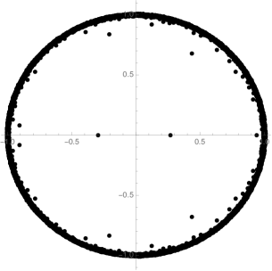
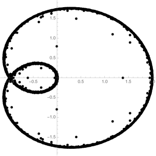
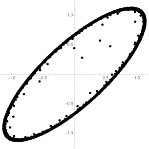
However, simulations (see Figure 1) suggest
that although the bulk of the eigenvalues approach , as , there are a few eigenvalues of
that wander around outside a small neighborhood of
. Following standard terminology, we call them outliers. The goal of this paper is to characterize these outliers.
Figure 1.
The eigenvalues of , with , , a real Ginibre matrix, and various symbols . On the top
left,
. On the top right, . On the
bottom, .
In simulations depicted in
Figure 1, all eigenvalues of
, where and is a standard real Ginibre matrix, are inside the unit disk, the limaçon, and the ellipse when the symbol is , and , respectively. It follows from standard results on the spectrum of Toeplitz operators, e.g. [7, Corollary 1.12] that these regions are precisely , the spectrum of the Toeplitz operator
acting on .
Thus, Figure 1 suggests that there are no outliers outside . In our first result, Theorem 1.1 below, we confirm this and prove the universality of this phenomenon for any finitely banded Toeplitz matrix, , and under a minimal assumption on the entries of the noise matrix.
We introduce the following standard notation: for and , let be the -fattening of . That is, , where . Further denote .
Theorem 1.1.
Let be a Laurent polynomial. Let
denote
the Toeplitz operator on with symbol ,
and let be its natural -dimensional projection.
Assume for some , where the entries of are independent (real or complex-valued) with zero mean and unit variance.
Further, let
denote the empirical measure of eigenvalues of . Fix . Then,
(1.2)
In the terminology of [20],
is a
zone of spectral stability for .
The following remarks discuss some generalizations and extensions of Theorem 1.1.
Remark 1.2.
For clarity of presentation, in Theorem 1.1 we assume the entries of to have a unit variance. The
proof shows that the same conclusion continues to hold under the assumption that the entries of are jointly independent (possibly having -dependent distributions), and have zero mean and uniformly bounded second moment, i.e.
(1.3)
where denotes the -th entry of .
We emphasize that under the general assumption (1.3) on the entries of ,
one may not have the convergence of the empirical measure of the eigenvalues of to . Theorem 1.1 shows that even under such perturbations there are no eigenvalues in the complement of .
Remark 1.3.
The proof of Theorem 1.1 shows that its conclusion
continues to hold if , with
any sequence such that (the standard notation means that ). For conciseness, we only consider .
Remark 1.4.
Theorem 1.1 shows that, with probability approaching one, all eigenvalues of the random perturbation of are contained in an -fattening of the spectrum of
the infinite dimensional Toeplitz operator . Here we have chosen to work with a fixed parameter . With some additional efforts it can be shown that in (1.2) one can allow to decay to zero slowly with . We do not pursue this direction.
Remark 1.5.
The ideas used to prove Theorem 1.1 also show that
the sequence is tight, where is the spectral radius (maximum modulus eigenvalue) of , with as in Theorem 1.1. See Proposition A.1. It has been conjectured in [6] that the spectral radius of a matrix with i.i.d. entries of zero mean and variance converges to one, in probability. Thus Proposition A.1 proves a weaker form of this conjecture.
Remark 1.6.
In [20, Proposition 3.13], the authors show that the resolvent of remains bounded in compact subsets of .
As noted in [20],
this implies Theorem 1.1 in the Gaussian case because
in that case, the operator norm of is bounded with high probability. For more general perturbations possessing only four or less moments, the operator norm of is in general not bounded, for some , and a similar argument fails.
We turn to the identification of
the limiting law of the random point process consisting
of the outliers of ,
which by
Theorem 1.1 are contained in . Before stating the
results, we review
standard
definitions of random point processes and their notion of convergence, taken from
[10].
For we let denote the Borel -algebra on it. Recall that a Radon measure on is a measure that is finite for all Borel compact subsets of .
Definition 1.1.
A random point process on an open set is a probability measure on the space of all non-negative integer valued Radon measures on . Given a sequence of random point processes on , we say that converges weakly to a (possibly random) point process on the same space, and write , if for all compactly supported bounded real-valued continuous functions ,
when viewed as real-valued Borel measurable random variables.
Next we proceed to describe the limit. We will see below that the limit is given by the zero set a random analytic function, where the description of the limiting random analytic function differs across various regions in the complex plane. This necessitates the following definition.
Definition 1.2(Description of regions).
For any
Laurent polynomial as in (1.1), set . Writing , let be the roots of the equation arranged in an non-increasing order of their moduli.
For an integer such that , set
where for convenience we set and for all .
Note that for all roots of the polynomial have moduli different from one. Therefore for such values of , is well defined, and hence so is .
By construction, .
Since, by [3], the bulk of the eigenvalues of
approaches in the large limit, to study the outliers we only need to analyze the roots of that are in .
Before describing the limiting random field let us mention some relevant properties of the regions . As is a Laurent polynomial satisfying (1.1) it is straightforward to check that for we have , where denotes the winding number about of the closed curve induced by the map for . Thus splits the complement of according to the winding number. Moreover, as will be seen later, the description of the law of the limiting random point process differs across the regions .
Furthermore, from [7, Corollary 1.12] we have that
It was noted above that for . So
(1.4)
Hence in light of Theorem 1.1 we conclude that
to find the limiting law of the outliers it suffices to analyze the
eigenvalues of that are in .
Finally, we note that from the continuity of the roots of in in the symmetric product topology (see [27, Appendix 5, Theorem 4A]) it follows that the regions are open, and hence by Definition 1.1 the random point processes on those regions are well defined.
Remark 1.7.
We highlight that one or more of the regions may be empty. For example, when the product of the moduli of the roots of is . So both roots of cannot be less than one in moduli. Therefore in this case. It can be checked that under this same set-up and are the outside and the inside of the ellipse, respectively, in the bottom panel of Figure 1.
Furthermore, if with then both and are empty.
Fix an integer such that . As mentioned above, the limiting random point process in will given by the zero set of a
random analytic function to be defined on . The function can be written as a linear combination of determinants of sub-matrices of the noise matrix, where the coefficients depend on the roots of the polynomial and semistandard Young Tableaux of some given shapes with certain restrictions on its entries. We recall
the definition of semistandard Young Tableaux [22, Section 7.10].
Definition 1.3(Semistandard Young Tableaux).
Fix . A partition with parts is a collection of non-increasing non-negative integers
. Given a partition , a semistandard Young Tableaux of shape is an array of positive integers of shape (i.e. and ) that is weakly increasing (i.e. non-decreasing) in every row and strictly increasing in
every column.
The limiting random field depends on the following subset of the set of all semistandard Young Tableaux, for which we have not found a standard terminology in the literature.
Definition 1.4(Field Tableaux).
Let be a partition with and . For an integer such that , let
denote the collection of all semistandard Young Tableaux of shape
that are strictly increasing along the southwest diagonals and satisfies the assumption for all . See Figure 2 for a pictorial illustration.
Equipped with the relevant notion of semistandard Young Tableaux we now turn to define the coefficients that appear when the limiting random analytic function is expressed as a linear sum of determinants of sub-matrices of the noise matrix.
Definition 1.5(Field notation).
Fix an integer such that . Set . For any finite set ,
we define to be the sign of the permutation which places all elements of before those
in but preserves the order of the elements within the two sets.
Figure 2. Examples of (left column) and (right column) with , where , , and for are as in Definition 1.5. , . Top and bottom rows are and , respectively.
For the top row
and for the bottom row
Having defined all necessary ingredients we now introduce the limiting random analytic function .
Definition 1.6(Description of the random fields).
Let denote a semi-infinite array of i.i.d. random variables with zero mean and unit variance. For , let denote the sub-matrix of induced by the rows and the columns indexed by
and , respectively. With notation for ,, and as in Definition 1.5,
we set, for and ,
(1.6)
It may not be apriori obvious from Definition 1.6 that is well defined,
as (1.6) is an infinite sum.
Lemma 1.9 below will establish that it can be expressed as the local uniform limit of the random analytic functions and thus it is indeed a well defined random analytic function. In addition, under an
appropriate anti-concentration property of the entries of
and , the random analytic function is not identically zero on a set of probability one, and thus
the random point process induced by the zero set of it
is a valid random Radon measure.
To describe the required anti-concentration property, we recall
Lévy’s concentration function, defined for any
(possibly complex-valued) random variable by
Equipped with the above definition we now state the additional
assumption on the entries of and .
Assumption 1.8(Assumption on the entries of the noise matrix).
Assume that the entries of and are either real-valued or complex-valued i.i.d. random variables with zero mean and unit variance, so that, for some absolute constants and ,
(1.7)
for all sufficiently small , where is the first diagonal entry of .
Note that any random variable having a bounded density with respect to the Lebesgue measure on the real line, and the complex plane satisfies the bound (1.7) with and , respectively. This in particular includes the standard real and complex Gaussian random variable.
Recall that a sequence of complex-valued functions , defined on some open set , is said to converge locally uniformly to a function , if given any there exists some open ball containing such that converges to uniformly on , as .
We now have the following.
Lemma 1.9(Description of the limit).
Let , , and be as in Definition 1.6. We let be the random point process induced by the zero set of the random field . That is,
(1.8)
Then we have the following:
(i)
The functions are random analytic functions.
(ii)
The random function is well defined
on a set of probability one. Furthermore, converges locally uniformly to , almost surely, as , and hence is a random analytic function.
(iii)
Under the additional
Assumption 1.8, the random function is almost surely non constant.
Recalling Definition 1.1 we note that the notion of convergence of random point processes defined on is tested against continuous functions supported on compact subsets of . Therefore when discussing convergence it is enough to consider continuous functions on sets for arbitrary .
Remark 1.10.
We emphasize that the random point process , although free of the parameter , is not universal. That is, in general its law depends on the law of the entries of the matrix .
The main result of this paper shows that given an integer such that and ,
the random point process induced by the eigenvalues of that are in converges weakly to the random point process induced by the zero set of the random analytic function .
Theorem 1.11.
Let be a Laurent polynomial as in (1.1).
Let denote
the Toeplitz operator on with symbol ,
and let be its natural -dimensional projection.
Assume for some , where the entries of are
i.i.d. satisfying Assumption 1.8. Furthermore assume that the
entries of in Definition 1.6
are i.i.d. of the same law
as that of the entries of
.
For any
integer such that ,
let denote
the random point process induced by the eigenvalues of that are in . That is,
Then, for such ,
converges weakly, as , to
the random point process from Lemma 1.9.
Explicit expressions for the fields in the
statement of Theorem 1.11 for two of the
symbols depicted in Figure 1 appear in Section 1.1 below,
see (1.9) and Remark 1.13.
At a first glance, it may seem counter intuitive for the limit to be expressed as the zero set of certain random analytic function of the form (1.6). To see that it is in fact natural, we note that the determinant of can be expressed as
a linear combination of products of determinants of
sub-matrices of and of , and further
that the determinants of (some) sub-matrices of a finitely
banded Toeplitz matrix can be expressed as certain
skew-Schur polynomials in (see [1, 9]),
where these polynomials are defined as a sum of monomials with the sum taken over (skew) semistandard Young Tableaux of some given shapes. This leads to
(1.6).
Remark 1.12.
As before, when discussing convergence it is enough to consider functions supported on the sets
for arbitrary . Similar to Remark 1.4, one can allow in Theorem 1.11 to go to zero, as , sufficiently slowly, and consider functions supported on as test functions. We do not work out the details
here.
1.1. Background, related results, and extensions
The fact that the spectrum of non-normal matrices and operators
is not stable with respect
to perturbations is well known, see e.g. [23] for a
comprehensive account and [11]
for a recent study. Extensive work has been done concerning worst case perturbations, which are captured through the notion of pseudospectrum. However, beyond some specific examples the pseudospectrum of non-normal operators are not well characterized. Hence, in recent times there have been growing interests in studying the spectrum of non-normal operators and matrices under small typical perturbations. See the references in [17, Section 1]. We also refer to [2, Section 1.3] for a discussion about the relation between the pseudospectrum and the spectrum under typical perturbation, and an extensive reference list. We add that early examples of the spectrum obtained by noisily perturbing Toeplitz matrices with finite symbols appeared in [24].
As mentioned above, the convergence of the empirical measure of eigenvalues for randomly perturbed finite-symbol Toeplitz matrices has now been established in
great generality, see the recent articles [3, 20] and references therein. Our focus in this paper concerns the study of outliers. In Theorem 1.1 we identify the region where no outliers are present (in the terminology of Sjöstrand and Vogel [20], this
is the
zone of spectral stability).
Then, in Theorem 1.11 we find the limit of the random processes induced by the outliers in the interior of the complement of the region identified in Theorem 1.1.
For the Jordan matrix, i.e. the Toeplitz matrix with symbol , [11, Theorem 2] shows that there are no outliers outside the unit disc (centered at zero) in the complex plane, with high probability. In the general Toeplitz case, Theorem 1.1 follows
(for Gaussian perturbations)
from the resolvent estimates in [20, Proposition 3.13], see Remark 1.6.
Some bounds on the number of outliers inside
are available in the literature. In the notation of the current
paper, for the Jordan matrix perturbed by additive complex Gaussian noise, with
, a logarithmic in bound
for the number of outliers appears in
[11]. Similar results (with worse error bounds) are given in [17] for non-triangular tridiagonal Toeplitz matrices (i.e. the symbol is ), and in [20] for general Toeplitz matrices with finite symbol.
Sharper results concerning
outliers for the Jordan matrix and the non-triangular tridiagonal Toeplitz matrix (under complex Gaussian perturbation),
are presented in [18, 19]. In both these cases, a sharp control on the number of outliers in the regions with is
provided. In the language of the current paper, the authors compute the first intensity measure of the limiting field
, that is, they compute the function for subsets .
For
the Jordan matrix, it has been shown in [19, Theorem 1.1] that has a density with respect to the two dimensional Lebesgue measure,
given by
Due to the
Edelman-Kostlan formula (see [12, Theorem 3.1]),
is the first intensity measure of the random point process induced by the zero set of the hyperbolic Gaussian analytic function (see [13, Chapter 2.3] for a definition), given by
(1.9)
where are i.i.d. standard complex Gaussian random variables.
We now explain how to recover this result from Theorem
1.11: in the case of the Jordan matrix, and then , and .
Substituting in Definition 1.5, one finds that
where are arbitrary positive integers. In particular, there are
precisely choices of such integers that give .
Since the entries of are i.i.d. Gaussian, it follows from
(1.6) that coincides with
(1.9). Together with the Edelman-Kostlan formula, this
recovers [19, Theorem 1.1]. Note that the same expression (1.9)
also holds
for real Gaussian noise, with the limiting field having now real Gaussian coefficients.
Remark 1.13.
Theorem 1.11 allows one to describe
all limiting outlier processes for the other cases depicted in
Figure 1. We give one more example, for the symbol
(the “limaçon”),
with Gaussian noise matrix consisting of i.i.d. centered entries.
There, we have that ,
arranged so that .
In the region , which corresponds to the region
enscribed by the limaçon curve with winding number ,
the limiting field is
(1.10)
where are i.i.d. centered Gaussian,
compare with (1.9). On the other hand, in the regions
(which corresponds to the region of winding number 2, i.e. the smaller
region in Figure 1), the limiting field admits a more complicated
description, as follows. Let be i.i.d.
Gaussians, and for integers satisfying and ,
introduce
the random variables
and the
functions
Then,
(1.11)
In particular, the random coefficients in (1.11)
are in general not Gaussian, and
there are terms in the sum in (1.11) with non-trivial
correlations.
Sjöstrand and Vogel in [18] compute
for the non-triangular tridiagonal Toeplitz matrix.
Again by the Edelman-Kostlan formula, they identify
with the first intensity measure of the random point
process induced by the zero set of some Gaussian analytic
function with some covariance kernel .
Our Theorem 1.11,
when applied to non-triangular tridiagonal Toeplitz matrix, again
shows that under complex Gaussian perturbation the
limiting random fields are the zero sets of Gaussian analytic functions,
and a computation (which we omit) shows that its covariance
kernel is given by .
Thus, Theorem 1.11 again recovers the results
of [18].
We also mention the relevant work [14], where local statistics
for the
eigenvalues of
random perturbations of certain pseudo-differential operators are computed
and related to local statistics of the zeros of random Gaussian analytic
functions.
Based on [18, 19, 14] one may be tempted to predict that for general finitely banded Toeplitz matrices the limiting random field is the zero set of some Gaussian analytic function. Theorem 1.11 shows that, even under complex Gaussian perturbations, the limit may not be the zero set of Gaussian analytic functions, e.g. consider and the limit of the random point process induced by the outlier eigenvalues in . Furthermore, even in the framework of [18, 19], under general perturbation, as already mentioned in Remark 1.10, the limit turns out to be non-universal.
The work of Śniady [21] considers situations where the
additive noise is Gaussian of standard deviation , and deals
with the limit where first and then .
Some of the subsequent work, reviewed e.g. [2, Section 1.4],
can
be seen as an attempt to modify the order of limits. In this direction and
concerning outliers,
Bordenave and Capitaine [5] study outliers of
deformed i.i.d. random matrices. Namely, for a sequence of deterministic matrices they study the outlier eigenvalues of , where the entries of are i.i.d. complex-valued random variables satisfying some assumptions on its moments, and is a parameter. When is the Jordan matrix, in [5, Corollary 1.10] it is shown that for any the random point process induced by the outlier eigenvalues of converges to the zero set of a Gaussian analytic function with some covariance kernel . They also noted that, as , the kernel admits a non-trivial limit and the limiting kernel turns out to be the covariance kernel of the hyperbolic Gaussian analytic function given by (1.9).
It is striking to see that for the complex Gaussian perturbation of the Jordan matrix the same limit appears in these two rather different frameworks: in [5] is followed by , whereas in this paper and are sent to infinity together with for some . However, it should also be noted that, unlike [5], here the limit is non-universal. Based on this observation, we predict that the same phenomenon should continue to hold for general finitely banded Toeplitz matrices.
Next, we discuss possible
extensions of our results.
A first obvious direction is to consider
in Theorem 1.11 the case of without the density assumption. Many steps of the proof go through, except for anti-concentration results of the type discussed
in Section 4. As will be explained in Section 1.2 below, in Section 4 we derive anti-concentration bounds for linear combinations of determinants of sub-matrices of . To obtain such a bound we use that there is at least one term in the linear sum with a large coefficient.
We conjecture that it should be possible to dispense of any density assumption on the entries of the noise matrix and the conclusion of Theorem
1.11 should continue to hold under minimal assumptions on the entries , e.g. i.i.d. with zero mean and unit variance. At the level of convergence of empirical measures,
this has been verified, first in [26] and then in [3]. The non-universality of the limit process for outliers, see Remark 1.10,
complicates however the task of proving this.
The next section outlines the proofs of Theorems 1.1 and 1.11.
1.2. Outline of the proof
We remind the reader that the bulk of the eigenvalues of approach the curve , as . Thus, to study the outlier eigenvalues we need to analyze the set , where for brevity, hereafter we denote and recall the definition of from Definition 1.2.
To this end, a key observation is that for the dominant term in the expansion of is , where for , is the homogeneous polynomial of degree in the entries of the noise matrix in the expansion of the determinant (see (2.1) for a precise formulation, and (2.2) for
a decomposition of the determinant in terms of these polynomials). It suggests that, the roots of that are in should be close to those of . This, in turn, indicates that the limit of the random point process induced by the roots of that are in should be the same for the equation . The proof then boils down to identifying the limit induced by the roots of that are in . The goal of this paper is to make these heuristics precise, leading to
the conclusions of Theorems 1.1 and 1.11.
The heuristics described above can be mathematically formulated as below. We fix , and consider the region .
From [3, Lemma A.1] it follows that the determinant of can be written as a sum of , where runs from zero to .
From [3, Lemma A.3], after some preprocessing, it follows that is a polynomial in such that it is of degree in each variable (see (2.17) below), where we remind the reader that are the roots of the polynomial , see Definition 1.2. Since for we have , it is natural to believe that for large the roots of and of should be close to each other, where is obtained from by removing terms having exponents of and that are less than , and greater than , respectively.
Indeed, we show in Section
2 that the errors made by replacing
the determinant of (which is an analytic function)
by are small (in the sense that the supremum
of the modulus of the difference over , properly
normalized, has small second moment when followed by
). We also prove that are analytic
functions in , see
Lemma 5.1.
The advantage of working with (the normalized form of)
is that, for fixed , it has a law independent of . This fact is a
consequence of a combinatorial analysis, presented in Section
3. The upshot is that , properly
normalized,
can be replaced by the -independent analytic
fields , and these fields
in turn possess a well defined analytic
limit as .
In order to pass from convergence of the fields to convergence of the process of
zeros, we employ a general criteria formulated in
[16]. Namely, we
need to check that the limit field is non degenerate,
i.e. does not vanish identically. Since was obtained
as a limit, it suffices to check that the pre-limit possesses good
enough anti-concentration properties at a fixed
point . The pre-limit for which we
prove anti-concentration is , see Corollary
4.2; the latter builds on an anti-concentration
result for polynomials in independent variables with maximal degree one in each variable, see Proposition 4.1.
The proof of Theorem 1.1 follows a simpler
line of argument. Indeed, we show that now the the term with
is dominant, now for all ,
on a set of probability . Thus the task reduces
to
showing that does not have any root in . Turning to do the same, using an operator norm bound on the noise matrix an -dependent region can be identified to not have any eigenvalue of , with high probability. Hence, one only needs to find a uniform lower bound on the modulus of
for .
Evaluating the determinant of a finitely banded Toeplitz matrix has a long and impressive history. If the roots of are distinct then the determinant of is given by Widom’s formula (see [7, Theorem 2.8] and [4]), whereas in the case of double roots there is an analogous result, known as Trench’s
formula, see [7, Theorem 2.10] and [25] for
a proof. Recently, Bump and Diaconis [9] noted that, irrespective of whether has double roots or not, the determinant of a finitely banded Toeplitz matrix can be expressed as a ratio of certain Schur polynomials in the roots of . Since we are interested in finding a uniform lower bound on the modulus of the determinant we work with the formulation of Bump and Diaconis, from which the desired uniform lower bound follows. This finishes the outline of the proof of Theorem 1.1.
Outline of the rest of the paper
In Section 2, using the second moment method, we find upper bounds on the non-dominant terms. Section
3 presents the combinatorial
analysis leading
to controls of the fields and .
Section 4 is devoted to
deriving the
general anti-concentration bounds alluded to
above, which is then applied to yield the same for the dominant term.
Section 5 is devoted to the proof of
Theorem 1.11, while
Section 6 is devoted to the proof of
Theorem 1.1.
Finally, as mentioned in Remark 1.5,
extending the ideas of proof of Theorem 1.1, in Appendix A we prove that the spectral radii of are tight.
Acknowledgements
Research of AB is partially supported by a grant from Infosys Foundation, an Infosys–ICTS Excellence grant, and a Start-up Research Grant (SRG/2019/001376) and MATRICS grant (MTR/2019/001105) from Science and Engineering Research Board of Govt. of India. OZ is partially supported by Israel Science Foundation grant 147/15 and funding from the European Research Council (ERC) under the European Unions Horizon 2020 research and innovation program (grant agreement number 692452). We thank Mireille Capitaine for her interest and for discussing [5] with us, and thank Martin Vogel for Remark 1.6 and other useful comments. We are grateful to the
anonymous referee for her/his suggestions that led to a
shortening of our original proof of Theorem 1.11,
and
also to a weakening of its hypotheses. We also thank the referee for
several other useful comments.
2. Identification of
dominant term and tightness of the scaled determinants
In this section we show that the determinant of , when scaled appropriately, is uniformly tight, where we remind the reader that and . This will be shown by deriving uniform upper bounds on the non-dominant terms of the scaled determinant, as well as the same for the dominant term. For later use, we will also derive bounds on the second moment of the tail of the dominant term.
Before proceeding further we
introduce relevant definitions. For set
(2.1)
where we recall that
denotes the sub-matrix of induced by the rows in and columns in , , , and for , is the permutation on which places all the elements of before all the elements of , but preserves the order of the elements within the two sets. Additionally denote .
Below we will show that for , the dominant term in the expansion (2.2) is . In Section 4,
it will be further argued that for , is of the order , where
(2.3)
(By convention, we set an empty product to equal .) Thus, for uniform tightness, we scale the determinants by this factor, setting
(2.4)
and
(2.5)
We will show that, for any compact set , the sequence of random variables is uniformly tight. It follows from [16, Lemma 2.6] that if is locally integrable for some , then the sequence is indeed uniformly tight. Therefore it suffices to derive the local integrability of . In this section we derive this local integrability with . The following are the main results of this section.
The first two results, whose proofs are postponed, derive a bound on the second moments of the supremum (in ) of the non-dominant terms in the expansion of .
Lemma 2.1.
Fix , , and an integer such that . Let be an Toeplitz matrix with symbol , where as in (1.1). Assume that the entries of are independent with zero mean and unit variance. Then, there exists such that
(2.6)
for all large .
Lemma 2.2.
Under the same set-up as in Lemma 2.1, there exists an , depending only on and , such that
for all large .
Building on Lemmas 2.1-2.2 we derive the following bound on the second moment of the non-dominant terms.
Corollary 2.3.
Under the same set-up as in Lemma 2.1, for large it holds that
The next lemma, whose proof is deferred, gives an upper bound on the second moment of the dominant term in the expansion of .
Lemma 2.4.
Under the same set-up as in Lemma 2.1, there exists a constant such that
The key to the proof of the above results is a
representation of
as linear combinations of products
of determinants of certain bidiagonal matrices with coefficients that are determinants of sub-matrices of . Toward this end, we borrow ideas from [3].
If is an upper triangular matrix then it is obvious that
where is the nilpotent matrix given by for . Then the desired representation is simply a consequence of Cauchy-Binet theorem. For a general Toeplitz matrix the above product representation does not hold. It was noted in [3] that can be viewed as a certain sub-matrix of an upper triangular finitely banded Toeplitz matrix with a slightly larger dimension. (This is related to the Grushin problem discussed by Sjöstrand and Vogel, see e.g. [20], in that
one replaces the study in dimension with a slightly larger dimension.
However, the details of the replacement, as well as the goals, are different.)
Therefore one can essentially repeat the same product representation and apply the Cauchy-Binet theorem.
To use efficiently this idea, we introduce the following definition.
Definition 2.1(Toeplitz with a shifted symbol).
Let be a Toeplitz matrix with finite symbol . For , and
such that ,
let
denote the Toeplitz matrix with the first row and column
Note that is an upper triangular Toeplitz matrix. As are the roots of the equation we obtain that
Hence, recalling the definition of from (2.1), applying the
Cauchy-Binet theorem, and writing for any set of integers and an integer , we obtain that
(2.7)
where
(2.8)
and for any set . We emphasize the notational difference between and . The former will be used to write the complement of when viewed as a subset of , where for the latter will be viewed as a subset of .
The rhs of (2.7) gives the desired representation of . To prove Lemmas 2.1-2.2 we require some preprocessing of the rhs of (2.7). To obtain a tractable expression we express the sums in (2.7) over as an iterated sums, see (2.17) below. The inner sum will be over the choices of such that the product of the determinants of the bi-diagonal matrices is constant and the outer sum will be over all possible values of the product of the determinants.
We now describe this decomposition. From (2.7)-(2.8) we have that , for . Therefore, we write
where we have set for convenience. In light of (2.10), for any with for
, and , we define
Note that (2.10) implies that the summand in (2.7) is non-zero only when for some and in that case
(2.11)
Recall that in Lemmas 2.1 and 2.2 we aim to show that for and , is small compared
to
of (2.3).
Thus it would be convenient to pull out this factor from the rhs of (2.11). So, using the observation that
we have the following equivalent representation of :
(2.12)
where
(2.13)
and . Since for any , and , we note from (2.12) that
(2.14)
This will be used below
in the proof of Lemma 2.1. Equipped with the above notation we find that, for any ,
(2.15)
Furthermore, the restriction (2.8) and the fact that the outer sum in (2.7) is over implies that the summand in (2.7) vanishes unless , where
where (2.18) is a consequence of (2.8).
We introduce further notation. Set
(2.19)
where
(2.20)
does not depend on . Recalling the definition of (see (2.4)), we have from (2.17) that
(2.21)
Having obtained a tractable expression in (2.21) we now proceed to apply the second moment method to prove Lemmas 2.1 and 2.2. So, we next estimate the variance of . Using the facts that the entries of are independent with zero mean and unit variance it is straightforward to see that
for any collection of subsets , each of cardinality . Hence, we deduce that
(2.22)
where
(2.23)
Thus an estimate on the variance of requires a bound on . This is done in the lemma below. The proof is postponed to later in the section.
Lemma 2.5.
Fix , an integer such that , and such that for all .
For and as in (2.23), we have
(2.24)
One final ingredient needed for the proof
of Lemmas 2.1, 2.2, and 2.4, is a uniform separation of the moduli of the roots from one, for all . This is formulated in the lemma below.
Lemma 2.6.
Fix and an integer such that . Denote . Then
(2.25)
for some sufficiently small , depending only on and the symbol .
Proof.
Recalling the definition of (see Definition 1.2) we have that . This implies that
(2.26)
On the other hand, if (2.25) is violated for some then there exists a root of the equation such that
whenever . Therefore, denoting
By the triangle inequality it follows that
Now upon choosing sufficiently small we note that the above implies that . This yields a contradiction to (2.26), thereby proving the claim (2.25).
∎
Note that, as on for , the left most inequality in (2.6) is immediate. So we only need to prove the right inequality. To this end, fix and
introduce the notation
(2.27)
and
(2.28)
We now have that
(2.29)
where the second inequality is a consequence of the Cauchy-Schwarz inequality.
It follows from Lemmas 2.5 and 2.6, and (2.22), that
(2.30)
where
So, to find a bound on ,
we need to sum the rhs of (2.30) over the range of . To control this sum effectively we consider the cases of small and large separately.
First we consider the case when is small.
Case : Let . In this case to evaluate the sum of the rhs of (2.30) over we split the range of into two further sub-cases. Let us consider the case when is small. Set
We find from the above that
as by (2.15) ’s are non-negative for all , there exists such that
(2.31)
for all large .
Thus, it remains to consider the case when is large. For any such we divide the range as follows: we define
for any , where is a non-increasing rearrangement of .
Now, if , and as , we note that , for any . Therefore, for any such we have that
for all large . Hence, summing (2.36) for , and (2.35) we derive from (2.29) that
for all large . This completes the proof of the lemma.
∎
Next we proceed to prove Lemma 2.4, that is, to prove
an upper bound on the second moment of the modulus of the dominant term . To derive the uniform tightness of the limiting random field it will be also useful to find a bound on the second moment of the tail of , i.e. a sum over the terms appearing in the rhs of (2.21) involving at least one large negative or positive exponent of and , respectively. To this end, we introduce the following set of notation.
Fix . For any we define
where we recall the definition of from (2.20).
Next, for , such that , we set
Note that for , with , the random functions and are well defined. The next lemma derives bounds on the second moments of and .
Lemma 2.7.
Under the same set-up as in Lemma 2.1, we have the following:
(i)
For any , there exists a constant such that
(ii)
There exists a constant , such that for any with ,
For later use, for any denote
(2.37)
and
(2.38)
Setting , by the triangle inequality it follows that
Thus, as a consequence of Lemma 2.7(ii) we obtain the following corollary.
To prove (2.24) we need to consider the cases and separately. First let us consider the case .
To this end, denote
(2.42)
We claim that for , with , the set of integers fixes the choices of . To see this we note that for any pair of integers and such that and ,
we have
Therefore
(2.43)
where the last equality follows from the definition (2.42) of the ’s. This proves that fixes the choices of . As we also have that
(2.44)
The last two observations prove the claim.
To complete the proof of the bound on , for , we note that the remaining indices of , i.e. can be chosen in ways.
The fact that also implies that can be chosen in
(2.45)
ways.
From (2.42) it is immediate that choosing and fixes . So, to find the bound on we then need to find the number of choices such that . This amounts to choosing only , and the number of such choices, as already seen above, in bounded by (2.45). Therefore, combining the above bounds we arrive at the desired bound for , when .
It remains to prove (2.24) for . To this end, we claim that choosing automatically fixes for any and .
Indeed, for any the indices are fixed. Therefore, choosing fixes the indices (recall (2.42)). Now similar to (2.43) we observe that for any such that
Therefore choosing also fixes and hence the claim. On the other hand are fixed by the definition of . Now repeating the same argument as in the case , we arrive at the bound (2.24) for . We omit further details.
∎
Finally we proceed to the proof of Lemma 2.2.
We begin with the following lemma that shows that if then unless the sum of the ’s is close to .
The proof appears in [3, Proof of Lemma 4.3], see (4.24) there.
As in the proofs
of Lemmas 2.1 and 2.4,
a key step is a bound on of (2.23). Since we cannot use the bound derived in Lemma 2.5. Instead, we argue as follows.
We noted in the proof of Lemma 2.5 that
choosing and fixes the choice of . Therefore it follows that for any ,
(2.46)
for all large , where the second inequality follows from the fact that for all . Now Lemma 2.9 yields that
where the sum is taken over all such that , and hence using the
Cauchy-Schwarz inequality and arguing similarly to (2.29), we obtain that for any ,
(2.47)
Using Lemma 2.6 and (2.46),
and proceeding similarly as in (2.30), for any such that , we derive that
for all large .
Hence, from (2.47) it is now immediate that
for all large . This completes the proof of the lemma.
∎
We end this section with the proof of Corollary 2.3.
As
see (2.2)-(2.5),
applying the Cauchy-Schwarz inequality we find that
(2.48)
The proof of the corollary now completes upon applying Lemmas 2.1 and 2.2. Further details are omitted.
∎
3. Tightness of the limiting random field
Our main
goal in this section
is to derive the tightness of the limiting random field . Recall that
Lemma 1.9 states
that the random fields
approximate .
Thus to show the tightness of ,
it will suffice to show the uniform
tightness of the random fields , and to
control the convergence.
We will further derive an exponential decay of
the tail of .
These results
will eventually be
used in the proofs of the main result Theorem 1.11 and Lemma 1.9.
We introduce the following notation.
For any , and , where are non-negative integers, we set
(3.1)
where we refer the reader to Definitions 1.5 and 1.6 to recall the definitions of the notation , , , , , and . For any such that we set
Lemma 3.1.
Fix and an integer such that . Let be a semi-infinte array of i.i.d. random variables with zero mean and unit variance. Then we have the following:
Thus (i) and (ii) follow
from Lemma 3.1. We proceed to prove (iii). For any , write
Note that
Thus, by part (ii)
for all large . This, upon using the
triangle inequality, further yields that
(3.4)
for all large . Now the bound (3.4) together with Markov’s inequality and the
Borel-Cantelli Lemma show
that on a set of probability one the random functions are uniformly Cauchy on . So, the limit , as , exists and is
well defined on that set of probability one. Furthermore, the convergence
is uniform on .
whereas (3.3) follows from (3.2) and part (i) of this corollary.
This completes the proof of the corollary.
∎
The rest of this section will be devoted to the proof of Lemma 3.1. Recall from Section 2 that analogous bounds were proved for the dominant term in the expansion of
, see Lemma 2.7. We will prove Lemma 3.1 by establishing an equality of the laws of the random fields and , for any and all large . This is the content of our next result.
Lemma 3.3.
Fix such that , and an integer such that . Then for all large (depending only on and ), we have the following:
(i)
The joint laws of the random fields and coincide,
and
(ii)
The laws of the random fields and coincide.
We note that equipped with Lemma 3.3(i) the proof of Lemma 3.1 is immediate from Lemma 2.7. Further details are omitted. Thus, it only remains to prove Lemma 3.3.
Before presenting the proof, we recall all relevant notation and provide a sketch. For brevity we sketch the proof of Lemma 3.3(ii). The idea behind the proof of the first part is the same.
see Definitions 1.4, 1.5 and Equations
(2.9), (2.12)
and (2.13).
Since involves entries of the noise matrix , it is not apriori clear that the distribution of the random field is free of , for all large . We find affine maps
that map bijectively the relevant subset of
to that of , for all large , where and
with and as in Definition 1.5. The rational behind the existence of
such affine maps is that as , the restriction ensures that for all large , a sub-collection of the array of integers is , whereas the rest are . This induces the affine transformations. This observation further leads to a partition of which then gives the shapes of the tableaux appearing in Definition 1.5. See Figure 3 for a pictorial description of these observations.
To complete the argument we then confirm that
(3.9)
under those maps, where and are as in Definition 1.5.
The above mentioned maps also induce mappings between the entries of
and those of . Since all maps are bijections, using the fact that the entries of are i.i.d., it follows that joint law of the random variables under the summation in the rhs of (3.5)
is the same as that of (1.6). This establishes the equality in the distributions of the random fields and . Below we carry out in detail these steps.
Figure 3. A schematic representation of the entries of the set , for and . The condition induces a partition illustrated by the empty boxes, for (left panel) and (right panel). For all large , in both panels the entries in the left block (demarcated by the empty boxes) are , whereas the entries in the other block are . Furthermore, rotating the left blocks in both panels clockwise and the right blocks anti-clockwise we note that the shapes of tableaux thus produced matches with those appearing in Figure 2.
We will only prove (i). The proof of (ii), being similar,
will be omitted. Fix such that .
As indicated by Figure 3 the forms of the maps differ for and . For , denote
and
For , denote
and
for and , .
Consider the case . It is clear from their definitions that the shapes of the tableaux induced by and are given by and , where and are as in Definition 1.5. Using (3.6) it is immediate that if then
To show that and we need to prove that they are weakly increasing in every row, and strictly increasing in every column and along the southwest diagonals. As , upon recalling the definition of from (3.7) these are also immediate. Now we check (3.9). Recalling the definitions of from Definition 1.5 we find that for
where we have used the fact that . Similarly for , recalling that
we obtain
Now we proceed to show that . To this end, recalling Definition 1.5 again, from (3.8), we find that
where the last step follows under the assumption that . Thus . Therefore, while computing one can view as a subset of
for all large , which in particular shows that is free of . Therefore, together with (3.10) we derive that
for all large . A similar argument shows that for all large . Hence the map has all the desired properties.
Finally to complete the proof we further note that
the map is a non-singular linear transformation
and therefore a bijection. Therefore, we deduce that the joint law of the random variables
(3.11)
is equal to that of
(3.12)
The proof for the case is similar and hence omitted.
To finish the proof we now note that the bivariate random field is some function of the random variables in (3.11), and the bivariate random field is the same function of the random variables in (3.12). Thus these two bivariate random fields are indeed equal in distribution.
This completes the proof of the lemma.
∎
4. Anti-concentration bounds
In Section 3 we have already identified the limiting random field and derived its tightness. We recall from Section 1.2 that to prove Theorem 1.11 we need to establish that the limiting random field is not identically zero on a set of probability one. To do this we will require the anti-concentration property of the entries of the noise matrix as given by Assumption 1.8. The bound on the Lévy concentration function on the entries of the noise matrix will be used to derive an appropriate anti-concentration bound on the dominant term in the expansion of (see (2.5)) which will be later utilized to obtain the desired conclusion for the limiting random field.
We begin by providing the following general
anti-concentration bound for polynomials of independent real or complex-valued random variables, satisfying a bound on their Lévy concentration function given by Assumption 1.8, such that the degree of every variable is at most one.
Proposition 4.1.
Fix and let be a sequence of
independent real or complex-valued random variables,
whose Lévy concentration functions satisfy the bound (1.7). Let be a
homogenous polynomial of degree such that the degree of
each variable is at most one. That is,
for some collection of complex-valued coefficients , where denotes the set of all distinct elements of .
Assume that there exists an
such that for some absolute constant . Then for any we have
where is as in (1.7) and is some large absolute constant.
When are independent real valued random variables and have uniformly bounded densities with respect to the Lebesgue measure, an anti-concentration bound analogous to the above was obtained in [3] (see Proposition 4.5 there), with . The proof of Proposition 4.1 follows from a simple modification of the proof of [3, Proposition 4.5]. We include it for completeness.
Proof.
Since
where and are as in (1.7), using the joint independence of the desired anti-concentration property is immediate for .
To prove the general case we proceed by induction.
The idea behind the proof is that being a polynomial such that the degree of each is at most one, we note that for one can write , for some independent of . Thus, the anti-concentration bound of depends on that of . The advantage of this decomposition is that the degree of is . So one can iterate the above argument to obtain the desired anti-concentration bound for .
To formulate this idea we introduce
some notation. Order the elements of
and denote them by . For ,
define . Set
For , we iteratively define
Equipped with the above notation we see that
and
. We will prove inductively that
(4.1)
from which the desired anti-concentration bound follows by taking .
Hence, it only remains to prove (4.1).
For , is a homogeneous
polynomial of degree in the variables , and
(4.1) follows from the assumptions
on and the fact that .
Assuming that (4.1) holds for and fixing ,
we have that with ,
(4.2)
where we have used the fact that and are independent of , and the bound on the Lévy concentration function (i.e. the bound (1.7)) for the latter.
Using integration by parts, for any probability measure supported on we have that
Therefore, using the induction hypothesis and the fact that , we have
Since for we have that , combining the above with (4) and setting we establish (4.1) for . This completes the proof.
∎
Using Proposition 4.1, we now derive the following corollary which yields an appropriate lower bound on the dominant term.
Corollary 4.2.
Fix and an integer such that . Let the entries of satisfy the bound (1.7). Then there exists a constant so that,
for any and ,
where are the roots of the equation arranged in the non-increasing order of their moduli.
To prove Corollary 4.2 we will need the following
lemma. Its proof is deferred to Section 6.
Lemma 4.3.
Fix and an integer such that . For set and
. For set and . Then, there exists a constant so that
see (2.3) and (2.4).
Recalling (2.1) we note that is a homogeneous polynomial of degree in the entries of the noise matrix such that the degree of each entry is one. By Lemma 4.3,
there exist with such that
is uniformly bounded below for
.
Thus, using (2.1) again,
we may apply
Proposition 4.1 to deduce that
Using results from Sections 2-4 in this section we finally complete the proof of our main result Theorem 1.11. We begin with the proof of Lemma 1.9. Turning to do this task, in the result below we derive analyticity of the random fields .
Lemma 5.1.
Fix , such that , and . Then the maps and are analytic on .
As a first step we will argue that the map is continuous and then use Riemann’s removable singularity lemma to derive its analyticity. To this end, we have the following lemma.
Lemma 5.2.
Let and be an integer such that . Let be a continuous map such that
(5.1)
for all permutations on for which . Then the map is continuous on .
Proof.
To prove the lemma we need to use continuity properties of the roots of the equation . This requires some notation. Let , the symmetric -th power of , denote the set of equivalent classes in , where two points in are set to be equivalent if one can be obtained by permuting the coordinates of the other. Given any two points we define
where the infimum is taken over all permutations of . This induces a metric on .
Let be the map given by , where are the roots of the equation . It is well known that the map is continuous (see [27, Appendix 5, Theorem 4A]).
Using this we now establish the continuity of the function .
Consider any sequence such that , as . Let be the permutation such that
We claim that for all large , i.e. maps to . If not, then there exists and such that . On the other hand implies that , for all large . Therefore, the last two observations together with Lemma 2.6 imply that
(5.2)
for some . Since the inequality (5.2) yields a contradiction. Hence, for all large , as claimed above. As satisfies (5.1) this further implies that
for all large . Since , as , the desired continuity of the map is immediate. This completes the proof of the lemma.
∎
Building on Lemma 5.2 we now prove that the maps and are analytic on .
Recalling (2.7), (2.15), and (2.17), and the definition of from (2.13) we therefore note that is the sum of the sets such that for all , and for all .
Since for any permutation on
the representation (2.7) of further implies that is invariant under any permutation on for which . Hence, by Lemma 5.2 the map is continuous on .
The same lemma shows that the map is continuous on . Hence, so is the map .
Next to show the analyticity of we apply Riemann’s removable singularity theorem. For that it needs to be shown that except on a collection of isolated points is a holomorphic function.
Let is the collection of ’s for which has double roots. By [7, Lemma 11.4], the cardinality of is finite, and thus all its elements are isolated. Using the implicit function theorem it follows that for the roots of are analytic in (for a proof the reader is referred to [8]). Therefore there exists a reordering of the indices of the roots , denoted hereafter by , such that the maps are holomorphic on . From its definition it further follows that, for all , among there are exactly roots that are strictly greater than one in moduli. So reusing the fact that is invariant under any permutation of and any permutation of the rest of the ’s, without loss of generality we may write
(5.3)
This indeed shows that is a holomorphic function on . To apply Riemann’s removable singularity theorem we need to show that it is bounded in a neighborhood of . This is immediate, as from the definition of the polynomial we have that for any ,
This yields that is analytically extendable to the whole of . Finally, since the function is
continuous at , we conclude that its analytic extension to is the function itself. That is, the equality (5.3) continues to hold for , where by a slight abuse of notation we use to denote the analytic extensions of the analytic parametrization of the roots of . Thus, the map is indeed an analytic function.
Turning to prove the analyticity of the map we recall that the proof of Lemma 3.3 shows that the maps and and , when viewed as functions of are the same map, albeit the entries of gets replaced by that of by the affine function defined there. This shows that are random analytic functions as well, thereby completing the proof of this lemma.
∎
Equipped with the
necessary ingredients, we now proceed to the proof of Lemma 1.9.
We begin by noting that part (i) is a consequence of Lemma 5.1, whereas part (ii) is immediate from Corollary 3.2(iii).
So it only remains to prove that is not identically zero on a set of probability one. Without loss of generality we may assume that is non-empty. Fix any and pick any . Note that, as , as , for sufficiently small the sets are non-empty, and hence a choice of is feasible for any sufficiently small . Fix this choice of for the remainder of the proof.
Now fix any . From Corollaries 2.8 and 3.2(iii), upon using Markov’s inequality it follows that there exists an such that
where for brevity we set
Thus, using the triangle inequality we find that
where the equality above follows from Lemma 3.3. Now, by Corollary 4.2, we further deduce from above that
[16, Proposition 2.3]
Suppose that a sequence of random analytic functions
converges in law to (an analytic random function) X. Then, the zero process of converges in law to
the zero process of provided that
almost surely.
In our case, we will use
, see
(2.5), for , and , see Definition
1.6
for . (Note that by Lemma 1.9,
the latter is almost surely analytic.)
Thus, the proof of Theorem 1.11 boils down to checking the conditions of Proposition 5.3, that is to checking the following.
(i) converges in law to in .
(ii) in .
To see (i), we recall the random functions
and
,
see (2.4) and (2.37).
By Corollary 2.3, it is enough to prove (i) with
replaced by .
By (2.38) and
Corollary 2.8, for (i) it is then enough to
prove that the law of converges,
as first and then , to the law of
. By Lemma 3.3(iii),
the law of
coincides, for large, with that of ,
and the latter law is independent
of . One now concludes (i) by noting that
by Lemma 1.9(ii),
converges uniformly in , as ,
to
The point (ii) is a consequence of part (iii) of Lemma 1.9.
This completes the proof of the theorem.
∎
Next we proceed to the proof of Theorem 1.1, i.e. we aim to show that there are no outliers outside the spectrum of the Toeplitz operator . In the set-up of Theorem 1.1,
Lemma 2.1 yields the desired upper bound on the non-dominant terms. In this set-up the dominant term is the non-random unperturbed Toeplitz matrix . Hence to complete the proof we need a uniform lower bound on the latter.
Lemma 6.1.
Let be a Laurent polynomial given by
for some . Fix . Then, there exists a positive constant such that
where are the roots of the equation arranged in the non-increasing order of their moduli and .
We will later check, see (6.17), that
all eigenvalues of are
contained in with high probability. Thus the uniform lower bound of Lemma 6.1 is sufficient to complete the proof of Theorem 1.1. For any the expression for the determinant of is well known: it follows from Widom’s formula (see [7, Theorem 2.8]) when the roots of roots of are distinct, while in the other case one can use Trench’s
formula [7, Theorem 2.10]. As Lemma 6.1 requires a uniform bound on the determinant for , we refrain from using [7, Theorems 2.8 and 2.10] and instead we use the observation by Bump and Diaconis [9], where they noted that
irrespective of whether has double roots or not, the determinant of a finitely banded Toeplitz determinant can be expressed as a certain Schur polynomial.
Before proceeding to the proof of Lemma 6.1 we recall
the definition of the
Schur polynomials. Given any partition with we define Schur polynomial by
(6.1)
where for any partition
and denotes the zero partition. If are not all distinct then both the numerator and the denominator of (6.1) are zero. In that case, the quotient needs to be evaluated using L’Hôpital’s rule. Therefore the proof of Lemma 6.1 also splits into two parts: and , where we
remind the reader that is the collection of ’s for which are not all distinct and it is a set of finite cardinality. The first case is handled in the following lemma.
Lemma 6.2.
Under the same set-up as in Lemma 6.1,
and in particular with the same ,
We use the following continuity properties to derive Lemma 6.1 from Lemma 6.2.
Lemma 6.3.
Fix . For any , the maps and are continuous, where are as in Lemma 6.1.
It is obvious that Lemma 6.1 follows from Lemmas 6.2 and 6.3. To prove Lemma 6.3 we see that the continuity of the map is obvious. The continuity of the other map is a consequence of Lemma 5.2 (applied with ). We next prove Lemma 6.2.
To evaluate the rhs of (6.2) we use the representation (6.1). The denominator of (6.1) is the determinant of the standard Vandermonde matrix. Hence, to complete the proof we expand the determinant in the numerator using Laplace’s expansion, find the dominant term, and show that the sum of the
other terms is of smaller order.
Fix , implying that
the roots of the polynomial equation are all distinct. Now applying Laplace’s expansion of the determinant we find that
(6.3)
where we denote and . Recalling the definition of it follows
that for any ,
(6.4)
Moreover,
(6.5)
Setting now and using (6)-(6.5) together with
(6.14), we get
(6.9)
uniformly on , for some . Hence, in light of (6.1) and (6.2), to obtain a uniform lower bound on , for , it suffices to show that
(6.10)
uniformly over . Using (6)-(6.5) one may try to individually bound each of the terms in the lhs of (6.10). However, it can be seen that because of the division by the determinant of the Vandermonde matrix and due to the presence of double roots for some of the terms in lhs of (6.10) blow up as approaches the set .
To overcome this issue we claim that for any , the numerator of the lhs of (6.10) contains a factor
(6.11)
Turning to prove this claim, fixing any we show that is a factor of the numerator of the lhs of (6.10). Then repeating the same argument one can show that the same holds for . This gives the claim (6.11).
To show that is a factor we fix any . If is such that then by (6) it follows that is indeed a factor. Same holds if . So it boils down to showing that is a factor of the sum
where the sum is taken over all such that exactly one of and are in . Pick any such and without loss of generality assume . Then we define by replacing by and keeping the other elements as is. Note that this map is a bijection and moreover . We will show that for any and chosen and defined as above is a factor of
This will prove that is a factor of the lhs of (6.10).
Now to prove the last claim it suffices to show that if then . This follows from the following two observations. First, from the definition of and (6) we observe that equals , upto a change in sign, when is replaced by . Second, from (6) we further note that the change in sign is which is the sum total of the number of elements in and between and . Thus we have that when . So we now have (6.11).
From (6) we have that for every the determinant is a multivariate polynomial in with coefficients free of (only the exponents may depend on ). Thus, equipped with (6.11) and using (6.5) we next obtain that
(6.12)
for some multivariate polynomial with coefficients free of . Since the sum in (6.12) is taken over , using (6) once more we find that each of the terms in the polynomial is bounded by
(6.13)
for some constant and , where the last step follows from Lemma 2.6.
Next we claim that, for some constant and ,
(6.14)
Indeed, the claim is immediate if , for then .
Assume therefore .
Consider any root of the polynomial equation . Then,
Therefore, assuming without loss of generality that and
using the triangle inequality, we find that
for some , yielding the claim
(6.14) also in case . This, in particular implies that the rhs of (6.13) is upper bounded by
(6.15)
Since there are at most terms in the polynomial using Lemma 2.6 again, from (6.12) and the bound in (6.15) we deduce that
uniformly over , for all large . This yields (6.10) and thus the proof is complete.
∎
Before proving Theorem 1.1,
we sketch
the proof of Lemma 4.3,
which is similar to that
of Lemma 6.1.
Consider the case . Recalling Definition 2.1 we find that
It also follows from there that the polynomial associated with the symbol of the Toeplitz matrix is . Therefore, for it does not have any double roots. Moreover, for the number of roots of that are greater than one in moduli is and it equals the maximal positive degree of the Laurent polynomial associated with the Toeplitz matrix . So we are in the set up of Lemma 6.1.
Therefore proceeding as in the proof of Lemma 6.1 we deduce that
and some constant .
We claim that for
, the set is a bounded set.
Indeed,
from the definition of we have that .
Hence, recalling (1.4), we deduce that
, for any . As the spectrum of is contained in a disk of radius at most centered at zero, the claim follows.
The last claim
together with (6.14) we therefore have that
and some other constant .
A similar reasoning as in the proof of Lemma 6.3 shows that the map is continuous on . Hence combining the last two observations we derive the desired uniform lower bound for . The proof for the
case is similar.
∎
for , where we recall the definition of from (2.1). Recalling (2.4) we note that
for any and . Thus, by Lemma 2.1 and the Cauchy-Schwarz inequality, and upon proceeding similarly to (2.48) it follows that
for all large , where is as in Lemma 2.1. Hence, by Markov’s inequality
for all large . Therefore, recalling and using Lemma 6.1 we derive that on an event of probability at least , we have
for all large . As the maps and are analytic, an application of Rouché’s theorem further yields that on the same event, the number of roots of and are same on the interior of the bounded set . Since on Lemma 6.1 implies that there are no roots of the equation in . So
(6.16)
To complete the proof we recall the spectral radius (i.e. the maximum modulus eigenvalue) of a matrix bounded by it operator norm. Therefore using the triangle inequality we find that
for some , all large , and any , where and denotes the operator norm and the Hilbert-Schmidt norm respectively. So by Markov’s inequality
(6.17)
Combining (6.16)-(6.17) the proof is now complete.
∎
Appendix A The spectral radius of
In this short section we show that the decomposition (2.2) used in the proofs of Theorems 1.1 and 1.11 can be adapted to prove the following.
Proposition A.1.
Let be a sequence of random matrices with independent complex-valued entries of mean zero and unit variance. Denote to be the spectral radius of , i.e. the maximum modulus eigenvalue of . Then the sequence is tight.
We remark that Proposition A.1 seems to be contained in Theorem 1.1. However, formally the
latter cannot be applied since it would require one to take , while throughout the paper (and in particular, in the proof of Theorem
1.1), we assume that is a nontrivial Laurent polynomial.
If the entries of are i.i.d. having a finite -th moment and possessing a symmetric law then it is known that in probability, see [6], while the operator norm of
blows up as soon as the fourth moment of the entries is infinite. It is conjectured in [6]
that in the critical case of finiteness of second moments, the convergence in probability to one still
holds. Proposition A.1 is a weak form of the conjecture with elementary proof.
Proof.
Set . We decompose
where
(A.1)
compare with (2.1). Note that , while . Therefore, for a fixed constant ,
we have that . So, setting , it yields that
Note that on we have that for with ,
This in particular implies that there can be no zero of with modulus larger than . Thus the claim follows.
∎
References
[1]Per Alexandersson.
Schur Polynomials, Banded Toeplitz Matrices and Widom’s Formula.
The Electronic Journal of Combinatorics, 22(4), paper no. 22, 2012.
[2]Anirban Basak, Elliot Paquette, and Ofer Zeitouni.
Regularization of non-normal matrices by Gaussian noise - the banded Toeplitz and twisted Toeplitz cases.
Forum of Mathematics, Sigma, 7, E3, 2019.
[3]Anirban Basak, Elliot Paquette, and Ofer Zeitouni.
Spectrum of random perturbations of Toeplitz matrices with finite symbols.
Transactions of American Mathematical Society, to appear.
[4]Glenn Baxter and Palle Schmidt.
Determinants of a certain class of non-Hermitian Toeplitz matrices.
Mathematica Scandinavica, 9, 122–128, 1961.
[5]Charles Bordenave and Mireille Capitaine.
Outlier Eigenvalues for Deformed I.I.D. Random Matrices.
Communications on Pure and Applied Mathematics, 69(11), 2131–2194, 2016.
[6]
Charles Bordenave, Pietro Caputo, Djalil Chafaï, and Konstantin Tikhomirov.
On the spectral radius of a random matrix: An upper bound without fourth moment.
Annals Probab.46, 2268–2286, 2018.
[7]Albrecht Böttcher and Sergei M. Grudsky.
Spectral Properties of Banded Toeplitz Matrices.
Vol. 96, Siam, 2005.
[8]David R. Brillinger.
The Analyticity of the Roots of a Polynomial as Functions of the Coefficients.
Mathematics Magazine, 39(3), 145–147, 1966.
[9]Daniel Bump and Persi Diaconis.
Toeplitz minors.
Journal of Combinatorial Theory, Series A, 97, 252–271, 2002.
[10]D. J. Daley and D. Vere-Jones.
An introduction to the theory of point processes: volume II: general theory and structure.
Springer Science & Business Media, 2007.
[11]
Edward B. Davies and Mildred Hager.
Perturbations of Jordan matrices.
J. Approx. Theory156, 82–94, 2009.
[12]
Alan Edelman and Eric Kostlan.
How many zeros of a random polynomial
are real?
Bulletin of the American Mathematical Society32, 1–37, 1995.
[13]John B. Hough, Manjunath Krishnapur, Yuval Peres, and Balint Virág.
Zeros of Gaussian analytic functions and determinantal point processes. University Lecture Series, 51, American Mathematical Society, Providence, RI, 2009.
[14]
Stéphane Nonnenmacher and Martin Vogel.
Local eigenvalue statistics of one dimensional random nonseladjoint pseudodifferential operators.
ArXiv preprint, arXiv:1711.05850 (2017).
[15]
Jan Rataj and Ludek Zajíček.
On the structure of sets with positive reach.
Mathematische Nachrchten290(11–12), 1806–1829, 2017.
[16]Tomoyuki Shirai.
Limit theorems for random analytic functions and their zeros.
Functions in number theory and their probabilistic aspects, 335–359, RIMS Kôkyûroku Bessatsu, B34, Res. Inst. Math. Sci. (RIMS), Kyoto, 2012.
[17]
Johannes Sjöstrand and Martin Vogel.
Large bi-diagonal matrices and random perturbations.
Journal of spectral theory6, 977–1020, 2016.
[18]
Johannes Sjöstrand and Martin Vogel.
Interior eigenvalue density of large bi-diagonal matrices subject to random perturbations.
ArXiv preprint, arXiv:1604.05558.
[19]Johannes Sjöstrand and Martin Vogel.
Interior eigenvalue density of Jordan matrices with random perturbations.
In Analysis Meets Geometry, pp. 439–466, Birkhäuser, Cham, 2017.
[20]Johannes Sjöstrand and M. Vogel.
Toeplitz band matrices with small random perturbations.
ArXiv preprint, arXiv:1901.08982.
[21]Piotr Śniady.
Random regularization of Brown spectral measure.
Journal of Functional Analysis193, 291–313, 2002.
[22]Richard P. Stanley.
Enumerative Combinatorics, Volume 2.
Cambridge University Press, 1999.
[23]Lloyd M. Trefethen and Mark Embree.
Spectra and pseudospectra: the behavior of nonnormal matrices and operators.
Princeton University Press, 2005.
[24] Lloyd N. Trefethen.
Pseudospectra of matrices,
in Numerical Analysis 1991,
D. F. Griffiths and G. A. Watson, eds.,
Longman Sci. Tech., Harlow, UK 260, 234–266, 1992.
[25]William F. Trench.
On the eigenvalue problem for Toeplitz band matrices.
Linear Algebra and its Applications, 64, 199–214, 1985.
[26]Phillip M. Wood.
Universality of the ESD for a fixed matrix plus small random noise: A stability approach.
newblock Annales de l’Institut Henri Poincaré, Probabilités et Statistiques52, 1877–1896, 2016.