Adaptive norms for deep learning with regularized Newton methods

Jonas Kohler*, Leonard Adolphs*, Aurelien lucchi
Department of Computer Science
ETH Zurich
Shared first authorship. Correspondence to jonas.kohler@inf.ethz.ch.
Abstract

We investigate the use of regularized Newton methods with adaptive norms for optimizing neural networks. This approach can be seen as a second-order counterpart of adaptive gradient methods, which we here show to be interpretable as first-order trust region methods with ellipsoidal constraints. In particular, we prove that the preconditioning matrix used in RMSProp and Adam satisfies the necessary conditions for provable convergence of second-order trust region methods with standard worst-case complexities on general non-convex objectives. Furthermore, we run experiments across different neural architectures and datasets to find that the ellipsoidal constraints constantly outperform their spherical counterpart both in terms of number of backpropagations and asymptotic loss value. Finally, we find comparable performance to state-of-the-art first-order methods in terms of backpropagations, but further advances in hardware are needed to render Newton methods competitive in terms of computational time.

1 Introduction

We consider finite-sum optimization problems of the form

min๐ฐโˆˆโ„dโก[โ„’โ€‹(๐ฐ):=โˆ‘i=1nโ„“โ€‹(fโ€‹(๐ฐ,๐ฑi,๐ฒi))],subscript๐ฐsuperscriptโ„๐‘‘assignโ„’๐ฐsuperscriptsubscript๐‘–1๐‘›โ„“๐‘“๐ฐsubscript๐ฑ๐‘–subscript๐ฒ๐‘–\min_{{\bf w}\in\mathbb{R}^{d}}\left[\mathcal{L}({\bf w}):=\sum_{i=1}^{n}\ell(f({\bf w},{\bf x}_{i},{\bf y}_{i}))\right], (1)

which typically arise in neural network training, e.g. for empirical risk minimization over a set of data points (๐ฑi,๐ฒi)โˆˆโ„iโ€‹nร—โ„oโ€‹uโ€‹t,i=1,โ€ฆ,nformulae-sequencesubscript๐ฑ๐‘–subscript๐ฒ๐‘–superscriptโ„๐‘–๐‘›superscriptโ„๐‘œ๐‘ข๐‘ก๐‘–1โ€ฆ๐‘›({\bf x}_{i},{\bf y}_{i})\in\mathbb{R}^{in}\times\mathbb{R}^{out},i=1,\ldots,n. Here, โ„“:โ„oโ€‹uโ€‹tร—โ„oโ€‹uโ€‹tโ†’โ„+:โ„“โ†’superscriptโ„๐‘œ๐‘ข๐‘กsuperscriptโ„๐‘œ๐‘ข๐‘กsuperscriptโ„\ell:\mathbb{R}^{out}\times\mathbb{R}^{out}\rightarrow\mathbb{R}^{+} is a convex loss function and f:โ„iโ€‹nร—โ„dโ†’โ„oโ€‹uโ€‹t:๐‘“โ†’superscriptโ„๐‘–๐‘›superscriptโ„๐‘‘superscriptโ„๐‘œ๐‘ข๐‘กf:\mathbb{R}^{in}\times\mathbb{R}^{d}\rightarrow\mathbb{R}^{out} represents the neural network mapping parameterized by the concatenation of the weight layers ๐ฐโˆˆโ„d๐ฐsuperscriptโ„๐‘‘{\bf w}\in\mathbb{R}^{d}, which is non-convex due to its multiplicative nature and potentially non-linear activation functions. We assume that โ„’โ„’\mathcal{L} is lower bounded and twice differentiable, i.e. โ„’โˆˆC2โ€‹(โ„d,โ„)โ„’superscript๐ถ2superscriptโ„๐‘‘โ„\mathcal{L}\in C^{2}(\mathbb{R}^{d},\mathbb{R}) and consider finding a first- and second-order stationary point ๐ฐยฏยฏ๐ฐ\bar{{\bf w}} for which โ€–โˆ‡โ„’โ€‹(๐ฐยฏ)โ€–โ‰คฯตgnormโˆ‡โ„’ยฏ๐ฐsubscriptitalic-ฯต๐‘”\|\nabla\mathcal{L}(\bar{{\bf w}})\|\leq\epsilon_{g} and ฮปminโ€‹(โˆ‡2โ„’โ€‹(๐ฐยฏ))โ‰ฅโˆ’ฯตHsubscript๐œ†superscriptโˆ‡2โ„’ยฏ๐ฐsubscriptitalic-ฯต๐ป\lambda_{\min}\left(\nabla^{2}\mathcal{L}(\bar{{\bf w}})\right)\geq-\epsilon_{H}.

In the era of deep neural networks, stochastic gradient descent (SGD) is one of the most widely used training algorithmsย [9]. What makes SGD so attractive is its simplicity and per-iteration cost that is independent of the size of the training set (n๐‘›n) and scale linearly in the dimensionality (d๐‘‘d). However, gradient descent is known to be inadequate to optimize functions that are ill-conditioned [49, 59] and thus adaptive gradient methods that employ dynamic, coordinate-wise learning rates based on past gradientsโ€”including Adagrad [27], RMSprop [61] and Adam [36]โ€”have become a popular alternative, often providing significant speed-ups over SGD.

From a theoretical perspective, Newton methods provide stronger convergence guarantees by appropriately transforming the gradient in ill-conditioned regions according to second-order derivatives. It is precisely this Hessian information that allows regularized Newton methods to enjoy superlinear local convergence as well as to provably escape saddle pointsย [19]. While second-order algorithms have a long-standing history even in the realm of neural network training [33, 6], they were mostly considered as too computationally and memory expensive for practical applications. Yet, the seminal work of [44] renewed interest for their use in deep learning by proposing efficient Hessian-free methods that only access second-order information via matrix-vector products which can be computed at the cost of an additional backpropagation [55, 58]. Among the class of regularized Newton methods, trust region [19] and cubic regularization algorithms [14] are the most principled approaches in the sense that they yield the strongest convergence guarantees. Recently, stochastic extensions have emerged ย [67, 68, 37, 31], which suggest their applicability for deep learning.

We here propose a simple modification to make TR methods even more suitable for neural network training. Particularly, we build upon the following alternative view on adaptive gradient methods:

While gradient descent can be interpreted as a spherically constrained first-order TR method, preconditioned gradient methodsโ€”such as Adagradโ€”can be seen as first-order TR methods with ellipsoidal trust region constraint.

This observation is particularly interesting since spherical constraints are blind to the underlying geometry of the problem, but ellipsoids can adapt to local landscape characteristics, thereby allowing for more suitable steps in regions that are ill-conditioned. We will leverage this analogy and investigate the use of the Adagrad and RMSProp preconditioning matrices as ellipsoidal trust region shapes within a stochastic second-order TR algorithm [66, 68]. Since no ellipsoid fits all objective functions, our main contribution lies in the identification of adequate matrix-induced constraints that lead to provable convergence and significant practical speed-ups for the specific case of deep learning. On the whole, our contribution is threefold:

  • โ€ข

    We provide a new perspective on adaptive gradient methods that contributes to a better understanding of their inner-workings.

  • โ€ข

    We investigate the first application of ellipsoidal TR methods for deep learning. We show that the RMSProp matrix can directly be applied as constraint inducing norm in second-order TR algorithms while preserving all convergence guarantees (Theoremย 1).

  • โ€ข

    Finally, we provide an experimental benchmark across different real-world datasets and architectures (Section 5). We compare second-order methods also to adaptive gradient methods and show results in terms of backpropagations, epochs, and wall-clock time; a comparison we were not able to find in the literature.

Our main empirical results demonstrate that ellipsoidal constraints prove to be a very effective modification of the trust region method in the sense that they constantly outperform the spherical TR method, both in terms of number of backprogations and asymptotic loss value on a variety of tasks.

2 Related work

First-order methods

The prototypical method for optimizing Eq.ย (1) is SGDย [56]. The practical success of SGD in non-convex optimization is unquestioned and theoretical explanations of this phenomenon are starting to appear. Recent findings suggest the ability of this method to escape saddle points and reach local minima in polynomial time, but they either need to artificially add noise to the iterates [29, 39] or make an assumption on the inherent noise of SGD [22]. For neural networks, a recent line of research proclaims the effectiveness of SGD, but the results come at the cost of strong assumptions such as heavy over-parametrization and Gaussian inputs [25, 11, 41, 26, 4]. Adaptive gradient methods [27, 61, 36] build on the intuition that larger (smaller) learning rates for smaller (larger) gradient components balance their respective influences and thereby the methods behave as if optimizing a more isotropic surface. Such approaches have first been suggested for neural nets by [38] and convergence guarantees are starting to appear [64, 40]. However, these are not superior to the ๐’ชโ€‹(ฯตgโˆ’2)๐’ชsuperscriptsubscriptitalic-ฯต๐‘”2\mathcal{O}(\epsilon_{g}^{-2}) worst-case complexity of standard gradient descentย [15].

Regularized Newton methods

The most principled class of regularized Newton methods are trust region (TR) and adaptive cubic regularization algorithms (ARC) [19, 14], which repeatedly optimize a local Taylor model of the objective while making sure that the step does not travel too far such that the model stays accurate. While the former finds first-order stationary points within ๐’ชโ€‹(ฯตgโˆ’2)๐’ชsuperscriptsubscriptitalic-ฯต๐‘”2\mathcal{O}(\epsilon_{g}^{-2}), ARC only takes at most ๐’ชโ€‹(ฯตgโˆ’3/2)๐’ชsuperscriptsubscriptitalic-ฯต๐‘”32\mathcal{O}(\epsilon_{g}^{-3/2}). However, simple modifications to the TR framework allow these methods to obtain the same accelerated rateย [21]. Both methods take at most ๐’ชโ€‹(ฯตHโˆ’3)๐’ชsuperscriptsubscriptitalic-ฯต๐ป3\mathcal{O}(\epsilon_{H}^{-3}) iterations to find an ฯตHsubscriptitalic-ฯต๐ป\epsilon_{H} approximate second-order stationary point [13]. These rates are optimal for second-order Lipschitz continuous functionsย [12, 13] and they can be retained even when only sub-sampled gradient and Hessian information is used [37, 68, 67, 8, 42, 16]. Furthermore, the involved Hessian information can be computed solely based on Hessian-vector products, which are implementable efficiently for neural networks [55]. This makes these methods particularly attractive for deep learning, but the empirical evidence of their applicability is rather limited. We are only aware of the works of [42] and [66], which report promising first results but are by no means fully encompassing.

Gauss-Newton methods

An interesting line of research proposes to replace the Hessian by (approximations of) the generalized-Gauss-Newton matrix (GGN) within a Levenberg-Marquardt framework111This algorithm is a simplified TR method, initially tailored for non-linear least squares problems [51] [38, 44, 46]. As the GGN matrix is always positive semidefinite, these methods cannot leverage negative curvature to escape saddles and hence, there exist no second-order convergence guarantees. Furthermore, there are cases in neural networks where the Hessian is better conditioned than the GGN matrix [48]. Nevertheless, the above works report promising preliminary results, most notably [32] find that K-FAC can be faster than SGD on a small convnet. On the other hand, recent findings report performance at best comparable to SGD on the much larger ResNet architecture [43]. Moreover, [66] reports many cases where TR and GGN algorithms perform similarly. This line of work can be seen as complementary to our approach since it is straightforward to replace the Hessian in the TR framework with the GGN matrix. Furthermore, the preconditioners used in [44] and [17], namely diagonal estimates of the empirical Fisher and Fisher matrix, respectively, can directly be used as matrix norms in our ellipsoidal TR framework.

3 An alternative view on adaptive gradient methods

Adaptively preconditioned gradient methods update iterates as ๐ฐt+1=๐ฐtโˆ’ฮทtโ€‹๐€tโˆ’1/2โ€‹๐ t,subscript๐ฐ๐‘ก1subscript๐ฐ๐‘กsubscript๐œ‚๐‘กsuperscriptsubscript๐€๐‘ก12subscript๐ ๐‘ก{\bf w}_{t+1}={\bf w}_{t}-\eta_{t}{\bf A}_{t}^{-1/2}{\bf g}_{t}, where ๐ tsubscript๐ ๐‘ก{\bf g}_{t} is a stochastic estimate of โˆ‡โ„’โ€‹(๐ฐt)โˆ‡โ„’subscript๐ฐ๐‘ก\nabla\mathcal{L}({\bf w}_{t}) and ๐€tsubscript๐€๐‘ก{\bf A}_{t} is a positive definite symmetric pre-conditioning matrix. In Adagrad, ๐€aโ€‹dโ€‹a,tsubscript๐€๐‘Ž๐‘‘๐‘Ž๐‘ก{\bf A}_{ada,t} is the un-centered second moment matrix of the past gradients computed as

๐€aโ€‹dโ€‹a,t:=๐†tโ€‹๐†tโŠบ+ฯตโ€‹๐ˆ,assignsubscript๐€๐‘Ž๐‘‘๐‘Ž๐‘กsubscript๐†๐‘กsuperscriptsubscript๐†๐‘กโŠบitalic-ฯต๐ˆ{\bf A}_{ada,t}:={\bf G}_{t}{\bf G}_{t}^{\intercal}+\epsilon\mathbf{I}, (2)

where ฯต>0italic-ฯต0\epsilon>0, ๐ˆ๐ˆ\mathbf{I} is the dร—d๐‘‘๐‘‘d\times d identity matrix and ๐†t=[๐ 1,๐ 2,โ€ฆ,๐ t]subscript๐†๐‘กsubscript๐ 1subscript๐ 2โ€ฆsubscript๐ ๐‘ก{\bf G}_{t}=[{\bf g}_{1},{\bf g}_{2},\ldots,{\bf g}_{t}]. Building up on the intuition that past gradients might become obsolete in quickly changing non-convex landscapes, RMSprop (and Adam) introduce an exponential weight decay leading to the preconditioning matrix

๐€rโ€‹mโ€‹s,t:=((1โˆ’ฮฒ)โ€‹๐†tโ€‹diagโก(ฮฒt,โ€ฆ,ฮฒ0)โ€‹๐†tโŠบ)+ฯตโ€‹๐ˆ,assignsubscript๐€๐‘Ÿ๐‘š๐‘ ๐‘ก1๐›ฝsubscript๐†๐‘กdiagsuperscript๐›ฝ๐‘กโ€ฆsuperscript๐›ฝ0superscriptsubscript๐†๐‘กโŠบitalic-ฯต๐ˆ{\bf A}_{rms,t}:=\left((1-\beta){\bf G}_{t}\operatorname{diag}(\beta^{t},\ldots,\beta^{0}){\bf G}_{t}^{\intercal}\right)+\epsilon\mathbf{I}, (3)

where ฮฒโˆˆ(0,1)๐›ฝ01\beta\in(0,1). In order to save computational efforts, the diagonal versions diagโก(๐€aโ€‹dโ€‹a)diagsubscript๐€๐‘Ž๐‘‘๐‘Ž\operatorname{diag}({\bf A}_{ada}) and diagโก(๐€rโ€‹mโ€‹s)diagsubscript๐€๐‘Ÿ๐‘š๐‘ \operatorname{diag}({\bf A}_{rms}) are more commonly applied in practice, which in turn gives rise to coordinate-wise adaptive stepsizes that are enlarged (reduced) in coordinates that have seen past gradient components with a smaller (larger) magnitude.

3.1 Adaptive preconditioning as ellipsoidal Trust Region

Starting from the fact that adaptive methods employ coordinate-wise stepsizes, one can take a principled view on these methods. Namely, their update steps arise from minimizing a first-order Taylor model of the function โ„’โ„’\mathcal{L} within an ellipsoidal search space around the current iterate ๐ฐtsubscript๐ฐ๐‘ก{\bf w}_{t}, where the diameter of the ellipsoid along a particular coordinate is implicitly given by ฮทtsubscript๐œ‚๐‘ก\eta_{t} and โ€–๐ tโ€–๐€tโˆ’1subscriptnormsubscript๐ ๐‘กsuperscriptsubscript๐€๐‘ก1\|{\bf g}_{t}\|_{{\bf A}_{t}^{-1}}. Correspondingly, vanilla (S)GD optimizes the same first-order model within a spherical constraint. Figureย 1 (top) illustrates this effect by showing not only the iterates of GD and Adagrad but also the implicit trust regions within which the local models were optimized at each step.222We only plot every other trust region. Since the models are linear, the minimizer is always on the boundary.

ฮบ=2๐œ…2\kappa=2 ฮบ=20๐œ…20\kappa=20 ฮบ=20๐œ…20\kappa=20
Figure 1: Top: Iterates and implicit trust regions of GD and Adagrad on quadratic objectives with different condition number ฮบ๐œ…\kappa. Bottom: Average log suboptimality over iterations as well as 90% confidence intervals of 30 runs with random initialization

It is well known that GD struggles to progress towards the minimizer of quadratics along low-curvature directions (see e.g., [30]). While this effect is negligible for well-conditioned objectives (Fig.ย 1, left), it leads to a drastic slow-down when the problem is ill-conditioned (Fig.ย 1, center). Particularly, once the method has reached the bottom of the valley, it struggles to make progress along the horizontal axis. Here is precisely where the advantage of adaptive stepsize methods comes into play. As illustrated by the dashed lines, Adagradโ€™s search space is damped along the direction of high curvature (vertical axis) and elongated along the low curvature direction (horizontal axis). This allows the method to move further horizontally early on to enter the valley with a smaller distance to the optimizer ๐ฐโˆ—superscript๐ฐ{\bf w}^{*} along the low curvature direction which accelerates convergence.

Let us now formally establish the result that allows us to re-interpret adaptive gradient methods from the trust region perspective introduced above.

Lemma 1 (Preconditioned gradient methods as TR).
A preconditioned gradient step ๐ฐt+1โˆ’๐ฐt=๐ฌt:=โˆ’ฮทtโ€‹๐€tโˆ’1โ€‹๐ tsubscript๐ฐ๐‘ก1subscript๐ฐ๐‘กsubscript๐ฌ๐‘กassignsubscript๐œ‚๐‘กsuperscriptsubscript๐€๐‘ก1subscript๐ ๐‘ก{\bf w}_{t+1}-{\bf w}_{t}={\bf s}_{t}:=-\eta_{t}{\bf A}_{t}^{-1}{\bf g}_{t} (4) with stepsize ฮทt>0subscript๐œ‚๐‘ก0\eta_{t}>0, symmetric positive definite preconditioner ๐€tโˆˆโ„dร—dsubscript๐€๐‘กsuperscriptโ„๐‘‘๐‘‘{\bf A}_{t}\in\mathbb{R}^{d\times d} and ๐ tโ‰ 0subscript๐ ๐‘ก0{\bf g}_{t}\not=0 minimizes a first-order model around ๐ฐtโˆˆโ„dsubscript๐ฐ๐‘กsuperscriptโ„๐‘‘{\bf w}_{t}\in\mathbb{R}^{d} in an ellipsoid given by ๐€tsubscript๐€๐‘ก{\bf A}_{t} in the sense that ๐ฌt:=argโกmin๐ฌโˆˆโ„dโก[mt1โ€‹(๐ฌ)=โ„’โ€‹(๐ฐt)+๐ฌโŠบโ€‹๐ t],s.t.โ€–๐ฌโ€–๐€tโ‰คฮทtโ€‹โ€–๐ tโ€–๐€tโˆ’1.formulae-sequenceassignsubscript๐ฌ๐‘กsubscript๐ฌsuperscriptโ„๐‘‘superscriptsubscript๐‘š๐‘ก1๐ฌโ„’subscript๐ฐ๐‘กsuperscript๐ฌโŠบsubscript๐ ๐‘กs.t.subscriptnorm๐ฌsubscript๐€๐‘กsubscript๐œ‚๐‘กsubscriptnormsubscript๐ ๐‘กsuperscriptsubscript๐€๐‘ก1\displaystyle{\bf s}_{t}:=\arg\min_{{\bf s}\in\mathbb{R}^{d}}\left[m_{t}^{1}({\bf s})=\mathcal{L}({\bf w}_{t})+{\bf s}^{\intercal}{\bf g}_{t}\right],\>\text{s.t.}\quad\|{\bf s}\|_{{\bf A}_{t}}\leq\eta_{t}\|{\bf g}_{t}\|_{{\bf A}_{t}^{-1}}. (5)
Corollary 1 (Rmsprop).

The step ๐ฌrโ€‹mโ€‹s,t:=โˆ’ฮทtโ€‹๐€rโ€‹mโ€‹s,tโˆ’1/2โ€‹๐ tassignsubscript๐ฌ๐‘Ÿ๐‘š๐‘ ๐‘กsubscript๐œ‚๐‘กsuperscriptsubscript๐€๐‘Ÿ๐‘š๐‘ ๐‘ก12subscript๐ ๐‘ก{\bf s}_{rms,t}:=-\eta_{t}{\bf A}_{rms,t}^{-1/2}{\bf g}_{t} minimizes a first-order Taylor model around ๐ฐtsubscript๐ฐ๐‘ก{\bf w}_{t} in an ellipsoid given by ๐€rโ€‹mโ€‹s,t1/2superscriptsubscript๐€๐‘Ÿ๐‘š๐‘ ๐‘ก12{\bf A}_{rms,t}^{1/2} (Eq.ย 3) in the sense that

๐ฌrโ€‹mโ€‹s,t:=argโกmin๐ฌโˆˆโ„dโก[mt1โ€‹(๐ฌ)=โ„’โ€‹(๐ฐt)+๐ฌโŠบโ€‹๐ t],s.t.โ€–๐ฌโ€–๐€rโ€‹mโ€‹s,t1/2โ‰คฮทtโ€‹โ€–๐ tโ€–๐€rโ€‹mโ€‹s,tโˆ’1/2.formulae-sequenceassignsubscript๐ฌ๐‘Ÿ๐‘š๐‘ ๐‘กsubscript๐ฌsuperscriptโ„๐‘‘superscriptsubscript๐‘š๐‘ก1๐ฌโ„’subscript๐ฐ๐‘กsuperscript๐ฌโŠบsubscript๐ ๐‘กs.t.subscriptnorm๐ฌsuperscriptsubscript๐€๐‘Ÿ๐‘š๐‘ ๐‘ก12subscript๐œ‚๐‘กsubscriptnormsubscript๐ ๐‘กsuperscriptsubscript๐€๐‘Ÿ๐‘š๐‘ ๐‘ก12\displaystyle{\bf s}_{rms,t}:=\arg\min_{{\bf s}\in\mathbb{R}^{d}}\left[m_{t}^{1}({\bf s})=\mathcal{L}({\bf w}_{t})+{\bf s}^{\intercal}{\bf g}_{t}\right],\>\text{s.t.}\quad\|{\bf s}\|_{{\bf A}_{rms,t}^{1/2}}\leq\eta_{t}\|{\bf g}_{t}\|_{{\bf A}_{rms,t}^{-1/2}}. (6)

Equivalent results can be established for Adam using ๐ aโ€‹dโ€‹aโ€‹m,t:=(1โˆ’ฮฒ)โ€‹โˆ‘k=0tฮฒtโˆ’kโ€‹๐ tassignsubscript๐ ๐‘Ž๐‘‘๐‘Ž๐‘š๐‘ก1๐›ฝsuperscriptsubscript๐‘˜0๐‘กsuperscript๐›ฝ๐‘ก๐‘˜subscript๐ ๐‘ก{\bf g}_{adam,t}:=(1-\beta)\sum_{k=0}^{t}\beta^{t-k}{\bf g}_{t} as well as for Adagrad by replacing the matrix ๐€aโ€‹dโ€‹asubscript๐€๐‘Ž๐‘‘๐‘Ž{\bf A}_{ada} into the constraint in Eq.ย (LABEL:eq:rms_step_tr). Of course, the update procedure in Eq.ย (5) is merely a reinterpretation of the original preconditioned update, and thus the employed trust region radii are defined implicitly by the current gradient and stepsize.

3.2 Diagonal versus full preconditioning

A closer look at Figureย 1 reveals that the first two problems are perfectly axis-aligned, which makes these objectives particularly attractive for diagonal preconditioning. For comparison, we report another quadratic instance, where the Hessian is no longer zero on the off-diagonals (Fig.ย 1, right). As can be seen, this introduces a tilt in the level sets and reduces the superiority of diagonal Adagrad over plain GD. However, using the full preconditioner ๐€aโ€‹dโ€‹asubscript๐€๐‘Ž๐‘‘๐‘Ž{\bf A}_{ada} re-establishes the original speed up. Yet, non-diagonal preconditioning comes at the cost of taking the inverse square root of a large matrix, which is why this approach has been relatively unexplored (see [1] for an exception). Interestingly, early results by [6] on the curvature of neural nets report a strong diagonal dominance of the Hessian matrix โˆ‡2โ„’โ€‹(๐ฐ)superscriptโˆ‡2โ„’๐ฐ\nabla^{2}\mathcal{L}({\bf w}). However, the reported numbers are only for tiny networks of at most 256 parameters. We here take a first step towards generalizing these findings to modern day networks. Furthermore, we contrast the diagonal dominance of real Hessians to the expected behavior of random Wigner matrices.333Of course, Hessians do not have i.i.d. entries but the symmetry of Wigner matrices suggests that this baseline is not completely off. For further evidence, we also compare Hessians of Ordinary Least Squares (OLS) problems with random inputs. For this purpose, let ฮด๐€subscript๐›ฟ๐€\delta_{\bf A} define the ratio of diagonal to overall mass of a matrix ๐€๐€{\bf A}, i.e. ฮด๐€:=โˆ‘i|๐€i,i|โˆ‘iโˆ‘j|๐€i,j|assignsubscript๐›ฟ๐€subscript๐‘–subscript๐€๐‘–๐‘–subscript๐‘–subscript๐‘—subscript๐€๐‘–๐‘—\delta_{\bf A}:=\frac{\sum_{i}|{\bf A}_{i,i}|}{\sum_{i}\sum_{j}|{\bf A}_{i,j}|} as in [6].

Proposition 1 (Diagonal share of Wigner matrix).

For a random Gaussian444The argument naturally extends to any distribution with positive expected absolute values. Wigner matrix ๐–๐–{\bf W} (see Eq. (42)) the diagonal mass of the expected absolute matrix amounts to: ฮด๐”ผโ€‹[|๐–|]=11+(dโˆ’1)โ€‹ฯƒ2ฯƒ1.subscript๐›ฟ๐”ผdelimited-[]๐–11๐‘‘1subscript๐œŽ2subscript๐œŽ1\delta_{\mathbb{E}\left[|{\bf W}|\right]}=\frac{1}{1+(d-1)\frac{\sigma_{2}}{\sigma_{1}}}.

Thus, if we suppose the Hessian at any given point ๐ฐ๐ฐ{\bf w} were a random Wigner matrix we would expect the share of diagonal mass to fall with ๐’ชโ€‹(1/d)๐’ช1๐‘‘\mathcal{O}(1/d) as the network grows in size. In the following, we derive a similar result for the large n๐‘›n limit in the case of OLS Hessians.

Proposition 2 (Diagonal share of OLS Hessian).

Let ๐—โˆˆโ„dร—n๐—superscriptโ„๐‘‘๐‘›{\bf X}\in\mathbb{R}^{d\times n} and assume each ๐ฑi,jsubscript๐ฑ๐‘–๐‘—{\bf x}_{i,j} is generated i.i.d. with zero-mean and finite second moment ฯƒ2>0superscript๐œŽ20\sigma^{2}>0. Then the share of diagonal mass of the expected matrix ๐”ผโ€‹[|๐‡ols|]๐”ผdelimited-[]subscript๐‡ols\mathbb{E}\left[|{\bf H}_{\text{ols}}|\right] amounts to: ฮด๐”ผโ€‹[|๐‡ols|]โ€‹โ†’nโ†’โˆžโ€‹nn+(dโˆ’1)โ€‹2ฯ€.subscript๐›ฟ๐”ผdelimited-[]subscript๐‡olsโ†’๐‘›โ†’๐‘›๐‘›๐‘‘12๐œ‹\delta_{\mathbb{E}\left[|{\bf H}_{\text{ols}}|\right]}\overset{n\rightarrow\infty}{\rightarrow}\frac{\sqrt{n}}{\sqrt{n}+(d-1)\sqrt{\frac{2}{\pi}}}.

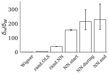
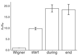
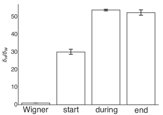
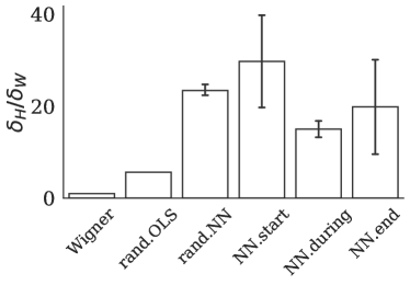
Empirical simulations suggest that this result holds already in small n๐‘›n settings (see Figureย 6) and finite n๐‘›n results can be likely derived under assumptions such as Gaussian data. As can be seen in Figureย 2 below, even for a practical batch size of n=32๐‘›32n=32 the diagonal mass ฮด๐‡subscript๐›ฟ๐‡\delta_{\bf H} of neural networks stays above both benchmarks for random inputs as well as with real-world data.
Refer to caption Refer to caption
โ€ƒSimple CNN (62k weights) โ€ƒMLP (411k weights)
Figure 2: Diagonal mass of neural network Hessian ฮด๐‡subscript๐›ฟ๐‡\delta_{\bf H} relative to ฮด๐”ผโ€‹[|๐–|]subscript๐›ฟ๐”ผdelimited-[]๐–\delta_{\mathbb{E}\left[|{\bf W}|\right]} and ฮด๐”ผโ€‹[|๐‡ols|]subscript๐›ฟ๐”ผdelimited-[]subscript๐‡ols\delta_{\mathbb{E}\left[|{\bf H}_{\text{ols}}|\right]} of corresponding dimensionality for random inputs as well as at random initialization, middle and after reaching 90%percent9090\% training accuracy with RMSProp on CIFAR-10. Mean and 95% confidence interval over 10 independent runs.

These results are in line with [6] and suggest that full matrix preconditioning might indeed not be worth the additional computational cost. Consequently, we use diagonal preconditioning for both first- and second-order methods in all of our experiments in Sectionย 5. Further theoretical elaborations of these findings present an interesting direction of future research.

4 Second-order Trust Region Methods

Cubic regularizationย [50, 14] and trust region methods belong to the family of globalized Newton methods. Both frameworks compute parameter updates by optimizing regularized (former) or constrained (latter) second-order Taylor models of the objective โ„’โ„’\mathcal{L} around the current iterate ๐ฐtsubscript๐ฐ๐‘ก{\bf w}_{t}.555In the following we only treat TR methods, but we emphasize that the use of matrix induced norms can directly be transferred to the cubic regularization framework. In particular, in iteration t๐‘กt the update step of the trust region algorithm is computed as

min๐ฌโˆˆโ„dโก[mtโ€‹(๐ฌ):=โ„’โ€‹(๐ฐt)+๐ tโŠบโ€‹๐ฌ+12โ€‹๐ฌโŠบโ€‹๐tโ€‹๐ฌ],s.t.โ€‹โ€–๐ฌโ€–๐€tโ‰คฮ”t,subscript๐ฌsuperscriptโ„๐‘‘assignsubscript๐‘š๐‘ก๐ฌโ„’subscript๐ฐ๐‘กsuperscriptsubscript๐ ๐‘กโŠบ๐ฌ12superscript๐ฌโŠบsubscript๐๐‘ก๐ฌs.t.subscriptnorm๐ฌsubscript๐€๐‘กsubscriptฮ”๐‘ก\displaystyle\min_{{\bf s}\in\mathbb{R}^{d}}\>\left[m_{t}({\bf s}):=\mathcal{L}({\bf w}_{t})+{\bf g}_{t}^{\intercal}{\bf s}+\frac{1}{2}{\bf s}^{\intercal}{\bf B}_{t}{\bf s}\right],\>\text{s.t.}\>\>\|{\bf s}\|_{{\bf A}_{t}}\leq\Delta_{t}, (7)

where ฮ”t>0subscriptฮ”๐‘ก0\Delta_{t}>0 and ๐ tsubscript๐ ๐‘ก{\bf g}_{t} and ๐tsubscript๐๐‘ก{\bf B}_{t} are either โˆ‡โ„’โ€‹(๐ฐt)โˆ‡โ„’subscript๐ฐ๐‘ก\nabla\mathcal{L}({\bf w}_{t}) and โˆ‡2โ„’โ€‹(๐ฐt)superscriptโˆ‡2โ„’subscript๐ฐ๐‘ก\nabla^{2}\mathcal{L}({\bf w}_{t}) or suitable approximations. The matrix ๐€tsubscript๐€๐‘ก{\bf A}_{t} induces the shape of the constraint set. So far, the common choice for neural networks is ๐€t:=๐ˆ,โˆ€tassignsubscript๐€๐‘ก๐ˆfor-all๐‘ก{\bf A}_{t}:=\mathbf{I},\;\forall t which gives rise to spherical trust regions [66, 42]. By solving the constrained problem (7), TR methods overcome the problem that pure Newton steps may be ascending, attracted by saddles or not even computable. Please see Appendix B for more details.

Why ellipsoids?

There are many sources for ill-conditioning in neural networks such as un-centered and correlated inputs [38], saturated hidden units, and different weight scales in different layersย [63]. While the quadratic term of model (7) accounts for such ill-conditioning to some extent, the spherical constraint is completely blind towards the loss surface. Thus, it is advisable to instead measure distances in norms that reflect the underlying geometry (see Chap. 7.7 in [19]). The ellipsoids we propose are such that they allow for longer steps along coordinates that have seen small gradient components in the past and vice versa. Thereby the TR shape is adaptively adjusted to fit the current region of the loss landscape. This is not only effective when the iterates are in an ill-conditioned neighborhood of a minimizer (Fig.ย 1), but it also helps to escape elongated plateaus (see autoencoder in Sec.ย 5). Contrary to adaptive first-order methods, the diameter (ฮ”tsubscriptฮ”๐‘ก\Delta_{t}) is updated directly depending on whether or not the local Taylor model is an adequate approximation at the current point.

4.1 Convergence of ellipsoidal Trust Region methods

Inspired by the success of adaptive gradient methods, we investigate the use of their preconditioning matrices as norm inducing matrices for second-order TR methods. The crucial condition for convergence is that the applied norms are not degenerate during the entire minimization process in the sense that the ellipsoids do not flatten out (or blow up) completely along any given direction. The following definition formalizes this intuition.

Definition 1 (Uniformly equivalent norms).

The norms โ€–๐ฐโ€–๐€t:=(๐ฐโŠบโ€‹๐€tโ€‹๐ฐ)1/2assignsubscriptnorm๐ฐsubscript๐€๐‘กsuperscriptsuperscript๐ฐโŠบsubscript๐€๐‘ก๐ฐ12\|{\bf w}\|_{{\bf A}_{t}}:=\left({\bf w}^{\intercal}{\bf A}_{t}{\bf w}\right)^{1/2} induced by symmetric positive definite matrices ๐€tsubscript๐€๐‘ก{\bf A}_{t} are called uniformly equivalent, if โˆƒฮผโ‰ฅ1๐œ‡1\exists\mu\geq 1 such that โˆ€๐ฐโˆˆโ„d,โˆ€t=1,2,โ€ฆformulae-sequencefor-all๐ฐsuperscriptโ„๐‘‘for-all๐‘ก12โ€ฆ\forall{\bf w}\in\mathbb{R}^{d},\forall t=1,2,\ldots

1ฮผโ€‹โ€–๐ฐโ€–๐€tโ‰คโ€–๐ฐโ€–2โ‰คฮผโ€‹โ€–๐ฐโ€–๐€t.1๐œ‡subscriptnorm๐ฐsubscript๐€๐‘กsubscriptnorm๐ฐ2๐œ‡subscriptnorm๐ฐsubscript๐€๐‘ก\displaystyle\frac{1}{\mu}\|{\bf w}\|_{{\bf A}_{t}}\leq\|{\bf w}\|_{2}\leq\mu\|{\bf w}\|_{{\bf A}_{t}}. (8)

We now establish a result which shows that the RMSProp ellipsoid is indeed uniformly equivalent.

Lemma 2 (Uniform equivalence).
Suppose โ€–๐ tโ€–2โ‰คLH2superscriptnormsubscript๐ ๐‘ก2superscriptsubscript๐ฟ๐ป2\|{\bf g}_{t}\|^{2}\leq L_{H}^{2} for all ๐ฐtโˆˆโ„d,subscript๐ฐ๐‘กsuperscriptโ„๐‘‘{\bf w}_{t}\in\mathbb{R}^{d}, t=1,2,โ€ฆ๐‘ก12โ€ฆt=1,2,\ldots Then there always exists ฯต>0italic-ฯต0\epsilon>0 such that the proposed preconditioning matrices ๐€rโ€‹mโ€‹s,tsubscript๐€๐‘Ÿ๐‘š๐‘ ๐‘ก{\bf A}_{rms,t} (Eq.ย 3) are uniformly equivalent, i.e. Def.ย 1 holds. The same holds for the diagonal variant.

Consequently, the ellipsoids ๐€rโ€‹mโ€‹s,tsubscript๐€๐‘Ÿ๐‘š๐‘ ๐‘ก{\bf A}_{rms,t} can directly be applied to any convergent TR framework without losing the guarantee of convergence ([19], Theorem 6.6.8).666Note that the assumption of bounded batch gradients, i.e. smooth objectives, is common in the analysis of stochastic algorithms [3, 24, 57, 27]. In Theorem 1 we extend this result by showing the (to the best of our knowledge) first convergence rate for ellipsoidal TR methods. Interestingly, similar results cannot be established for ๐€aโ€‹dโ€‹a,tsubscript๐€๐‘Ž๐‘‘๐‘Ž๐‘ก{\bf A}_{ada,t}, which reflects the widely known vanishing stepsize problem that arises since squared gradients are continuously added to the preconditioning matrix. At least partially, this effect inspired the development of RMSpropย [61] and Adadeltaย [69].

4.2 A stochastic ellipsoidal TR framework for neural network training

Since neural network training often constitutes a large-scale learning problem in which the number of datapoints n๐‘›n is high, we here opt for a stochastic TR framework in order to circumvent memory issues and reduce the computational complexity. To obtain convergence without computing full derivative information, we first need to assume sufficiently accurate gradient and Hessian estimates.

Assumption 1 (Sufficiently accurate derivatives).

The approximations of the gradient and Hessian at step t๐‘กt satisfy

โ€–๐ tโˆ’โˆ‡โ„’โ€‹(๐ฐt)โ€–โ‰คฮดgโ€‹ย andย โ€‹โ€–๐tโˆ’โˆ‡2โ„’โ€‹(๐ฐt)โ€–โ‰คฮดH,normsubscript๐ ๐‘กโˆ‡โ„’subscript๐ฐ๐‘กsubscript๐›ฟ๐‘”ย andย normsubscript๐๐‘กsuperscriptโˆ‡2โ„’subscript๐ฐ๐‘กsubscript๐›ฟ๐ป\displaystyle\|{\bf g}_{t}-\nabla\mathcal{L}({\bf w}_{t})\|\leq\delta_{g}\>\text{ and }\>\|{\bf B}_{t}-\nabla^{2}\mathcal{L}({\bf w}_{t})\|\leq\delta_{H},

where ฮดgโ‰ค(1โˆ’ฮท)โ€‹ฯตg4subscript๐›ฟ๐‘”1๐œ‚subscriptitalic-ฯต๐‘”4\delta_{g}\leq\frac{(1-\eta)\epsilon_{g}}{4} and ฮดHโ‰คminโก{(1โˆ’ฮท)โ€‹vโ€‹ฯตH2,1}subscript๐›ฟ๐ป1๐œ‚๐‘ฃsubscriptitalic-ฯต๐ป21\delta_{H}\leq\min\left\{\frac{(1-\eta)v\epsilon_{H}}{2},1\right\}, for some 0<v<10๐‘ฃ10<v<1.

For finite-sum objectives such as Eq.ย (1), the above condition can be met by random sub-sampling due to classical concentration results for sums of random variables [67, 37, 62]. Following these references, we assume access to the full function value in each iteration for our theoretical analysis but we note that convergence can be retained even for fully stochastic trust region methods [31, 18, 8] and indeed our experiments in Section 5 use sub-sampled function values due to memory constraints. Secondly, we adapt the framework of [68, 67], which allows for cheap inexact subproblem minimization, to the case of iteration-dependent constraint norms (Alg. 1).

Algorithm 1 Stochastic Ellipsoidal Trust Region Method
1:ย ย Input: ๐ฐ0โˆˆโ„dsubscript๐ฐ0superscriptโ„๐‘‘{\bf w}_{0}\in\mathbb{R}^{d}, ฮณ>1,1>ฮท>0formulae-sequence๐›พ11๐œ‚0\gamma>1,1>\eta>0, ฮ”0>0subscriptฮ”00\Delta_{0}>0
2:ย ย forย t=0,1,โ€ฆ,until convergence๐‘ก01โ€ฆuntil convergencet=0,1,\dots,\text{until convergence}ย do
3:ย ย ย ย ย Compute approximations ๐ tsubscript๐ ๐‘ก{\bf g}_{t} and ๐tsubscript๐๐‘ก{\bf B}_{t}.
4:ย ย ย ย ย If โ€–๐ tโ€–โ‰คฯตgnormsubscript๐ ๐‘กsubscriptitalic-ฯต๐‘”\|{\bf g}_{t}\|\leq\epsilon_{g}, set ๐ t:=0assignsubscript๐ ๐‘ก0{\bf g}_{t}:=0.
5:ย ย ย ย ย Set ๐€t:=๐€rโ€‹mโ€‹s,tassignsubscript๐€๐‘กsubscript๐€๐‘Ÿ๐‘š๐‘ ๐‘ก{\bf A}_{t}:={\bf A}_{rms,t} or ๐€t:=diagโ€‹(๐€rโ€‹mโ€‹s,t)assignsubscript๐€๐‘กdiagsubscript๐€๐‘Ÿ๐‘š๐‘ ๐‘ก{\bf A}_{t}:=\text{diag}\left({\bf A}_{rms,t}\right) (see Eq.ย (3)).
6:ย ย ย ย ย Obtain ๐ฌtsubscript๐ฌ๐‘ก{\bf s}_{t} by solving mtโ€‹(๐ฌt)subscript๐‘š๐‘กsubscript๐ฌ๐‘กm_{t}({\bf s}_{t}) approximately.
7:ย ย ย ย ย Compute ratio of function over model decrease: ฯt=โ„’โ€‹(๐ฐt)โˆ’โ„’โ€‹(๐ฐt+๐ฌt)mtโ€‹(๐ŸŽ)โˆ’mtโ€‹(๐ฌt)subscript๐œŒ๐‘กโ„’subscript๐ฐ๐‘กโ„’subscript๐ฐ๐‘กsubscript๐ฌ๐‘กsubscript๐‘š๐‘ก0subscript๐‘š๐‘กsubscript๐ฌ๐‘ก\>\rho_{t}=\dfrac{\mathcal{L}({\bf w}_{t})-\mathcal{L}({\bf w}_{t}+{\bf s}_{t})}{m_{t}({\bf 0})-m_{t}({\bf s}_{t})}
8:ย ย ย ย ย Set
ฮ”t+1subscriptฮ”๐‘ก1\displaystyle\Delta_{t+1} ={ฮณโ€‹ฮ”tย ifย โ€‹ฯ๐’ฎ,tโ‰ฅฮทฮ”t/ฮณย ifย โ€‹ฯ๐’ฎ,t<ฮท,|:ย andย ๐ฐt+1\displaystyle=\begin{cases}\gamma\Delta_{t}&\text{ if }\rho_{\mathcal{S},t}\geq\eta\\ \Delta_{t}/\gamma&\text{ if }\rho_{\mathcal{S},t}<\eta\end{cases},\>|:\text{ and }\>{\bf w}_{t+1} ={๐ฐt+๐ฌtย ifย โ€‹ฯtโ‰ฅฮทย (successful)๐ฐtย otherwiseย (unsuccessful).absentcasessubscript๐ฐ๐‘กsubscript๐ฌ๐‘กย ifย subscript๐œŒ๐‘ก๐œ‚ย (successful)subscript๐ฐ๐‘กย otherwiseย (unsuccessful).\displaystyle=\begin{cases}{\bf w}_{t}+{\bf s}_{t}&\text{ if }\rho_{t}\geq\eta\quad\;\text{ (successful)}\\ {\bf w}_{t}&\text{ otherwise}\quad\text{ (unsuccessful).}\end{cases}
9:ย ย endย for
Assumption 2 (Approximate model minimization).

Each update step ๐ฌtsubscript๐ฌ๐‘ก{\bf s}_{t} yields at least as much model decrease as the Cauchy- and Eigenpoint simultaneously, i.e.mtโ€‹(๐ฌt)โ‰คmtโ€‹(๐ฌtC)subscript๐‘š๐‘กsubscript๐ฌ๐‘กsubscript๐‘š๐‘กsuperscriptsubscript๐ฌ๐‘ก๐ถm_{t}({\bf s}_{t})\leq m_{t}({\bf s}_{t}^{C}) and mtโ€‹(๐ฌt)โ‰คmtโ€‹(๐ฌtE),subscript๐‘š๐‘กsubscript๐ฌ๐‘กsubscript๐‘š๐‘กsuperscriptsubscript๐ฌ๐‘ก๐ธm_{t}({\bf s}_{t})\leq m_{t}({\bf s}_{t}^{E}), where ๐ฌtCsuperscriptsubscript๐ฌ๐‘ก๐ถ{\bf s}_{t}^{C} and ๐ฌtEsuperscriptsubscript๐ฌ๐‘ก๐ธ{\bf s}_{t}^{E} are defined in Eq.(28).

Finally, given that the adaptive norms induced by ๐€rโ€‹mโ€‹s,tsubscript๐€๐‘Ÿ๐‘š๐‘ ๐‘ก{\bf A}_{rms,t} satisfy uniform equivalence as shown in Lemma 1, the following Theorem establishes an ๐’ชโ€‹(maxโ€‹{ฯตgโˆ’2โ€‹ฯตHโˆ’1,ฯตHโˆ’3})๐’ชmaxsuperscriptsubscriptitalic-ฯต๐‘”2superscriptsubscriptitalic-ฯต๐ป1superscriptsubscriptitalic-ฯต๐ป3{\cal O}\left(\text{max}\left\{\epsilon_{g}^{-2}\epsilon_{H}^{-1},\epsilon_{H}^{-3}\right\}\right) worst-case iteration complexity which effectively matches the one of [68].

Theorem 1 (Convergence rate of Algorithm 1).

Assume that โ„’โ€‹(๐ฐ)โ„’๐ฐ\mathcal{L({\bf w})} is second-order smooth with Lipschitz constants Lgsubscript๐ฟ๐‘”L_{g} and LHsubscript๐ฟ๐ปL_{H}. Furthermore, let Assumption 1 and 2 hold. Then Algorithm 1 finds an ๐’ชโ€‹(ฯตg,ฯตH)๐’ชsubscriptitalic-ฯต๐‘”subscriptitalic-ฯต๐ป\mathcal{O}(\epsilon_{g},\epsilon_{H}) first- and second-order stationary point in at most ๐’ชโ€‹(maxโก{ฯตgโˆ’2โ€‹ฯตHโˆ’1,ฯตHโˆ’3})๐’ชsuperscriptsubscriptitalic-ฯต๐‘”2superscriptsubscriptitalic-ฯต๐ป1superscriptsubscriptitalic-ฯต๐ป3\mathcal{O}\left(\max\left\{\epsilon_{g}^{-2}\epsilon_{H}^{-1},\epsilon_{H}^{-3}\right\}\right) iterations.

ResNet18 MLP Autoencoder

Fashion-MNIST

Refer to caption Refer to caption Refer to caption

CIFAR-10

Refer to caption Refer to caption Refer to caption
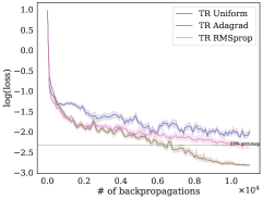
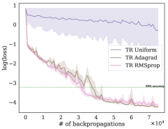
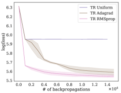
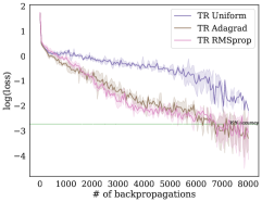
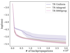
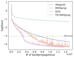
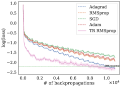
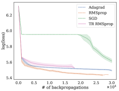
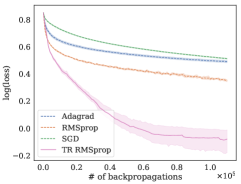
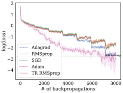
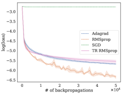
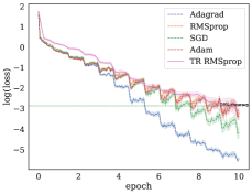
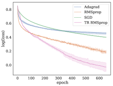
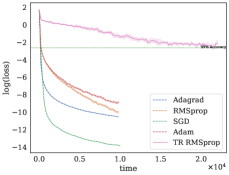
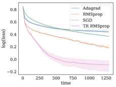
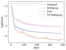
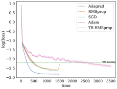
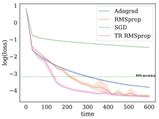
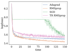
Figure 3: Log loss over backpropagations. Mean and 95%percent9595\% confidence interval of 10 runs. Green dotted line indicates 99%percent9999\% training accuracy.

The proof of this statement is a straight-forward adaption of the proof for spherical constraints, taking into account that the guaranteed model decrease changes when the computed step stsubscript๐‘ ๐‘กs_{t} lies outside the Trust Region. Due to the uniform equivalence established in 1, the altered diameter of the trust region along that direction and hence the change factor is always strictly positive and finite.

5 Experiments

To validate our claim that ellipsoidal TR methods yield improved performance over spherical ones, we run a set of experiments on two image datasets and three types of network architectures. All methods run on (almost) the same hyperparameters across all experiments (see Table 1 in Appendix B) and employ the preconditionied Steihaug-Toint CG method [60] to solve the subproblems (Eq.ย 50) with the classical stopping criterion given in Eq.ย (52).

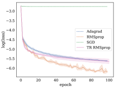
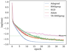
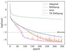
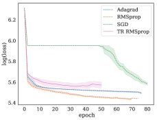
As depicted in Fig.ย 3, the ellipsoidal TR methods consistently outperform their spherical counterpart in the sense that they reach full training accuracy substantially faster on all problems. Moreover, their limit points are in all cases lower than those of the uniform method. Interestingly, this makes an actual difference in the image reconstruction quality of autoencoders (see Figureย 12), where the spherically constrained TR method struggles to escape a saddle. We thus draw the clear conclusion that the ellipsoidal constraints we propose are to be preferred over spherical ones when training neural nets with second-order methods. More experimental and architectural details are provided in App. C.

To put the previous results into context, we also benchmark several state-of-the-art gradient methods. For a fair comparison, we report results in terms of number of backpropagations, epochs and time. All figures can be found in App. C. Our findings are mixed: For small nets such as the MLPs the TR method with RMSProp ellipsoids is superior in all metrics, even when benchmarked in terms of time. However, while Fig. 9 indicates that ellipsoidal TR methods are slightly superior in terms of backpropagations even for ResNets and Autoencoders, a close look at the Figures 10 and 11 (App. C) reveals that they at best manage to keep pace with first-order methods in terms of epochs and are inferior in time. Furthermore, only the autoencoders give rise to saddles, which adaptive gradient methods escape faster than vanilla SGD, similarly to the case for second-order methods in Fig. 3.

6 Conclusion

We investigated the use of ellipsoidal trust region constraints for neural networks. We have shown that the RMSProp matrix satisfies the necessary conditions for convergence and our experimental results demonstrate that ellipsoidal TR methods outperform their spherical counterparts significantly. We thus consider the development of further ellipsoids that can potentially adapt even better to the loss landscape such as e.g. (block-) diagonal hessian approximations (e.g.ย [7]) or approximations of higher order derivatives as an interesting direction of future research.

Yet, the gradient method benchmark indicates that the value of Hessian information for neural network training is limited for mainly three reasons: 1) second-order methods rarely yield better limit points, which suggests that saddles and spurious local minima are not a major obstacle; 2) gradient methods can run on smaller batch sizes which is beneficial in terms of epoch and when memory is limited; 3) The per-iteration time complexity is noticeably lower for first-order methods (Figure 11). These observations suggest that advances in hardware and distributed second-order algorithms (e.g., ย [52, 28]) will be needed before Newton-type methods can replace gradient methods in deep learning.

As a side note, we reported elevated levels of diagonal dominance in neural network architectures, which may partially explain the success of diagonal preconditioning in first-order method. Further empirical and theoretical investigations of this phenomenon with a particular focus on layer-wise dependencies constitute an interesting direction of future research as for example algorithms such as K-FAC [32] seem to achieve good results with block-diagonal preconditioning.

Broader impact

We consider our work fundamental research with no specific application other than training neural networks in general. Hence a broader impact discussion is not applicable.

References

  • [1] Naman Agarwal, Brian Bullins, Xinyi Chen, Elad Hazan, Karan Singh, Cyril Zhang, and Yiย Zhang. The case for full-matrix adaptive regularization. arXiv preprint arXiv:1806.02958, 2018.
  • [2] Guillaume Alain, Nicolas Leย Roux, and Pierre-Antoine Manzagol. Negative eigenvalues of the hessian in deep neural networks. 2018.
  • [3] Zeyuan Allen-Zhu. Katyusha: The first direct acceleration of stochastic gradient methods. The Journal of Machine Learning Research, 18(1):8194โ€“8244, 2017.
  • [4] Zeyuan Allen-Zhu, Yuanzhi Li, and Zhao Song. A convergence theory for deep learning via over-parameterization. arXiv preprint arXiv:1811.03962, 2018.
  • [5] Shun-Ichi Amari. Natural gradient works efficiently in learning. Neural computation, 10(2):251โ€“276, 1998.
  • [6] Sue Becker, Yann Leย Cun, etย al. Improving the convergence of back-propagation learning with second order methods. In Proceedings of the 1988 connectionist models summer school, pages 29โ€“37. San Matteo, CA: Morgan Kaufmann, 1988.
  • [7] Costas Bekas, Effrosyni Kokiopoulou, and Yousef Saad. An estimator for the diagonal of a matrix. Applied numerical mathematics, 57(11-12):1214โ€“1229, 2007.
  • [8] Jose Blanchet, Coralia Cartis, Matt Menickelly, and Katya Scheinberg. Convergence rate analysis of a stochastic trust region method for nonconvex optimization. arXiv preprint arXiv:1609.07428, 2016.
  • [9] Leon Bottou. Large-scale machine learning with stochastic gradient descent. In Proceedings of COMPSTATโ€™2010, pages 177โ€“186. Springer, 2010.
  • [10] Lรฉon Bottou, Frankย E Curtis, and Jorge Nocedal. Optimization methods for large-scale machine learning. SIAM Review, 60(2):223โ€“311, 2018.
  • [11] Alon Brutzkus and Amir Globerson. Globally optimal gradient descent for a convnet with gaussian inputs. arXiv preprint arXiv:1702.07966, 2017.
  • [12] Yair Carmon, Johnย C Duchi, Oliver Hinder, and Aaron Sidford. Lower bounds for finding stationary points i. arXiv preprint arXiv:1710.11606, 2017.
  • [13] Coralia Cartis, Nicholasย IM Gould, and Phย L Toint. Complexity bounds for second-order optimality in unconstrained optimization. Journal of Complexity, 28(1):93โ€“108, 2012.
  • [14] Coralia Cartis, Nicholasย IM Gould, and Philippeย L Toint. Adaptive cubic regularisation methods for unconstrained optimization. part i: motivation, convergence and numerical results. Mathematical Programming, 127(2):245โ€“295, 2011.
  • [15] Coralia Cartis, Nicholasย IM Gould, and Philippeย L Toint. How Much Patience to You Have?: A Worst-case Perspective on Smooth Noncovex Optimization. Science and Technology Facilities Council Swindon, 2012.
  • [16] Coralia Cartis and Katya Scheinberg. Global convergence rate analysis of unconstrained optimization methods based on probabilistic models. Mathematical Programming, pages 1โ€“39, 2017.
  • [17] Olivier Chapelle and Dumitru Erhan. Improved preconditioner for hessian free optimization. In NIPS Workshop on Deep Learning and Unsupervised Feature Learning, volume 201, 2011.
  • [18] Ruobing Chen, Matt Menickelly, and Katya Scheinberg. Stochastic optimization using a trust-region method and random models. Mathematical Programming, 169(2):447โ€“487, 2018.
  • [19] Andrewย R Conn, Nicholasย IM Gould, and Philippeย L Toint. Trust region methods. SIAM, 2000.
  • [20] Frankย E Curtis and Danielย P Robinson. Exploiting negative curvature in deterministic and stochastic optimization. arXiv preprint arXiv:1703.00412, 2017.
  • [21] Frankย E Curtis, Danielย P Robinson, and Mohammadreza Samadi. A trust region algorithm with a worst-case iteration complexity of ๐’ชโ€‹(ฯต3โˆ’2)๐’ชsuperscriptitalic-ฯต32\mathcal{O}(\epsilon^{3-2}) for nonconvex optimization. Mathematical Programming, 162(1-2):1โ€“32, 2017.
  • [22] Hadi Daneshmand, Jonas Kohler, Aurelien Lucchi, and Thomas Hofmann. Escaping saddles with stochastic gradients. arXiv preprint arXiv:1803.05999, 2018.
  • [23] Yannย N Dauphin, Razvan Pascanu, Caglar Gulcehre, Kyunghyun Cho, Surya Ganguli, and Yoshua Bengio. Identifying and attacking the saddle point problem in high-dimensional non-convex optimization. In Advances in neural information processing systems, pages 2933โ€“2941, 2014.
  • [24] Aaron Defazio, Francis Bach, and Simon Lacoste-Julien. Saga: A fast incremental gradient method with support for non-strongly convex composite objectives. In Advances in neural information processing systems, pages 1646โ€“1654, 2014.
  • [25] Simonย S Du, Chi Jin, Jasonย D Lee, Michaelย I Jordan, Aarti Singh, and Barnabas Poczos. Gradient descent can take exponential time to escape saddle points. In Advances in Neural Information Processing Systems, pages 1067โ€“1077, 2017.
  • [26] Simonย S Du and Jasonย D Lee. On the power of over-parametrization in neural networks with quadratic activation. arXiv preprint arXiv:1803.01206, 2018.
  • [27] John Duchi, Elad Hazan, and Yoram Singer. Adaptive subgradient methods for online learning and stochastic optimization. Journal of Machine Learning Research, 12(Jul):2121โ€“2159, 2011.
  • [28] Celestine Dรผnner, Aurelien Lucchi, Matilde Gargiani, Anย Bian, Thomas Hofmann, and Martin Jaggi. A distributed second-order algorithm you can trust. arXiv preprint arXiv:1806.07569, 2018.
  • [29] Rong Ge, Furong Huang, Chi Jin, and Yang Yuan. Escaping from saddle points-online stochastic gradient for tensor decomposition. In COLT, pages 797โ€“842, 2015.
  • [30] Gabriel Goh. Why momentum really works. Distill, 2017.
  • [31] Serge Gratton, Clรฉmentย W Royer, Luรญsย N Vicente, and Zaikun Zhang. Complexity and global rates of trust-region methods based on probabilistic models. IMA Journal of Numerical Analysis, 2017.
  • [32] Roger Grosse and James Martens. A kronecker-factored approximate fisher matrix for convolution layers. In International Conference on Machine Learning, pages 573โ€“582, 2016.
  • [33] Martinย T Hagan and Mohammadย B Menhaj. Training feedforward networks with the marquardt algorithm. IEEE transactions on Neural Networks, 5(6):989โ€“993, 1994.
  • [34] Geoffreyย E Hinton and Ruslanย R Salakhutdinov. Reducing the dimensionality of data with neural networks. science, 313(5786):504โ€“507, 2006.
  • [35] Stanislaw Jastrzebski, Zachary Kenton, Devansh Arpit, Nicolas Ballas, Asja Fischer, Yoshua Bengio, and Amos Storkey. Three factors influencing minima in sgd. arXiv preprint arXiv:1711.04623, 2017.
  • [36] Diederikย P Kingma and Jimmy Ba. Adam: A method for stochastic optimization. arXiv preprint arXiv:1412.6980, 2014.
  • [37] Jonasย Moritz Kohler and Aurelien Lucchi. Sub-sampled cubic regularization for non-convex optimization. In International Conference on Machine Learning, 2017.
  • [38] Yannย A LeCun, Lรฉon Bottou, Genevieveย B Orr, and Klaus-Robert Mรผller. Efficient backprop. In Neural networks: Tricks of the trade, pages 9โ€“48. Springer, 2012.
  • [39] Jasonย D Lee, Max Simchowitz, Michaelย I Jordan, and Benjamin Recht. Gradient descent only converges to minimizers. In Conference on Learning Theory, pages 1246โ€“1257, 2016.
  • [40] Xiaoyu Li and Francesco Orabona. On the convergence of stochastic gradient descent with adaptive stepsizes. arXiv preprint arXiv:1805.08114, 2018.
  • [41] Yuanzhi Li and Yang Yuan. Convergence analysis of two-layer neural networks with relu activation. In Advances in Neural Information Processing Systems, pages 597โ€“607, 2017.
  • [42] Liu Liu, Xuanqing Liu, Cho-Jui Hsieh, and Dacheng Tao. Stochastic second-order methods for non-convex optimization with inexact hessian and gradient. arXiv preprint arXiv:1809.09853, 2018.
  • [43] Linjian Ma, Gabe Montague, Jiayu Ye, Zhewei Yao, Amir Gholami, Kurt Keutzer, and Michaelย W Mahoney. Inefficiency of k-fac for large batch size training. arXiv preprint arXiv:1903.06237, 2019.
  • [44] James Martens. Deep learning via hessian-free optimization. In ICML, volumeย 27, pages 735โ€“742, 2010.
  • [45] James Martens. New insights and perspectives on the natural gradient method. arXiv preprint arXiv:1412.1193, 2014.
  • [46] James Martens and Roger Grosse. Optimizing neural networks with kronecker-factored approximate curvature. In International conference on machine learning, pages 2408โ€“2417, 2015.
  • [47] Dominic Masters and Carlo Luschi. Revisiting small batch training for deep neural networks. arXiv preprint arXiv:1804.07612, 2018.
  • [48] Eiji Mizutani and Stuartย E Dreyfus. Second-order stagewise backpropagation for hessian-matrix analyses and investigation of negative curvature. Neural Networks, 21(2-3):193โ€“203, 2008.
  • [49] Yurii Nesterov. Introductory lectures on convex optimization: A basic course, volumeย 87. Springer Science & Business Media, 2013.
  • [50] Yurii Nesterov and Borisย T Polyak. Cubic regularization of newton method and its global performance. Mathematical Programming, 108(1):177โ€“205, 2006.
  • [51] Jorge Nocedal and Stephenย J Wright. Numerical optimization, 2nd Edition. Springer, 2006.
  • [52] Kazuki Osawa, Yohei Tsuji, Yuichiro Ueno, Akira Naruse, Rio Yokota, and Satoshi Matsuoka. Second-order optimization method for large mini-batch: Training resnet-50 on imagenet in 35 epochs. arXiv preprint arXiv:1811.12019, 2018.
  • [53] Razvan Pascanu and Yoshua Bengio. Revisiting natural gradient for deep networks. arXiv preprint arXiv:1301.3584, 2013.
  • [54] Adam Paszke, Sam Gross, Soumith Chintala, Gregory Chanan, Edward Yang, Zachary DeVito, Zeming Lin, Luca Desmaison, Alban aComplexity bounds for second-order optimality in unconstrained optimizationndย Antiga, and Adam Lerer. Automatic differentiation in pytorch. 2017.
  • [55] Barakย A Pearlmutter. Fast exact multiplication by the hessian. Neural computation, 6(1):147โ€“160, 1994.
  • [56] Herbert Robbins and Sutton Monro. A stochastic approximation method. In The Annals of Mathematical Statistics - Volume 22, Number 3. Institute of Mathematical Statistics, 1951.
  • [57] Mark Schmidt, Nicolas Leย Roux, and Francis Bach. Minimizing finite sums with the stochastic average gradient. Mathematical Programming, 162(1-2):83โ€“112, 2017.
  • [58] Nicolย N Schraudolph. Fast curvature matrix-vector products for second-order gradient descent. Neural computation, 14(7):1723โ€“1738, 2002.
  • [59] Shai Shalev-Shwartz, Ohad Shamir, and Shaked Shammah. Failures of gradient-based deep learning. arXiv preprint arXiv:1703.07950, 2017.
  • [60] Trond Steihaug. The conjugate gradient method and trust regions in large scale optimization. SIAM Journal on Numerical Analysis, 20(3):626โ€“637, 1983.
  • [61] Tijmen Tieleman and Geoffrey Hinton. Lecture 6.5-rmsprop: Divide the gradient by a running average of its recent magnitude. COURSERA: Neural networks for machine learning, 4(2):26โ€“31, 2012.
  • [62] Nilesh Tripuraneni, Mitchell Stern, Chi Jin, Jeffrey Regier, and Michaelย I Jordan. Stochastic cubic regularization for fast nonconvex optimization. arXiv preprint arXiv:1711.02838, 2017.
  • [63] Patrick Van Derย Smagt and Gerd Hirzinger. Solving the ill-conditioning in neural network learning. In Neural networks: tricks of the trade, pages 193โ€“206. Springer, 1998.
  • [64] Rachel Ward, Xiaoxia Wu, and Leon Bottou. Adagrad stepsizes: Sharp convergence over nonconvex landscapes, from any initialization. arXiv preprint arXiv:1806.01811, 2018.
  • [65] Eugeneย P Wigner. Characteristic vectors of bordered matrices with infinite dimensions i. In The Collected Works of Eugene Paul Wigner, pages 524โ€“540. Springer, 1993.
  • [66] Peng Xu, Farbod Roosta-Khorasan, and Michaelย W Mahoney. Second-order optimization for non-convex machine learning: An empirical study. arXiv preprint arXiv:1708.07827, 2017.
  • [67] Peng Xu, Farbod Roosta-Khorasani, and Michaelย W Mahoney. Newton-type methods for non-convex optimization under inexact hessian information. arXiv preprint arXiv:1708.07164, 2017.
  • [68] Zhewei Yao, Peng Xu, Farbod Roosta-Khorasani, and Michaelย W Mahoney. Inexact non-convex newton-type methods. arXiv preprint arXiv:1802.06925, 2018.
  • [69] Matthewย D Zeiler. Adadelta: an adaptive learning rate method. arXiv preprint arXiv:1212.5701, 2012.

Appendix A: Proofs

Appendix A Notation

Throughout this work, scalars are denoted by regular lower case letters, vectors by bold lower case letters and matrices as well as tensors by bold upper case letters. By โˆฅโ‹…โˆฅ\|\cdot\| we denote an arbitrary norm. For a symmetric positive definite matrix ๐€๐€{\bf A} we introduce the compact notation โ€–๐ฐโ€–๐€=(๐ฐโŠบโ€‹๐€๐ฐ)1/2subscriptnorm๐ฐ๐€superscriptsuperscript๐ฐโŠบ๐€๐ฐ12\|{\bf w}\|_{\bf A}=\left({\bf w}^{\intercal}{\bf A}{\bf w}\right)^{1/2}, where ๐ฐโˆˆโ„d๐ฐsuperscriptโ„๐‘‘{\bf w}\in\mathbb{R}^{d}.

Appendix B Equivalence of Preconditioned Gradient Descent and first-order Trust Region Methods

Theorem 2 (Theorem 1 restated).
A preconditioned gradient step ๐ฐt+1โˆ’๐ฐt=๐ฌt:=โˆ’ฮทtโ€‹๐€tโˆ’1โ€‹๐ tsubscript๐ฐ๐‘ก1subscript๐ฐ๐‘กsubscript๐ฌ๐‘กassignsubscript๐œ‚๐‘กsuperscriptsubscript๐€๐‘ก1subscript๐ ๐‘ก{\bf w}_{t+1}-{\bf w}_{t}={\bf s}_{t}:=-\eta_{t}{\bf A}_{t}^{-1}{\bf g}_{t} (9) with stepsize ฮทt>0subscript๐œ‚๐‘ก0\eta_{t}>0, symmetric positive definite preconditioner ๐€tโˆˆโ„dร—dsubscript๐€๐‘กsuperscriptโ„๐‘‘๐‘‘{\bf A}_{t}\in\mathbb{R}^{d\times d} and ๐ tโ‰ 0subscript๐ ๐‘ก0{\bf g}_{t}\not=0 minimizes a first-order local model around ๐ฐtโˆˆโ„subscript๐ฐ๐‘กโ„{\bf w}_{t}\in\mathbb{R} in an ellipsoid given by ๐€tsubscript๐€๐‘ก{\bf A}_{t} in the sense that ๐ฌt:=assignsubscript๐ฌ๐‘กabsent\displaystyle{\bf s}_{t}:= argโกmin๐ฌโˆˆโ„dโก[mt1โ€‹(๐ฌ)=โ„’โ€‹(๐ฐt)+๐ฌโŠบโ€‹๐ t],s.t.โ€‹โ€–๐ฌโ€–๐€tโ‰คฮทtโ€‹โ€–๐ tโ€–๐€tโˆ’1.subscript๐ฌsuperscriptโ„๐‘‘superscriptsubscript๐‘š๐‘ก1๐ฌโ„’subscript๐ฐ๐‘กsuperscript๐ฌโŠบsubscript๐ ๐‘กs.t.subscriptnorm๐ฌsubscript๐€๐‘กsubscript๐œ‚๐‘กsubscriptnormsubscript๐ ๐‘กsuperscriptsubscript๐€๐‘ก1\displaystyle\arg\min_{{\bf s}\in\mathbb{R}^{d}}\left[m_{t}^{1}({\bf s})=\mathcal{L}({\bf w}_{t})+{\bf s}^{\intercal}{\bf g}_{t}\right],\quad\text{s.t.}\;\|{\bf s}\|_{{\bf A}_{t}}\leq\eta_{t}\|{\bf g}_{t}\|_{{\bf A}_{t}^{-1}}. (10)
Proof.

We start the proof by noting that the optimization problem in Eq. (10) is convex. For ฮทt>0subscript๐œ‚๐‘ก0\eta_{t}>0 the constraint satisfies the Slater condition since 00 is a strictly feasible point. As a result, any KKT point is a feasible minimizer and vice versa.

Let Lโ€‹(๐ฌ,ฮป)๐ฟ๐ฌ๐œ†L({\bf s},\lambda) denote the Lagrange dual of Eq.ย (5)

Lโ€‹(๐ฌ,ฮป):=โ„’โ€‹(๐ฐt)+๐ฌโŠบโ€‹๐ t+ฮปโ€‹(โ€–๐ฌโ€–๐€โˆ’ฮทtโ€‹โ€–๐ tโ€–๐€tโˆ’1).assign๐ฟ๐ฌ๐œ†โ„’subscript๐ฐ๐‘กsuperscript๐ฌโŠบsubscript๐ ๐‘ก๐œ†subscriptnorm๐ฌ๐€subscript๐œ‚๐‘กsubscriptnormsubscript๐ ๐‘กsuperscriptsubscript๐€๐‘ก1L({\bf s},\lambda):=\mathcal{L}({\bf w}_{t})+{\bf s}^{\intercal}{\bf g}_{t}+\lambda\left(\|{\bf s}\|_{\bf A}-\eta_{t}\|{\bf g}_{t}\|_{{\bf A}_{t}^{-1}}\right). (11)

Any point ๐ฌ๐ฌ{\bf s} is a KKT point if and only if the following system of equations is satisfied

โˆ‡๐ฌLโ€‹(๐ฌ,ฮป)=๐ t+ฮปโ€–๐ฌโ€–๐€tโ€‹๐€tโ€‹๐ฌ=0subscriptโˆ‡๐ฌ๐ฟ๐ฌ๐œ†subscript๐ ๐‘ก๐œ†subscriptnorm๐ฌsubscript๐€๐‘กsubscript๐€๐‘ก๐ฌ0\displaystyle\nabla_{{\bf s}}L({\bf s},\lambda)={\bf g}_{t}+\frac{\lambda}{\|{\bf s}\|_{{\bf A}_{t}}}{\bf A}_{t}{\bf s}=0 (12)
ฮปโ€‹(โ€–๐ฌโ€–๐€tโˆ’ฮทtโ€‹โ€–๐ tโ€–๐€tโˆ’1)=0.๐œ†subscriptnorm๐ฌsubscript๐€๐‘กsubscript๐œ‚๐‘กsubscriptnormsubscript๐ ๐‘กsuperscriptsubscript๐€๐‘ก10\displaystyle\lambda\left(\|{\bf s}\|_{{\bf A}_{t}}-\eta_{t}\|{\bf g}_{t}\|_{{\bf A}_{t}^{-1}}\right)=0. (13)
โ€–๐ฌโ€–๐€tโˆ’ฮทtโ€‹โ€–๐ tโ€–๐€tโˆ’1โ‰ค0subscriptnorm๐ฌsubscript๐€๐‘กsubscript๐œ‚๐‘กsubscriptnormsubscript๐ ๐‘กsuperscriptsubscript๐€๐‘ก10\displaystyle\|{\bf s}\|_{{\bf A}_{t}}-\eta_{t}\|{\bf g}_{t}\|_{{\bf A}_{t}^{-1}}\leq 0 (14)
ฮปโ‰ฅ0.๐œ†0\displaystyle\lambda\geq 0. (15)

For ๐ฌtsubscript๐ฌ๐‘ก{\bf s}_{t} as given in Eq. (4) we have that

โ€–๐ฌtโ€–๐€t=ฮทt2โ€‹๐ tโ€‹(๐€tโˆ’1)โŠบโ€‹๐€tโ€‹๐€tโˆ’1โ€‹๐ t=ฮทtโ€‹๐ tโ€‹๐€tโˆ’1โ€‹๐ t=ฮทtโ€‹โ€–๐ tโ€–๐€tโˆ’1.subscriptnormsubscript๐ฌ๐‘กsubscript๐€๐‘กsuperscriptsubscript๐œ‚๐‘ก2subscript๐ ๐‘กsuperscriptsuperscriptsubscript๐€๐‘ก1โŠบsubscript๐€๐‘กsuperscriptsubscript๐€๐‘ก1subscript๐ ๐‘กsubscript๐œ‚๐‘กsubscript๐ ๐‘กsuperscriptsubscript๐€๐‘ก1subscript๐ ๐‘กsubscript๐œ‚๐‘กsubscriptnormsubscript๐ ๐‘กsuperscriptsubscript๐€๐‘ก1\|{\bf s}_{t}\|_{{\bf A}_{t}}=\sqrt{\eta_{t}^{2}{\bf g}_{t}{({\bf A}_{t}^{-1})}^{\intercal}{\bf A}_{t}{\bf A}_{t}^{-1}{\bf g}_{t}}=\eta_{t}\sqrt{{\bf g}_{t}{\bf A}_{t}^{-1}{\bf g}_{t}}=\eta_{t}\|{\bf g}_{t}\|_{{\bf A}_{t}^{-1}}. (16)

and thus 13 and 14 hold with equality such that any ฮปโ‰ฅ0๐œ†0\lambda\geq 0 is feasible. Furthermore,

โˆ‡๐ฌLโ€‹(๐ฌt,ฮป)subscriptโˆ‡๐ฌ๐ฟsubscript๐ฌ๐‘ก๐œ†\displaystyle\nabla_{{\bf s}}L({\bf s}_{t},\lambda) =โˆ‡fโ€‹(๐ฐt)+ฮปโ€–๐ฌtโ€–๐€tโ€‹๐€tโ€‹๐ฌtabsentโˆ‡๐‘“subscript๐ฐ๐‘ก๐œ†subscriptnormsubscript๐ฌ๐‘กsubscript๐€๐‘กsubscript๐€๐‘กsubscript๐ฌ๐‘ก\displaystyle=\nabla f({\bf w}_{t})+\frac{\lambda}{\|{\bf s}_{t}\|_{{\bf A}_{t}}}{\bf A}_{t}{\bf s}_{t} =(4)โ€‹๐ tโˆ’ฮทtโ€‹ฮปฮทtโ€‹โ€–๐ tโ€–๐€tโˆ’1โ€‹๐€tโ€‹๐€tโˆ’1โ€‹๐ t4subscript๐ ๐‘กsubscript๐œ‚๐‘ก๐œ†subscript๐œ‚๐‘กsubscriptnormsubscript๐ ๐‘กsuperscriptsubscript๐€๐‘ก1subscript๐€๐‘กsuperscriptsubscript๐€๐‘ก1subscript๐ ๐‘ก\displaystyle\overset{(\ref{eq:precond_gd_step})}{=}{\bf g}_{t}-\eta_{t}\frac{\lambda}{\eta_{t}\|{\bf g}_{t}\|_{{\bf A}_{t}^{-1}}}{\bf A}_{t}{\bf A}_{t}^{-1}{\bf g}_{t} =๐ tโˆ’ฮปโ€–๐ tโ€–๐€tโˆ’1โ€‹๐ tabsentsubscript๐ ๐‘ก๐œ†subscriptnormsubscript๐ ๐‘กsuperscriptsubscript๐€๐‘ก1subscript๐ ๐‘ก\displaystyle={\bf g}_{t}-\frac{\lambda}{\|{\bf g}_{t}\|_{{\bf A}_{t}^{-1}}}{\bf g}_{t} (17)

is zero for ฮป=โ€–๐ tโ€–๐€โˆ’1โ‰ฅ0๐œ†subscriptnormsubscript๐ ๐‘กsuperscript๐€10\lambda=\|{\bf g}_{t}\|_{{\bf A}^{-1}}\geq 0. As a result, ๐ฌtsubscript๐ฌ๐‘ก{\bf s}_{t} is a KKT point of the convex problem 5 which proves the assertion.

โˆŽ

To illustrate this theoretical result we run gradient descent and Adagrad as well as the two corresponding first-order TR methods777Essentially Algorithm 1 with mtsubscript๐‘š๐‘กm_{t} based on a first order Taylor expansion, i.e. mt1โ€‹(๐ฌ)superscriptsubscript๐‘š๐‘ก1๐ฌm_{t}^{1}({\bf s}) as in Eq.ย (10). on an ill-conditioned quadratic problem. While the method 1st TR optimizes a linear model within a ball in each iteration, 1st TRadaada{}_{\text{ada}} optimizes the same model over the ellipsoid given by the Adagrad matrix ๐€aโ€‹dโ€‹asubscript๐€๐‘Ž๐‘‘๐‘Ž{\bf A}_{ada}. The results in Figure 4 show that the methods behave very similarly to their constant stepsize analogues.

Figure 4: Iterates (left) and log suboptimality (right) of GD, Adagrad and two full-featured first-order TR algorithms of which one (1st TR) is spherically constraint and the other (1st TRadaada{}_{\text{ada}}) uses ๐€aโ€‹dโ€‹asubscript๐€๐‘Ž๐‘‘๐‘Ž{\bf A}_{ada} as ellispoid.

Appendix C Convergence of ellipsoidal TR methods

C.1 Proof sketch

At a high level, the proof can be divided into two steps: 1) establish that each update decreases the model value and 2) relate the model decrease to the function decrease, therefore proving that the function decreases.

Based on Assumption 2 the proof first relates the model decrease in each iteration to the gradient norm โ€–๐ tโ€–normsubscript๐ ๐‘ก\|{\bf g}_{t}\| and the magnitude of the smallest eigenvalue |ฮปminโ€‹(โ„ฌt)|subscript๐œ†subscriptโ„ฌ๐‘ก|\lambda_{\min}({\mathcal{B}}_{t})| as well as ฮ”tsubscriptฮ”๐‘ก\Delta_{t}. In the case of interior solutions (โ€–๐ฌtโ€–t<ฮ”subscriptnormsubscript๐ฌ๐‘ก๐‘กฮ”\|{\bf s}_{t}\|_{t}<\Delta), nothing changes compared to spherical Trust Region methods. When the computed step stsubscript๐‘ ๐‘กs_{t} lies outside the Trust Region, however, the guaranteed model decrease changes by a constant factor, which accounts for the altered diameter of the trust region along that direction. Due to the uniform equivalence established in 1 this factor is always strictly positive and finite.

More specifically, the first step of the proof relies on Assumption 2 in order to relate the model decrease at each iteration t๐‘กt to three quantities of interest: i) the gradient norm โ€–๐ tโ€–normsubscript๐ ๐‘ก\|{\bf g}_{t}\|, ii) the magnitude of the smallest eigenvalue |ฮปminโ€‹(โ„ฌt)|subscript๐œ†subscriptโ„ฌ๐‘ก|\lambda_{\min}({\mathcal{B}}_{t})|, and iii) the trust region radius ฮ”tsubscriptฮ”๐‘ก\Delta_{t}. In the case of interior solutions (โ€–๐ฌtโ€–t<ฮ”subscriptnormsubscript๐ฌ๐‘ก๐‘กฮ”\|{\bf s}_{t}\|_{t}<\Delta), the model decrease is shown as in the spherical Trust Region methods. When the computed step stsubscript๐‘ ๐‘กs_{t} lies outside the Trust Region, however, the guaranteed model decrease changes by a constant factor, which accounts for the altered diameter of the trust region along that direction. Due to the uniform equivalence established in Lemma 2 this factor is always strictly positive and finite.

From here on, the proof proceeds in a standard fashion (see e.g. [68]). That is, a lower bound on ฮ”tsubscriptฮ”๐‘ก\Delta_{t} is established which (i) upper bounds the number of unsuccessful steps and (ii) lower bounds the guaranteed model decrease introduced above, which in turn allows to bound the overall number of successful steps as a fraction of the initial suboptimality in โ„’โ„’\mathcal{L}. Assumption 1 together with the smoothness assumptions on โ„’โ„’\mathcal{L} allow to finally relate the progress of each successful step to the actual function decrease. Finally, since the function decreases and because it is lower bounded, there is a finite number of steps which we can upper bound.

C.2 Proof

In order to prove convergence results for ellipsoidal Trust Region methods one must ensure that the applied norms are coherent during the complete minimization process in the sense that the ellipsoids do not flatten out (or blow up) completely along any given direction. This intuition is formalized in Assumption 1 which we restate here for the sake of clarity.

Definition 2 (Definition 1 restated).

There exists a constant ฮผโ‰ฅ1๐œ‡1\mu\geq 1 such that

1ฮผโ€‹โ€–๐ฐโ€–๐€tโ‰คโ€–๐ฐโ€–2โ‰คฮผโ€‹โ€–๐ฐโ€–๐€t,โˆ€t,โˆ€๐ฐโˆˆโ„d.formulae-sequence1๐œ‡subscriptnorm๐ฐsubscript๐€๐‘กsubscriptnorm๐ฐ2๐œ‡subscriptnorm๐ฐsubscript๐€๐‘กfor-all๐‘กfor-all๐ฐsuperscriptโ„๐‘‘\frac{1}{\mu}\|{\bf w}\|_{{\bf A}_{t}}\leq\|{\bf w}\|_{2}\leq\mu\|{\bf w}\|_{{\bf A}_{t}},\qquad\forall t,\forall{\bf w}\in\mathbb{R}^{d}. (18)

Towards this end, [19] identify the following sufficient condition on the basis of which we will prove that our proposed ellipsoid ๐€rโ€‹mโ€‹ssubscript๐€๐‘Ÿ๐‘š๐‘ {\bf A}_{rms} is indeed uniformly equivalent under some mild assumptions.

Lemma 3 (Theorem 6.7.1 in [19]).

Suppose that there exists a constant ฮถโ‰ฅ1๐œ1\zeta\geq 1 such that

1ฮถโ‰คฯƒminโ€‹(๐€t)โ‰คฯƒmaxโ€‹(๐€t)โ‰คฮถโˆ€t,formulae-sequence1๐œsubscript๐œŽsubscript๐€๐‘กsubscript๐œŽsubscript๐€๐‘ก๐œfor-all๐‘ก\frac{1}{\zeta}\leq\sigma_{\min}\left({\bf A}_{t}\right)\leq\sigma_{\max}\left({\bf A}_{t}\right)\leq\zeta\qquad\forall t, (19)

then Definition 1 holds.

Having uniformly equivalent norms is sufficient to prove convergence of ellipsoidal TR methods (se AN.1 and Theorem 6.6.8 in [19]). However, it is so far unknown how the ellipsoidal constraints influence the convergence rate itself. We here prove that the specific ellipsoidal TR method presented in Algorithm 1 preserves the rate of its spherically-constrained counterpart proposed in [68] (see Theorem 1 below).

First, we show that the proposed ๐€rโ€‹mโ€‹s,tsubscript๐€๐‘Ÿ๐‘š๐‘ ๐‘ก{\bf A}_{rms,t} ellipsoid satisfies Definition 1.

Lemma 4 (Lemma 2 restated).
Suppose โ€–๐ tโ€–2โ‰คLH2superscriptnormsubscript๐ ๐‘ก2superscriptsubscript๐ฟ๐ป2\|{\bf g}_{t}\|^{2}\leq L_{H}^{2} for all ๐ฐtโˆˆโ„d,subscript๐ฐ๐‘กsuperscriptโ„๐‘‘{\bf w}_{t}\in\mathbb{R}^{d}, t=1,2,โ€ฆ๐‘ก12โ€ฆt=1,2,\ldots Then there always exists ฯต>0italic-ฯต0\epsilon>0 such that the proposed preconditioning matrices ๐€rโ€‹mโ€‹s,tsubscript๐€๐‘Ÿ๐‘š๐‘ ๐‘ก{\bf A}_{rms,t} (Eq.ย 3) are uniformly equivalent, i.e. Def.ย 1 holds. The same holds for the diagonal variant.
Proof.

The basic building block of our ellipsoid matrix consists of the current and past stochastic gradients ๐†t:=[๐ 1,๐ 2,โ€ฆ,๐ t].assignsubscript๐†๐‘กsubscript๐ 1subscript๐ 2โ€ฆsubscript๐ ๐‘ก{\bf G}_{t}:=[{\bf g}_{1},{\bf g}_{2},\ldots,{\bf g}_{t}].

We consider ๐€rโ€‹mโ€‹ssubscript๐€๐‘Ÿ๐‘š๐‘ {\bf A}_{rms} which is built up as follows888This is a generalization of the diagonal variant proposed by [61], which preconditions the gradient step by an elementwise division with the square-root of the following estimate gt=(1โˆ’ฮฒ)โ€‹gtโˆ’1+ฮฒโ€‹โˆ‡โ„’โ€‹(๐ฐt)2subscript๐‘”๐‘ก1๐›ฝsubscript๐‘”๐‘ก1๐›ฝโˆ‡โ„’superscriptsubscript๐ฐ๐‘ก2g_{t}=(1-\beta)g_{t-1}+\beta\nabla\mathcal{L}({\bf w}_{t})^{2}.

๐€rโ€‹mโ€‹s,t:=((1โˆ’ฮฒ)โ€‹๐†โ€‹diagโก(ฮฒt,ฮฒtโˆ’1,โ€ฆ,ฮฒ0)โŸ:=๐ƒโ€‹๐†โŠบ)+ฯตโ€‹๐ˆ.assignsubscript๐€๐‘Ÿ๐‘š๐‘ ๐‘ก1๐›ฝ๐†subscriptโŸdiagsuperscript๐›ฝ๐‘กsuperscript๐›ฝ๐‘ก1โ€ฆsuperscript๐›ฝ0assignabsent๐ƒsuperscript๐†โŠบitalic-ฯต๐ˆ{\bf A}_{rms,t}:=\left((1-\beta){\bf G}\underbrace{\operatorname{diag}(\beta^{t},\beta^{t-1},\ldots,\beta^{0})}_{:={\bf D}}{\bf G}^{\intercal}\right)+\epsilon\mathbf{I}. (20)

From the construction of ๐€rโ€‹mโ€‹s,tsubscript๐€๐‘Ÿ๐‘š๐‘ ๐‘ก{\bf A}_{rms,t} it directly follows that for any unit length vector ๐ฎโˆˆโ„dโˆ–{0},โ€–๐ฎโ€–2=1formulae-sequence๐ฎsuperscriptโ„๐‘‘0subscriptnorm๐ฎ21{\bf u}\in\mathbb{R}^{d}\setminus\{0\},\|{\bf u}\|_{2}=1 we have

๐ฎโŠบโ€‹((1โˆ’ฮฒ)โ€‹๐†๐ƒ๐†โŠบ+ฯตโ€‹๐ˆ)โ€‹๐ฎsuperscript๐ฎโŠบ1๐›ฝsuperscript๐†๐ƒ๐†โŠบitalic-ฯต๐ˆ๐ฎ\displaystyle{\bf u}^{\intercal}\left((1-\beta){\bf G}{\bf D}{\bf G}^{\intercal}+\epsilon\mathbf{I}\right){\bf u} (21)
=\displaystyle= (1โˆ’ฮฒ)โ€‹๐ฎโŠบโ€‹๐†๐ƒ1/2โ€‹(๐ƒ1/2)โŠบโ€‹๐†โŠบโ€‹๐ฎ+ฯตโ€‹โ€–๐ฎโ€–221๐›ฝsuperscript๐ฎโŠบsuperscript๐†๐ƒ12superscriptsuperscript๐ƒ12โŠบsuperscript๐†โŠบ๐ฎitalic-ฯตsuperscriptsubscriptnorm๐ฎ22\displaystyle(1-\beta){\bf u}^{\intercal}{\bf G}{\bf D}^{1/2}({\bf D}^{1/2})^{\intercal}{\bf G}^{\intercal}{\bf u}+\epsilon\|{\bf u}\|_{2}^{2}
=\displaystyle= (1โˆ’ฮฒ)โ€‹((๐ƒ1/2)โŠบโ€‹๐†โŠบโ€‹๐ฎ)โŠบโ€‹((๐ƒ1/2)โŠบโ€‹๐†โŠบโ€‹๐ฎ)+ฯตโ€‹โ€–๐ฎโ€–221๐›ฝsuperscriptsuperscriptsuperscript๐ƒ12โŠบsuperscript๐†โŠบ๐ฎโŠบsuperscriptsuperscript๐ƒ12โŠบsuperscript๐†โŠบ๐ฎitalic-ฯตsuperscriptsubscriptnorm๐ฎ22\displaystyle(1-\beta)\left(({\bf D}^{1/2})^{\intercal}{\bf G}^{\intercal}{\bf u}\right)^{\intercal}\left(({\bf D}^{1/2})^{\intercal}{\bf G}^{\intercal}{\bf u}\right)+\epsilon\|{\bf u}\|_{2}^{2}
โ‰ฅ\displaystyle\geq ฯต>0,italic-ฯต0\displaystyle\epsilon>0,

which proves the lower bound for ฮถ=1/ฯต๐œ1italic-ฯต\zeta=1/\epsilon. Now, let us consider the upper end of the spectrum of ๐€rโ€‹mโ€‹s,tsubscript๐€๐‘Ÿ๐‘š๐‘ ๐‘ก{\bf A}_{rms,t}. Towards this end, recall the geometric series expansion

โˆ‘i=0tฮฒtโˆ’i=โˆ‘i=0tฮฒi=1โˆ’ฮฒt+11โˆ’ฮฒsuperscriptsubscript๐‘–0๐‘กsuperscript๐›ฝ๐‘ก๐‘–superscriptsubscript๐‘–0๐‘กsuperscript๐›ฝ๐‘–1superscript๐›ฝ๐‘ก11๐›ฝ\sum_{i=0}^{t}\beta^{t-i}=\sum_{i=0}^{t}\beta^{i}=\frac{1-\beta^{t+1}}{1-\beta} (22)

and the fact that ๐†๐†โŠคsuperscript๐†๐†top{\bf G}{\bf G}^{\top} is a sum of exponentially weighted rank-one positive semi-definite matrices of the form ๐ iโ€‹๐ iโŠบsubscript๐ ๐‘–superscriptsubscript๐ ๐‘–โŠบ{\bf g}_{i}{\bf g}_{i}^{\intercal}. Thus

ฮปmโ€‹aโ€‹xโ€‹(๐ iโ€‹๐ iโŠบ)=Trโก(๐ iโ€‹๐ iโŠบ)=โ€–โˆ‡๐ iโ€–2โ‰คLH2,subscript๐œ†๐‘š๐‘Ž๐‘ฅsubscript๐ ๐‘–superscriptsubscript๐ ๐‘–โŠบTrsubscript๐ ๐‘–superscriptsubscript๐ ๐‘–โŠบsuperscriptnormโˆ‡subscript๐ ๐‘–2superscriptsubscript๐ฟ๐ป2\lambda_{max}({\bf g}_{i}{\bf g}_{i}^{\intercal})=\operatorname{Tr}({\bf g}_{i}{\bf g}_{i}^{\intercal})=\|\nabla{\bf g}_{i}\|^{2}\leq L_{H}^{2},

where the latter inequality holds per assumption for any sample size |S|๐‘†|S|. Combining these facts we get that

๐ฎโŠบโ€‹((1โˆ’ฮฒ)โ€‹๐†๐ƒ๐†โŠบ+ฯตโ€‹๐ˆ)โ€‹๐ฎsuperscript๐ฎโŠบ1๐›ฝsuperscript๐†๐ƒ๐†โŠบitalic-ฯต๐ˆ๐ฎ\displaystyle{\bf u}^{\intercal}\left((1-\beta){\bf G}{\bf D}{\bf G}^{\intercal}+\epsilon\mathbf{I}\right){\bf u} (23)
=\displaystyle= (1โˆ’ฮฒ)โ€‹๐ฎโŠบโ€‹๐†๐ƒ๐†โŠบโ€‹๐ฎ+ฯตโ€‹โ€–๐ฎโ€–221๐›ฝsuperscript๐ฎโŠบsuperscript๐†๐ƒ๐†โŠบ๐ฎitalic-ฯตsuperscriptsubscriptnorm๐ฎ22\displaystyle(1-\beta){\bf u}^{\intercal}{\bf G}{\bf D}{\bf G}^{\intercal}{\bf u}+\epsilon\|{\bf u}\|_{2}^{2}
=\displaystyle= (1โˆ’ฮฒ)โ€‹โˆ‘i=0tฮฒtโˆ’iโ€‹๐ฎโŠบโ€‹๐ iโ€‹๐ iโŠบโ€‹๐ฎ+ฯตโ€‹โ€–๐ฎโ€–221๐›ฝsuperscriptsubscript๐‘–0๐‘กsuperscript๐›ฝ๐‘ก๐‘–superscript๐ฎโŠบsubscript๐ ๐‘–superscriptsubscript๐ ๐‘–โŠบ๐ฎitalic-ฯตsuperscriptsubscriptnorm๐ฎ22\displaystyle(1-\beta)\sum_{i=0}^{t}\beta^{t-i}{\bf u}^{\intercal}{\bf g}_{i}{\bf g}_{i}^{\intercal}{\bf u}+\epsilon\|{\bf u}\|_{2}^{2}
โ‰ค\displaystyle\leq (1โˆ’ฮฒ)โ€‹โˆ‘i=0tฮฒtโˆ’iโ€‹LH2โ€‹โ€–๐ฎโ€–22+ฯตโ€‹โ€–๐ฎโ€–221๐›ฝsuperscriptsubscript๐‘–0๐‘กsuperscript๐›ฝ๐‘ก๐‘–superscriptsubscript๐ฟ๐ป2superscriptsubscriptnorm๐ฎ22italic-ฯตsuperscriptsubscriptnorm๐ฎ22\displaystyle(1-\beta)\sum_{i=0}^{t}\beta^{t-i}L_{H}^{2}\|{\bf u}\|_{2}^{2}+\epsilon\|{\bf u}\|_{2}^{2}
=\displaystyle= (1โˆ’ฮฒt+1)โ€‹LH2+ฯต.1superscript๐›ฝ๐‘ก1superscriptsubscript๐ฟ๐ป2italic-ฯต\displaystyle(1-\beta^{t+1})L_{H}^{2}+\epsilon.

As a result we have that

ฯตโ‰คฮปmโ€‹iโ€‹nโ€‹(๐€rโ€‹mโ€‹s,t)โ‰คฮปmโ€‹aโ€‹xโ€‹(๐€rโ€‹mโ€‹s,t)โ‰ค(1โˆ’ฮฒt+1)โ€‹LH2+ฯตitalic-ฯตsubscript๐œ†๐‘š๐‘–๐‘›subscript๐€๐‘Ÿ๐‘š๐‘ ๐‘กsubscript๐œ†๐‘š๐‘Ž๐‘ฅsubscript๐€๐‘Ÿ๐‘š๐‘ ๐‘ก1superscript๐›ฝ๐‘ก1superscriptsubscript๐ฟ๐ป2italic-ฯต\epsilon\leq\lambda_{min}\left({\bf A}_{rms,t}\right)\leq\lambda_{max}\left({\bf A}_{rms,t}\right)\leq\left(1-\beta^{t+1}\right)L_{H}^{2}+\epsilon (24)

Finally, to achieve uniform equivalence we need the r.h.s. of (24) to be bounded by 1/ฯต1italic-ฯต1/\epsilon. This gives rise to a quadratic equation in ฯตitalic-ฯต\epsilon, namely

ฯต2+(1โˆ’ฮฒt+1)โ€‹LH2โ€‹ฯตโˆ’1โ‰ค0superscriptitalic-ฯต21superscript๐›ฝ๐‘ก1superscriptsubscript๐ฟ๐ป2italic-ฯต10\epsilon^{2}+\left(1-\beta^{t+1}\right)L_{H}^{2}\epsilon-1\leq 0 (25)

which holds for any t๐‘กt and any ฮฒโˆˆ(0,1)๐›ฝ01\beta\in(0,1) as long as

0โ‰คฯตโ‰ค12โ€‹(LH4+4โˆ’LH2).0italic-ฯต12superscriptsubscript๐ฟ๐ป44superscriptsubscript๐ฟ๐ป20\leq\epsilon\leq\frac{1}{2}(\sqrt{L_{H}^{4}+4}-L_{H}^{2}). (26)

Such an ฯตitalic-ฯต\epsilon always exists but one needs to choose smaller and smaller values as the upper bound on the gradient norm grows. For example, the usual value ฯต=10โˆ’8italic-ฯตsuperscript108\epsilon=10^{-8} is valid for all LH2<9.9โ‹…107superscriptsubscript๐ฟ๐ป2โ‹…9.9superscript107L_{H}^{2}<9.9\cdot 10^{7}. All of the above arguments naturally extend to the diagonal preconditioner diagโก(๐€rโ€‹mโ€‹s)diagsubscript๐€๐‘Ÿ๐‘š๐‘ \operatorname{diag}({\bf A}_{rms}).

โˆŽ

Second, we note that it is no necessary to compute the update step by minimizing Eq.ย (7) to global optimality. Instead, it suffices to do better than the Cauchy- and Eigenpoint simultaneously [19, 68]. We here adapt this assumption for the case of iteration dependent norms (compare [19] Chapter 6). restate this assumption here

Assumption 3 (Approximate model minimization).

[A.2 restated] Each update step ๐ฌtsubscript๐ฌ๐‘ก{\bf s}_{t} yields at least as much model decrease as the Cauchy- and Eigenpoint simultaneously, i.e.

mtโ€‹(๐ฌt)โ‰คmtโ€‹(๐ฌtC)andmtโ€‹(๐ฌt)โ‰คmtโ€‹(๐ฌtE),formulae-sequencesubscript๐‘š๐‘กsubscript๐ฌ๐‘กsubscript๐‘š๐‘กsuperscriptsubscript๐ฌ๐‘ก๐ถandsubscript๐‘š๐‘กsubscript๐ฌ๐‘กsubscript๐‘š๐‘กsuperscriptsubscript๐ฌ๐‘ก๐ธm_{t}({\bf s}_{t})\leq m_{t}({\bf s}_{t}^{C})\quad\text{and}\quad m_{t}({\bf s}_{t})\leq m_{t}({\bf s}_{t}^{E}), (27)

where

๐ฌtC:=argโ€‹min0โ‰คฮฑโ‰คฮ”tโกmtโ€‹(โˆ’ฮฑโ€‹๐ tโ€–๐ tโ€–t)and๐ฌtE:=argโ€‹min|ฮฑ|โ‰คฮ”tโกmtโ€‹(ฮฑโ€‹๐ฎt),formulae-sequenceassignsuperscriptsubscript๐ฌ๐‘ก๐ถsubscriptargmin0๐›ผsubscriptฮ”๐‘กsubscript๐‘š๐‘ก๐›ผsubscript๐ ๐‘กsubscriptnormsubscript๐ ๐‘ก๐‘กandassignsuperscriptsubscript๐ฌ๐‘ก๐ธsubscriptargmin๐›ผsubscriptฮ”๐‘กsubscript๐‘š๐‘ก๐›ผsubscript๐ฎ๐‘ก\displaystyle{\bf s}_{t}^{C}:=\operatorname*{arg\,min}_{0\leq\alpha\leq\Delta_{t}}m_{t}(-\alpha\frac{{\bf g}_{t}}{{}\left\|{\bf g}_{t}\right\|_{t}})\quad\text{and}\quad{\bf s}_{t}^{E}:=\operatorname*{arg\,min}_{|\alpha|\leq\Delta_{t}}m_{t}(\alpha{\bf u}_{t}), (28)

where ๐ฎtsubscript๐ฎ๐‘ก{\bf u}_{t} is an approximation to the corresponding negative curvature direction, i.e., for some 0<ฮฝ<10๐œˆ10<\nu<1, ๐ฎtโŠบโ€‹โ„‹tโ€‹๐ฎtโ‰คฮฝโ€‹(โ€–๐ฎtโ€–โ€–๐ฎtโ€–t)2โ€‹ฮปmโ€‹iโ€‹nโ€‹(โ„ฌt)โ€‹ย andย โ€‹โ€–๐ฎtโ€–t=1.superscriptsubscript๐ฎ๐‘กโŠบsubscriptโ„‹๐‘กsubscript๐ฎ๐‘ก๐œˆsuperscriptnormsubscript๐ฎ๐‘กsubscriptnormsubscript๐ฎ๐‘ก๐‘ก2subscript๐œ†๐‘š๐‘–๐‘›subscriptโ„ฌ๐‘กย andย subscriptnormsubscript๐ฎ๐‘ก๐‘ก1{\bf u}_{t}^{\intercal}{\cal H}_{t}{\bf u}_{t}\leq\nu\left(\frac{\|{\bf u}_{t}\|}{\|{\bf u}_{t}\|_{t}}\right)^{2}\lambda_{min}({\mathcal{B}}_{t})\;\text{ and }\;\|{\bf u}_{t}\|_{t}=1.

In practice, improving upon the Cauchy point is easily satisfied by any Krylov subspace method such as Conjugate Gradients, which ensures convergence to first order critical points. However, while the Steihaug-Toint CG solver can exploit negative curvature, it does not explicitly search for the most curved eigendirection and hence fails to guarantee mtโ€‹(๐ฌt)โ‰คmtโ€‹(๐ฌtE)subscript๐‘š๐‘กsubscript๐ฌ๐‘กsubscript๐‘š๐‘กsuperscriptsubscript๐ฌ๐‘ก๐ธm_{t}({\bf s}_{t})\leq m_{t}({\bf s}_{t}^{E}). Thus more elaborate Krylov descent methods such as Lanczos method might have to be employed for second-order criticality (See also Appendixย F.2 and [19] Chapter 7).

We now restate two results from [19] that precisely quantify the model decrease guaranteed by Assumption 2.

Lemma 5 (Model decrease: Cauchy Point (Theorem 6.3.1. in [19])).

Suppose that ๐ฌtCsuperscriptsubscript๐ฌ๐‘ก๐ถ{\bf s}_{t}^{C} is computed as in Eq.ย (28). Then

mtโ€‹(0)โˆ’mtโ€‹(๐ฌtC)โ‰ฅ12โ€‹โ€–๐ tโ€–โ€‹minโก{โ€–๐ tโ€–1+โ€–๐tโ€–,ฮ”tโ€‹โ€–๐ tโ€–โ€–๐ tโ€–t}.subscript๐‘š๐‘ก0subscript๐‘š๐‘กsuperscriptsubscript๐ฌ๐‘ก๐ถ12normsubscript๐ ๐‘กnormsubscript๐ ๐‘ก1normsubscript๐๐‘กsubscriptฮ”๐‘กnormsubscript๐ ๐‘กsubscriptnormsubscript๐ ๐‘ก๐‘กm_{t}(0)-m_{t}({\bf s}_{t}^{C})\geq\frac{1}{2}\|{\bf g}_{t}\|\min\{\frac{\|{\bf g}_{t}\|}{1+\|{\bf B}_{t}\|},\Delta_{t}\frac{\|{\bf g}_{t}\|}{\|{\bf g}_{t}\|_{t}}\}. (29)
Lemma 6 (Model decrease: Eigenpoint (Theorem 6.6.1 in [19])).

Suppose that ฮปmโ€‹iโ€‹nโ€‹(โ„ฌt)<0subscript๐œ†๐‘š๐‘–๐‘›subscriptโ„ฌ๐‘ก0\lambda_{min}({\mathcal{B}}_{t})<0 and ๐ฌtEsuperscriptsubscript๐ฌ๐‘ก๐ธ{\bf s}_{t}^{E} is computed as in Eq.ย (28). Then

mtโ€‹(0)โˆ’mtโ€‹(๐ฌtE)โ‰ฅโˆ’12โ€‹ฮฝโ€‹ฮปmโ€‹iโ€‹nโ€‹(๐t)โ€‹(โ€–๐ฎtโ€–โ€–๐ฎtโ€–t)2โ€‹ฮ”t2subscript๐‘š๐‘ก0subscript๐‘š๐‘กsuperscriptsubscript๐ฌ๐‘ก๐ธ12๐œˆsubscript๐œ†๐‘š๐‘–๐‘›subscript๐๐‘กsuperscriptnormsubscript๐ฎ๐‘กsubscriptnormsubscript๐ฎ๐‘ก๐‘ก2superscriptsubscriptฮ”๐‘ก2m_{t}(0)-m_{t}({\bf s}_{t}^{E})\geq-\frac{1}{2}\nu\lambda_{min}({\bf B}_{t})\left(\frac{\|{\bf u}_{t}\|}{\|{\bf u}_{t}\|_{t}}\right)^{2}\Delta_{t}^{2} (30)

We are now ready to prove the final convergence results. Towards this end, we closely follow the line of arguments developed in [68]. First, we restate the following lemma which holds independent of the trust region constraint choice.

Lemma 7 ([68]).

Assume that โ„’โ€‹(๐ฐ)โ„’๐ฐ\mathcal{L({\bf w})} is second-order smooth with Lipschitz constants Lgsubscript๐ฟ๐‘”L_{g} and LHsubscript๐ฟ๐ปL_{H}. Furthermore, let Assumption 1 hold. Then

Fโ€‹(๐ฑt+๐ฌt)โˆ’Fโ€‹(๐ฑt)โˆ’mtโ€‹(๐ฑt)โ‰ค๐ฌtโŠบโ€‹(โˆ‡Fโ€‹(๐ฑt)โˆ’๐ t)+12โ€‹ฮดHโ€‹โ€–๐ฌtโ€–2+12โ€‹LHโ€‹โ€–๐ฌtโ€–3.๐นsubscript๐ฑ๐‘กsubscript๐ฌ๐‘ก๐นsubscript๐ฑ๐‘กsubscript๐‘š๐‘กsubscript๐ฑ๐‘กsuperscriptsubscript๐ฌ๐‘กโŠบโˆ‡๐นsubscript๐ฑ๐‘กsubscript๐ ๐‘ก12subscript๐›ฟ๐ปsuperscriptnormsubscript๐ฌ๐‘ก212subscript๐ฟ๐ปsuperscriptnormsubscript๐ฌ๐‘ก3F({\bf x}_{t}+{\bf s}_{t})-F({\bf x}_{t})-m_{t}({\bf x}_{t})\leq{\bf s}_{t}^{\intercal}\left(\nabla F({\bf x}_{t})-{\bf g}_{t}\right)+\frac{1}{2}\delta_{H}\|{\bf s}_{t}\|^{2}+\frac{1}{2}L_{H}\|{\bf s}_{t}\|^{3}. (31)

Second, we show that any iterate of Algorithm 1 is eventually successful as long as either the gradient norm or the smallest eigenvalue are above (below) the critical values ฯตgsubscriptitalic-ฯต๐‘”\epsilon_{g} and ฯตHsubscriptitalic-ฯต๐ป\epsilon_{H} .

Lemma 8 (Eventually successful iteration - โ€–๐ tโ€–โ‰ฅฯตgnormsubscript๐ ๐‘กsubscriptitalic-ฯต๐‘”\|{\bf g}_{t}\|\geq\epsilon_{g}).

Assume that โ„’โ€‹(๐ฐ)โ„’๐ฐ\mathcal{L({\bf w})} is second-order smooth with Lipschitz constants Lgsubscript๐ฟ๐‘”L_{g} and LHsubscript๐ฟ๐ปL_{H}. Furthermore, let Assumption 1 and 2 hold and suppose that โ€–๐ tโ€–โ‰ฅฯตgnormsubscript๐ ๐‘กsubscriptitalic-ฯต๐‘”\|{\bf g}_{t}\|\geq\epsilon_{g} as well as

ฮดg<1โˆ’ฮท4โ€‹ฮผ2โ€‹ฯตg,ฮ”tโ‰คminโก{ฮผโ€‹ฯตg1+Lg,(1โˆ’ฮท)โ€‹ฯตg12โ€‹LHโ€‹1ฮผ4,(1โˆ’ฮท)โ€‹ฯตg3โ€‹ฮผ4},formulae-sequencesubscript๐›ฟ๐‘”1๐œ‚4superscript๐œ‡2subscriptitalic-ฯต๐‘”subscriptฮ”๐‘ก๐œ‡subscriptitalic-ฯต๐‘”1subscript๐ฟ๐‘”1๐œ‚subscriptitalic-ฯต๐‘”12subscript๐ฟ๐ป1superscript๐œ‡41๐œ‚subscriptitalic-ฯต๐‘”3superscript๐œ‡4\delta_{g}<\frac{1-\eta}{4\mu^{2}}\epsilon_{g},~{}\Delta_{t}\leq\min\left\{\frac{\mu\epsilon_{g}}{1+L_{g}},\sqrt{\frac{(1-\eta)\epsilon_{g}}{12L_{H}}}\frac{1}{\mu^{4}},\frac{(1-\eta)\epsilon_{g}}{3\mu^{4}}\right\}, (32)

then the step ๐ฌtsubscript๐ฌ๐‘ก{\bf s}_{t} is successful.

Proof.

First, by Assumption 2, Lemma 5, โ€–๐ tโ€–โ‰ฅฯตgnormsubscript๐ ๐‘กsubscriptitalic-ฯต๐‘”\|{\bf g}_{t}\|\geq\epsilon_{g} and Lemma 2, we have

โˆ’mtโ€‹(๐ฌt)subscript๐‘š๐‘กsubscript๐ฌ๐‘ก\displaystyle-m_{t}({\bf s}_{t}) โ‰ฅ12โ€‹โ€–๐ tโ€–โ€‹minโก{โ€–๐ tโ€–1+โ€–๐tโ€–,ฮ”tโ€‹โ€–๐ tโ€–โ€–๐ tโ€–t}absent12normsubscript๐ ๐‘กnormsubscript๐ ๐‘ก1normsubscript๐๐‘กsubscriptฮ”๐‘กnormsubscript๐ ๐‘กsubscriptnormsubscript๐ ๐‘ก๐‘ก\displaystyle\geq\frac{1}{2}\|{\bf g}_{t}\|\min\{\frac{\|{\bf g}_{t}\|}{1+\|{\bf B}_{t}\|},\Delta_{t}\frac{\|{\bf g}_{t}\|}{\|{\bf g}_{t}\|_{t}}\} (33)
โ‰ฅ12โ€‹โ€–๐ tโ€–โ€‹minโก{ฯตg1+โ€–๐tโ€–,ฮ”tโ€‹โ€–๐ tโ€–โ€–๐ tโ€–t}absent12normsubscript๐ ๐‘กsubscriptitalic-ฯต๐‘”1normsubscript๐๐‘กsubscriptฮ”๐‘กnormsubscript๐ ๐‘กsubscriptnormsubscript๐ ๐‘ก๐‘ก\displaystyle\geq\frac{1}{2}\|{\bf g}_{t}\|\min\{\frac{\epsilon_{g}}{1+\|{\bf B}_{t}\|},\Delta_{t}\frac{\|{\bf g}_{t}\|}{\|{\bf g}_{t}\|_{t}}\}
โ‰ฅ12โ€‹โ€–๐ tโ€–โ€‹minโก{ฯตg1+โ€–๐tโ€–,ฮ”tฮผ}absent12normsubscript๐ ๐‘กsubscriptitalic-ฯต๐‘”1normsubscript๐๐‘กsubscriptฮ”๐‘ก๐œ‡\displaystyle\geq\frac{1}{2}\|{\bf g}_{t}\|\min\{\frac{\epsilon_{g}}{1+\|{\bf B}_{t}\|},\frac{\Delta_{t}}{\mu}\}
=12โ€‹ฯตgโ€‹ฮ”tฮผ,absent12subscriptitalic-ฯต๐‘”subscriptฮ”๐‘ก๐œ‡\displaystyle=\frac{1}{2}\epsilon_{g}\frac{\Delta_{t}}{\mu},

where the last equality uses the above assumed upper bound on ฮ”tsubscriptฮ”๐‘ก\Delta_{t} of Eq.ย (32). Using this result together with Lemma 7 and the fact that โ€–๐ฌtโ€–2โ‰คฮผโ€‹โ€–๐ฌtโ€–tโ‰คฮผโ€‹ฮ”tsubscriptnormsubscript๐ฌ๐‘ก2๐œ‡subscriptnormsubscript๐ฌ๐‘ก๐‘ก๐œ‡subscriptฮ”๐‘ก\|{\bf s}_{t}\|_{2}\leq\mu\|{\bf s}_{t}\|_{t}\leq\mu\Delta_{t} due to Lemma 2, we find

1โˆ’ฯt1subscript๐œŒ๐‘ก\displaystyle 1-\rho_{t} =โ„’โ€‹(๐ฐt+๐ฌt)โˆ’โ„’โ€‹(๐ฐt)โˆ’mtโ€‹(๐ฌt)โˆ’mtโ€‹(๐ฌt)absentโ„’subscript๐ฐ๐‘กsubscript๐ฌ๐‘กโ„’subscript๐ฐ๐‘กsubscript๐‘š๐‘กsubscript๐ฌ๐‘กsubscript๐‘š๐‘กsubscript๐ฌ๐‘ก\displaystyle=\frac{\mathcal{L}({\bf w}_{t}+{\bf s}_{t})-\mathcal{L}({\bf w}_{t})-m_{t}({\bf s}_{t})}{-m_{t}({\bf s}_{t})} (34)
โ‰คฮดgโ€‹ฮ”tโ€‹ฮผ+12โ€‹ฮดHโ€‹ฮ”t2โ€‹ฮผ2+12โ€‹LHโ€‹ฮ”t3โ€‹ฮผ312โ€‹ฯตgโ€‹ฮ”tฮผabsentsubscript๐›ฟ๐‘”subscriptฮ”๐‘ก๐œ‡12subscript๐›ฟ๐ปsuperscriptsubscriptฮ”๐‘ก2superscript๐œ‡212subscript๐ฟ๐ปsuperscriptsubscriptฮ”๐‘ก3superscript๐œ‡312subscriptitalic-ฯต๐‘”subscriptฮ”๐‘ก๐œ‡\displaystyle\leq\frac{\delta_{g}\Delta_{t}\mu+\frac{1}{2}\delta_{H}\Delta_{t}^{2}\mu^{2}+\frac{1}{2}L_{H}\Delta_{t}^{3}\mu^{3}}{\frac{1}{2}\epsilon_{g}\frac{\Delta_{t}}{\mu}} (35)
=2โ€‹ฮดgฯตgโ€‹ฮผ2+ฮดhฯตgโ€‹ฮ”tโ€‹ฮผ3+LHฯตgโ€‹ฮ”t2โ€‹ฮผ4absent2subscript๐›ฟ๐‘”subscriptitalic-ฯต๐‘”superscript๐œ‡2subscript๐›ฟโ„Žsubscriptitalic-ฯต๐‘”subscriptฮ”๐‘กsuperscript๐œ‡3subscript๐ฟ๐ปsubscriptitalic-ฯต๐‘”superscriptsubscriptฮ”๐‘ก2superscript๐œ‡4\displaystyle=2\frac{\delta_{g}}{\epsilon_{g}}\mu^{2}+\frac{\delta_{h}}{\epsilon_{g}}\Delta_{t}\mu^{3}+\frac{L_{H}}{\epsilon_{g}}\Delta_{t}^{2}\mu^{4} (36)
โ‰ค1โˆ’ฮท2+(ฮดHฯตgโ€‹ฮ”t+LHฯตgโ€‹ฮ”t2)โ€‹ฮผ4,absent1๐œ‚2subscript๐›ฟ๐ปsubscriptitalic-ฯต๐‘”subscriptฮ”๐‘กsubscript๐ฟ๐ปsubscriptitalic-ฯต๐‘”superscriptsubscriptฮ”๐‘ก2superscript๐œ‡4\displaystyle\leq\frac{1-\eta}{2}+\left(\frac{\delta_{H}}{\epsilon_{g}}\Delta_{t}+\frac{L_{H}}{\epsilon_{g}}\Delta_{t}^{2}\right)\mu^{4}, (37)

where the last inequality makes use of the upper bound assumed on ฮดgsubscript๐›ฟ๐‘”\delta_{g}. Now, we re-use the result of Lemma 10 in [68], which states that (ฮดHฯตgโ€‹ฮ”t+LHฯตgโ€‹ฮ”t2)โ‰ค1โˆ’ฮท2subscript๐›ฟ๐ปsubscriptitalic-ฯต๐‘”subscriptฮ”๐‘กsubscript๐ฟ๐ปsubscriptitalic-ฯต๐‘”superscriptsubscriptฮ”๐‘ก21๐œ‚2\left(\frac{\delta_{H}}{\epsilon_{g}}\Delta_{t}+\frac{L_{H}}{\epsilon_{g}}\Delta_{t}^{2}\right)\leq\frac{1-\eta}{2} for ฮ”tโ‰คminโก{(1โˆ’ฮท)โ€‹ฯตg12โ€‹LH,(1โˆ’ฮท)โ€‹ฯตg3}subscriptฮ”๐‘ก1๐œ‚subscriptitalic-ฯต๐‘”12subscript๐ฟ๐ป1๐œ‚subscriptitalic-ฯต๐‘”3\Delta_{t}\leq\min\left\{\sqrt{\frac{(1-\eta)\epsilon_{g}}{12L_{H}}},\frac{(1-\eta)\epsilon_{g}}{3}\right\} to conclude that (ฮดHฯตgโ€‹ฮ”t+LHฯตgโ€‹ฮ”t2)โ€‹ฮผ4โ‰ค1โˆ’ฮท2subscript๐›ฟ๐ปsubscriptitalic-ฯต๐‘”subscriptฮ”๐‘กsubscript๐ฟ๐ปsubscriptitalic-ฯต๐‘”superscriptsubscriptฮ”๐‘ก2superscript๐œ‡41๐œ‚2\left(\frac{\delta_{H}}{\epsilon_{g}}\Delta_{t}+\frac{L_{H}}{\epsilon_{g}}\Delta_{t}^{2}\right)\mu^{4}\leq\frac{1-\eta}{2} for our assumed bound on ฮ”tsubscriptฮ”๐‘ก\Delta_{t} in Eq.ย (32). As a result, Eq.ย (34) yields

1โˆ’ฯtโ‰ค1โˆ’ฮท,1subscript๐œŒ๐‘ก1๐œ‚1-\rho_{t}\leq 1-\eta,

which implies that the iteration t๐‘กt is successful. โˆŽ

Lemma 9 (Eventually successful iteration - ฮปmโ€‹iโ€‹nโ€‹(๐t)โ‰คโˆ’ฯตHsubscript๐œ†๐‘š๐‘–๐‘›subscript๐๐‘กsubscriptitalic-ฯต๐ป\lambda_{min}({\bf B}_{t})\leq-\epsilon_{H}).

Assume that โ„’โ€‹(๐ฐ)โ„’๐ฐ\mathcal{L({\bf w})} is second-order smooth with Lipschitz constants Lgsubscript๐ฟ๐‘”L_{g} and LHsubscript๐ฟ๐ปL_{H}. Furthermore, let Assumption 1 and 2 hold and suppose that โ€–๐ tโ€–<ฯตgnormsubscript๐ ๐‘กsubscriptitalic-ฯต๐‘”\|{\bf g}_{t}\|<\epsilon_{g} and ฮปmโ€‹iโ€‹nโ€‹(๐t)<โˆ’ฯตHsubscript๐œ†๐‘š๐‘–๐‘›subscript๐๐‘กsubscriptitalic-ฯต๐ป\lambda_{min}({\bf B}_{t})<-\epsilon_{H}. If

ฮดH<1โˆ’ฮท2โ€‹ฮฝโ€‹ฯตH,ฮ”tโ‰ค(1โˆ’ฮท)2โ€‹ฮผโ€‹ฮฝโ€‹ฯตHLHformulae-sequencesubscript๐›ฟ๐ป1๐œ‚2๐œˆsubscriptitalic-ฯต๐ปsubscriptฮ”๐‘ก1๐œ‚2๐œ‡๐œˆsubscriptitalic-ฯต๐ปsubscript๐ฟ๐ป\delta_{H}<\dfrac{1-\eta}{2}\nu\epsilon_{H},\Delta_{t}\leq\frac{(1-\eta)}{2\mu}\dfrac{\nu\epsilon_{H}}{L_{H}} (38)

then iteration t๐‘กt is successful.

Proof.

First, recall Eq.ย (31) and note that, since both ๐ฌtsubscript๐ฌ๐‘ก{\bf s}_{t} and โˆ’๐ฌtsubscript๐ฌ๐‘ก-{\bf s}_{t} are viable search directions, we can assume ๐ฌtโŠบโ€‹โˆ‡Fโ€‹(๐ฐt)โ‰ค0superscriptsubscript๐ฌ๐‘กโŠบโˆ‡๐นsubscript๐ฐ๐‘ก0{\bf s}_{t}^{\intercal}\nabla F({\bf w}_{t})\leq 0 w.l.o.g.. Then

โ„’โ€‹(๐ฐt+๐ฌt)โˆ’โ„’โ€‹(๐ฐt)โˆ’mtโ€‹(๐ฐt)โ„’subscript๐ฐ๐‘กsubscript๐ฌ๐‘กโ„’subscript๐ฐ๐‘กsubscript๐‘š๐‘กsubscript๐ฐ๐‘ก\displaystyle\mathcal{L}({\bf w}_{t}+{\bf s}_{t})-\mathcal{L}({\bf w}_{t})-m_{t}({\bf w}_{t}) โ‰ค12โ€‹ฮดHโ€‹โ€–๐ฌtโ€–2+12โ€‹LHโ€‹โ€–๐ฌtโ€–3absent12subscript๐›ฟ๐ปsuperscriptnormsubscript๐ฌ๐‘ก212subscript๐ฟ๐ปsuperscriptnormsubscript๐ฌ๐‘ก3\displaystyle\leq\frac{1}{2}\delta_{H}\|{\bf s}_{t}\|^{2}+\frac{1}{2}L_{H}\|{\bf s}_{t}\|^{3}

Therefore, recalling Eq.ย (30) as well as the fact that โ€–๐ฎtโ€–2โ€–๐ฎtโ€–tโ‰คฮผsubscriptnormsubscript๐ฎ๐‘ก2subscriptnormsubscript๐ฎ๐‘ก๐‘ก๐œ‡\frac{\|{\bf u}_{t}\|_{2}}{\|{\bf u}_{t}\|_{t}}\leq\mu and โ€–๐ฌtโ€–2โ‰คฮผโ€‹โ€–๐ฌtโ€–tโ‰คฮผโ€‹ฮ”tsubscriptnormsubscript๐ฌ๐‘ก2๐œ‡subscriptnormsubscript๐ฌ๐‘ก๐‘ก๐œ‡subscriptฮ”๐‘ก\|{\bf s}_{t}\|_{2}\leq\mu\|{\bf s}_{t}\|_{t}\leq\mu\Delta_{t} due to Lemma 2

1โˆ’ฯt1subscript๐œŒ๐‘ก\displaystyle 1-\rho_{t} =โ„’โ€‹(๐ฐt+๐ฌt)โˆ’โ„’โ€‹(๐ฐt)โˆ’mtโ€‹(๐ฌt)โˆ’mtโ€‹(๐ฌt)absentโ„’subscript๐ฐ๐‘กsubscript๐ฌ๐‘กโ„’subscript๐ฐ๐‘กsubscript๐‘š๐‘กsubscript๐ฌ๐‘กsubscript๐‘š๐‘กsubscript๐ฌ๐‘ก\displaystyle=\frac{\mathcal{L}({\bf w}_{t}+{\bf s}_{t})-\mathcal{L}({\bf w}_{t})-m_{t}({\bf s}_{t})}{-m_{t}({\bf s}_{t})} (39)
โ‰ค12โ€‹ฮดHโ€‹โ€–๐ฌtโ€–2+12โ€‹LHโ€‹โ€–๐ฌtโ€–3ฮฝ2โ€‹|ฮปmโ€‹iโ€‹nโ€‹(๐t)|โ€‹ฮ”t2โ€‹ฮผ2absent12subscript๐›ฟ๐ปsuperscriptnormsubscript๐ฌ๐‘ก212subscript๐ฟ๐ปsuperscriptnormsubscript๐ฌ๐‘ก3๐œˆ2subscript๐œ†๐‘š๐‘–๐‘›subscript๐๐‘กsuperscriptsubscriptฮ”๐‘ก2superscript๐œ‡2\displaystyle\leq\frac{\frac{1}{2}\delta_{H}\|{\bf s}_{t}\|^{2}+\frac{1}{2}L_{H}\|{\bf s}_{t}\|^{3}}{\frac{\nu}{2}|\lambda_{min}({\bf B}_{t})|\Delta_{t}^{2}\mu^{2}}
โ‰ค12โ€‹ฮดHโ€‹โ€–๐ฌtโ€–2+12โ€‹LHโ€‹โ€–๐ฌtโ€–3ฮฝ2โ€‹ฯตHโ€‹ฮ”t2โ€‹ฮผ2absent12subscript๐›ฟ๐ปsuperscriptnormsubscript๐ฌ๐‘ก212subscript๐ฟ๐ปsuperscriptnormsubscript๐ฌ๐‘ก3๐œˆ2subscriptitalic-ฯต๐ปsuperscriptsubscriptฮ”๐‘ก2superscript๐œ‡2\displaystyle\leq\frac{\frac{1}{2}\delta_{H}\|{\bf s}_{t}\|^{2}+\frac{1}{2}L_{H}\|{\bf s}_{t}\|^{3}}{\frac{\nu}{2}\epsilon_{H}\Delta_{t}^{2}\mu^{2}}
โ‰ค12โ€‹ฮดHโ€‹ฮ”t2โ€‹ฮผ2+12โ€‹LHโ€‹ฮ”t3โ€‹ฮผ3ฮฝ2โ€‹ฯตHโ€‹ฮ”t2โ€‹ฮผ2absent12subscript๐›ฟ๐ปsuperscriptsubscriptฮ”๐‘ก2superscript๐œ‡212subscript๐ฟ๐ปsuperscriptsubscriptฮ”๐‘ก3superscript๐œ‡3๐œˆ2subscriptitalic-ฯต๐ปsuperscriptsubscriptฮ”๐‘ก2superscript๐œ‡2\displaystyle\leq\frac{\frac{1}{2}\delta_{H}\Delta_{t}^{2}\mu^{2}+\frac{1}{2}L_{H}\Delta_{t}^{3}\mu^{3}}{\frac{\nu}{2}\epsilon_{H}\Delta_{t}^{2}\mu^{2}}
=ฮดHฮฝโ€‹ฯตH+LHโ€‹ฮ”tโ€‹ฮผฮฝโ€‹ฯตHabsentsubscript๐›ฟ๐ป๐œˆsubscriptitalic-ฯต๐ปsubscript๐ฟ๐ปsubscriptฮ”๐‘ก๐œ‡๐œˆsubscriptitalic-ฯต๐ป\displaystyle=\frac{\delta_{H}}{\nu\epsilon_{H}}+\frac{L_{H}\Delta_{t}\mu}{\nu\epsilon_{H}}
<1โˆ’ฮท,absent1๐œ‚\displaystyle<1-\eta,

where the last second inequality is due to the conditions in Eq.ย (38). Therefore, ฯtโ‰ฅฮทsubscript๐œŒ๐‘ก๐œ‚\rho_{t}\geq\eta and the iteration is successful. โˆŽ

Together, these two results allow us to establish a lower bound on the trust region radius ฮ”tsubscriptฮ”๐‘ก\Delta_{t}.

Lemma 10.

Assume that โ„’โ€‹(๐ฐ)โ„’๐ฐ\mathcal{L({\bf w})} is second-order smooth with Lipschitz constants Lgsubscript๐ฟ๐‘”L_{g} and LHsubscript๐ฟ๐ปL_{H}. Furthermore, let Assumption 1 and 2 hold. Suppose

ฮดg<1โˆ’ฮท4โ€‹ฯตg,ฮดH<minโก{1โˆ’ฮท2โ€‹ฮฝโ€‹ฯตH,1}.formulae-sequencesubscript๐›ฟ๐‘”1๐œ‚4subscriptitalic-ฯต๐‘”subscript๐›ฟ๐ป1๐œ‚2๐œˆsubscriptitalic-ฯต๐ป1\delta_{g}<\frac{1-\eta}{4}\epsilon_{g},~{}~{}~{}\delta_{H}<\min\{\frac{1-\eta}{2}\nu\epsilon_{H},1\}.

then for Algorithm 1 we have

ฮ”tโ‰ฅ1ฮณโ€‹minโก{ฯตgโ€‹ฮผ1+Lg,(1โˆ’ฮท)โ€‹ฯตg12โ€‹LHโ€‹ฮผ8,(1โˆ’ฮท)โ€‹ฯตg3โ€‹ฮผ4,(1โˆ’ฮท)2โ€‹ฮผโ€‹ฮฝโ€‹ฯตHLH},โˆ€t=1,2,โ€ฆformulae-sequencesubscriptฮ”๐‘ก1๐›พsubscriptitalic-ฯต๐‘”๐œ‡1subscript๐ฟ๐‘”1๐œ‚subscriptitalic-ฯต๐‘”12subscript๐ฟ๐ปsuperscript๐œ‡81๐œ‚subscriptitalic-ฯต๐‘”3superscript๐œ‡41๐œ‚2๐œ‡๐œˆsubscriptitalic-ฯต๐ปsubscript๐ฟ๐ปfor-all๐‘ก12โ€ฆ\Delta_{t}\geq\frac{1}{\gamma}\min\left\{\frac{\epsilon_{g}\mu}{1+L_{g}},\sqrt{\frac{(1-\eta)\epsilon_{g}}{12L_{H}\mu^{8}}},\frac{(1-\eta)\epsilon_{g}}{3\mu^{4}},\frac{(1-\eta)}{2\mu}\frac{\nu\epsilon_{H}}{L_{H}}\right\},\quad\forall t=1,2,\ldots (40)
Proof.

The proof follows directly from ฮ”tโ‰ฅฮ”tโˆ’1/ฮณsubscriptฮ”๐‘กsubscriptฮ”๐‘ก1๐›พ\Delta_{t}\geq\Delta_{t-1}/\gamma as well as the fact that any step is successful as soon as ฮ”tsubscriptฮ”๐‘ก\Delta_{t} falls below minโก{ฯตgโ€‹ฮผ1+Lg,(1โˆ’ฮท)โ€‹ฯตg12โ€‹LHโ€‹ฮผ8,(1โˆ’ฮท)โ€‹ฯตg3โ€‹ฮผ4,(1โˆ’ฮท)2โ€‹ฮผโ€‹ฮฝโ€‹ฯตHLH}subscriptitalic-ฯต๐‘”๐œ‡1subscript๐ฟ๐‘”1๐œ‚subscriptitalic-ฯต๐‘”12subscript๐ฟ๐ปsuperscript๐œ‡81๐œ‚subscriptitalic-ฯต๐‘”3superscript๐œ‡41๐œ‚2๐œ‡๐œˆsubscriptitalic-ฯต๐ปsubscript๐ฟ๐ป\min\left\{\frac{\epsilon_{g}\mu}{1+L_{g}},\sqrt{\frac{(1-\eta)\epsilon_{g}}{12L_{H}\mu^{8}}},\frac{(1-\eta)\epsilon_{g}}{3\mu^{4}},\frac{(1-\eta)}{2\mu}\frac{\nu\epsilon_{H}}{L_{H}}\right\} due to Lemma 8 and 9. โˆŽ

Lemma 11 (Number of successful iterations).

Under the same setting as Lemma 10, the number of successful iterations taken by Algorithm 1 is upper bounded by

|Tsucc|โ‰คโ„’โ€‹(๐ฑ0)โˆ’โ„’โ€‹(๐ฑโˆ—)Cโ€‹ฯตHโ€‹minโก{ฯตg2,ฯตH2},subscript๐‘‡succโ„’subscript๐ฑ0โ„’superscript๐ฑ๐ถsubscriptitalic-ฯต๐ปsuperscriptsubscriptitalic-ฯต๐‘”2superscriptsubscriptitalic-ฯต๐ป2|T_{\text{succ}}|\leq\frac{\mathcal{L}({\bf x}_{0})-\mathcal{L}({\bf x}^{*})}{C\epsilon_{H}\min\{\epsilon_{g}^{2},\epsilon_{H}^{2}\}},

where C:=ฮทโ€‹minโก{C1,C2}assign๐ถ๐œ‚subscript๐ถ1subscript๐ถ2C:=\eta\min\left\{C_{1},C_{2}\right\}, C1:=12โ€‹minโก{11+Lg,Cg}assignsubscript๐ถ11211subscript๐ฟ๐‘”subscript๐ถ๐‘”C_{1}:=\frac{1}{2}\min\left\{\frac{1}{1+L_{g}},C_{g}\right\}, C2:=ฮฝโ€‹ฮผ22โ€‹minโก{Cg2,CH2}assignsubscript๐ถ2๐œˆsuperscript๐œ‡22superscriptsubscript๐ถ๐‘”2superscriptsubscript๐ถ๐ป2C_{2}:=\frac{\nu\mu^{2}}{2}\min\left\{C_{g}^{2},C_{H}^{2}\right\},Cg:=minโก{ฯตgโ€‹ฮผ1+Lg,(1โˆ’ฮท)โ€‹ฯตg12โ€‹LHโ€‹ฮผ8,(1โˆ’ฮท)โ€‹ฯตg3โ€‹ฮผ4}assignsubscript๐ถ๐‘”subscriptitalic-ฯต๐‘”๐œ‡1subscript๐ฟ๐‘”1๐œ‚subscriptitalic-ฯต๐‘”12subscript๐ฟ๐ปsuperscript๐œ‡81๐œ‚subscriptitalic-ฯต๐‘”3superscript๐œ‡4C_{g}:=\min\left\{\frac{\epsilon_{g}\mu}{1+L_{g}},\sqrt{\frac{(1-\eta)\epsilon_{g}}{12L_{H}\mu^{8}}},\frac{(1-\eta)\epsilon_{g}}{3\mu^{4}}\right\}, CH:=(1โˆ’ฮท)2โ€‹ฮผโ€‹ฮฝโ€‹ฯตHLHassignsubscript๐ถ๐ป1๐œ‚2๐œ‡๐œˆsubscriptitalic-ฯต๐ปsubscript๐ฟ๐ปC_{H}:=\frac{(1-\eta)}{2\mu}\frac{\nu\epsilon_{H}}{L_{H}}

Proof.

Suppose Algorithm 1 does not terminate at iteration t๐‘กt. Then either โ€–๐ tโ€–โ‰ฅฯตgnormsubscript๐ ๐‘กsubscriptitalic-ฯต๐‘”\|{\bf g}_{t}\|\geq\epsilon_{g} or ฮปmโ€‹iโ€‹nโ€‹(๐)โ‰คโˆ’ฯตhsubscript๐œ†๐‘š๐‘–๐‘›๐subscriptitalic-ฯตโ„Ž\lambda_{min}({\bf B})\leq-\epsilon_{h}. If โ€–๐ tโ€–โ‰ฅฯตgnormsubscript๐ ๐‘กsubscriptitalic-ฯต๐‘”\|{\bf g}_{t}\|\geq\epsilon_{g}, according to (29) and Lemma 2, we have

โˆ’mtโ€‹(๐ฌt)subscript๐‘š๐‘กsubscript๐ฌ๐‘ก\displaystyle-m_{t}({\bf s}_{t}) โ‰ฅ12โ€‹โ€–๐ tโ€–โ€‹minโก{โ€–๐ tโ€–1+โ€–โ„‹tโ€–,ฮ”tโ€‹1ฮผ}absent12normsubscript๐ ๐‘กnormsubscript๐ ๐‘ก1normsubscriptโ„‹๐‘กsubscriptฮ”๐‘ก1๐œ‡\displaystyle\geq\frac{1}{2}\|{\bf g}_{t}\|\min\{\frac{\|{\bf g}_{t}\|}{1+\|{\cal H}_{t}\|},\Delta_{t}\frac{1}{\mu}\}
โ‰ฅ12โ€‹ฯตgโ€‹minโก{ฯตg1+Lg,Cgโ€‹ฯตg,CHโ€‹ฯตH}absent12subscriptitalic-ฯต๐‘”subscriptitalic-ฯต๐‘”1subscript๐ฟ๐‘”subscript๐ถ๐‘”subscriptitalic-ฯต๐‘”subscript๐ถ๐ปsubscriptitalic-ฯต๐ป\displaystyle\geq\frac{1}{2}\epsilon_{g}\min\{\frac{\epsilon_{g}}{1+L_{g}},C_{g}\epsilon_{g},C_{H}\epsilon_{H}\}
โ‰ฅC1โ€‹ฯตgโ€‹minโก{ฯตg,ฯตH}.absentsubscript๐ถ1subscriptitalic-ฯต๐‘”subscriptitalic-ฯต๐‘”subscriptitalic-ฯต๐ป\displaystyle\geq C_{1}\epsilon_{g}\min\{\epsilon_{g},\epsilon_{H}\}.

Similarly, in the second case ฮปmโ€‹iโ€‹nโ€‹(๐t)โ‰คโˆ’ฯตhsubscript๐œ†๐‘š๐‘–๐‘›subscript๐๐‘กsubscriptitalic-ฯตโ„Ž\lambda_{min}({\bf B}_{t})\leq-\epsilon_{h}, from Lemma 2 and 6 we have

โˆ’mtโ€‹(๐ฌt)โ‰ฅ12โ€‹ฮฝโ€‹|ฮปmโ€‹iโ€‹nโ€‹(๐t)|โ€‹ฮ”t2โ€‹ฮผ2โ‰ฅC2โ€‹ฯตHโ€‹minโก{ฯตg2,ฯตH2}.subscript๐‘š๐‘กsubscript๐ฌ๐‘ก12๐œˆsubscript๐œ†๐‘š๐‘–๐‘›subscript๐๐‘กsuperscriptsubscriptฮ”๐‘ก2superscript๐œ‡2subscript๐ถ2subscriptitalic-ฯต๐ปsuperscriptsubscriptitalic-ฯต๐‘”2superscriptsubscriptitalic-ฯต๐ป2-m_{t}({\bf s}_{t})\geq\frac{1}{2}\nu|\lambda_{min}({\bf B}_{t})|\Delta_{t}^{2}\mu^{2}\geq C_{2}\epsilon_{H}\min\{\epsilon_{g}^{2},\epsilon_{H}^{2}\}.

Let Tsuccsubscript๐‘‡succT_{\text{succ}} denote the number of successful iterations. Since โ„’โ€‹(๐ฐ)โ„’๐ฐ\mathcal{L}({\bf w}) is monotonically decreasing, we have

โ„’โ€‹(๐ฐ0)โˆ’โ„’โ€‹(๐ฐโˆ—)โ„’subscript๐ฐ0โ„’superscript๐ฐ\displaystyle\mathcal{L}({\bf w}_{0})-\mathcal{L}({\bf w}^{*}) โ‰ฅโˆ‘t=0โ„’โ€‹(๐ฐt)โˆ’โ„’โ€‹(๐ฐt+1)absentsubscript๐‘ก0โ„’subscript๐ฐ๐‘กโ„’subscript๐ฐ๐‘ก1\displaystyle\geq\sum_{t=0}\mathcal{L}({\bf w}_{t})-\mathcal{L}({\bf w}_{t+1})
โ‰ฅโˆ‘tโˆˆTsuccโ„’โ€‹(๐ฐt)โˆ’โ„’โ€‹(๐ฐt+1)absentsubscript๐‘กsubscript๐‘‡succโ„’subscript๐ฐ๐‘กโ„’subscript๐ฐ๐‘ก1\displaystyle\geq\sum_{t\in T_{\text{succ}}}\mathcal{L}({\bf w}_{t})-\mathcal{L}({\bf w}_{t+1})
โ‰ฅโˆ‘tโˆˆTsuccโˆ’mtโ€‹(๐ฌt)โ€‹ฮทabsentsubscript๐‘กsubscript๐‘‡succsubscript๐‘š๐‘กsubscript๐ฌ๐‘ก๐œ‚\displaystyle\geq\sum_{t\in T_{\text{succ}}}-m_{t}({\bf s}_{t})\eta
โ‰ฅโˆ‘tโˆˆTsuccCโ€‹ฯตHโ€‹minโก{ฯตg2,ฯตH2}absentsubscript๐‘กsubscript๐‘‡succ๐ถsubscriptitalic-ฯต๐ปsuperscriptsubscriptitalic-ฯต๐‘”2superscriptsubscriptitalic-ฯต๐ป2\displaystyle\geq\sum_{t\in T_{\text{succ}}}C\epsilon_{H}\min\{\epsilon_{g}^{2},\epsilon_{H}^{2}\}
โ‰ฅ|Tsucc|โ€‹Cโ€‹ฯตHโ€‹minโก{ฯตg2,ฯตH2},absentsubscript๐‘‡succ๐ถsubscriptitalic-ฯต๐ปsuperscriptsubscriptitalic-ฯต๐‘”2superscriptsubscriptitalic-ฯต๐ป2\displaystyle\geq|T_{\text{succ}}|C\epsilon_{H}\min\{\epsilon_{g}^{2},\epsilon_{H}^{2}\},

which proves the assertion. โˆŽ

We are now ready to prove the final result. Particularly, given the lower bound on ฮ”tsubscriptฮ”๐‘ก\Delta_{t} established in Lemma 10 we find an upper bound on the number of un-successful iterations, which combined with the result of Lemma 11 on the number of successful iterations yields the total iteration complexity of Algorithm 1.

Theorem 3 (Theorem 1 restated).

Assume that โ„’โ€‹(๐ฐ)โ„’๐ฐ\mathcal{L({\bf w})} is second-order smooth with Lipschitz constants Lgsubscript๐ฟ๐‘”L_{g} and LHsubscript๐ฟ๐ปL_{H}. Furthermore, let Assumption 1 and 2 hold. Then Algorithm 1 finds an ๐’ชโ€‹(ฯตg,ฯตH)๐’ชsubscriptitalic-ฯต๐‘”subscriptitalic-ฯต๐ป\mathcal{O}(\epsilon_{g},\epsilon_{H}) first- and second-order stationary point in at most ๐’ชโ€‹(maxโก{ฯตgโˆ’2โ€‹ฯตHโˆ’1,ฯตHโˆ’3})๐’ชsuperscriptsubscriptitalic-ฯต๐‘”2superscriptsubscriptitalic-ฯต๐ป1superscriptsubscriptitalic-ฯต๐ป3\mathcal{O}\left(\max\left\{\epsilon_{g}^{-2}\epsilon_{H}^{-1},\epsilon_{H}^{-3}\right\}\right) iterations.

Proof.

The result follows by combining the lemmas 10 and 11 as in Theorem 1 of [66]. Specifically, suppose that Algorithm 1 terminates at iteration T. Then the total number of iterations T=Tsucc+Tunsucc๐‘‡subscript๐‘‡succsubscript๐‘‡unsuccT=T_{\text{succ}}+T_{\text{unsucc}} and ฮ”T=ฮ”0โ‹…ฮณTsuccโˆ’Tunsuccsubscriptฮ”๐‘‡โ‹…subscriptฮ”0superscript๐›พsubscript๐‘‡succsubscript๐‘‡unsucc\Delta_{T}=\Delta_{0}\cdot\gamma^{T_{\text{succ}}-T_{\text{unsucc}}}. From Lemma 10 we have ฮ”Tโ‰ฅ1ฮณโ€‹minโก{ฯตgโ€‹ฮผ1+Lg,(1โˆ’ฮท)โ€‹ฯตg12โ€‹LHโ€‹ฮผ8,(1โˆ’ฮท)โ€‹ฯตg3โ€‹ฮผ4,(1โˆ’ฮท)2โ€‹ฮผโ€‹ฮฝโ€‹ฯตHLH}:=ฮ”iโ€‹nโ€‹fsubscriptฮ”๐‘‡1๐›พsubscriptitalic-ฯต๐‘”๐œ‡1subscript๐ฟ๐‘”1๐œ‚subscriptitalic-ฯต๐‘”12subscript๐ฟ๐ปsuperscript๐œ‡81๐œ‚subscriptitalic-ฯต๐‘”3superscript๐œ‡41๐œ‚2๐œ‡๐œˆsubscriptitalic-ฯต๐ปsubscript๐ฟ๐ปassignsubscriptฮ”๐‘–๐‘›๐‘“\Delta_{T}\geq\frac{1}{\gamma}\min\left\{\frac{\epsilon_{g}\mu}{1+L_{g}},\sqrt{\frac{(1-\eta)\epsilon_{g}}{12L_{H}\mu^{8}}},\frac{(1-\eta)\epsilon_{g}}{3\mu^{4}},\frac{(1-\eta)}{2\mu}\frac{\nu\epsilon_{H}}{L_{H}}\right\}:=\Delta_{inf}. Hence, (Tsuccโˆ’Tunsucc)โ€‹logโก(ฮณ)โ‰ฅlogโก(ฮ”iโ€‹nโ€‹f/ฮ”0)subscript๐‘‡succsubscript๐‘‡unsucc๐›พsubscriptฮ”๐‘–๐‘›๐‘“subscriptฮ”0(T_{\text{succ}}-T_{\text{unsucc}})\log(\gamma)\geq\log(\Delta_{inf}/\Delta_{0}), which implies

Tunsuccโ‰คlโ€‹oโ€‹gโ€‹(ฮ”0/ฮ”iโ€‹nโ€‹f)lโ€‹oโ€‹gโ€‹(ฮณ)+Tsโ€‹uโ€‹cโ€‹c.subscript๐‘‡unsucc๐‘™๐‘œ๐‘”subscriptฮ”0subscriptฮ”๐‘–๐‘›๐‘“๐‘™๐‘œ๐‘”๐›พsubscript๐‘‡๐‘ ๐‘ข๐‘๐‘T_{\text{unsucc}}\leq\frac{log(\Delta_{0}/\Delta_{inf})}{log(\gamma)}+T_{succ}. (41)

Finally, combining Eq.ย 41 with the upper bound on successful steps from Lemma 11 yields

Tโ‰คlโ€‹oโ€‹gโ€‹(ฮ”0/ฮ”iโ€‹nโ€‹f)lโ€‹oโ€‹gโ€‹(ฮณ)+2โ€‹โ„’โ€‹(๐ฑ0)โˆ’โ„’โ€‹(๐ฑโˆ—)Cโ€‹ฯตHโ€‹minโก{ฯตg2,ฯตH2}โˆˆ๐’ชโ€‹(maxโก{ฯตgโˆ’2โ€‹ฯตHโˆ’1,ฯตHโˆ’3})๐‘‡๐‘™๐‘œ๐‘”subscriptฮ”0subscriptฮ”๐‘–๐‘›๐‘“๐‘™๐‘œ๐‘”๐›พ2โ„’subscript๐ฑ0โ„’superscript๐ฑ๐ถsubscriptitalic-ฯต๐ปsuperscriptsubscriptitalic-ฯต๐‘”2superscriptsubscriptitalic-ฯต๐ป2๐’ชsuperscriptsubscriptitalic-ฯต๐‘”2superscriptsubscriptitalic-ฯต๐ป1superscriptsubscriptitalic-ฯต๐ป3T\leq\frac{log(\Delta_{0}/\Delta_{inf})}{log(\gamma)}+2\frac{\mathcal{L}({\bf x}_{0})-\mathcal{L}({\bf x}^{*})}{C\epsilon_{H}\min\{\epsilon_{g}^{2},\epsilon_{H}^{2}\}}\in\mathcal{O}\left(\max\left\{\epsilon_{g}^{-2}\epsilon_{H}^{-1},\epsilon_{H}^{-3}\right\}\right)

โˆŽ

Appendix D Diagonal Dominance in Neural Networks

In the following, we make statements about the diagonal share of random matrices. As ๐”ผโ€‹[1x]๐”ผdelimited-[]1๐‘ฅ\mathbb{E}[\frac{1}{x}] might not exist for a random variable x๐‘ฅx, we cannot compute the expectation of the diagonal share but rather of for computing the diagonal share of the expectation of the random matrix in absolute terms. Note that this notion is still meaningful, as the average of many non-diagonally dominated matrices with positive entries cannot become diagonally dominated.

D.1 Proof of Proposition 1

Proposition 3 (Proposition 1 restated).

For random Gaussian Wigner matrix ๐–๐–{\bf W} formed as

๐–i,j=๐–j,i:={โˆผ๐’ฉโ€‹(0,ฯƒ12),i<jโˆผ๐’ฉโ€‹(0,ฯƒ22),i=j,subscript๐–๐‘–๐‘—subscript๐–๐‘—๐‘–assigncasesformulae-sequencesimilar-toabsent๐’ฉ0superscriptsubscript๐œŽ12๐‘–๐‘—otherwiseformulae-sequencesimilar-toabsent๐’ฉ0superscriptsubscript๐œŽ22๐‘–๐‘—otherwise{\bf W}_{i,j}={\bf W}_{j,i}:=\begin{cases}\sim\mathcal{N}(0,\sigma_{1}^{2}),\;i<j\\ \sim\mathcal{N}(0,\sigma_{2}^{2}),\;i=j,\end{cases} (42)

where โˆผsimilar-to\sim stands for i.i.d. drawsย [65], the diagonal mass of the expected absolute matrix amounts to

ฮด๐”ผโ€‹[|๐–|]=11+(dโˆ’1)โ€‹ฯƒ2ฯƒ1.subscript๐›ฟ๐”ผdelimited-[]๐–11๐‘‘1subscript๐œŽ2subscript๐œŽ1\delta_{\mathbb{E}\left[|{\bf W}|\right]}=\frac{1}{1+(d-1)\frac{\sigma_{2}}{\sigma_{1}}}. (43)
Proof.
ฮด๐”ผ,๐–subscript๐›ฟ๐”ผ๐–\displaystyle\delta_{\mathbb{E},{\bf W}} =โˆ‘k=1d๐”ผโ€‹[|๐–k,k|]โˆ‘k=1dโˆ‘l=1d๐”ผโ€‹[|๐–k,l|]=dโ€‹๐”ผโ€‹[|๐–1,1|]dโ€‹๐”ผโ€‹[|๐–1,1|]+dโ€‹(dโˆ’1)โ€‹๐”ผโ€‹[|๐–1,2|]absentsuperscriptsubscript๐‘˜1๐‘‘๐”ผdelimited-[]subscript๐–๐‘˜๐‘˜superscriptsubscript๐‘˜1๐‘‘superscriptsubscript๐‘™1๐‘‘๐”ผdelimited-[]subscript๐–๐‘˜๐‘™๐‘‘๐”ผdelimited-[]subscript๐–11๐‘‘๐”ผdelimited-[]subscript๐–11๐‘‘๐‘‘1๐”ผdelimited-[]subscript๐–12\displaystyle=\frac{\sum_{k=1}^{d}\mathbb{E}\left[|{\bf W}_{k,k}|\right]}{\sum_{k=1}^{d}\sum_{l=1}^{d}\mathbb{E}\left[|{\bf W}_{k,l}|\right]}=\frac{d\mathbb{E}\left[|{\bf W}_{1,1}|\right]}{d\mathbb{E}\left[|{\bf W}_{1,1}|\right]+d(d-1)\mathbb{E}\left[|{\bf W}_{1,2}|\right]} (44)
=dโ€‹ฯƒ1โ€‹2/ฯ€dโ€‹ฯƒ1โ€‹2/ฯ€+dโ€‹(dโˆ’1)โ€‹ฯƒ2โ€‹2/ฯ€=11+dโ€‹(dโˆ’1)โ€‹ฯƒ2โ€‹2/ฯ€dโ€‹ฯƒ1โ€‹2/ฯ€absent๐‘‘subscript๐œŽ12๐œ‹๐‘‘subscript๐œŽ12๐œ‹๐‘‘๐‘‘1subscript๐œŽ22๐œ‹11๐‘‘๐‘‘1subscript๐œŽ22๐œ‹๐‘‘subscript๐œŽ12๐œ‹\displaystyle=\frac{d\sigma_{1}\sqrt{2/\pi}}{d\sigma_{1}\sqrt{2/\pi}+d(d-1)\sigma_{2}\sqrt{2/\pi}}=\frac{1}{1+\frac{d(d-1)\sigma_{2}\sqrt{2/\pi}}{d\sigma_{1}\sqrt{2/\pi}}}
=11+(dโˆ’1)โ€‹ฯƒ2ฯƒ1absent11๐‘‘1subscript๐œŽ2subscript๐œŽ1\displaystyle=\frac{1}{1+(d-1)\frac{\sigma_{2}}{\sigma_{1}}}

which simplifies to 1d1๐‘‘\frac{1}{d} if the diagonal and off-diagonal elements come from the same Gaussian distribution (ฯƒ1=ฯƒ2subscript๐œŽ1subscript๐œŽ2\sigma_{1}=\sigma_{2}). โˆŽ

For the sake of simplicity we only consider Gaussian Wigner matrices but the above argument naturally extends to any distribution with positive expected absolute values, i.e. we only exclude the Dirac delta function as probability density.

CONV MLP
Refer to caption Refer to caption
Figure 5: Share of diagonal mass of the Hessian ฮด๐‡subscript๐›ฟ๐‡\delta_{\bf H} relative to ฮด๐–subscript๐›ฟ๐–\delta_{\bf W} of the corresponding Wigner matrix at random initialization, after 50% iterations and at the end of training with RMSprop on MNIST. Average and 95% confidence interval over 10 runs. See Figure 2 for CIFAR-10 results.

D.2 OLS Baseline

When considering regression tasks, a direct competitor to neural network models is the classical Ordinary Least Squares (OLS) regression, which minimizes a quadratic loss over a linear model. In this case the Hessian simply amounts to the input-covariance matrix ๐‡ols:=๐—โŠบโ€‹๐—assignsubscript๐‡olssuperscript๐—โŠบ๐—{\bf H}_{\text{ols}}:={\bf X}^{\intercal}{\bf X}, where ๐—โˆˆโ„dร—n๐—superscriptโ„๐‘‘๐‘›{\bf X}\in\mathbb{R}^{d\times n}. We here show that the diagonal share of the expected matrix itself also decays in d๐‘‘d, when n๐‘›n grows to infinity. However, empirical simulations suggest the validity of this result even for much smaller values of n๐‘›n (see Figure 6) and it is likely that finite n๐‘›n results can be derived when adding assumptions such as Gaussian data.
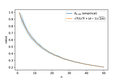
Refer to caption
Figure 6: Validity of Proposition 2 in the small n๐‘›n regime for Gaussian data (mean and 94% confidence interval of 50 independent samples for each value of n๐‘›n.
Proposition 4 (Proposition 2 restated).

Let ๐—โˆˆโ„nร—d๐—superscriptโ„๐‘›๐‘‘{\bf X}\in\mathbb{R}^{n\times d} and assume each ๐ฑi,ksubscript๐ฑ๐‘–๐‘˜{\bf x}_{i,k} is generated i.i.d. with zero-mean finite second moment ฯƒ2>0superscript๐œŽ20\sigma^{2}>0. Then the share of diagonal mass of the expected matrix ๐”ผโ€‹[|๐‡ols|]๐”ผdelimited-[]subscript๐‡ols\mathbb{E}\left[|{\bf H}_{\text{ols}}|\right] amounts to

ฮด๐”ผโ€‹[|๐‡ols|]โ€‹โ†’nโ†’โˆžโ€‹nn+(dโˆ’1)โ€‹2ฯ€subscript๐›ฟ๐”ผdelimited-[]subscript๐‡olsโ†’๐‘›โ†’๐‘›๐‘›๐‘‘12๐œ‹\delta_{\mathbb{E}\left[|{\bf H}_{\text{ols}}|\right]}\overset{n\rightarrow\infty}{\rightarrow}\frac{\sqrt{n}}{\sqrt{n}+(d-1)\sqrt{\frac{2}{\pi}}} (45)
Proof.
ฮด๐”ผโ€‹[|๐‡ols|]subscript๐›ฟ๐”ผdelimited-[]subscript๐‡ols\displaystyle\delta_{\mathbb{E}\left[|{\bf H}_{\text{ols}}|\right]} =โˆ‘k=1d๐”ผโ€‹[|(๐‡ols)k,k|]โˆ‘k=1dโˆ‘l=1d๐”ผโ€‹[|(๐‡ols)k,l|]=โˆ‘k=1d๐”ผโ€‹[|โˆ‘i=1n๐ฑi,k2|]โˆ‘k=1dโˆ‘l=1d๐”ผโ€‹[|โˆ‘i=1n๐ฑi,kโ€‹๐ฑi,l|]absentsuperscriptsubscript๐‘˜1๐‘‘๐”ผdelimited-[]subscriptsubscript๐‡ols๐‘˜๐‘˜superscriptsubscript๐‘˜1๐‘‘superscriptsubscript๐‘™1๐‘‘๐”ผdelimited-[]subscriptsubscript๐‡ols๐‘˜๐‘™superscriptsubscript๐‘˜1๐‘‘๐”ผdelimited-[]superscriptsubscript๐‘–1๐‘›superscriptsubscript๐ฑ๐‘–๐‘˜2superscriptsubscript๐‘˜1๐‘‘superscriptsubscript๐‘™1๐‘‘๐”ผdelimited-[]superscriptsubscript๐‘–1๐‘›subscript๐ฑ๐‘–๐‘˜subscript๐ฑ๐‘–๐‘™\displaystyle=\frac{\sum_{k=1}^{d}\mathbb{E}\left[|({\bf H}_{\text{ols}})_{k,k}|\right]}{\sum_{k=1}^{d}\sum_{l=1}^{d}\mathbb{E}\left[|({\bf H}_{\text{ols}})_{k,l}|\right]}=\frac{\sum_{k=1}^{d}\mathbb{E}\left[|\sum_{i=1}^{n}{\bf x}_{i,k}^{2}|\right]}{\sum_{k=1}^{d}\sum_{l=1}^{d}\mathbb{E}\left[|\sum_{i=1}^{n}{\bf x}_{i,k}{\bf x}_{i,l}|\right]} (46)
=dโ€‹โˆ‘i=1n๐”ผโ€‹[๐ฑi,12]dโ€‹โˆ‘i=1n๐”ผโ€‹[๐ฑi,12]+dโ€‹(dโˆ’1)โ€‹๐”ผโ€‹[|โˆ‘i=1n๐ฑi,1โ€‹๐ฑi,2|]absent๐‘‘superscriptsubscript๐‘–1๐‘›๐”ผdelimited-[]superscriptsubscript๐ฑ๐‘–12๐‘‘superscriptsubscript๐‘–1๐‘›๐”ผdelimited-[]superscriptsubscript๐ฑ๐‘–12๐‘‘๐‘‘1๐”ผdelimited-[]superscriptsubscript๐‘–1๐‘›subscript๐ฑ๐‘–1subscript๐ฑ๐‘–2\displaystyle=\frac{d\sum_{i=1}^{n}\mathbb{E}\left[{\bf x}_{i,1}^{2}\right]}{d\sum_{i=1}^{n}\mathbb{E}\left[{\bf x}_{i,1}^{2}\right]+d(d-1)\mathbb{E}\left[\left|\sum_{i=1}^{n}{\bf x}_{i,1}{\bf x}_{i,2}\right|\right]}

Where we used the fact that all ๐ฑi,ksubscript๐ฑ๐‘–๐‘˜{\bf x}_{i,k} are i.i.d. variables. Per assumption, we have ๐”ผโ€‹[๐ฑi,12]=ฯƒ2,โˆ€i๐”ผdelimited-[]superscriptsubscript๐ฑ๐‘–12superscript๐œŽ2for-all๐‘–\mathbb{E}\left[{\bf x}_{i,1}^{2}\right]=\sigma^{2},\forall i. Furthermore, the products ๐ฑi,1โ€‹๐ฑi,2subscript๐ฑ๐‘–1subscript๐ฑ๐‘–2{\bf x}_{i,1}{\bf x}_{i,2} are i.i.d with expectation 0 and variance ฯƒ4superscript๐œŽ4\sigma^{4}. By the central limit theorem

ZN=1nโ€‹โˆ‘i=1n๐ฑi,1โ€‹๐ฑi,2โ†’Zsubscript๐‘๐‘1๐‘›superscriptsubscript๐‘–1๐‘›subscript๐ฑ๐‘–1subscript๐ฑ๐‘–2โ†’๐‘Z_{N}=\frac{1}{\sqrt{n}}\sum_{i=1}^{n}{\bf x}_{i,1}{\bf x}_{i,2}\rightarrow Z

in law, with Zโˆผ๐’ฉโ€‹(0,ฯƒ4)similar-to๐‘๐’ฉ0superscript๐œŽ4Z\sim{\cal N}(0,\sigma^{4}), since ๐”ผโ€‹[Zn2]=1nโ€‹๐”ผโ€‹[(โˆ‘i=1n๐ฑi,1โ€‹๐ฑi,2)2]=1nโ€‹โˆ‘i=1n๐”ผโ€‹[๐ฑi,12]โ€‹๐”ผโ€‹[๐ฑi,22]=ฯƒ4๐”ผdelimited-[]superscriptsubscript๐‘๐‘›21๐‘›๐”ผdelimited-[]superscriptsuperscriptsubscript๐‘–1๐‘›subscript๐ฑ๐‘–1subscript๐ฑ๐‘–221๐‘›superscriptsubscript๐‘–1๐‘›๐”ผdelimited-[]superscriptsubscript๐ฑ๐‘–12๐”ผdelimited-[]superscriptsubscript๐ฑ๐‘–22superscript๐œŽ4\mathbb{E}\left[Z_{n}^{2}\right]=\frac{1}{n}\mathbb{E}\left[\left(\sum_{i=1}^{n}{\bf x}_{i,1}{\bf x}_{i,2}\right)^{2}\right]=\frac{1}{n}\sum_{i=1}^{n}\mathbb{E}[{\bf x}_{i,1}^{2}]\mathbb{E}[{\bf x}_{i,2}^{2}]=\sigma^{4} due to the independence assumption. Then Eโ€‹(|ZN|โ€‹โ€„1|ZN|โ‰ฅR)โ‰คEโ€‹(|ZN|2/R)โ‰คฯƒ4/R๐ธsubscript๐‘๐‘subscript1subscript๐‘๐‘๐‘…๐ธsuperscriptsubscript๐‘๐‘2๐‘…superscript๐œŽ4๐‘…E\left(\;|Z_{N}|\;1_{|Z_{N}|\geq R}\right)\ \leq\ E(|Z_{N}|^{2}/R)\leq\sigma^{4}/R. This implies that

Eโ€‹(|ZN|)โ†’Eโ€‹(|Z|)=2ฯ€โ€‹ฯƒ2โ†’๐ธsubscript๐‘๐‘๐ธ๐‘2๐œ‹superscript๐œŽ2E\left(\left|Z_{N}\right|\right)\rightarrow E(|Z|)=\sqrt{\frac{2}{\pi}}\sigma^{2}

As a result, we have that in the limit of large n๐‘›n

ฮด๐”ผโ€‹[|๐‡ols|]โ€‹โ†’nโ†’โˆžโ€‹dโ€‹nโ€‹ฯƒ2dโ€‹nโ€‹ฯƒ2+dโ€‹(dโˆ’1)โ€‹nโ€‹2ฯ€โ€‹ฯƒ2=11+(dโˆ’1)โ€‹2ฯ€n=nn+(dโˆ’1)โ€‹2ฯ€subscript๐›ฟ๐”ผdelimited-[]subscript๐‡olsโ†’๐‘›โ†’๐‘‘๐‘›superscript๐œŽ2๐‘‘๐‘›superscript๐œŽ2๐‘‘๐‘‘1๐‘›2๐œ‹superscript๐œŽ211๐‘‘12๐œ‹๐‘›๐‘›๐‘›๐‘‘12๐œ‹\delta_{\mathbb{E}\left[|{\bf H}_{\text{ols}}|\right]}\overset{n\rightarrow\infty}{\rightarrow}\frac{dn\sigma^{2}}{dn\sigma^{2}+d(d-1)\sqrt{n}\sqrt{\frac{2}{\pi}}\sigma^{2}}=\frac{1}{1+\frac{(d-1)\sqrt{\frac{2}{\pi}}}{\sqrt{n}}}=\frac{\sqrt{n}}{\sqrt{n}+(d-1)\sqrt{\frac{2}{\pi}}} (47)

โˆŽ

Appendix B: Background on second-order optimization

Appendix E Newtonโ€™s Method

The canonical second-order method is Newtonโ€™s methods. This algorithm uses the inverse Hessian as a scaling matrix and thus has updates of the form

๐ฐt+1=๐ฐtโˆ’โˆ‡2โ„’โ€‹(๐ฐt)โˆ’1โ€‹โˆ‡โ„’โ€‹(๐ฐt),subscript๐ฐ๐‘ก1subscript๐ฐ๐‘กsuperscriptโˆ‡2โ„’superscriptsubscript๐ฐ๐‘ก1โˆ‡โ„’subscript๐ฐ๐‘ก{\bf w}_{t+1}={\bf w}_{t}-\nabla^{2}\mathcal{L}({\bf w}_{t})^{-1}\nabla\mathcal{L}({\bf w}_{t}), (48)

which is equivalent to optimizing the local quadratic model

mNโ€‹(๐ฐt):=โ„’โ€‹(๐ฐt)+โˆ‡โ„’โ€‹(๐ฐt)โŠบโ€‹๐ฌ+12โ€‹๐ฌโŠบโ€‹โˆ‡2โ„’โ€‹(๐ฐt)โ€‹๐ฌassignsubscript๐‘š๐‘subscript๐ฐ๐‘กโ„’subscript๐ฐ๐‘กโˆ‡โ„’superscriptsubscript๐ฐ๐‘กโŠบ๐ฌ12superscript๐ฌโŠบsuperscriptโˆ‡2โ„’subscript๐ฐ๐‘ก๐ฌm_{N}({\bf w}_{t}):=\mathcal{L}({\bf w}_{t})+\nabla\mathcal{L}({\bf w}_{t})^{\intercal}{\bf s}+\frac{1}{2}{\bf s}^{\intercal}\nabla^{2}\mathcal{L}({\bf w}_{t}){\bf s} (49)

to first-order stationarity. Using curvature information to rescale the steepest descent direction gives Newtonโ€™s method the useful property of being linearly scale invariant. This gives rise to a problem independent local convergence rate that is super-linear and even quadratic in the case of Lipschitz continuous Hessians (see [51] Theorem 3.5), whereas gradient descent at best achieves linear local convergence [49].

However, there are certain drawbacks associated with applying classical Newtonโ€™s method. First of all, the Hessian matrix may be singular and thus not invertible. Secondly, even if it is invertible the local quadratic model (Eq.ย 49) that is minimized in each NM iteration may simply be an inadequate approximation of the true objective. As a result, the Newton step is not necessarily a descent step. It may hence approximate arbitrary critical points (including local maxima) or even diverge. Finally, the cost of forming and inverting the Hessian sum up to Oโ€‹(nโ€‹d2+d3)๐‘‚๐‘›superscript๐‘‘2superscript๐‘‘3O(nd^{2}+d^{3}) and are thus prohibitively high for applications in large dimensional problems.

Appendix F Trust Region Methods

F.1 Outer iterations

Trust region methods are among the most principled approaches to overcome the above mentioned issues. These methods also construct a quadratic model mtsubscript๐‘š๐‘กm_{t} but constrain the subproblem in such a way that the stepsize is restricted to stay within a certain radius ฮ”tsubscriptฮ”๐‘ก\Delta_{t} within which the model is trusted to be sufficiently adequate

minsโˆˆโ„dโกmtโ€‹(๐ฌ)=โ„’โ€‹(๐ฐt)+โˆ‡โ„’โ€‹(๐ฐt)โŠบโ€‹๐ฌ+12โ€‹๐ฌโŠบโ€‹โˆ‡2โ„’โ€‹(๐ฐt)โ€‹๐ฌ,s.t.โ€–๐ฌโ€–โ‰คฮ”t.formulae-sequencesubscript๐‘ superscriptโ„๐‘‘subscript๐‘š๐‘ก๐ฌโ„’subscript๐ฐ๐‘กโˆ‡โ„’superscriptsubscript๐ฐ๐‘กโŠบ๐ฌ12superscript๐ฌโŠบsuperscriptโˆ‡2โ„’subscript๐ฐ๐‘ก๐ฌ๐‘ ๐‘กnorm๐ฌsubscriptฮ”๐‘ก\min_{s\in\mathbb{R}^{d}}\>m_{t}({\bf s})=\mathcal{L}({\bf w}_{t})+\nabla\mathcal{L}({\bf w}_{t})^{\intercal}{\bf s}+\frac{1}{2}{\bf s}^{\intercal}\nabla^{2}\mathcal{L}({\bf w}_{t}){\bf s},\>\>\>s.t.\>\|{\bf s}\|\leq\Delta_{t}. (50)

Hence, contrary to line-search methods this approach finds the step ๐ฌtsubscript๐ฌ๐‘ก{\bf s}_{t} and its length โ€–๐ฌtโ€–normsubscript๐ฌ๐‘ก{}\left\|{\bf s}_{t}\right\| simultaneously by optimizing (50). Subsequently the actual decrease โ„’โ€‹(๐ฐt)โˆ’โ„’โ€‹(๐ฐt+๐ฌt)โ„’subscript๐ฐ๐‘กโ„’subscript๐ฐ๐‘กsubscript๐ฌ๐‘ก\mathcal{L}({\bf w}_{t})-\mathcal{L}({\bf w}_{t}+{\bf s}_{t}) is compared to the predicted decrease mtโ€‹(0)โˆ’mtโ€‹(๐ฌt)subscript๐‘š๐‘ก0subscript๐‘š๐‘กsubscript๐ฌ๐‘กm_{t}(0)-m_{t}({\bf s}_{t}) and the step is only accepted if the ratio ฯ:=โ„’โ€‹(๐ฐt)โˆ’โ„’โ€‹(๐ฐt+๐ฌt)/(mtโ€‹(0)โˆ’mtโ€‹(๐ฌt))assign๐œŒโ„’subscript๐ฐ๐‘กโ„’subscript๐ฐ๐‘กsubscript๐ฌ๐‘กsubscript๐‘š๐‘ก0subscript๐‘š๐‘กsubscript๐ฌ๐‘ก\rho:=\mathcal{L}({\bf w}_{t})-\mathcal{L}({\bf w}_{t}+{\bf s}_{t})/(m_{t}(0)-m_{t}({\bf s}_{t})) exceeds some predefined success threshold ฮท1>0subscript๐œ‚10\eta_{1}>0. Furthermore, the trust region radius is decreased whenever ฯ๐œŒ\rho falls below ฮท1subscript๐œ‚1\eta_{1} and it is increased whenever ฯ๐œŒ\rho exceeds the โ€very successfulโ€ threshold ฮท2โ€‹0subscript๐œ‚20\eta_{2}0. Thereby, the algorithm adaptively measures the accuracy of the second-order Taylor model โ€“ which may change drastically over the parameter space depending on the behaviour of the higher-order derivatives999Note that the second-order Taylor models assume constant curvature. โ€“ and adapts the effective length along which the model is trusted accordingly. See [19] for more details.

As a consequence, the plain Newton step ๐ฌN,t=โˆ’(โˆ‡2โ„’t)โˆ’1โ€‹โˆ‡โ„’tsubscript๐ฌ๐‘๐‘กsuperscriptsuperscriptโˆ‡2subscriptโ„’๐‘ก1โˆ‡subscriptโ„’๐‘ก{\bf s}_{N,t}=-\left(\nabla^{2}\mathcal{L}_{t}\right)^{-1}\nabla\mathcal{L}_{t} is only taken if it lies within the trust region radius and yields a certain amount of decrease in the objective value. Since many functions look somehow quadratic close to a minimizer the radius can be shown to grow asymptotically under mild assumptions such that eventually full Newton steps are taken in every iteration which retains the local quadratic convergence rate [19].

Figure 7: Level sets of the non-convex, coercive objective function fโ€‹(๐ฐ)=0.5โ€‹๐ฐ02+0.25โ€‹๐ฐ14โˆ’0.5โ€‹๐ฐ12๐‘“๐ฐ0.5superscriptsubscript๐ฐ020.25superscriptsubscript๐ฐ140.5superscriptsubscript๐ฐ12f({\bf w})=0.5{\bf w}_{0}^{2}+0.25{\bf w}_{1}^{4}-0.5{\bf w}_{1}^{2}. Newtonโ€™s Method makes a local quadratic model (blue dashed lines) and steps to its critical point. It may be thus be ascending (left) or attracted by a saddle point (right). TR methods relieve this issue by stepping to the minimizer of that model within a certain region (green dashed line).

F.2 Subproblem solver

Interestingly, there is no need to optimize Eq.ย (50) to global optimality to retain the remarkable global convergence properties of TR algorithms. Instead, it suffices to do better than the Cauchy- and Eigenpoint101010which are the model minimizers along the gradient and the eigendirection associated with its smallest eigenvalue, respectively. simultaneously. One popular approach is to minimize mtโ€‹(๐ฌ)subscript๐‘š๐‘ก๐ฌm_{t}({\bf s}) in nested Krylov subspaces. These subspaces naturally include the gradient direction as well as increasingly accurate estimates of the leading eigendirection

spanโ€‹{๐ t,๐tโ€‹๐ t,๐t2โ€‹๐ t,โ€ฆ,๐tjโ€‹๐ t}spansubscript๐ ๐‘กsubscript๐๐‘กsubscript๐ ๐‘กsuperscriptsubscript๐๐‘ก2subscript๐ ๐‘กโ€ฆsuperscriptsubscript๐๐‘ก๐‘—subscript๐ ๐‘ก\text{span}\{{\bf g}_{t},{\bf B}_{t}{\bf g}_{t},{\bf B}_{t}^{2}{\bf g}_{t},\ldots,{\bf B}_{t}^{j}{\bf g}_{t}\} (51)

until (for example) the stopping criterion

โ€–โˆ‡mtโ€‹(๐ฌj)โ€–โ‰คโ€–โˆ‡โ„’โ€‹(๐ฐt)โ€–โ€‹minโก{ฮบK,โ€–โˆ‡โ„’โ€‹(๐ฐt)โ€–ฮธ},ฮบK<1,ฮธโ‰ฅ0formulae-sequencenormโˆ‡subscript๐‘š๐‘กsubscript๐ฌ๐‘—normโˆ‡โ„’subscript๐ฐ๐‘กsubscript๐œ…๐พsuperscriptnormโˆ‡โ„’subscript๐ฐ๐‘ก๐œƒformulae-sequencesubscript๐œ…๐พ1๐œƒ0\|\nabla m_{t}({\bf s}_{j})\|\leq\|\nabla\mathcal{L}({\bf w}_{t})\|\min\{\kappa_{K},\|\nabla\mathcal{L}({\bf w}_{t})\|^{\theta}\},\quad\kappa_{K}<1,\theta\geq 0 (52)

is met, which requires increased accuracy as the underlying trust region algorithm approaches criticality. Conjugate gradients and Lanczos method are two iterative routines that implicitly build up a conjugate and orthogonal basis for such a Krylov space respectively and they converge linearly on quadratic objectives with a square-root dependency on the condition number of the Hessianย [19]. We here employ the preconditionied Steihaug-Toint CG method [60] in order to cope with possible boundary solutions of (50) but similar techniques exist for the Lanczos solver as well for which we also provide code. As preconditioning matrix for CG we use the same matrix as for the ellipsoidal constraint.

Appendix G Damped (Gauss-)Newton methods

An alternative approach to actively constraining the region within which the model is trusted is to instead penalize the step norm in each iteration in a Lagrangian manner. This is done by so-called damped Newton methods that add a ฮป>0๐œ†0\lambda>0 multiple of the identity matrix to the second-order term in the model, which leads to the update step

minsโˆˆโ„dโกmtโ€‹(๐ฌ)subscript๐‘ superscriptโ„๐‘‘subscript๐‘š๐‘ก๐ฌ\displaystyle\min_{s\in\mathbb{R}^{d}}\>m_{t}({\bf s}) =โ„’โ€‹(๐ฐt)+โˆ‡โ„’โ€‹(๐ฐt)โŠบโ€‹๐ฌ+12โ€‹๐ฌโŠบโ€‹(โˆ‡2โ„’โ€‹(๐ฐt)+ฮปโ€‹๐ˆ)โ€‹๐ฌabsentโ„’subscript๐ฐ๐‘กโˆ‡โ„’superscriptsubscript๐ฐ๐‘กโŠบ๐ฌ12superscript๐ฌโŠบsuperscriptโˆ‡2โ„’subscript๐ฐ๐‘ก๐œ†๐ˆ๐ฌ\displaystyle=\mathcal{L}({\bf w}_{t})+\nabla\mathcal{L}({\bf w}_{t})^{\intercal}{\bf s}+\frac{1}{2}{\bf s}^{\intercal}(\nabla^{2}\mathcal{L}({\bf w}_{t})+\lambda\mathbf{I}){\bf s} (53)
=โ„’โ€‹(๐ฐt)+โˆ‡โ„’โ€‹(๐ฐt)โŠบโ€‹๐ฌ+12โ€‹๐ฌโŠบโ€‹โˆ‡2โ„’โ€‹(๐ฐt)โ€‹๐ฌ+ฮปโ€‹โ€–๐ฌโ€–2.absentโ„’subscript๐ฐ๐‘กโˆ‡โ„’superscriptsubscript๐ฐ๐‘กโŠบ๐ฌ12superscript๐ฌโŠบsuperscriptโˆ‡2โ„’subscript๐ฐ๐‘ก๐ฌ๐œ†superscriptnorm๐ฌ2\displaystyle=\mathcal{L}({\bf w}_{t})+\nabla\mathcal{L}({\bf w}_{t})^{\intercal}{\bf s}+\frac{1}{2}{\bf s}^{\intercal}\nabla^{2}\mathcal{L}({\bf w}_{t}){\bf s}+\lambda\|{\bf s}\|^{2}.

This can also be solved hessian-free by conjugate gradients (or other Krylov subspace methods). The penalty parameter ฮป๐œ†\lambda is acting inversely to the trust region radius ฮ”ฮ”\Delta and it is often updated accordingly. Such algorithms are commonly known as Levenberg-Marquardt algorithms and they were originally tailored towards solving non-linear least squares problems [51] but they have been proposed for neural network training already early on [33].

Many algorithms in the existing literature replace the use of โˆ‡2โ„’โ€‹(๐ฐt)superscriptโˆ‡2โ„’subscript๐ฐ๐‘ก\nabla^{2}\mathcal{L}({\bf w}_{t}) in (53) with the Generalized Gauss Newton matrixย [44, 17] or an approximation of the latter [46]. This matrix constitutes the first part of the well-known Gauss-Newton decomposition

โˆ‡2โ„’โ€‹(โ‹…)=1nโ€‹โˆ‘i=1nโ„“โ€ฒโ€ฒโ€‹(fiโ€‹(โ‹…))โ€‹โˆ‡fiโ€‹(โ‹…)โ€‹โˆ‡fiโ€‹(โ‹…)โŠบโŸ:=๐€Gโ€‹Gโ€‹N+1nโ€‹โˆ‘i=1nโ„“โ€ฒโ€‹(fiโ€‹(โ‹…))โ€‹โˆ‡2fiโ€‹(โ‹…),superscriptโˆ‡2โ„’โ‹…subscriptโŸ1๐‘›superscriptsubscript๐‘–1๐‘›superscriptโ„“โ€ฒโ€ฒsubscript๐‘“๐‘–โ‹…โˆ‡subscript๐‘“๐‘–โ‹…โˆ‡subscript๐‘“๐‘–superscriptโ‹…โŠบassignabsentsubscript๐€๐บ๐บ๐‘1๐‘›superscriptsubscript๐‘–1๐‘›superscriptโ„“โ€ฒsubscript๐‘“๐‘–โ‹…superscriptโˆ‡2subscript๐‘“๐‘–โ‹…\nabla^{2}\mathcal{L}(\cdot)=\underbrace{\frac{1}{n}\sum_{i=1}^{n}\ell^{\prime\prime}(f_{i}(\cdot))\nabla f_{i}(\cdot)\nabla f_{i}(\cdot)^{\intercal}}_{:={\bf A}_{GGN}}+\frac{1}{n}\sum_{i=1}^{n}\ell^{\prime}(f_{i}(\cdot))\nabla^{2}f_{i}(\cdot), (54)

where lโ€ฒsuperscript๐‘™โ€ฒl^{\prime} and lโ€ฒโ€ฒsuperscript๐‘™โ€ฒโ€ฒl^{\prime\prime} are the first and second derivative of l:โ„oโ€‹uโ€‹tโ†’โ„+:๐‘™โ†’superscriptโ„๐‘œ๐‘ข๐‘กsuperscriptโ„l:\mathbb{R}^{out}\rightarrow\mathbb{R}^{+} assuming that oโ€‹uโ€‹t=1๐‘œ๐‘ข๐‘ก1out=1 (binary classification and regression task) for simplicity here.

It is interesting to note that the GGN matrix ๐€Gโ€‹Gโ€‹Nsubscript๐€๐บ๐บ๐‘{\bf A}_{GGN} of neural networks is equivalent to the Fisher matrix used in natural gradient descentย [5] in many cases like linear activation function and squared error as well as sigmoid and cross-entropy or softmax and negative log-likelihood for which the extended Gauss-Newton is defined [53]. As can be seen in (54) the matrix ๐€Gโ€‹Gโ€‹Nsubscript๐€๐บ๐บ๐‘{\bf A}_{GGN} is positive semidefinite (and low rank if n<d๐‘›๐‘‘n<d). As a result, there exist no second-order convergence guarantees for such methods on general non-convex problems. On the other end of the spectrum, the GGN also drops possibly positive terms from the Hessian (see 54). Hence it is not guaranteed to be an upper bound on the latter in the PSD sense. Essentially, GGN approximations assume that the network is piece-wise linear and thus the GGN and Hessian matrices only coincide in the case of linear and ReLU activations or non-curved loss functions. For any other activation the GGN matrix may approximate the Hessian only asymptotically and if the โ„“โ€ฒโ€‹(fiโ€‹(โ‹…))superscriptโ„“โ€ฒsubscript๐‘“๐‘–โ‹…\ell^{\prime}(f_{i}(\cdot)) terms in 54 go to zero for all iโˆˆ{1,โ€ฆ,n}๐‘–1โ€ฆ๐‘›i\in\{1,\ldots,n\}. In non-linear least squares such problems are called zero-residual problems and GN methods can be shown to have quadratic local convergence there. In any other case the convergence rate does not exceed the linear local convergence bound of gradient descent. In practice however there are cases where deep neural nets do show negative curvature in the neighborhood of a minimizerย [10].Finally, [23] propose the use of the absolute Hessian instead of the GGN matrix in a framework similar to 53. This method has been termed saddle-free Newton even though its manifold of attraction to a given saddle is non-empty111111It is the same as that for GD, which renders the method unable to escape e.g. when initialized right on a saddle point. To be fair, the manifold of attraction for GD constitutes a measure zero setย [39]..

Figure 8: Both, the GGN method and saddle-free Newton method make a positive definite quadratic model around the current iterate and thereby overcome the abstractedness of pure Newton towards the saddle (compare Figure 7). However, (i) none of these methods can escape the saddle once they are in the gradient manifold of attraction and (ii) as reported in [48] the GN matrix can be significantly less well conditioned than the absolute Hessian (here ฮบGโ€‹N=49โ€ฒโ€‹487โ€ฒโ€‹554subscript๐œ…๐บ๐‘superscript49โ€ฒsuperscript487โ€ฒ554\kappa_{GN}=49^{\prime}487^{\prime}554 and ฮบ|H|=1.03subscript๐œ…๐ป1.03\kappa_{|H|}=1.03 so we had to add a damping factor of ฮป=0.1๐œ†0.1\lambda=0.1 to make the GN step fit the plot.

G.1 Comparison to trust region

Contrary to TR methods, the Levenberg-Marquardt methods never take plain Newton steps since the regularization is always on (ฮป>0๐œ†0\lambda>0). Furthermore, if a positive-definite Hessian approximation like the Generalized Gauss Newton matrix is used, this algorithm is not capable of exploiting negative curvature and there are cases in neural network training where the Hessian is much better conditioned than the Gauss-Newton matrix [48] (also see Figure 8). While some scholars believe that positive-definiteness is a desirable feature [44, 17], we want to point out that following negative curvature directions is necessarily needed to escape saddle points and it can also be meaningful to follow directions of negative eigenvalue ฮป๐œ†\lambda outside a saddle since they guarantee ๐’ชโ€‹(|ฮป|3)๐’ชsuperscript๐œ†3\mathcal{O}(|\lambda|^{3}) progress, whereas a gradient descent step yields at least โ€–โˆ‡fโ€‹(๐ฐ)โ€–2superscriptnormโˆ‡๐‘“๐ฐ2\|\nabla f({\bf w})\|^{2} progress (both under certain stepsize conditions) and one cannot conclude a-priori which one is better in general [20, 2]. Despite these theoretical considerations, many methods based on GGN matrices have been applied to neural network training (see [45] and references therein) and particularly the hessian-free implementations of [44, 17] can be implemented very cheaply [58].

Appendix H Using Hessian information in Neural Networks

While many theoretical arguments suggest the superiority of regularized Newton methods over gradient based algorithms, several practical considerations cast doubt on this theoretical superiority when it comes to neural network training. Answers to the following questions are particularly unclear: Are saddles even an issue in deep learning? Is superlinear local convergence a desirable feature in machine learning applications (test error)? Are second-order methods more โ€vulnerableโ€ to sub-sampling noise? Do worst-case iteration complexities even matter in real-world settings? As a result, the value of Hessian information in neural network training is somewhat unclear a-priori and so far a conclusive empirical study is still missing.

Our empirical findings indicate that the net value of Hessian information for neural network training is indeed somewhat limited for mainly three reasons: 1) second-order methods rarely yield better limit points, which suggests that saddles and spurious local minima are not a major obstacle; 2) gradient methods can indeed run on smaller batch sizes which is beneficial in terms of epoch and when memory is limited; 3) The per-iteration time complexity is noticeably lower for first-order methods. In summary, these observations suggest that advances in hardware and distributed second-order algorithms (e.g., ย [52, 28]) will be needed before Newton-type methods can replace (stochastic) gradient methods in deep learning.

Appendix C: Experiment details

Appendix I Ellipsoidal Trust Region vs. First-order Optimizers

To put the previous results into context, we also benchmark several state-of-the-art gradient methods. We fix their sample size to 32 (as advocated e.g. in [47]) but grid search the stepsize, since it is the ratio of these two quantities that effectively determines the level of stochasticityย [35]. The TR methods use a batch size of 128 for the ResNet architecture and 512 otherwise121212We observed weaker performance when running with smaller batches, presumably because second-order methods are likely to โ€overfitโ€ noise in small batches in any given iteration as they extract more information of each batch per step by computing curvature.. For a fair comparison, we thus report results in terms of number of backpropagations, epochs and time . The findings are mixed: For small nets such as the MLPs the TR method with RMSProp ellipsoids is superior in all metrics, even when benchmarked in terms of time. However, while Fig. 9 indicates that ellipsoidal TR methods are slightly superior in terms of backpropagations even for bigger nets (ResNets and Autoencoders), a close look at the Figures 10 and 11 (App. C) reveals that they at best manage to keep pace with first-order methods in terms of epochs and are inferior in time. Furthermore, only the autoencoders give rise to a saddle point, which adaptive gradient methods escape faster than vanilla SGD, just like it was the case for second-order methods (see Fig. 3).

MLP ResNet Autoencoder

Fashion-MNIST

Refer to caption Refer to caption Refer to caption

CIFAR-10

Refer to caption Refer to caption Refer to caption
Figure 9: Log loss over backpropagations. Same setting as Figureย 3. See Figureย 10 for epoch results.
ResNet18 Fully-Connected Autoencoder

CIFAR-10

Refer to caption Refer to caption Refer to caption

Fashion-MNIST

Refer to caption Refer to caption Refer to caption
Figure 10: Experiment comparing TR and gradient methods in terms of epochs. Average log loss as well as 95%percent9595\% confidence interval shown.
ResNet18 Fully-Connected Autoencoder

CIFAR-10

Refer to caption Refer to caption Refer to caption

Fashion-MNIST

Refer to caption Refer to caption Refer to caption
Figure 11: Experiment comparing TR and gradient methods in terms of wall-clock time. Average log loss as well as 95%percent9595\% confidence interval shown. The advantage of extremely low-iteration costs of first-order methods is particularly notable in the ResNet18 architecture due to the large network size.

Appendix J Default parameters, architectures and datasets

Parameters

Table 1 reports the default parameters we consider. Only for the larger ResNet18 on CIFAR-10, we adapted the batch size to 128128128 due to memory constraints.

|๐’ฎ0|subscript๐’ฎ0|\mathcal{S}_{0}| ฮ”0subscriptฮ”0\Delta_{0} ฮ”maxsubscriptฮ”max\Delta_{\text{max}} ฮท1subscript๐œ‚1\eta_{1} ฮท2subscript๐œ‚2\eta_{2} ฮณ1subscript๐›พ1\gamma_{1} ฮณ2subscript๐›พ2\gamma_{2} ฮบKsubscript๐œ…๐พ\kappa_{K} (krylov tol.)
TRuniuni{}_{\text{uni}} 512 10โˆ’4superscript10410^{-4} 10 10โˆ’4superscript10410^{-4} 0.95 1.1 1.5 0.1
TRadaada{}_{\text{ada}} 512 10โˆ’4superscript10410^{-4} 10 10โˆ’4superscript10410^{-4} 0.95 1.1 1.5 0.1
TRrmsrms{}_{\text{rms}} 512 10โˆ’4superscript10410^{-4} 10 10โˆ’4superscript10410^{-4} 0.95 1.1 1.75 0.1
Table 1: Default parameters
Datasets

We use two real-world datasets for image classification, namely CIFAR-10 and Fashion-MNIST131313Both datasets were accessed from https://www.tensorflow.org/api_docs/python/tf/keras/datasets. While Fashion-MNIST consists of greyscale 28ร—28282828\times 28 images, CIFAR-10 are colored images of size 32ร—32323232\times 32. Both datasets have a fixed training-test split consisting of 60,000 and 10,000 images, respectively.

Network architectures

The MLP architectures are simple. For MNIST and Fashion-MNIST we use a 784โˆ’128โˆ’1078412810784-128-10 network with tanh activations and a cross entropy loss. The networks has 101โ€ฒโ€‹770superscript101โ€ฒ770101^{\prime}770 parameters. For the CIFAR-10 MLP we use a 3072โˆ’128โˆ’128โˆ’103072128128103072-128-128-10 architecture also with tanh activations and cross entropy loss. This network has 410โ€ฒโ€‹880superscript410โ€ฒ880410^{\prime}880 parameters.

The Fashion-MNIST autoencoder has the same architecture as the one used in [34, 66, 44, 46]. The encoder structure is 784โˆ’1000โˆ’500โˆ’250โˆ’30784100050025030784-1000-500-250-30 and the decoder is mirrored. Sigmoid activations are used in all but the central layer. The reconstructed images are fed pixelwise into a binary cross entropy loss. The network has a total of 2โ€ฒโ€‹833โ€ฒโ€‹000superscript2โ€ฒsuperscript833โ€ฒ0002^{\prime}833^{\prime}000 parameters. The CIFAR-10 autoencoder is taken from the implementation of https://github.com/jellycsc/PyTorch-CIFAR-10-autoencoder.

For the ResNet18, we used the implementation from torchvision for CIFAR-10 as well as a modification of it for Fashion-MNIST that adapts the first convolution to account for the single input channel.

In all of our experiments each method was run on one Tesla P100 GPU using the PyTorch [54] library.

Appendix K Reconstructed Images from Autoencoders

Original SGD Adagrad Rmsprop TR Uniform TR Adagrad TR RMSprop
Refer to caption Refer to caption Refer to caption Refer to caption Refer to caption Refer to caption Refer to caption Refer to caption Refer to caption Refer to caption Refer to caption Refer to caption Refer to caption Refer to caption Refer to caption Refer to caption Refer to caption Refer to caption Refer to caption Refer to caption Refer to caption
Figure 12: Original and reconstructed MNIST digits (left), Fashion-MNIST items (middle), and CIFAR-10 classes (right) for different optimization methods after convergence.