Learning Robust Options
by Conditional Value at Risk Optimization

Takuya Hiraoka NEC Corporation National Institute of Advanced Industrial Science and Technology RIKEN Center for Advanced Intelligence Project Takahisa Imagawa National Institute of Advanced Industrial Science and Technology Tatsuya Mori NEC Corporation National Institute of Advanced Industrial Science and Technology RIKEN Center for Advanced Intelligence Project Takashi Onishi NEC Corporation National Institute of Advanced Industrial Science and Technology Yoshimasa Tsuruoka National Institute of Advanced Industrial Science and Technology The University of Tokyo
Abstract

Options are generally learned by using an inaccurate environment model (or simulator), which contains uncertain model parameters. While there are several methods to learn options that are robust against the uncertainty of model parameters, these methods only consider either the worst case or the average (ordinary) case for learning options. This limited consideration of the cases often produces options that do not work well in the unconsidered case. In this paper, we propose a conditional value at risk (CVaR)-based method to learn options that work well in both the average and worst cases. We extend the CVaR-based policy gradient method proposed by Chow and Ghavamzadeh (2014) to deal with robust Markov decision processes and then apply the extended method to learning robust options. We conduct experiments to evaluate our method in multi-joint robot control tasks (HopperIceBlock, Half-Cheetah, and Walker2D). Experimental results show that our method produces options that 1) give better worst-case performance than the options learned only to minimize the average-case loss, and 2) give better average-case performance than the options learned only to minimize the worst-case loss.

1 Introduction

In the reinforcement learning context, an Option means a temporally extended sequence of actions [30], and is regarded as useful for many purposes, such as speeding up learning, transferring skills across domains, and solving long-term planning problems. Because of its usefulness, the methods for discovering (learning) options have been actively studied (e.g., [1, 17, 18, 20, 28, 29]).

Learning options successfully in practical domains requires a large amount of training data, but collecting data from a real-world environment is often prohibitively expensive [15]. In such cases, environment models (i.e., simulators) are used for learning options instead, but such models usually contain uncertain parameters (i.e., a reality gap) since they are constructed based on insufficient knowledge of a real environment. Options learned with an inaccurate model can lead to a significant degradation of the performance of the agent when deployed in the real environment [19]. This problem is a severe obstacle to applying the options framework to practical tasks in the real world, and has driven the need for methods that can learn robust options against inaccuracy of models.

Some previous work has addressed the problem of learning options that are robust against inaccuracy of models. Mankowitz et al. [19] proposed a method to learn options that minimize the expected loss (or maximize an expected return) on the environment model with the worst-case model parameter values, which are selected so that the expected loss is maximized. Frans et al. [10] proposed a method to learn options that minimize the expected loss on the environment model with the average-case model parameter values.

However, these methods only consider either the worst-case model parameter values or the average-case model parameter values when learning options, and this causes learned options to work poorly in an environment with the unconsidered model parameter values. Mankowitz’s [19] method produces options that are overly conservative in the environment with an average-case model parameter value [9]. In contrast, Frans’s method [10] produces options that can cause a catastrophic failure in an environment with the worst-case model parameter value.

Furthermore, Mankowitz’s [19] method does not use a distribution of the model parameters for learning options. Generally, the distribution can be built on the basis of prior knowledge. If the distribution can be used, as in Derman et al. [9] and Rajeswaran et al. [24], one can use it to adjust the importance of the model parameter values in learning options. However, Mankowitz’s method does not consider the distribution and always produces the policy to minimize the loss in the worst case model parameter value. Therefore, even if the worst case is extremely unlikely to happen, the learned policy is adapted to the case and results in being overly conservative.

To mitigate the aforementioned problems, we propose a conditional value at risk (CVaR)-based method to learn robust options optimized for the expected loss in both the average and worst cases. In our method, an option is learned so that it 1) makes the expected loss lower than a given threshold in the worst case and also 2) decreases the expected loss in the average case as much as possible. Since our method considers both the worst and average cases when learning options, it can mitigate the aforementioned problems with the previous methods for option learning. In addition, unlike Mankowitz’s [19] method, our method evaluates the expected loss in the worst case on the basis of CVaR (see Section 3). This enables us to reflect the model parameter distribution in learning options, and thus prevents the learned options from overfitting an environment with an extremely rare worst-case parameter value.

Our main contributions are as follows: (1) We introduce CVaR optimization to learning robust options and illustrate its effectiveness (see Section 3, Section 4, and Appendices). Although some previous works have proposed CVaR-based reinforcement learning methods (e.g., [6, 24, 32]), their methods have been applied to learning robust “flat” policies, and option learning has not been discussed. (2) We extend Chow and Ghavamzadeh’s CVaR-based policy gradient method [6] so that it can deal with robust Markov decision processes (robust MDPs) and option learning. Their method is for ordinary MDPs and does not take the uncertainty of model parameters into account. We extend their method to robust MDPs to deal with the uncertain model parameters (see Section 3). Further, we apply the extended method to learn robust options. For this application, we derive the option policy gradient theorem [1] to minimise soft robust loss [9] (see Appendices). (3) We evaluate our robust option learning methods in several nontrivial continuous control tasks (see Section 4 and Appendices). Robust option learning methods have not been thoroughly evaluated on such tasks. Mankowitz et al. [19] evaluated their methods only on simple control tasks (Acrobot and CartPole with discrete action spaces). Our research is a first attempt to evaluate robust option learning methods on more complex tasks (multi-joint robot control tasks) where state–action spaces are high dimensional and continuous.

This paper is organized as follows. First we define our problem and introduce preliminaries (Section 2), and then propose our method by extending Chow and Ghavamzadeh’s method (Section 3). We evaluate our method on multi-joint robot control tasks (Section 4). We also discuss related work (Section 5). Finally, we conclude our research.

2 Problem Description

We consider a robust MDP [34], which is tuple S,A,,γ,P,Tp,0𝑆𝐴𝛾𝑃subscript𝑇𝑝subscript0\langle S,A,\mathbb{C},\gamma,P,T_{p},\mathbb{P}_{0}\rangle where S𝑆S, A𝐴A, \mathbb{C}, γ𝛾\gamma, and P𝑃P are states, actions, a cost function, a discount factor, and an ambiguity set, respectively; Tpsubscript𝑇𝑝T_{p} and 0subscript0\mathbb{P}_{0} are a state transition function parameterized by pP𝑝𝑃p\in P, and an initial state distribution, respectively. The transition probability is used in the form of st+1Tp(st,at)similar-tosubscript𝑠𝑡1subscript𝑇𝑝subscript𝑠𝑡subscript𝑎𝑡s_{t+1}\sim T_{p}(s_{t},a_{t}), where st+1subscript𝑠𝑡1s_{t+1} is a random variable. Similarly, the initial state distribution is used in the form of s00similar-tosubscript𝑠0subscript0s_{0}\sim\mathbb{P}_{0}. The cost function is used in the form of ct+1(st,at)similar-tosubscript𝑐𝑡1subscript𝑠𝑡subscript𝑎𝑡c_{t+1}\sim\mathbb{C}(s_{t},a_{t}), where ct+1subscript𝑐𝑡1c_{t+1} is a random variable. Here, the sum of the costs discounted by γ𝛾\gamma is called a loss 𝒞=t=0Tγtct𝒞superscriptsubscript𝑡0𝑇superscript𝛾𝑡subscript𝑐𝑡\mathcal{C}=\sum_{t=0}^{T}\gamma^{t}c_{t}.

As with the standard robust reinforcement learning settings [9, 10, 24], p𝑝p is generated by a model parameter distribution (p)𝑝\mathbb{P}(p) that captures our subjective belief about the parameter values of a real environment. By using the distribution, we define a soft robust loss [9]:

𝔼𝒞,p[𝒞]=p(p)𝔼𝒞[𝒞p],subscript𝔼𝒞𝑝delimited-[]𝒞subscript𝑝𝑝subscript𝔼𝒞delimited-[]conditional𝒞𝑝\displaystyle\mathbb{E}_{\mathcal{C},p}\left[\mathcal{C}\right]=\sum_{p}\mathbb{P}(p)\mathbb{E}_{\mathcal{C}}\left[\mathcal{C}\mid p\right], (1)

where 𝔼𝒞[𝒞|p]subscript𝔼𝒞delimited-[]conditional𝒞𝑝\mathbb{E}_{\mathcal{C}}\left[\left.\mathcal{C}~{}\right|~{}p\right] is the expected loss on a parameterized MDP S,A,,γ,Tp,0𝑆𝐴𝛾subscript𝑇𝑝subscript0\langle S,A,\mathbb{C},\gamma,T_{p},\mathbb{P}_{0}\rangle, in which the transition probability is parameterized by p𝑝p.

As with Derman et al. [9] and Xu and Mannor [35], we make the rectangularity assumption on P𝑃P and (p)𝑝\mathbb{P}(p). That is, P𝑃P is assumed to be structured as a Cartesian product sSPssubscripttensor-product𝑠𝑆subscript𝑃𝑠\bigotimes_{s\in S}P_{s}, and \mathbb{P} is also assumed to be a Cartesian product sSs(psPs)subscripttensor-product𝑠𝑆subscript𝑠subscript𝑝𝑠subscript𝑃𝑠\bigotimes_{s\in S}\mathbb{P}_{s}(p_{s}\in P_{s}). These assumptions enable us to define a model parameter distribution independently for each state.

We also assume that the learning agent interacts with an environment on the basis of its policy, which takes the form of the call-and-return option [29]. Option ωΩ𝜔Ω\omega\in\Omega is a temporally extended action and represented as a tuple Iω,πω,βωsubscript𝐼𝜔subscript𝜋𝜔subscript𝛽𝜔\langle I_{\omega},\pi_{\omega},\beta_{\omega}\rangle, in which IωSsubscript𝐼𝜔𝑆I_{\omega}\subseteq S is an initiation set, πωsubscript𝜋𝜔\pi_{\omega} is an intra-option policy, and βω:S[0,1]:subscript𝛽𝜔𝑆01\beta_{\omega}:S\rightarrow[0,1] is a termination function. In the call-and-return option, an agent picks option ω𝜔\omega in accordance with its policy over options πΩsubscript𝜋Ω\pi_{\Omega}, and follows the intra-option policy πωsubscript𝜋𝜔\pi_{\omega} until termination (as dictated by βωsubscript𝛽𝜔\beta_{\omega}), at which point this procedure is repeated. Here πΩsubscript𝜋Ω\pi_{\Omega}, πωsubscript𝜋𝜔\pi_{\omega}, and βωsubscript𝛽𝜔\beta_{\omega} are parameterized by θπΩsubscript𝜃subscript𝜋Ω\theta_{\pi_{\Omega}}, θπωsubscript𝜃subscript𝜋𝜔\theta_{\pi_{\omega}}, and θβωsubscript𝜃subscript𝛽𝜔\theta_{\beta_{\omega}}, respectively.

Our objective is to optimize parameters θ=(θπΩ,θπω,θβω)𝜃subscript𝜃subscript𝜋Ωsubscript𝜃subscript𝜋𝜔subscript𝜃subscript𝛽𝜔\theta=(\theta_{\pi_{\Omega}},\theta_{\pi_{\omega}},\theta_{\beta_{\omega}}) 111For simplicity, we assume that the parameters θπΩ,θπω,θβωsubscript𝜃subscript𝜋Ωsubscript𝜃subscript𝜋𝜔subscript𝜃subscript𝛽𝜔\theta_{\pi_{\Omega}},\theta_{\pi_{\omega}},\theta_{\beta_{\omega}} are scalar variables. All the discussion in this paper can be extended to the case of multi-dimensional variables by making the following changes: 1) define θ𝜃\mathbf{\theta} as the concatenation of the multidimensional extensions of the parameters, and 2) replace all partial derivatives with respect to scalar parameters with vector derivatives with respect to the multidimensional parameters. so that the learned options work well in both the average and worst cases. An optimization criterion will be described in the next section.

3 Option Critic with the CVaR Constraint

To achieve our objective, we need a method to produce the option policies with parameters θ𝜃\theta that work well in both the average and worst cases. Chow and Ghavamzadeh [6] proposed a CVaR-based policy gradient method to find such parameters in ordinary MDPs. In this section, we extend their policy gradient methods to robust MDPs, and then apply the extended methods to option learning.

First, we define the optimization objective:

minθ𝔼𝒞,p[𝒞]subscript𝜃subscript𝔼𝒞𝑝delimited-[]𝒞\displaystyle\min_{\theta}\mathbb{E}_{\mathcal{C},p}\left[\mathcal{C}\right]~{}~{}~{} s.t.formulae-sequence𝑠𝑡\displaystyle s.t. 𝔼𝒞,p[𝒞|𝒞VaRϵ(𝒞)]ζ,subscript𝔼𝒞𝑝delimited-[]conditional𝒞𝒞subscriptVaRitalic-ϵ𝒞𝜁\displaystyle~{}~{}\mathbb{E}_{\mathcal{C},p}\left[\mathcal{C}~{}\left|~{}\mathcal{C}\geq\text{VaR}_{\epsilon}\left(\mathcal{C}\right)\right.\right]\leq\zeta, (2)
VaRϵ(𝒞)subscriptVaRitalic-ϵ𝒞\displaystyle\text{VaR}_{\epsilon}\left(\mathcal{C}\right) =\displaystyle= max{z(𝒞z)ϵ},𝑧conditional𝒞𝑧italic-ϵ\displaystyle\max\left\{z\in\mathbb{R}\mid\mathbb{P}(\mathcal{C}\geq z)\geq\epsilon\right\}, (3)

where ζ𝜁\zeta is the loss tolerance and VaRϵsubscriptVaRitalic-ϵ\text{VaR}_{\epsilon} is the upper ϵitalic-ϵ\epsilon percentile (also known as an upper-tail value at risk). The optimization term represents the soft robust loss (Eq. 1). The expectation term in the constraint is CVaR, which is the expected value exceeding the value at risk (i.e., CVaR evaluates the expected loss in the worst case). The constraint requires that CVaR must be equal to or less than ζ𝜁\zeta. Eq. 2 is an extension of the optimization objective of Chow and Ghavamzadeh [6] to soft robust loss (Eq. 1), and thus it uses the model parameter distribution for adjusting the importance of the expected loss on each parameterized MDP. In the following part of this section, we derive an algorithm for robust option policy learning to minimize Eq. 2 similarly to Chow and Ghavamzadeh [6].

By Theorem 16 in [25], Eq. 2 can be shown to be equivalent to the following objective:

minθ,v𝔼𝒞,p[𝒞]s.t.v+1ϵ𝔼𝒞,p[max(0,𝒞v)]ζ,formulae-sequencesubscript𝜃𝑣subscript𝔼𝒞𝑝delimited-[]𝒞𝑠𝑡𝑣1italic-ϵsubscript𝔼𝒞𝑝delimited-[]0𝒞𝑣𝜁\displaystyle\min_{\theta,v\in\mathbb{R}}\mathbb{E}_{\mathcal{C},p}\left[\mathcal{C}\right]~{}~{}~{}s.t.~{}~{}v+\frac{1}{\epsilon}\mathbb{E}_{\mathcal{C},p}\left[\max\left(0,\mathcal{C}-v\right)\right]\leq\zeta, (4)

To solve Eq. 4, we use the Lagrangian relaxation method [3] to convert it into the following unconstrained problem:

maxλ0minθ,vL(θ,v,λ)s.t.L(θ,v,λ)=𝔼𝒞,p[𝒞]+λ(v+1ϵ𝔼𝒞,p[max(0,𝒞v)]ζ),formulae-sequencesubscript𝜆0subscript𝜃𝑣𝐿𝜃𝑣𝜆𝑠𝑡𝐿𝜃𝑣𝜆matrixsubscript𝔼𝒞𝑝delimited-[]𝒞𝜆𝑣1italic-ϵsubscript𝔼𝒞𝑝delimited-[]0𝒞𝑣𝜁\displaystyle\max_{\lambda\geq 0}\min_{\theta,v}L(\theta,v,\lambda)~{}~{}~{}s.t.~{}~{}~{}L\left(\theta,v,\lambda\right)=\begin{matrix}\mathbb{E}_{\mathcal{C},p}\left[\mathcal{C}\right]+\lambda\left(v+\frac{1}{\epsilon}\mathbb{E}_{\mathcal{C},p}\left[\max(0,\mathcal{C}-v)\right]-\zeta\right)\end{matrix}, (5)

where λ𝜆\lambda is the Lagrange multiplier. The goal here is to find a saddle point of L(θ,v,λ)𝐿𝜃𝑣𝜆L\left(\theta,v,\lambda\right), i.e., a point (θ.v,λ)formulae-sequencesuperscript𝜃superscript𝑣superscript𝜆\left(\theta^{*}.v^{*},\lambda^{*}\right) that satisfies L(θ,v,λ)L(θ,v,λ)L(θ,v,λ),θ,v,λ0formulae-sequence𝐿𝜃𝑣superscript𝜆𝐿superscript𝜃superscript𝑣superscript𝜆𝐿superscript𝜃superscript𝑣𝜆for-all𝜃𝑣for-all𝜆0L\left(\theta,v,\lambda^{*}\right)\geq L\left(\theta^{*},v^{*},\lambda^{*}\right)\geq L\left(\theta^{*},v^{*},\lambda\right),\forall{\theta,v},\forall{\lambda\leq 0}. This is achieved by descending in θ𝜃\theta and v𝑣v and ascending in λ𝜆\lambda using the gradients of L(θ,v,λ)𝐿𝜃𝑣𝜆L(\theta,v,\lambda):

θL(θ,v,λ)subscript𝜃𝐿𝜃𝑣𝜆\displaystyle\nabla_{\theta}L(\theta,v,\lambda) =\displaystyle= θ𝔼𝒞,p[𝒞]+λϵθ𝔼𝒞,p[max(0,𝒞v)],subscript𝜃subscript𝔼𝒞𝑝delimited-[]𝒞𝜆italic-ϵsubscript𝜃subscript𝔼𝒞𝑝delimited-[]0𝒞𝑣\displaystyle\nabla_{\theta}\mathbb{E}_{\mathcal{C},p}\left[\mathcal{C}\right]+\frac{\lambda}{\epsilon}\nabla_{\theta}\mathbb{E}_{\mathcal{C},p}\left[\max(0,\mathcal{C}-v)\right], (6)
L(θ,v,λ)v𝐿𝜃𝑣𝜆𝑣\displaystyle\frac{\partial L(\theta,v,\lambda)}{\partial v} =\displaystyle= λ(1+1ϵ𝔼𝒞,p[max(0,𝒞v)]v),𝜆11italic-ϵsubscript𝔼𝒞𝑝delimited-[]0𝒞𝑣𝑣\displaystyle\lambda\left(1+\frac{1}{\epsilon}\frac{\partial\mathbb{E}_{\mathcal{C},p}\left[\max(0,\mathcal{C}-v)\right]}{\partial v}\right), (7)
L(θ,v,λ)λ𝐿𝜃𝑣𝜆𝜆\displaystyle\frac{\partial L(\theta,v,\lambda)}{\partial\lambda} =\displaystyle= v+1ϵ𝔼𝒞,p[max(0,𝒞v)]ζ.𝑣1italic-ϵsubscript𝔼𝒞𝑝delimited-[]0𝒞𝑣𝜁\displaystyle v+\frac{1}{\epsilon}\mathbb{E}_{\mathcal{C},p}\left[\max(0,\mathcal{C}-v)\right]-\zeta. (8)

3.1 Gradient with respect to the option policy parameters θπΩsubscript𝜃subscript𝜋Ω\theta_{\pi_{\Omega}}, θπωsubscript𝜃subscript𝜋𝜔\theta_{\pi_{\omega}}, and θβωsubscript𝜃subscript𝛽𝜔\theta_{\beta_{\omega}}

In this section, based on Eq. 6, we propose policy gradients with respect to θπΩsubscript𝜃subscript𝜋Ω\theta_{\pi_{\Omega}}, θπωsubscript𝜃subscript𝜋𝜔\theta_{\pi_{\omega}}, and θβωsubscript𝜃subscript𝛽𝜔\theta_{\beta_{\omega}} (Eq. 12, Eq. 13, and Eq. 14), which are more useful for developing an option-critic style algorithm. First, we show that Eq. 6 can be simplified as the gradient of soft robust loss in an augmented MDP, and then propose policy gradients of this.

By applying Corollary 1 in Appendices and Eq. 1, Eq. 6 can be rewritten as

θL(θ,v,λ)subscript𝜃𝐿𝜃𝑣𝜆\displaystyle\nabla_{\theta}L(\theta,v,\lambda) =\displaystyle= p(p)θ(𝔼𝒞[𝒞|p]+λϵ𝔼𝒞[max(0,𝒞v)|p]).subscript𝑝𝑝subscript𝜃subscript𝔼𝒞delimited-[]conditional𝒞𝑝𝜆italic-ϵsubscript𝔼𝒞delimited-[]conditional0𝒞𝑣𝑝\displaystyle\sum_{p}\mathbb{P}(p)\nabla_{\theta}\left(\mathbb{E}_{\mathcal{C}}\left[\left.\mathcal{C}~{}\right|~{}p\right]+\frac{\lambda}{\epsilon}\mathbb{E}_{\mathcal{C}}\left[\max\left(0,\left.\mathcal{C}-v\right)~{}\right|~{}p\right]\right). (9)

In Eq. 9, the expected soft robust loss term and constraint term are contained inside the gradient operator. If we proceed with the derivation of the gradient while treating these terms as they are, the derivation becomes complicated. Therefore, as in Chow and Ghavamzadeh [6], we simplify these terms to a single term by extending the optimization problem. For this, we augment the parameterized MDP by adding an extra reward factor of which the discounted expectation matches the constraint term. We also extend the state to consider an additional state factor x𝑥x\in\mathbb{R} for calculating the extra reward factor. Formally, given the original parameterized MDP S,A,,γ,Tp,0𝑆𝐴𝛾subscript𝑇𝑝subscript0\langle S,A,\mathbb{C},\gamma,T_{p},\mathbb{P}_{0}\rangle, we define an augmented parameterized MDP S,A,,γ,Tp,0superscript𝑆𝐴superscript𝛾superscriptsubscript𝑇𝑝superscriptsubscript0\left\langle S^{\prime},A,\mathbb{C}^{\prime},\gamma,T_{p}^{\prime},\mathbb{P}_{0}^{\prime}\right\rangle where S=S×,0=0𝟏(x0=v)formulae-sequencesuperscript𝑆𝑆superscriptsubscript0subscript01subscript𝑥0𝑣S^{\prime}=S\times\mathbb{R},\mathbb{P}_{0}^{\prime}=\mathbb{P}_{0}\cdot\mathbf{1}\left(x_{0}=v\right) 222𝟏()1\mathbf{1}(\bullet) is an indicator function, which returns the value one if the argument \bullet is true and zero otherwise. , and

(s,a)superscriptsuperscript𝑠𝑎\displaystyle\mathbb{C}^{\prime}\left(s^{\prime},a\right) =\displaystyle= {(s,a)+λmax(0,x)/ϵ(ifsis a terminal state)(s,a)(otherwise),cases𝑠𝑎𝜆0𝑥italic-ϵif𝑠is a terminal stateotherwise𝑠𝑎otherwiseotherwise\displaystyle\begin{cases}\mathbb{C}(s,a)+\lambda\max(0,-x)/\epsilon~{}~{}~{}(\text{if}~{}s~{}\text{is a terminal state})\\ \mathbb{C}(s,a)~{}~{}~{}(\text{otherwise})\end{cases},
Tp(s,a)superscriptsubscript𝑇𝑝superscript𝑠𝑎\displaystyle T_{p}^{\prime}\left(s^{\prime},a\right) =\displaystyle= {Tp(s,a)(ifx=(x(s,a))/γ))0(otherwise).\displaystyle\begin{cases}T_{p}(s,a)~{}~{}~{}(\text{if}~{}x^{\prime}=\left(x-\mathbb{C}\left(s,a\right)\right)/\gamma))\\ 0~{}~{}~{}(\text{otherwise})\end{cases}.

Here the augmented state transition and cost functions are used in the form of st+1Tp(st,at)similar-tosuperscriptsubscript𝑠𝑡1subscriptsuperscript𝑇𝑝superscriptsubscript𝑠𝑡subscript𝑎𝑡s_{t+1}^{\prime}\sim T^{\prime}_{p}\left(s_{t}^{\prime},a_{t}\right) and ct+1(st,at)similar-tosuperscriptsubscript𝑐𝑡1superscriptsuperscriptsubscript𝑠𝑡subscript𝑎𝑡c_{t+1}^{\prime}\sim\mathbb{C}^{\prime}\left(s_{t}^{\prime},a_{t}\right), respectively. On this augmented parameterized MDP, the loss 𝒞superscript𝒞\mathcal{C}^{\prime} can be written as 333Note that xT=t=0TγT+tct+γTvsubscript𝑥𝑇superscriptsubscript𝑡0𝑇superscript𝛾𝑇𝑡subscript𝑐𝑡superscript𝛾𝑇𝑣x_{T}=-\sum_{t=0}^{T}\gamma^{-T+t}c_{t}+\gamma^{-T}v, and thus γTmax(0,xT)=max(0,t=0Tγtctv)superscript𝛾𝑇0subscript𝑥𝑇0superscriptsubscript𝑡0𝑇superscript𝛾𝑡subscript𝑐𝑡𝑣\gamma^{T}\max\left(0,-x_{T}\right)=\max\left(0,\sum_{t=0}^{T}\gamma^{t}c_{t}-v\right)

𝒞=t=0Tγtct=t=0Tγtct+λmax(0,t=0Tγtctv)ϵ.superscript𝒞superscriptsubscript𝑡0𝑇superscript𝛾𝑡superscriptsubscript𝑐𝑡superscriptsubscript𝑡0𝑇superscript𝛾𝑡subscript𝑐𝑡𝜆0superscriptsubscript𝑡0𝑇superscript𝛾𝑡subscript𝑐𝑡𝑣italic-ϵ\displaystyle\mathcal{C}^{\prime}=\sum_{t=0}^{T}\gamma^{t}c_{t}^{\prime}=\sum_{t=0}^{T}\gamma^{t}c_{t}+\frac{\lambda\max\left(0,\sum_{t=0}^{T}\gamma^{t}c_{t}-v\right)}{\epsilon}. (10)

From Eq. 10, it is clear that, by extending the optimization problem from the parameterized MDP into the augmented parameterized MDP, Eq. 9 can be rewritten as

θL(θ,v,λ)subscript𝜃𝐿𝜃𝑣𝜆\displaystyle\nabla_{\theta}L(\theta,v,\lambda) =\displaystyle= p(p)θ𝔼𝒞[𝒞|p].subscript𝑝𝑝subscript𝜃subscript𝔼superscript𝒞delimited-[]conditionalsuperscript𝒞𝑝\displaystyle\sum_{p}\mathbb{P}(p)\nabla_{\theta}\mathbb{E}_{\mathcal{C}^{\prime}}\left[\left.\mathcal{C}^{\prime}~{}\right|~{}p\right]. (11)

By Theorems 1, 2, and 3 in Appendices444To save the space of main content pages, we describe the detail of these theorems and these proofs in Appendices. Note that the soft robust loss (a model parameter uncertainty) is not considered in the policy gradient theorems for the vanilla option critic framework [1], and that the policy gradient theorems of the soft robust loss (Theorems 1, 2, and 3) are newly proposed in out paper., Eq. 11 with respect to θπΩsubscript𝜃subscript𝜋Ω\theta_{\pi_{\Omega}}, θπωsubscript𝜃subscript𝜋𝜔\theta_{\pi_{\omega}}, and θβωsubscript𝜃subscript𝛽𝜔\theta_{\beta_{\omega}} can be written as

L(θ,v,λ)θπΩ𝐿𝜃𝑣𝜆subscript𝜃subscript𝜋Ω\displaystyle\frac{\partial L(\theta,v,\lambda)}{\partial\theta_{\pi_{\Omega}}} =\displaystyle= 𝔼s[ωπΩ(ω|s)θπΩQ¯Ω(s,ω)|p¯],subscript𝔼superscript𝑠delimited-[]conditionalsubscript𝜔subscript𝜋Ωconditional𝜔superscript𝑠subscript𝜃subscript𝜋Ωsubscript¯𝑄Ωsuperscript𝑠𝜔¯𝑝\displaystyle\mathbb{E}_{s^{\prime}}\left[\left.\sum_{\omega}\frac{\partial\pi_{\Omega}\left(\omega\left|s^{\prime}\right.\right)}{\partial\theta_{\pi_{\Omega}}}\overline{Q}_{\Omega}\left(s^{\prime},\omega\right)~{}\right|~{}\overline{p}\right], (12)
L(θ,v,λ)θπω𝐿𝜃𝑣𝜆subscript𝜃subscript𝜋𝜔\displaystyle\frac{\partial L(\theta,v,\lambda)}{\partial\theta_{\pi_{\omega}}} =\displaystyle= 𝔼s,ω[aπω(a|s)θπωQ¯ω(s,ω,a)|p¯],subscript𝔼superscript𝑠𝜔delimited-[]conditionalsubscript𝑎subscript𝜋𝜔conditional𝑎superscript𝑠subscript𝜃subscript𝜋𝜔subscript¯𝑄𝜔superscript𝑠𝜔𝑎¯𝑝\displaystyle\mathbb{E}_{s^{\prime},\omega}\left[\left.\sum_{a}\frac{\partial\pi_{\omega}\left(a\left|s^{\prime}\right.\right)}{\partial\theta_{\pi_{\omega}}}\overline{Q}_{\omega}\left(s^{\prime},\omega,a\right)~{}\right|~{}\overline{p}\right], (13)
L(θ,v,λ)θβω𝐿𝜃𝑣𝜆subscript𝜃subscript𝛽𝜔\displaystyle\frac{\partial L(\theta,v,\lambda)}{\partial\theta_{\beta_{\omega}}} =\displaystyle= 𝔼s,ω[βω(s)θβω(V¯Ω(s)Q¯Ω(s,ω))|p¯].subscript𝔼superscript𝑠𝜔delimited-[]conditionalsubscript𝛽𝜔superscript𝑠subscript𝜃subscript𝛽𝜔subscript¯𝑉Ωsuperscript𝑠subscript¯𝑄Ωsuperscript𝑠𝜔¯𝑝\displaystyle\mathbb{E}_{s^{\prime},\omega}\left[\left.\frac{\partial\beta_{\omega}\left(s^{\prime}\right)}{\partial\theta_{\beta_{\omega}}}\left(\overline{V}_{\Omega}\left(s^{\prime}\right)-\overline{Q}_{\Omega}\left(s^{\prime},\omega\right)\right)~{}\right|~{}\overline{p}\right]. (14)

Here Q¯Ωsubscript¯𝑄Ω\overline{Q}_{\Omega}, Q¯ωsubscript¯𝑄𝜔\overline{Q}_{\omega}, and V¯Ωsubscript¯𝑉Ω\overline{V}_{\Omega} are the average value (i.e., the soft robust loss) of executing option ω𝜔\omega, the value of executing an action in the context of a state-option pair, and state value. In addition, 𝔼s[p¯]\mathbb{E}_{s^{\prime}}\left[\bullet\mid\overline{p}\right] and 𝔼s,ω[p¯]\mathbb{E}_{s^{\prime},\omega}\left[\bullet\mid\overline{p}\right] are the expectations of argument \bullet, with respect to the probability of trajectories generated from the average augmented MDP S,A,,γ,𝔼p[Tp],0superscript𝑆𝐴superscript𝛾subscript𝔼𝑝delimited-[]superscriptsubscript𝑇𝑝superscriptsubscript0\left\langle S^{\prime},A,\mathbb{C}^{\prime},\gamma,\mathbb{E}_{p}\left[T_{p}^{\prime}\right],\mathbb{P}_{0}^{\prime}\right\rangle, which follows the average transition function 𝔼p[Tp]=p(p)Tpsubscript𝔼𝑝delimited-[]superscriptsubscript𝑇𝑝subscript𝑝𝑝superscriptsubscript𝑇𝑝\mathbb{E}_{p}\left[T_{p}^{\prime}\right]=\sum_{p}\mathbb{P}(p)T_{p}^{\prime}, respectively.

3.2 Gradient with respect to λ𝜆\lambda and v𝑣v

As in the last section, we extend the parameter optimization problem into an augmented MDP. We define an augmented parameterized MDP S,A,′′,γ,Tp,0superscript𝑆𝐴superscript′′𝛾superscriptsubscript𝑇𝑝superscriptsubscript0\left\langle S^{{}^{\prime}},A,\mathbb{C}^{\prime\prime},\gamma,T_{p}^{\prime},\mathbb{P}_{0}^{\prime}\right\rangle where

′′(s,a)superscript′′superscript𝑠𝑎\displaystyle\mathbb{C}^{\prime\prime}(s^{\prime},a) =\displaystyle= {max(0,x)(ifsis a terminal state)0(otherwise),cases0𝑥if𝑠is a terminal stateotherwise0otherwiseotherwise\displaystyle\begin{cases}\max(0,-x)~{}~{}~{}(\text{if}~{}s~{}\text{is a terminal state})\\ 0~{}~{}~{}(\text{otherwise})\end{cases}, (15)

and other functions and variables are the same as those in the augmented parameterized MDP in the last section. Here the augmented cost function is used in the form of ct+1′′′′(st,at)similar-tosuperscriptsubscript𝑐𝑡1′′superscript′′superscriptsubscript𝑠𝑡subscript𝑎𝑡c_{t+1}^{\prime\prime}\sim\mathbb{C}^{\prime\prime}\left(s_{t}^{\prime},a_{t}\right). On this augmented parameterized MDP, the expected loss 𝒞′′superscript𝒞′′\mathcal{C}^{\prime\prime} can be written as

𝒞′′=t=0Tγtct′′=max(0,t=0Tγtctv).superscript𝒞′′superscriptsubscript𝑡0𝑇superscript𝛾𝑡superscriptsubscript𝑐𝑡′′0superscriptsubscript𝑡0𝑇superscript𝛾𝑡subscript𝑐𝑡𝑣\displaystyle\mathcal{C}^{\prime\prime}=\sum_{t=0}^{T}\gamma^{t}c_{t}^{\prime\prime}=\max\left(0,\sum_{t=0}^{T}\gamma^{t}c_{t}-v\right). (16)

From Eq. 16, it is clear that, by extending the optimization problem from the parameterized MDP to the augmented parameterized MDP, 𝔼𝒞,p[max(0,𝒞v)]subscript𝔼𝒞𝑝delimited-[]0𝒞𝑣\mathbb{E}_{\mathcal{C},p}\left[\max\left(0,\mathcal{C}-v\right)\right] in Eq. 7 and Eq. 8 can be replaced by 𝔼𝒞′′,p[𝒞′′]subscript𝔼superscript𝒞′′𝑝delimited-[]superscript𝒞′′\mathbb{E}_{\mathcal{C}^{\prime\prime},p}\left[\mathcal{C}^{\prime\prime}\right]. Further, by Corollary 2 in Appendices, this term can be rewritten as 𝔼𝒞′′,p[𝒞′′]=𝔼𝒞′′[𝒞′′|p¯].subscript𝔼superscript𝒞′′𝑝delimited-[]superscript𝒞′′subscript𝔼superscript𝒞′′delimited-[]conditionalsuperscript𝒞′′¯𝑝\mathbb{E}_{\mathcal{C}^{\prime\prime},p}\left[\mathcal{C}^{\prime\prime}\right]=\mathbb{E}_{\mathcal{C}^{\prime\prime}}\left[\left.\mathcal{C}^{\prime\prime}~{}\right|~{}\overline{p}\right].

Therefore, Eq. 7 and Eq. 8 can be rewritten as

L(θ,v,λ)v𝐿𝜃𝑣𝜆𝑣\displaystyle\frac{\partial L(\theta,v,\lambda)}{\partial v} =\displaystyle= λ(1+1ϵ𝔼𝒞′′[𝒞′′|p¯]v)=λ(11ϵ𝔼𝒞′′[𝟏(𝒞′′0)|p¯]),𝜆11italic-ϵsubscript𝔼superscript𝒞′′delimited-[]conditionalsuperscript𝒞′′¯𝑝𝑣𝜆11italic-ϵsubscript𝔼superscript𝒞′′delimited-[]conditional1superscript𝒞′′0¯𝑝\displaystyle\lambda\left(1+\frac{1}{\epsilon}\frac{\partial\mathbb{E}_{\mathcal{C}^{\prime\prime}}\left[\left.\mathcal{C}^{\prime\prime}~{}\right|~{}\overline{p}\right]}{\partial v}\right)=\lambda\left(1-\frac{1}{\epsilon}\mathbb{E}_{\mathcal{C}^{\prime\prime}}\left[\left.\mathbf{1}\left(\mathcal{C}^{\prime\prime}\geq 0\right)~{}\right|~{}\overline{p}\right]\right), (17)
L(θ,v,λ)λ𝐿𝜃𝑣𝜆𝜆\displaystyle\frac{\partial L(\theta,v,\lambda)}{\partial\lambda} =\displaystyle= v+1ϵ𝔼𝒞′′[𝒞′′|p¯]ζ.𝑣1italic-ϵsubscript𝔼superscript𝒞′′delimited-[]conditionalsuperscript𝒞′′¯𝑝𝜁\displaystyle v+\frac{1}{\epsilon}\mathbb{E}_{\mathcal{C}^{\prime\prime}}\left[\left.\mathcal{C}^{\prime\prime}~{}\right|~{}\overline{p}\right]-\zeta. (18)

3.3 Algorithmic representation of Option Critic with CVaR Constraints (OC3)

In the last two sections, we derived the gradient of L(θ,v,λ)𝐿𝜃𝑣𝜆L(\theta,v,\lambda) with respect to the option policy parameters, v𝑣v, and λ𝜆\lambda. In this section, on the basis of the derivation result, we propose an algorithm to optimize the option policy parameters.

Algorithm 1 shows a pseudocode for learning options with the CVaR constraint. In lines 2–5, we sample trajectories to estimate state-action values and find parameters. In this sampling phase, analytically finding the average transition function may be difficult, if the transition function is given as a black-box simulator. In such cases, sampling approaches can be used to find such average transition functions. One possible approach is to sample p𝑝p from (p)𝑝\mathbb{P}(p), and approximate 𝔼p[Tp]subscript𝔼𝑝delimited-[]superscriptsubscript𝑇𝑝\mathbb{E}_{p}\left[T_{p}^{\prime}\right] by a sampled transition function. Another approach is to, for each trajectory sampling, sample p𝑝p from (p)𝑝\mathbb{P}(p) and then generate a trajectory from the augment parameterized MDP S,A,(,′′),γ,Tp,0superscript𝑆superscript𝐴superscriptsuperscript′′𝛾superscriptsubscript𝑇𝑝superscriptsubscript0\left\langle S^{\prime},A^{\prime},(\mathbb{C}^{\prime},\mathbb{C}^{\prime\prime}),\gamma,T_{p}^{\prime},\mathbb{P}_{0}^{\prime}\right\rangle. In lines 6–11, we update the value functions, and then update the option policy parameters on the basis of on Eq. 12, Eq. 13, and Eq. 14. The implementation of this update part differs depending on the base reinforcement learning method. In this paper, we adapt the proximal policy option critic (PPOC) [16] to this part 555In PPOC, the Proximal Policy Optimization method is applied to update parameters [27]. We decided to use PPOC since it produced high-performance option policies in continuous control tasks.. In lines 12–14, we update v𝑣v and λ𝜆\lambda. In this part, the gradient with respect to v𝑣v and λ𝜆\lambda are calculated by Eq. 17 and Eq. 18.

Algorithm 1 Option Critic with CVaR Constraint (OC3)
0:  θπω,0subscript𝜃subscript𝜋𝜔0\theta_{\pi_{\omega},0}, θβω,0subscript𝜃subscript𝛽𝜔0\theta_{\beta_{\omega},0}, θπΩ,0subscript𝜃subscript𝜋Ω0\theta_{\pi_{\Omega},0}, Niter,Nepi,ζ,Ωsubscript𝑁𝑖𝑡𝑒𝑟subscript𝑁𝑒𝑝𝑖𝜁ΩN_{iter},N_{epi},\zeta,\Omega
1:  for iteration i=0,1,,Niter𝑖01subscript𝑁𝑖𝑡𝑒𝑟i=0,1,...,N_{iter} do
2:     for k=0,1,,Nepi𝑘01subscript𝑁𝑒𝑝𝑖k=0,1,...,N_{epi} do
3:        Sample a trajectory τk={st,ωt,at,(ct,ct′′),st+1}t=0T1subscript𝜏𝑘superscriptsubscriptsuperscriptsubscript𝑠𝑡subscript𝜔𝑡subscript𝑎𝑡superscriptsubscript𝑐𝑡superscriptsubscript𝑐𝑡′′superscriptsubscript𝑠𝑡1𝑡0𝑇1\tau_{k}=\left\{s_{t}^{\prime},\omega_{t},a_{t},\left(c_{t}^{\prime},c_{t}^{\prime\prime}\right),s_{t+1}^{\prime}\right\}_{t=0}^{T-1} from the average augment MDP S,A,(,′′),γ,𝔼p[Tp],0superscript𝑆𝐴superscriptsuperscript′′𝛾subscript𝔼𝑝delimited-[]superscriptsubscript𝑇𝑝superscriptsubscript0\left\langle S^{\prime},A,(\mathbb{C}^{\prime},\mathbb{C}^{\prime\prime}),\gamma,\mathbb{E}_{p}\left[T_{p}^{\prime}\right],\mathbb{P}_{0}^{{}^{\prime}}\right\rangle by option policies (πωsubscript𝜋𝜔\pi_{\omega}, βωsubscript𝛽𝜔\beta_{\omega}, πΩsubscript𝜋Ω\pi_{\Omega}) with θπω,isubscript𝜃subscript𝜋𝜔𝑖\theta_{\pi_{\omega},i}, θβω,isubscript𝜃subscript𝛽𝜔𝑖\theta_{\beta_{\omega},i}, and θπΩ,isubscript𝜃subscript𝜋Ω𝑖\theta_{\pi_{\Omega},i}.
4:     end for
5:     Update Q¯Ωsubscript¯𝑄Ω\overline{Q}_{\Omega}, and V¯Ωsubscript¯𝑉Ω\overline{V}_{\Omega} with {τ0,,τNepi}subscript𝜏0subscript𝜏subscript𝑁𝑒𝑝𝑖\left\{\tau_{0},...,\tau_{N_{epi}}\right\}.
6:     for ωΩ𝜔Ω\omega\in\Omega do
7:        Update Q¯ωsubscript¯𝑄𝜔\overline{Q}_{\omega} with {τ0,,τNepi}subscript𝜏0subscript𝜏subscript𝑁𝑒𝑝𝑖\left\{\tau_{0},...,\tau_{N_{epi}}\right\}.
8:        θπω,i+1θπω,iαL(θi,vi,λi)θπω,isubscript𝜃subscript𝜋𝜔𝑖1subscript𝜃subscript𝜋𝜔𝑖𝛼𝐿subscript𝜃𝑖subscript𝑣𝑖subscript𝜆𝑖subscript𝜃subscript𝜋𝜔𝑖\theta_{\pi_{\omega},i+1}\leftarrow\theta_{\pi_{\omega},i}-\alpha\frac{\partial L(\theta_{i},v_{i},\lambda_{i})}{\partial\theta_{\pi_{\omega},i}}
9:        θβω,i+1θβω,iαL(θi,vi,λi)θβω,isubscript𝜃subscript𝛽𝜔𝑖1subscript𝜃subscript𝛽𝜔𝑖𝛼𝐿subscript𝜃𝑖subscript𝑣𝑖subscript𝜆𝑖subscript𝜃subscript𝛽𝜔𝑖\theta_{\beta_{\omega},i+1}\leftarrow\theta_{\beta_{\omega},i}-\alpha\frac{\partial L(\theta_{i},v_{i},\lambda_{i})}{\partial\theta_{\beta_{\omega},i}}
10:     end for
11:     θπΩ,i+1θπΩ,iαL(θi,vi,λi)θπΩ,isubscript𝜃subscript𝜋Ω𝑖1subscript𝜃subscript𝜋Ω𝑖𝛼𝐿subscript𝜃𝑖subscript𝑣𝑖subscript𝜆𝑖subscript𝜃subscript𝜋Ω𝑖\theta_{\pi_{\Omega},i+1}\leftarrow\theta_{\pi_{\Omega},i}-\alpha\frac{\partial L(\theta_{i},v_{i},\lambda_{i})}{\partial\theta_{\pi_{\Omega},i}}
12:     vi+1viαL(θi,vi,λi)visubscript𝑣𝑖1subscript𝑣𝑖𝛼𝐿subscript𝜃𝑖subscript𝑣𝑖subscript𝜆𝑖subscript𝑣𝑖v_{i+1}\leftarrow v_{i}-\alpha\frac{\partial L(\theta_{i},v_{i},\lambda_{i})}{\partial v_{i}}
13:     λi+1λi+αL(θi,vi,λi)λisubscript𝜆𝑖1subscript𝜆𝑖𝛼𝐿subscript𝜃𝑖subscript𝑣𝑖subscript𝜆𝑖subscript𝜆𝑖\lambda_{i+1}\leftarrow\lambda_{i}+\alpha\frac{\partial L(\theta_{i},v_{i},\lambda_{i})}{\partial\lambda_{i}}
14:  end for

Our algorithm is different from Actor-Critic Algorithm for CVaR Optimization [6] mainly in the following points:
Policy structure : In the algorithm in [6], a flat policy is optimized, while, in our algorithm, the option policies, which are more general than the flat policy 666By using single option, the options framework can be specified to a flat policy., are optimized.
The type of augmented MDP: In the algorithm in [6], the augmented MDP takes the form of S,A,,γ,T,0superscript𝑆𝐴superscript𝛾superscript𝑇superscriptsubscript0\left\langle S^{\prime},A,\mathbb{C}^{\prime},\gamma,T^{\prime},\mathbb{P}_{0}^{\prime}\right\rangle, while, in our algorithm, the augmented MDP takes the form of S,A,,γ,𝔼p[Tp],0superscript𝑆𝐴superscript𝛾subscript𝔼𝑝delimited-[]superscriptsubscript𝑇𝑝superscriptsubscript0\left\langle S^{\prime},A,\mathbb{C}^{\prime},\gamma,\mathbb{E}_{p}\left[T_{p}^{\prime}\right],\mathbb{P}_{0}^{\prime}\right\rangle. Here Tsuperscript𝑇T^{\prime} is the transition function without model parameters. This difference (Tsuperscript𝑇T^{\prime} and 𝔼p[Tp]subscript𝔼𝑝delimited-[]superscriptsubscript𝑇𝑝\mathbb{E}_{p}\left[T_{p}^{\prime}\right]) comes from the difference of optimization objectives. In [6], the optimization objective is the expected loss without a model parameter uncertainty (𝔼𝒞[𝒞]subscript𝔼superscript𝒞delimited-[]superscript𝒞\mathbb{E}_{\mathcal{C}^{\prime}}\left[\mathcal{C}^{\prime}\right]), while in our optimization objective (Eq. 2), the model parameter uncertainty is considered by taking the expectation of the model parameter distribution (𝔼𝒞,p[𝒞]=p(p)𝔼𝒞[𝒞p]subscript𝔼superscript𝒞𝑝delimited-[]superscript𝒞subscript𝑝𝑝subscript𝔼superscript𝒞delimited-[]conditionalsuperscript𝒞𝑝\mathbb{E}_{\mathcal{C}^{\prime},p}\left[\mathcal{C}^{\prime}\right]=\sum_{p}\mathbb{P}(p)\mathbb{E}_{\mathcal{C}^{\prime}}\left[\mathcal{C}^{\prime}\mid p\right]).

4 Experiments

In this section, we conduct an experiment to evaluate our method (OC3) on multi-joint robot control tasks with model parameter uncertainty 777Source code to replicate the experiments is available at https://github.com/TakuyaHiraoka/Learning-Robust-Options-by-Conditional-Value-at-Risk-Optimization. Through this experiment, we elucidate answers for the following questions:
Q1: Can our method (OC3) successfully produce options that satisfy constraints in Eq. 2 in non-trivial cases? Note that since ζ𝜁\zeta in Eq. 2 is a hyper-parameter, we can set it to an arbitrary value. If we use a very high value for ζ𝜁\zeta, the learned options easily satisfy the constraints. Our interest lies in the non-trivial cases, in which the ζ𝜁\zeta is set to a reasonably low value.
Q2: Can our method successfully produce options that work better in the worst case than the options that are learned only to minimize the average-case loss (i.e., soft robust loss Eq. 1)?
Q3: Can our method successfully produce options that work better in the average case than the options that are learned only to minimize worst-case losses? Here the worst case losses are the losses in the worst case. The expectation term of the constraint in Eq. 2 is an instance of such losses. Another instance is the loss in an environment following the worst-case model parameter:

𝔼𝒞[𝒞p~]s.t.p~=argmaxpP𝔼𝒞[𝒞p~].formulae-sequencesubscript𝔼𝒞delimited-[]conditional𝒞~𝑝𝑠𝑡~𝑝subscriptargmax𝑝𝑃subscript𝔼𝒞delimited-[]conditional𝒞~𝑝\mathbb{E}_{\mathcal{C}}\left[\mathcal{C}\mid\tilde{p}\right]~{}~{}s.t.~{}~{}~{}\tilde{p}=\mathop{\rm arg~{}max}\limits_{p\in P}\mathbb{E}_{\mathcal{C}}\left[\mathcal{C}\mid\tilde{p}\right]. (19)

In this experiment, we compare our proposed method with three baselines. All methods are implemented by extending PPOC [16].
SoftRobust: In this method, the option policies are learned to minimize an expected soft robust loss (Eq. 1) the same as in Frans et al. [10]. We implemented this method, by adapting the meta learning shared hierarchies (MLSH) algorithm [10] 888To make a fair comparison, “warmup period” and reinitialize θΩsubscript𝜃Ω\theta_{\Omega} just after “repeat” in MLSH are avoided. to PPOC.
WorstCase: In this method, the option policies are learned to minimize the expected loss on the worst case (i.e., Eq. 19) as in Mankowitz et al. [19]. This method is implemented by modifying the temporal difference error evaluation in the generalized advantage estimation [26] part of PPOC, as V(st)+r(st,at)+γmaxpP[V(st+1Tp(st,at))]𝑉subscript𝑠𝑡𝑟subscript𝑠𝑡subscript𝑎𝑡𝛾subscript𝑝𝑃𝑉similar-tosubscript𝑠𝑡1subscript𝑇𝑝subscript𝑠𝑡subscript𝑎𝑡-V(s_{t})+r(s_{t},a_{t})+\gamma\max_{p\in P}\left[V\left(s_{t+1}\sim T_{p}\left(s_{t},a_{t}\right)\right)\right]. If the model parameters are continuous, P𝑃P becomes an infinite set and thus evaluating Eq. 4 becomes intractable. To mitigate this intractability for the continuous model parameter, we discretize the parameters by tile-coding and use the discretized parameter set as P𝑃P.
EOOpt-ϵitalic-ϵ\epsilon: In this method, the option policies are learned to minimize the expected loss in the worst case. Unlike WorstCase, in this method, the expectation term of the constraint in Eq. 2 is used for the optimization objective. This method is implemented by adapting the EPOpt-ϵitalic-ϵ\epsilon algorithm [24] to PPOC (see Algorithm 2 in Appendices). In this experiment, we set the value of ϵitalic-ϵ\epsilon to 0.10.10.1.
OC3: In this method, the option policies are learned to minimize the expected loss on the average augmented MDP while satisfying the CVaR constraints (i.e., Eq. 4). This method is implemented by applying Algorithm 1 to PPOC. In this experiment, ϵitalic-ϵ\epsilon is set to 0.10.10.1, and ζ𝜁\zeta is determined so that the produced options achieve a CVaR score that is equal to or better than the score achieved by the best options produced by the other baselines (we will explain this in a later paragraph).
For all of the aforementioned methods, we set the hyper-parameters (e.g., policy and value network architecture and learning rate) for PPOC to the same values as in the original paper [16]. The parameters of the policy network and the value network are updated when the total number of trajectory reaches 10240. This parameter update is repeated 977 times for each learning trial.

The experiments are conducted in the robust MDP extension of the following environments:
HalfCheetah: In this environment, options are used to control the half-cheetah, which is a planar biped robot with eight rigid links, including two legs and a torso, along with six actuated joints [33].
Walker2D: In this environment, options are used to control the walker, which is a planar biped robot consisting of seven links, corresponding to two legs and a torso, along with six actuated joints [5].
HopperIceBlock: In this environment, options are used to control the hopper, which is a robot with four rigid links, corresponding to the torso, upper leg, lower leg, and foot, along with three actuated joints [13, 16]. The hopper has to pass the block either by jumping completely over them or by sliding on their surface. This environment is more suitable for evaluating the option framework than standard Mujoco environments [5] since it contains explicit task compositionality.
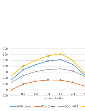
To extend these environments to the robust MDP setting (introduced in Section 2), we change the environment so that some model parameters (e.g., the mass of robot’s torso and ground friction) are randomly initialized in accordance with model parameter distributions. For the model parameter distribution, we prepare two types of distribution: continuous and discrete. For the continuous distribution, as in Rajeswaran et al. [24], we use a truncated Gaussian distribution, which follows the hyperparameters described in Table 2 in Appendices. For the discrete distribution, we use a Bernoulli distribution, which follows hyperparameters described in Table 2 in Appendices. We define the cost as the negative of the reward retrieved from the environment.

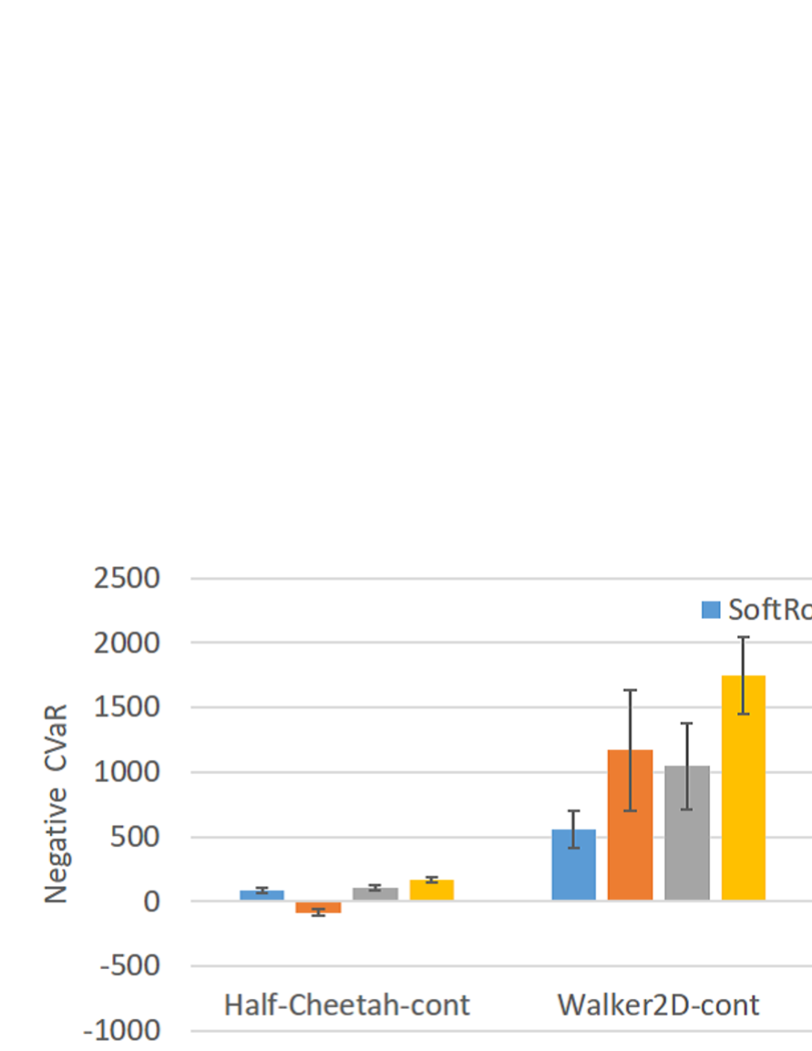
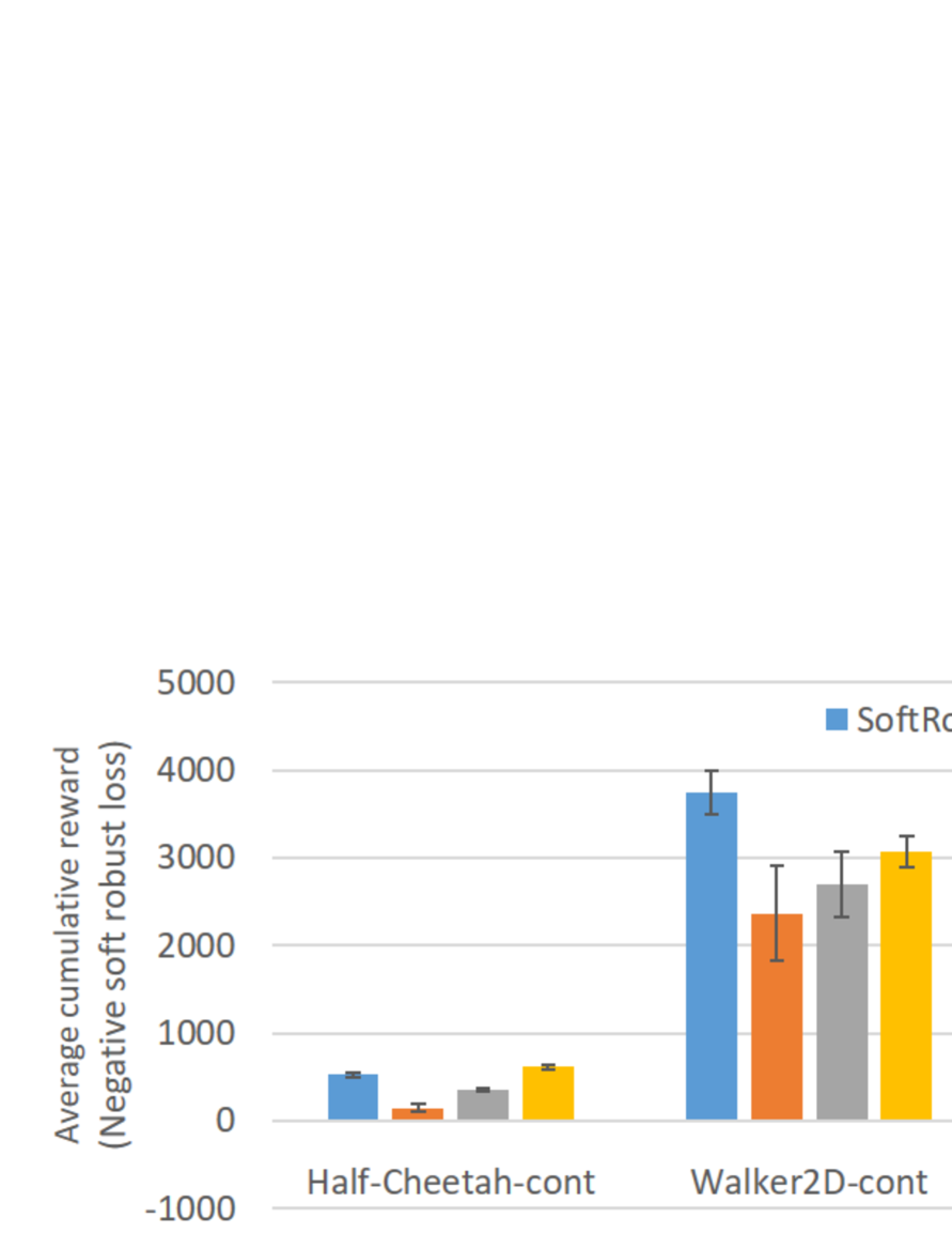
Regarding Q1, we find that OC3 can produce feasible options that keep CVaR lower than a given ζ𝜁\zeta (i.e., it satisfies the constraint in Eq. 2). The negative CVaR of each method in each environment is shown in Figure 1 (b). To focus on the non-trivial cases, we choose the best CVaR of the baselines (SoftRobust, WorstCase, and EOOpt-ϵitalic-ϵ\epsilon) and set ζ𝜁\zeta to it. For example, in the “Walker2D-disc” environment, the CVaR of WorstCase is used for ζ𝜁\zeta. The “OC3” in Figure 1 (b) is the negative CVaR with the given ζ𝜁\zeta. We can see that the negative CVaR score of OC3 is higher than the best negative CVaR score the baselines in each environment (i.e., the CVaR score of OC3 is lower than the given ζ𝜁\zeta). These results clearly demonstrate that our method successfully produces options satisfying the constraint. In addition, the numbers of successful learning trials for OC3 also support our claim (see Table 4 in Appendices).
Refer to caption
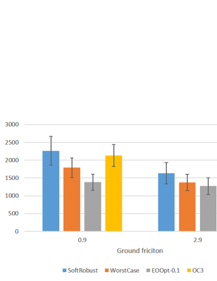
(a) The average-case performance: average cumulative reward (the negative of the soft robust loss Eq. 1)
Refer to caption
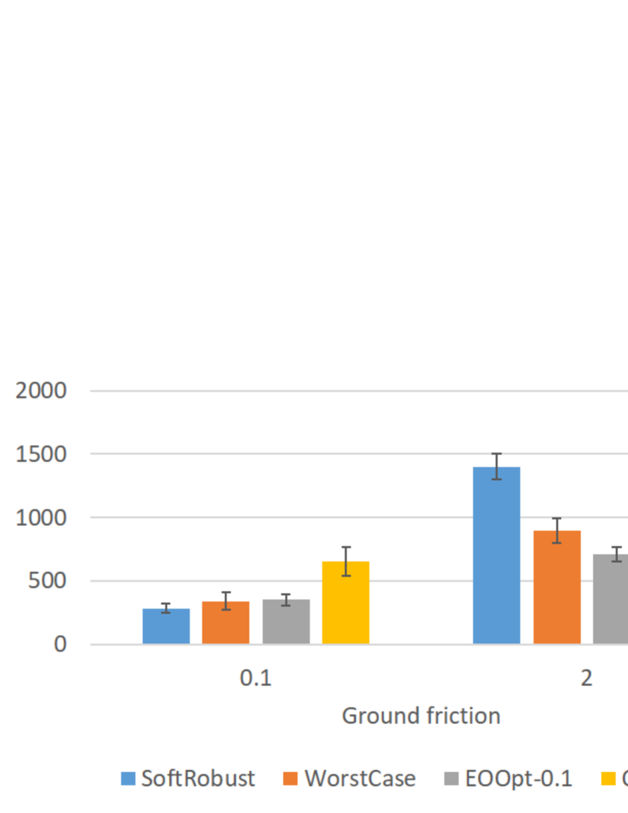
(b) The worst-case performance: negative CVaR with ϵ=0.1italic-ϵ0.1\epsilon=0.1. Here, CVaR is calculated as the average of losses included in the upper 10th percentile, and the negative of it is shown to the figure.
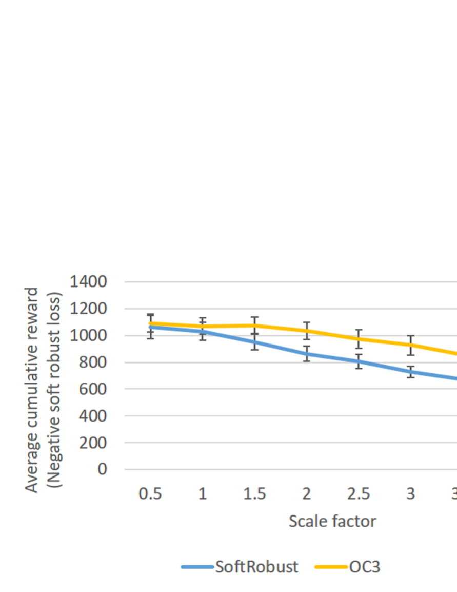
Figure 1: Comparison of methods in the environments. In (a), the vertical axis represents the average cumulative reward (the negative of the soft robust loss) of each method. In (b), the vertical axis represents the negative of CVaR of each method. In both (a) and (b), the horizontal axis represents environments where the methods are evaluated. The environments with suffix “-cont” are environments with the continuous model parameter distributions, and the environments with “-disc” are environments with the discrete model parameter distributions. The methods with high score values can be regarded as better. In addition, each score is averaged over 36 learning trials with different initial random seeds, and the 95%percent\% confidence interval is attached to the score.

In addition, regarding Q2, Figure 1 (b) also shows that the negative CVaRs of OC3 are higer than those of SoftRobust, in which the option is learned only to minimize the loss in the average case. Therefore, our method can be said to successfully produce options that work better in the worst case than the options learned only for the average case.

Regarding Q3, we compare the average-case (soft robust) loss (Eq. 1) of OC3 and those of worst-case methods (WorstCase and EOOpt-0.1). The soft robust loss of each method in each environment is shown in Figure 1 (a). We can see that the scores of OC3 are higher than those of WorstCase and EOOpt-0.1. These results indicate that our method can successfully produce options that work better in the average case than the options learned only for the worst case.

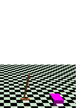
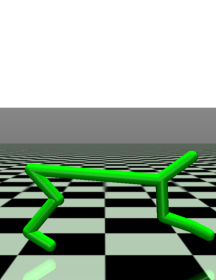
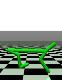
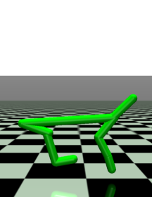
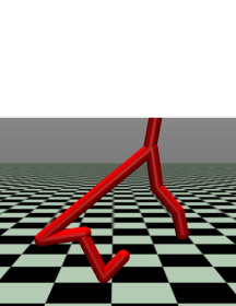
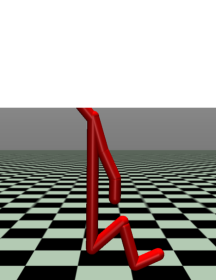
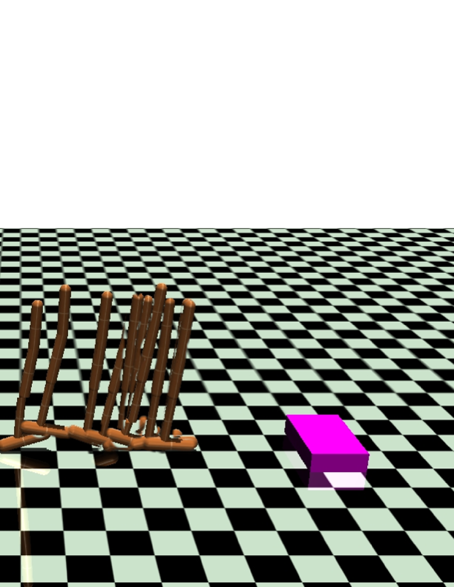
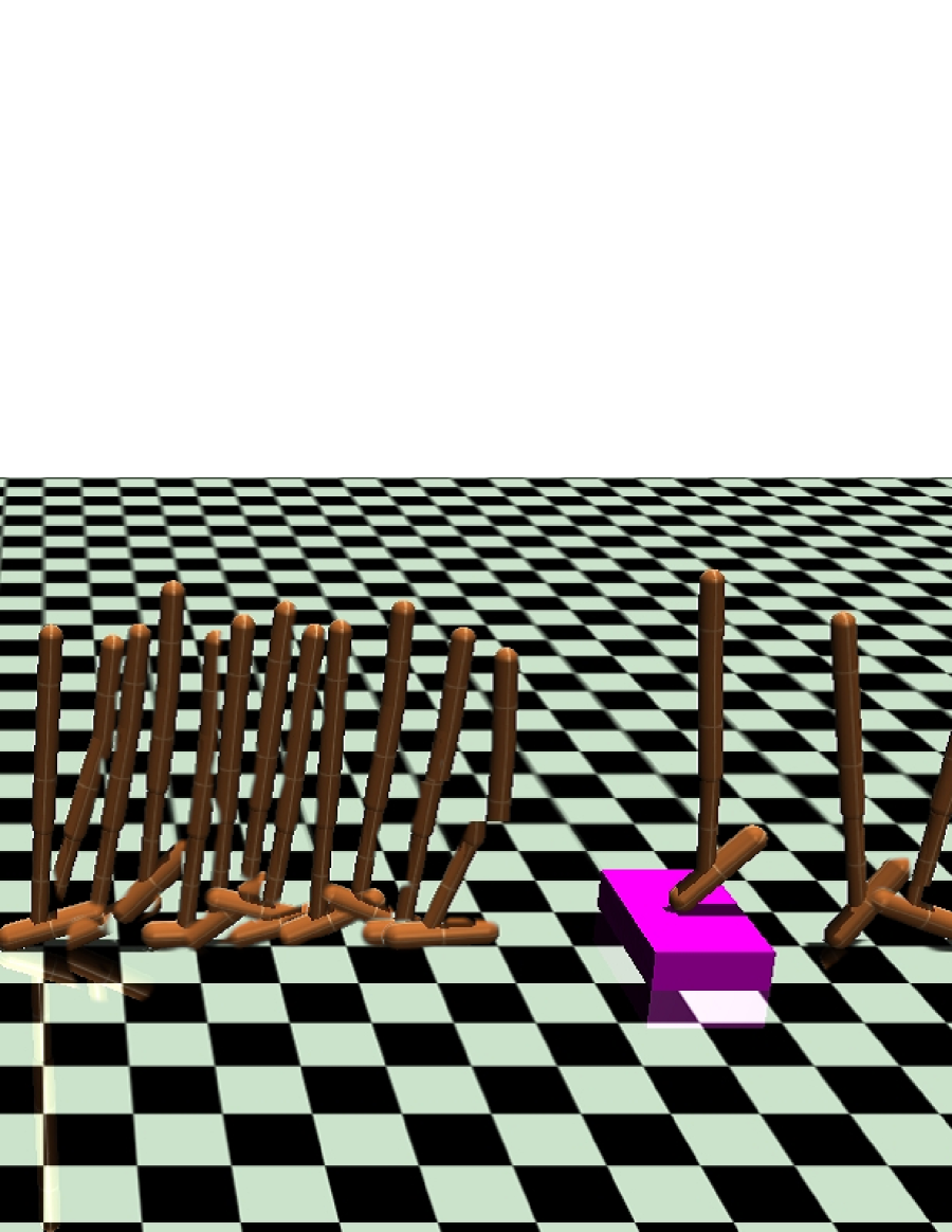
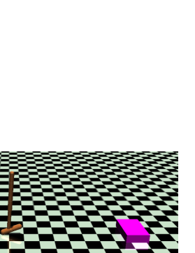
In the analysis of learned options, we find that OC3 and SoftRobust successfully produce options corresponding to decomposed skills required for solving the tasks in most environments. Especially, OC3 produces robust options. For example, in HopperIceBlock-disc, OC3 produces options corresponding to walking on slippery grounds and jumping onto a box (Figures 2). In addition, in HalfCheetah-disc, OC3 produces an option for running (highlighted in green in Figure 3) and an option for stabilizing the cheetah-bot’s body (highlighted in red in Figure 3), which is used mainly in the rare-case model parameter setups. Acquisition of such decomposed robust skills is useful when transferring to a different domain, and they can be also used for post-hoc human analysis and maintenance, which is an important advantage of option-based reinforcement learning over flat-policy reinforcement learning.
Refer to captionRefer to captionRefer to caption
Figure 2: Learned options in HopperIceBlock-disc. Left: the option for walking on the slippery ground. Right: the option for jumping onto the box.
Refer to captionRefer to captionRefer to captionRefer to caption
Figure 3: Learned options (shown in green when option 1 is taking the control and in red otherwise) in Halfcheetah-cont. Left: the case with an ordinary model parameter setup. Right: the case with a rare model parameters setup.

5 Related Work

Robust reinforcement learning (worst case): One of the main approaches for robust reinforcement learning is to learn policy by minimizing the expected loss in the worst case. “Worst case” is used in two different contexts: 1) the worst case under coherent uncertainty and 2) the worst case under parameter uncertainty. Coherent uncertainty is induced by the stochastic nature of MDPs (i.e., stochastic rewards and transition), whereas parameter uncertainty is induced by inaccurate environment models. For the worst case under coherent uncertainty, many robust reinforcement learning approaches have been proposed (e.g.,  [7, 8, 12]). Also, many robust reinforcement learning methods have been proposed for the worst case under parameter uncertainty [2, 14, 22, 23, 31, 34]. These works focus on learning robust “flat” policies (i.e., non-hierarchical policies), whereas we focus on learning robust “option” policies (i.e., hierarchical policies).

Robust reinforcement learning (CVaR): CVaR has previously been applied to reinforcement learning. Boda and Filar [4] used a dynamic programming approach to optimize CVaR. Morimura et al. [21] introduce CVaR to the exploration part of the SARSA algorithm. Rajeswaran et al. [24] introduced CVaR into model-based Bayesian reinforcement learning. Tamar and Chow  [6, 32] presented a policy gradient theorem for CVaR optimizing. These research efforts focus on learning robust flat policies, whereas we focus on learning robust options.

Learning robust options: Learning robust options is a relatively recent topic that not much work has addressed. Mankowitz et al. [19] are pioneers of this research topic. They proposed a robust option policy iteration to learn an option that minimizes the expected loss in the worst case under parameter uncertainty. Frans et al. [10] proposed a method to learn options that maximize the expected loss in the average case999Although their method is presented as a transfer learning method, their optimization objective is essentially equivalent to the “soft robust” objective in the robust reinforcement learning literature [9]. Thus, we regard their method as a robust option learning framework.. Both methods consider loss in either the worst or average case. Mankowitz’s method considers only the loss in the worst case, so the produced options are overly adapted to the worst case and does not work well in the average case. On the other hand, Frans’s method considers only the loss in the average case, so the produced options work poorly in the unconsidered case. In contrast to these methods, our method considers the losses in both the average and worst cases and thus can mitigate the aforementioned problems.

6 Conclusion

In this paper, we proposed a conditional value at risk (CVaR)-based method to learn options so that they 1) keep the expected loss lower than the given threshold (loss tolerance ζ𝜁\zeta) in the worst case and also 2) decrease the expected loss in the average case as much as possible. To achieve this, we extended Chow and Ghavamzadeh’s CVaR policy gradient method [6] to adapt robust Markov decision processes (robust MDPs) and then applied the extended method to learn robust options. For application, we derived a theorem for an option policy gradient for soft robust loss minimization [9]. We conducted experiments to evaluate our method in multi-joint robot control tasks. Experimental results show that our method produces options that 1) work better in the worst case than the options learned only to minimize the loss in the average case and 2) work better in the average case than the options learned only to minimize the loss in the worst case.

Although, in general, the model parameter distribution is not necessarily correct and thus needs to be updated to be more precise by reflecting observations retrieved from the real environment [24], our current method does not consider such model adaptation. One interesting direction for future works is to introduce this model adaptation, extending our method to adopt Bayes-Adaptive Markov decision processes [11].

References

  • Bacon et al. [2017] Bacon, P.-L., Harb, J., and Precup, D. The option-critic architecture. In Proc. AAAI, 2017.
  • Bagnell et al. [2001] Bagnell, J. A., Ng, A. Y., and Schneider, J. G. Solving uncertain Markov decision processes. Technical Report CMU-RITR-01-25, 2001.
  • Bertsekas [1999] Bertsekas, D. P. Nonlinear programming. Athena scientific Belmont, 1999.
  • Boda & Filar [2006] Boda, K. and Filar, J. A. Time consistent dynamic risk measures. Mathematical Methods of Operations Research, 63(1):169–186, 2006.
  • Brockman et al. [2016] Brockman, G., Cheung, V., Pettersson, L., Schneider, J., Schulman, J., Tang, J., and Zaremba, W. OpenAI Gym. arXiv:1606.01540 [cs.LG], 2016.
  • Chow & Ghavamzadeh [2014] Chow, Y. and Ghavamzadeh, M. Algorithms for CVaR optimization in MDPs. In Proc. NIPS, pp.  3509–3517, 2014.
  • Coraluppi & Marcus [1999a] Coraluppi, S. P. and Marcus, S. I. Risk-sensitive, minimax, and mixed risk-neutral / minimax control of markov decision processes. Stochastic Analysis, Control, Optimization and Applications: A Volume in Honor of W.H. Fleming, pp.  21–40, 1999a.
  • Coraluppi & Marcus [1999b] Coraluppi, S. P. and Marcus, S. I. Risk-sensitive and minimax control of discrete-time, finite-state markov decision processes. Automatica, 35(2):301–309, 1999b.
  • Derman et al. [2018] Derman, E., Mankowitz, D. J., Mann, T. A., and Mannor, S. Soft-Robust Actor-Critic Policy-Gradient. In Proc. UAI, 2018.
  • Frans et al. [2018] Frans, K., Ho, J., Chen, X., Abbeel, P., and Schulman, J. META LEARNING SHARED HIERARCHIES. In Proc. ICLR, 2018.
  • Ghavamzadeh et al. [2015] Ghavamzadeh, M., Mannor, S., Pineau, J., Tamar, A., et al. Bayesian reinforcement learning: A survey. Foundations and Trends in Machine Learning, 8(5-6):359–483, 2015.
  • Heger [1994] Heger, M. Consideration of risk in reinforcement learning. In Proc. ML, pp.  105–111. Elsevier, 1994.
  • Henderson et al. [2017] Henderson, P., Chang, W., Shkurti, F., Hansen, J., Meger, D., and Dudek, G. Benchmark environments for multitask learning in continuous domains. arXiv:1708.04352 [cs.AI], 2017.
  • Iyengar [2005] Iyengar, G. N. Robust dynamic programming. Mathematics of Operations Research, 30(2):257–280, 2005.
  • James et al. [2018] James, S., Wohlhart, P., Kalakrishnan, M., Kalashnikov, D., Irpan, A., Ibarz, J., Levine, S., Hadsell, R., and Bousmalis, K. Sim-to-Real via Sim-to-Sim: Data-efficient Robotic Grasping via Randomized-to-Canonical Adaptation Networks. arXiv:1812.07252 [cs.RO], 2018.
  • Klissarov et al. [2017] Klissarov, M., Bacon, P., Harb, J., and Precup, D. Learnings options end-to-end for continuous action tasks. ArXiv, 2017.
  • Konidaris & Barto [2009] Konidaris, G. and Barto, A. G. Skill discovery in continuous reinforcement learning domains using skill chaining. In Proc. NIPS, pp.  1015–1023, 2009.
  • Kulkarni et al. [2016] Kulkarni, T. D., Narasimhan, K., Saeedi, A., and Tenenbaum, J. Hierarchical deep reinforcement learning: Integrating temporal abstraction and intrinsic motivation. In Proc. NIPS, pp.  3675–3683, 2016.
  • Mankowitz et al. [2018] Mankowitz, D. J., Mann, T. A., Bacon, P.-L., Precup, D., and Mannor, S. Learning Robust Options. In Proc. AAAI, 2018.
  • McGovern & Barto [2001] McGovern, A. and Barto, A. G. Automatic discovery of subgoals in reinforcement learning using diverse density. Computer Science Department Faculty Publication Series, 8, 2001.
  • Morimura et al. [2010] Morimura, T., Sugiyama, M., Kashima, H., Hachiya, H., and Tanaka, T. Nonparametric return distribution approximation for reinforcement learning. In Proc. ICML, pp.  799–806, 2010.
  • Nilim & El Ghaoui [2005] Nilim, A. and El Ghaoui, L. Robust control of markov decision processes with uncertain transition matrices. Operations Research, 53(5):780–798, 2005.
  • Pinto et al. [2017] Pinto, L., Davidson, J., Sukthankar, R., and Gupta, A. Robust adversarial reinforcement learning. In Proc. ICML, pp.  2817–2826, 2017.
  • Rajeswaran et al. [2017] Rajeswaran, A., Ghotra, S., Levine, S., and Ravindran, B. EPOpt: Learning Robust Neural Network Policies Using Model Ensembles. In Proc. ICLR, 2017.
  • Rockafellar & Uryasev [2002] Rockafellar, R. T. and Uryasev, S. Conditional value-at-risk for general loss distributions. Journal of banking & finance, 26(7):1443–1471, 2002.
  • Schulman et al. [2016] Schulman, J., Moritz, P., Levine, S., Jordan, M., and Abbeel, P. High-dimensional continuous control using generalized advantage estimation. In Proc. ICLR, 2016.
  • Schulman et al. [2017] Schulman, J., Wolski, F., Dhariwal, P., Radford, A., and Klimov, O. Proximal policy optimization algorithms. arXiv:1707.06347 [cs.LG], 2017.
  • Silver & Ciosek [2012] Silver, D. and Ciosek, K. Compositional planning using optimal option models. In Proc. ICML, 2012.
  • Stolle & Precup [2002] Stolle, M. and Precup, D. Learning options in reinforcement learning. In Proc. SARA, pp.  212–223. Springer, 2002.
  • Sutton et al. [1999] Sutton, R. S., Precup, D., and Singh, S. Between mdps and semi-mdps: A framework for temporal abstraction in reinforcement learning. Artificial intelligence, 112(1-2):181–211, 1999.
  • Tamar et al. [2014] Tamar, A., Mannor, S., and Xu, H. Scaling up robust mdps using function approximation. In Proc. ICML, pp.  181–189, 2014.
  • Tamar et al. [2015] Tamar, A., Glassner, Y., and Mannor, S. Optimizing the CVaR via Sampling. In Proc. AAAI, pp.  2993–2999, 2015.
  • Wawrzyński [2009] Wawrzyński, P. Real-time reinforcement learning by sequential actor–critics and experience replay. Neural Networks, 22(10):1484–1497, 2009.
  • Wiesemann et al. [2013] Wiesemann, W., Kuhn, D., and Rustem, B. Robust markov decision processes. Mathematics of Operations Research, 38(1):153–183, 2013.
  • Xu & Mannor [2010] Xu, H. and Mannor, S. Distributionally robust markov decision processes. In Proc. NIPS, pp.  2505–2513, 2010.

Appendices

Algorithmic Representation of EOOpt-ϵitalic-ϵ\epsilon

The outline of EOOpt-ϵitalic-ϵ\epsilon is summarized in Algorithm 2. Here 𝒞(τk)=t=0Tγtct(k)𝒞subscript𝜏𝑘superscriptsubscript𝑡0𝑇superscript𝛾𝑡superscriptsubscript𝑐𝑡𝑘\mathcal{C}(\tau_{k})=\sum_{t=0}^{T}\gamma^{t}c_{t}^{(k)} is a loss in the trajectory k𝑘k and ct(k)superscriptsubscript𝑐𝑡𝑘c_{t}^{(k)} is a cost at the t𝑡t-th turn in k𝑘k. PPOCUpdateParams returns the updated parameters on the basis of given trajectories and parameters. This functions is identical to the advantage estimation and parameter update part of Algorithm 1 in Klissarov et al. [16].

Algorithm 2 EOOpt-ϵitalic-ϵ\epsilon
0:  θπω,0subscript𝜃subscript𝜋𝜔0\theta_{\pi_{\omega},0}, θβω,0subscript𝜃subscript𝛽𝜔0\theta_{\beta_{\omega},0}, θπΩ,0subscript𝜃subscript𝜋Ω0\theta_{\pi_{\Omega},0}, Niter,Nepi,ϵ,Ωsubscript𝑁𝑖𝑡𝑒𝑟subscript𝑁𝑒𝑝𝑖italic-ϵΩN_{iter},N_{epi},\epsilon,\Omega
1:  for iteration i=0,1,,Niter𝑖01subscript𝑁𝑖𝑡𝑒𝑟i=0,1,...,N_{iter} do
2:     for k=0,1,,Nepi𝑘01subscript𝑁𝑒𝑝𝑖k=0,1,...,N_{epi} do
3:        sample model parameters pksimilar-tosubscript𝑝𝑘p_{k}\sim\mathbb{P}
4:        sample a trajectory τk={st,ωt,at,ct,st+1}t=0T1subscript𝜏𝑘superscriptsubscriptsubscript𝑠𝑡subscript𝜔𝑡subscript𝑎𝑡subscript𝑐𝑡subscript𝑠𝑡1𝑡0𝑇1\tau_{k}=\left\{s_{t},\omega_{t},a_{t},c_{t},s_{t+1}\right\}_{t=0}^{T-1} from parameterized MDPs S,A,,γ,Tpk,0𝑆𝐴𝛾subscript𝑇subscript𝑝𝑘subscript0\left\langle S,A,\mathbb{C},\gamma,T_{p_{k}},\mathbb{P}_{0}\right\rangle using option policies (πωsubscript𝜋𝜔\pi_{\omega}, βωsubscript𝛽𝜔\beta_{\omega}, and πΩsubscript𝜋Ω\pi_{\Omega}) with θπω,isubscript𝜃subscript𝜋𝜔𝑖\theta_{\pi_{\omega},i}, θβω,isubscript𝜃subscript𝛽𝜔𝑖\theta_{\beta_{\omega},i}, and θπΩ,isubscript𝜃subscript𝜋Ω𝑖\theta_{\pi_{\Omega},i}.
5:     end for
6:     compute Qϵ=subscript𝑄italic-ϵabsentQ_{\epsilon}= upper ϵitalic-ϵ\epsilon percentile of {𝒞(τk)}k=0Nepisuperscriptsubscript𝒞subscript𝜏𝑘𝑘0subscript𝑁𝑒𝑝𝑖\{\mathcal{C}(\tau_{k})\}_{k=0}^{N_{epi}}
7:     select sub-set 𝕋={τk|𝒞(τk)Qϵ}𝕋conditional-setsubscript𝜏𝑘𝒞subscript𝜏𝑘subscript𝑄italic-ϵ\mathbb{T}=\{\tau_{k}|\mathcal{C}(\tau_{k})\geq Q_{\epsilon}\}
8:     θπω,i+1subscript𝜃subscript𝜋𝜔𝑖1\theta_{\pi_{\omega},i+1}, θβω,i+1subscript𝜃subscript𝛽𝜔𝑖1\theta_{\beta_{\omega},i+1}, θπΩ,i+1PPOCUpdateParams(𝕋,θπω,i\theta_{\pi_{\Omega},i+1}\leftarrow\text{PPOCUpdateParams}(\mathbb{T},\theta_{\pi_{\omega},i}, θβω,isubscript𝜃subscript𝛽𝜔𝑖\theta_{\beta_{\omega},i}, θπΩ,i)\theta_{\pi_{\Omega},i})
9:  end for

Decompositionability of 𝔼𝒞,p[max(0,𝒞v)]subscript𝔼𝒞𝑝delimited-[]0𝒞𝑣\mathbb{E}_{\mathcal{C},p}\left[\max(0,\mathcal{C}-v)\right] with Respect to p𝑝p

Corollary 1 (Decompositionability of 𝔼𝒞,p[max(0,𝒞v)]subscript𝔼𝒞𝑝delimited-[]0𝒞𝑣\mathbb{E}_{\mathcal{C},p}\left[\max(0,\mathcal{C}-v)\right] with Respect to p𝑝p).
𝔼𝒞,p[max(0,𝒞v)]=p(p)𝔼𝒞[max(0,𝒞v)p].subscript𝔼𝒞𝑝delimited-[]0𝒞𝑣subscript𝑝𝑝subscript𝔼𝒞delimited-[]conditional0𝒞𝑣𝑝\displaystyle\mathbb{E}_{\mathcal{C},p}\left[\max(0,\mathcal{C}-v)\right]=\sum_{p}\mathbb{P}(p)\mathbb{E}_{\mathcal{C}}\left[\max(0,\mathcal{C}-v)\mid p\right].
Proof.

By letting (𝒞,p)𝒞𝑝\mathbb{P}\left(\mathcal{C},p\right) be a joint distribution of the loss and the model parameter and (𝒞p)conditional𝒞𝑝\mathbb{P}\left(\mathcal{C}\mid p\right) be the conditional distribution of the loss, 𝔼𝒞,p[max(0,𝒞v)]subscript𝔼𝒞𝑝delimited-[]0𝒞𝑣\mathbb{E}_{\mathcal{C},p}\left[\max(0,\mathcal{C}-v)\right] can be transformed as

𝔼𝒞,p[max(0,𝒞v)]subscript𝔼𝒞𝑝delimited-[]0𝒞𝑣\displaystyle\mathbb{E}_{\mathcal{C},p}\left[\max(0,\mathcal{C}-v)\right] =\displaystyle= 𝒞p(𝒞,p)max(0,𝒞v)subscript𝒞subscript𝑝𝒞𝑝0𝒞𝑣\displaystyle\sum_{\mathcal{C}}\sum_{p}\mathbb{P}\left(\mathcal{C},p\right)\max(0,\mathcal{C}-v) (20)
=\displaystyle= p(p)𝒞(𝒞p)max(0,𝒞v)subscript𝑝𝑝subscript𝒞conditional𝒞𝑝0𝒞𝑣\displaystyle\sum_{p}\mathbb{P}(p)\sum_{\mathcal{C}}\mathbb{P}\left(\mathcal{C}\mid p\right)\max(0,\mathcal{C}-v)
=\displaystyle= p(p)𝔼𝒞[max(0,𝒞v)p].subscript𝑝𝑝subscript𝔼𝒞delimited-[]conditional0𝒞𝑣𝑝\displaystyle\sum_{p}\mathbb{P}(p)\mathbb{E}_{\mathcal{C}}\left[\max(0,\mathcal{C}-v)\mid p\right].

Derivation of Option Policy Gradient Theorems for Soft Robust Loss

Here, we derive option policy gradient theorems for soft robust loss p(p)𝔼𝒞[𝒞p]subscript𝑝𝑝subscript𝔼𝒞delimited-[]conditional𝒞𝑝\sum_{p}\mathbb{P}(p)\mathbb{E}_{\mathcal{C}}\left[\mathcal{C}\mid p\right], where 𝔼𝒞[𝒞|p]subscript𝔼𝒞delimited-[]conditional𝒞𝑝\mathbb{E}_{\mathcal{C}}\left[\mathcal{C}~{}|~{}p\right] is the expected loss on the general class of parameterized MDPs S,A,,γ,Tp,0𝑆𝐴𝛾subscript𝑇𝑝subscript0\langle S,A,\mathbb{C},\gamma,T_{p},\mathbb{P}_{0}\rangle101010 For derivation on the general case, we consider the general class of parameterized MDPs, to which the parameterized MDP in Section 2 and the augmented parameterized MDP in Section 3.1 belong. , in which the transition probability is parameterized by pP𝑝𝑃p\in P. In addition, (p)𝑝\mathbb{P}(p) is a distribution of p𝑝p. For convenience, in the latter part, we use (sSsS,aA,p)\mathbb{P}(s^{\prime}\in S\mid s\in S,a\in A,p) to refer to the parameterized transition function (i.e., Tpsubscript𝑇𝑝T_{p}). We make the rectangularity assumption on P𝑃P and (p)𝑝\mathbb{P}(p). That is, P𝑃P is assumed to be structured as a Cartesian product sSPssubscripttensor-product𝑠𝑆subscript𝑃𝑠\bigotimes_{s\in S}P_{s}, and \mathbb{P} is also assumed to be structured as a Cartesian product sSs(psPs)subscripttensor-product𝑠𝑆subscript𝑠subscript𝑝𝑠subscript𝑃𝑠\bigotimes_{s\in S}\mathbb{P}_{s}(p_{s}\in P_{s}) 111111More explicitly, P𝑃P and (p)𝑝\mathbb{P}(p) are defined as t0sSPs,tsuperscriptsubscripttensor-product𝑡0subscripttensor-product𝑠𝑆subscript𝑃𝑠𝑡\bigotimes_{t\in 0}^{\infty}\bigotimes_{s\in S}P_{s,t} and t0sSs,t(ps,tPs,t)superscriptsubscripttensor-product𝑡0subscripttensor-product𝑠𝑆subscript𝑠𝑡subscript𝑝𝑠𝑡subscript𝑃𝑠𝑡\bigotimes_{t\in 0}^{\infty}\bigotimes_{s\in S}\mathbb{P}_{s,t}(p_{s,t}\in P_{s,t}), where Ps,t=Pssubscript𝑃𝑠𝑡subscript𝑃𝑠P_{s,t}=P_{s} and Ps,t(psPs,t)=Ps(psPs)subscript𝑃𝑠𝑡subscript𝑝𝑠subscript𝑃𝑠𝑡subscript𝑃𝑠subscript𝑝𝑠subscript𝑃𝑠{P}_{s,t}(p_{s}\in P_{s,t})={P}_{s}(p_{s}\in P_{s}), respectively. .

To prepare for the derivation, we define functions and variables. First, considering the definition of value functions in Bacon et al. [1], we define value functions in (the general class of) the parameterized MDP:

QΩ(s,ω,ps)subscript𝑄Ω𝑠𝜔subscript𝑝𝑠\displaystyle Q_{\Omega}(s,\omega,p_{s}) =\displaystyle= aπω(as)Qω(s,ω,a,ps),subscript𝑎subscript𝜋𝜔conditional𝑎𝑠subscript𝑄𝜔𝑠𝜔𝑎subscript𝑝𝑠\displaystyle\sum_{a}\pi_{\omega}(a\mid s)Q_{\omega}(s,\omega,a,p_{s}), (21)
Qω(s,ω,a,ps)subscript𝑄𝜔𝑠𝜔𝑎subscript𝑝𝑠\displaystyle Q_{\omega}(s,\omega,a,p_{s}) =\displaystyle= (s,a)+γs(ss,a,ps)Qβ(s,ω,ps),𝑠𝑎𝛾subscriptsuperscript𝑠conditionalsuperscript𝑠𝑠𝑎subscript𝑝𝑠subscript𝑄𝛽superscript𝑠𝜔subscript𝑝𝑠\displaystyle\mathbb{C}(s,a)+\gamma\sum_{s^{\prime}}\mathbb{P}\left(s^{\prime}\mid s,a,p_{s}\right)Q_{\beta}\left(s^{\prime},\omega,p_{s}\right), (22)
Qβ(s,ω,ps)subscript𝑄𝛽𝑠𝜔subscript𝑝𝑠\displaystyle Q_{\beta}(s,\omega,p_{s}) =\displaystyle= (1βω(s))QΩ(s,ω,ps)+βω(s)VΩ(s,ps),1subscript𝛽𝜔𝑠subscript𝑄Ω𝑠𝜔subscript𝑝𝑠subscript𝛽𝜔𝑠subscript𝑉Ω𝑠subscript𝑝𝑠\displaystyle(1-\beta_{\omega}(s))Q_{\Omega}(s,\omega,p_{s})+\beta_{\omega}(s)V_{\Omega}(s,p_{s}), (23)
VΩ(s,ps)subscript𝑉Ω𝑠subscript𝑝𝑠\displaystyle V_{\Omega}(s,p_{s}) =\displaystyle= ωπΩ(ωs)QΩ(s,ω,ps).subscript𝜔subscript𝜋Ωconditional𝜔𝑠subscript𝑄Ω𝑠𝜔subscript𝑝𝑠\displaystyle\sum_{\omega}\pi_{\Omega}(\omega\mid s)Q_{\Omega}(s,\omega,p_{s}). (24)

Note that by fixing pssubscript𝑝𝑠p_{s} to a constant value, these value functions can be seen as identical to those in Bacon et al. [1].

Second, for convenience, we define the discounted probabilities to (st+1,ωt+1)subscript𝑠𝑡1subscript𝜔𝑡1(s_{t+1},\omega_{t+1}) from (st,ωt)subscript𝑠𝑡subscript𝜔𝑡(s_{t},\omega_{t}):

γ(1)(st+1,ωt+1st,ωt)subscriptsuperscript1𝛾subscript𝑠𝑡1conditionalsubscript𝜔𝑡1subscript𝑠𝑡subscript𝜔𝑡\displaystyle\mathbb{P}^{(1)}_{\gamma}(s_{t+1},\omega_{t+1}\mid s_{t},\omega_{t}) =\displaystyle= aπω(ast)γpstst(pst)(st+1st,a,pst)subscript𝑎subscript𝜋𝜔conditional𝑎subscript𝑠𝑡𝛾subscriptsubscript𝑝subscript𝑠𝑡subscriptsubscript𝑠𝑡subscript𝑝subscript𝑠𝑡conditionalsubscript𝑠𝑡1subscript𝑠𝑡𝑎subscript𝑝subscript𝑠𝑡\displaystyle\sum_{a}\pi_{\omega}(a\mid s_{t})\gamma\sum_{p_{s_{t}}}\mathbb{P}_{s_{t}}(p_{s_{t}})\mathbb{P}\left(s_{t+1}\mid s_{t},a,p_{s_{t}}\right) (25)
((1βω(st+1))1(ωt+1=ωt)+βω(st+1)πΩ(ωt+1|st+1)),absent1subscript𝛽𝜔subscript𝑠𝑡11subscript𝜔𝑡1subscript𝜔𝑡subscript𝛽𝜔subscript𝑠𝑡1subscript𝜋Ωconditionalsubscript𝜔𝑡1subscript𝑠𝑡1\displaystyle\cdot\left((1-\beta_{\omega}(s_{t+1}))\textbf{1}(\omega_{t+1}=\omega_{t})+\beta_{\omega}(s_{t+1})\pi_{\Omega}(\omega_{t+1}|s_{t+1})\right),
γ(k)(st+k,ωt+kst,ωt)subscriptsuperscript𝑘𝛾subscript𝑠𝑡𝑘conditionalsubscript𝜔𝑡𝑘subscript𝑠𝑡subscript𝜔𝑡\displaystyle\mathbb{P}^{(k)}_{\gamma}(s_{t+k},\omega_{t+k}\mid s_{t},\omega_{t}) =\displaystyle= st+1ωt+1γ(1)(st+1,ωt+1st,ωt)γ(k1)(st+k,ωt+kst+1,ωt+1).subscriptsubscript𝑠𝑡1subscriptsubscript𝜔𝑡1superscriptsubscript𝛾1subscript𝑠𝑡1conditionalsubscript𝜔𝑡1subscript𝑠𝑡subscript𝜔𝑡subscriptsuperscript𝑘1𝛾subscript𝑠𝑡𝑘conditionalsubscript𝜔𝑡𝑘subscript𝑠𝑡1subscript𝜔𝑡1\displaystyle\sum_{s_{t+1}}\sum_{\omega_{t+1}}\mathbb{P}_{\gamma}^{(1)}(s_{t+1},\omega_{t+1}\mid s_{t},\omega_{t})\mathbb{P}^{(k-1)}_{\gamma}(s_{t+k},\omega_{t+k}\mid s_{t+1},\omega_{t+1}). (26)

Similar discounted probabilities are also introduced in Bacon et al. [1]. Ours (Eq. 25 and Eq. 26) are different from theirs in that the transition function is averaged over the model parameter (i.e., pstst(pst)(st+1st,a,pst)=𝔼ps[(ss,a,ps)]subscriptsubscript𝑝subscript𝑠𝑡subscriptsubscript𝑠𝑡subscript𝑝subscript𝑠𝑡conditionalsubscript𝑠𝑡1subscript𝑠𝑡𝑎subscript𝑝subscript𝑠𝑡subscript𝔼subscript𝑝𝑠delimited-[]conditionalsuperscript𝑠𝑠𝑎subscript𝑝𝑠\sum_{p_{s_{t}}}\mathbb{P}_{s_{t}}(p_{s_{t}})\mathbb{P}(s_{t+1}\mid s_{t},a,p_{s_{t}})=\mathbb{E}_{p_{s}}\left[\mathbb{P}(s^{\prime}\mid s,a,p_{s})\right]).

In addition, by using the rectangularity assumption on (p)𝑝\mathbb{P}(p), we introduce the equation which represents the state-wise independence of the model parameter distribution121212This state-wise independence is essentially the same as that introduced in the proof of Proposition 3.2 in Derman et al. [9]. :

pstPstst(pst)st+1(st+1|st,at,pst)QΩ(st+1,ωt,pst)subscriptsubscript𝑝subscript𝑠𝑡subscript𝑃subscript𝑠𝑡subscriptsubscript𝑠𝑡subscript𝑝subscript𝑠𝑡subscriptsubscript𝑠𝑡1conditionalsubscript𝑠𝑡1subscript𝑠𝑡subscript𝑎𝑡subscript𝑝subscript𝑠𝑡subscript𝑄Ωsubscript𝑠𝑡1subscript𝜔𝑡subscript𝑝subscript𝑠𝑡\displaystyle\sum_{p_{s_{t}}\in P_{s_{t}}}\mathbb{P}_{s_{t}}(p_{s_{t}})\sum_{s_{t+1}}\mathbb{P}\left(\left.s_{t+1}~{}\right|s_{t},a_{t},p_{s_{t}}\right)Q_{\Omega}(s_{t+1},\omega_{t},p_{s_{t}})
=st+1(pstst(pst)(st+1|st,at,pst))(pst+1Pst+1st+1(pst+1)QΩ(st+1,ωt,pst+1)).absentsubscriptsubscript𝑠𝑡1subscriptsubscript𝑝subscript𝑠𝑡subscriptsubscript𝑠𝑡subscript𝑝subscript𝑠𝑡conditionalsubscript𝑠𝑡1subscript𝑠𝑡subscript𝑎𝑡subscript𝑝subscript𝑠𝑡subscriptsubscript𝑝subscript𝑠𝑡1subscript𝑃subscript𝑠𝑡1subscriptsubscript𝑠𝑡1subscript𝑝subscript𝑠𝑡1subscript𝑄Ωsubscript𝑠𝑡1subscript𝜔𝑡subscript𝑝subscript𝑠𝑡1\displaystyle~{}~{}~{}~{}=\sum_{s_{t+1}}\left(\sum_{p_{s_{t}}}\mathbb{P}_{s_{t}}(p_{s_{t}})\mathbb{P}\left(\left.s_{t+1}~{}\right|s_{t},a_{t},p_{s_{t}}\right)\right)\left(\sum_{p_{s_{t+1}}\in P_{s_{t+1}}}\mathbb{P}_{s_{t+1}}\left(p_{s_{t+1}}\right)Q_{\Omega}\left(s_{t+1},\omega_{t},p_{s_{t+1}}\right)\right). (27)

Now, we start the derivation of option policy gradient theorems for soft robust loss. We derive the gradient theorem in a similar manner to Bacon et al. [1].

Theorem 1 (Policy over options gradient theorem for soft robust loss).

Given a set of options with a stochastic policy over options πΩsubscript𝜋Ω\pi_{\Omega} that are differentiable in their parameters θπΩsubscript𝜃subscript𝜋Ω\theta_{\pi_{\Omega}}, the gradient of the soft robust loss with respect to θπΩsubscript𝜃subscript𝜋Ω\theta_{\pi_{\Omega}} and initial condition (s0,ω0)subscript𝑠0subscript𝜔0(s_{0},\omega_{0}) is:

pss(ps)QΩ(s,ω,ps)θπΩ=sd¯Ω(ss0,ω0)ωπΩ(ω|s)θπΩQ¯Ω(s,ω),subscriptsubscript𝑝𝑠subscript𝑠subscript𝑝𝑠subscript𝑄Ω𝑠𝜔subscript𝑝𝑠subscript𝜃subscript𝜋Ωsubscript𝑠subscript¯𝑑Ωconditional𝑠subscript𝑠0subscript𝜔0subscript𝜔subscript𝜋Ωconditional𝜔𝑠subscript𝜃subscript𝜋Ωsubscript¯𝑄Ω𝑠𝜔\displaystyle\sum_{p_{s}}\mathbb{P}_{s}(p_{s})\frac{\partial Q_{\Omega}(s,\omega,p_{s})}{\partial\theta_{\pi_{\Omega}}}=\sum_{s}\overline{d}_{\Omega}(s\mid s_{0},\omega_{0})\sum_{\omega}\frac{\partial\pi_{\Omega}(\omega|s)}{\partial\theta_{\pi_{\Omega}}}\overline{Q}_{\Omega}(s,\omega),

where d¯Ω(ss0,ω0)subscript¯𝑑Ωconditional𝑠subscript𝑠0subscript𝜔0\overline{d}_{\Omega}(s\mid s_{0},\omega_{0}) is a discounted weighting of option pairs along trajectories from (s0,ω0)subscript𝑠0subscript𝜔0(s_{0},\omega_{0}): d¯Ω(ss0,ω0)=k=0γ(k)(ss0,ω0)subscript¯𝑑Ωconditional𝑠subscript𝑠0subscript𝜔0superscriptsubscript𝑘0subscriptsuperscript𝑘𝛾conditional𝑠subscript𝑠0subscript𝜔0\overline{d}_{\Omega}(s\mid s_{0},\omega_{0})=\sum_{k=0}^{\infty}\mathbb{P}^{(k)}_{\gamma}(s\mid s_{0},\omega_{0}), and Q¯Ω(s,ω)subscript¯𝑄Ω𝑠𝜔\overline{Q}_{\Omega}(s,\omega) is the average option value function: Q¯Ω(s,ω)=pss(ps)QΩ(s,ω,ps)subscript¯𝑄Ω𝑠𝜔subscriptsubscript𝑝𝑠subscript𝑠subscript𝑝𝑠subscript𝑄Ω𝑠𝜔subscript𝑝𝑠\overline{Q}_{\Omega}(s,\omega)=\sum_{p_{s}}\mathbb{P}_{s}(p_{s})Q_{\Omega}(s,\omega,p_{s}). By letting 𝔼ps[(ss,a,ps)]subscript𝔼subscript𝑝𝑠delimited-[]conditionalsuperscript𝑠𝑠𝑎subscript𝑝𝑠\mathbb{E}_{p_{s}}\left[\mathbb{P}(s^{\prime}\mid s,a,p_{s})\right] be a transition probability, the trajectories can be regarded as ones generated from the general class of the average parameterized MDPs S,A,,γ,𝔼ps[(ss,a,ps)],0𝑆𝐴𝛾subscript𝔼subscript𝑝𝑠delimited-[]conditionalsuperscript𝑠𝑠𝑎subscript𝑝𝑠subscript0\left\langle S,A,\mathbb{C},\gamma,\mathbb{E}_{p_{s}}\left[\mathbb{P}(s^{\prime}\mid s,a,p_{s})\right],\mathbb{P}_{0}\right\rangle.

Proof.

The gradient of Eq. 21 and Eq. 23 with respect to θπΩsubscript𝜃subscript𝜋Ω\theta_{\pi_{\Omega}} can be transformed as

QΩ(s,ω,ps)θπΩ=aπω(as)sγ(ss,a,ps)Qβ(ω,s,ps)θπΩ,subscript𝑄Ω𝑠𝜔subscript𝑝𝑠subscript𝜃subscript𝜋Ωsubscript𝑎subscript𝜋𝜔conditional𝑎𝑠subscriptsuperscript𝑠𝛾conditionalsuperscript𝑠𝑠𝑎subscript𝑝𝑠subscript𝑄𝛽𝜔superscript𝑠subscript𝑝𝑠subscript𝜃subscript𝜋Ω\displaystyle\frac{\partial Q_{\Omega}(s,\omega,p_{s})}{\partial\theta_{\pi_{\Omega}}}=\sum_{a}\pi_{\omega}(a\mid s)\sum_{s^{\prime}}\gamma\mathbb{P}(s^{\prime}\mid s,a,p_{s})\frac{\partial Q_{\beta}(\omega,s^{\prime},p_{s})}{\partial\theta_{\pi_{\Omega}}}, (28)
Qβ(s,ω,ps)θπΩ=(1βω(s))QΩ(s,ω,ps)θπΩ+ββ(s)VΩ(s,ps)θπΩsubscript𝑄𝛽𝑠𝜔subscript𝑝𝑠subscript𝜃subscript𝜋Ω1subscript𝛽𝜔superscript𝑠subscript𝑄Ωsuperscript𝑠𝜔subscript𝑝𝑠subscript𝜃subscript𝜋Ωsubscript𝛽𝛽superscript𝑠subscript𝑉Ωsuperscript𝑠subscript𝑝𝑠subscript𝜃subscript𝜋Ω\displaystyle\frac{\partial Q_{\beta}(s,\omega,p_{s})}{\partial\theta_{\pi_{\Omega}}}=(1-\beta_{\omega}(s^{\prime}))\frac{\partial Q_{\Omega}(s^{\prime},\omega,p_{s})}{\partial\theta_{\pi_{\Omega}}}+\beta_{\beta}(s^{\prime})\frac{\partial V_{\Omega}(s^{\prime},p_{s})}{\partial\theta_{\pi_{\Omega}}}
=(1βω(s))QΩ(s,ω,ps)θπΩ+βω(s)ωπΩ(ω|s)θπΩQΩ(s,ω,ps)absent1subscript𝛽𝜔superscript𝑠subscript𝑄Ωsuperscript𝑠𝜔subscript𝑝𝑠subscript𝜃subscript𝜋Ωsubscript𝛽𝜔superscript𝑠subscriptsuperscript𝜔subscript𝜋Ωconditionalsuperscript𝜔superscript𝑠subscript𝜃subscript𝜋Ωsubscript𝑄Ωsuperscript𝑠superscript𝜔subscript𝑝𝑠\displaystyle=(1-\beta_{\omega}(s^{\prime}))\frac{\partial Q_{\Omega}(s^{\prime},\omega,p_{s})}{\partial\theta_{\pi_{\Omega}}}+\beta_{\omega}(s^{\prime})\sum_{\omega^{\prime}}\frac{\partial\pi_{\Omega}(\omega^{\prime}|s^{\prime})}{\partial\theta_{\pi_{\Omega}}}Q_{\Omega}(s^{\prime},\omega^{\prime},p_{s})
+βω(s)ωπΩ(ω|s)QΩ(s,ω,ps)θπΩsubscript𝛽𝜔superscript𝑠subscriptsuperscript𝜔subscript𝜋Ωconditionalsuperscript𝜔superscript𝑠subscript𝑄Ωsuperscript𝑠superscript𝜔subscript𝑝𝑠subscript𝜃subscript𝜋Ω\displaystyle~{}~{}~{}~{}+\beta_{\omega}(s^{\prime})\sum_{\omega^{\prime}}\pi_{\Omega}(\omega^{\prime}|s^{\prime})\frac{\partial Q_{\Omega}(s^{\prime},\omega^{\prime},p_{s})}{\partial\theta_{\pi_{\Omega}}}
=βω(s)ωπΩ(ω|s)θπΩQΩ(s,ω,ps)absentsubscript𝛽𝜔superscript𝑠subscriptsuperscript𝜔subscript𝜋Ωconditionalsuperscript𝜔superscript𝑠subscript𝜃subscript𝜋Ωsubscript𝑄Ωsuperscript𝑠superscript𝜔subscript𝑝𝑠\displaystyle=\beta_{\omega}(s^{\prime})\sum_{\omega^{\prime}}\frac{\partial\pi_{\Omega}(\omega^{\prime}|s^{\prime})}{\partial\theta_{\pi_{\Omega}}}Q_{\Omega}(s^{\prime},\omega^{\prime},p_{s})
+ω((1βω(s))𝟏(ω=ω)+βω(𝐬)π𝛀(ω|𝐬))QΩ(s,ω,ps)θπΩ.subscriptsuperscript𝜔1subscript𝛽𝜔superscript𝑠1superscript𝜔𝜔subscript𝛽𝜔superscript𝐬subscript𝜋𝛀conditionalsuperscript𝜔superscript𝐬subscript𝑄Ωsuperscript𝑠superscript𝜔subscript𝑝𝑠subscript𝜃subscript𝜋Ω\displaystyle~{}~{}~{}~{}+\sum_{\omega^{\prime}}\left((1-\beta_{\omega}(s^{\prime}))\bf{1}(\omega^{\prime}=\omega)+\beta_{\omega}(s^{\prime})\pi_{\Omega}(\omega^{\prime}|s^{\prime})\right)\frac{\partial Q_{\Omega}(s^{\prime},\omega^{\prime},p_{s})}{\partial\theta_{\pi_{\Omega}}}. (29)

By substituting Eq. 29 into Eq. 28, a recursive expression of the gradient of the value functions is acquired as

QΩ(s,ω,ps)θπΩ=aπω(as)sγ(ss,a,ps)βω(s)ωπΩ(ω|s)θθπΩQΩ(s,ω,ps)subscript𝑄Ω𝑠𝜔subscript𝑝𝑠subscript𝜃subscript𝜋Ωsubscript𝑎subscript𝜋𝜔conditional𝑎𝑠subscriptsuperscript𝑠𝛾conditionalsuperscript𝑠𝑠𝑎subscript𝑝𝑠subscript𝛽𝜔superscript𝑠subscriptsuperscript𝜔subscript𝜋Ωconditionalsuperscript𝜔superscript𝑠subscript𝜃subscript𝜃subscript𝜋Ωsubscript𝑄Ωsuperscript𝑠superscript𝜔subscript𝑝𝑠\displaystyle\frac{\partial Q_{\Omega}(s,\omega,p_{s})}{\partial\theta_{\pi_{\Omega}}}=\sum_{a}\pi_{\omega}(a\mid s)\sum_{s^{\prime}}\gamma\mathbb{P}(s^{\prime}\mid s,a,p_{s})\beta_{\omega}(s^{\prime})\sum_{\omega^{\prime}}\frac{\partial\pi_{\Omega}(\omega^{\prime}|s^{\prime})}{\partial\theta_{\partial\theta_{\pi_{\Omega}}}}Q_{\Omega}(s^{\prime},\omega^{\prime},p_{s})
+sωaπω(as)γ(ss,a,ps)((1βω(s))𝟏(ω=ω)+βω(𝐬)π𝛀(ω|𝐬))QΩ(s,ω,ps)θπΩ.subscriptsuperscript𝑠subscriptsuperscript𝜔subscript𝑎subscript𝜋𝜔conditional𝑎𝑠𝛾conditionalsuperscript𝑠𝑠𝑎subscript𝑝𝑠1subscript𝛽𝜔superscript𝑠1superscript𝜔𝜔subscript𝛽𝜔superscript𝐬subscript𝜋𝛀conditionalsuperscript𝜔superscript𝐬subscript𝑄Ωsuperscript𝑠superscript𝜔subscript𝑝𝑠subscript𝜃subscript𝜋Ω\displaystyle~{}~{}~{}~{}+\sum_{s^{\prime}}\sum_{\omega^{\prime}}\sum_{a}\pi_{\omega}(a\mid s)\gamma\mathbb{P}(s^{\prime}\mid s,a,p_{s})\left((1-\beta_{\omega}(s^{\prime}))\bf{1}(\omega^{\prime}=\omega)+\beta_{\omega}(s^{\prime})\pi_{\Omega}(\omega^{\prime}|s^{\prime})\right)\frac{\partial Q_{\Omega}(s^{\prime},\omega^{\prime},p_{s})}{\partial\theta_{\pi_{\Omega}}}. (30)

By using Eq. 27, the gradient of soft robust loss style value functions can also be recursively expressed as

pss(ps)QΩ(s,ω,ps)θπΩsubscriptsubscript𝑝𝑠subscript𝑠subscript𝑝𝑠subscript𝑄Ω𝑠𝜔subscript𝑝𝑠subscript𝜃subscript𝜋Ω\displaystyle\sum_{p_{s}}\mathbb{P}_{s}(p_{s})\frac{\partial Q_{\Omega}(s,\omega,p_{s})}{\partial\theta_{\pi_{\Omega}}}
=pss(ps)aπω(as)sγ(ss,a,ps)βω(s)ωπΩ(ω|s)θπΩQΩ(s,ω,ps)absentsubscriptsubscript𝑝𝑠subscript𝑠subscript𝑝𝑠subscript𝑎subscript𝜋𝜔conditional𝑎𝑠subscriptsuperscript𝑠𝛾conditionalsuperscript𝑠𝑠𝑎subscript𝑝𝑠subscript𝛽𝜔superscript𝑠subscriptsuperscript𝜔subscript𝜋Ωconditionalsuperscript𝜔superscript𝑠subscript𝜃subscript𝜋Ωsubscript𝑄Ωsuperscript𝑠superscript𝜔subscript𝑝𝑠\displaystyle=\sum_{p_{s}}\mathbb{P}_{s}(p_{s})\sum_{a}\pi_{\omega}(a\mid s)\sum_{s^{\prime}}\gamma\mathbb{P}(s^{\prime}\mid s,a,p_{s})\beta_{\omega}(s^{\prime})\sum_{\omega^{\prime}}\frac{\partial\pi_{\Omega}(\omega^{\prime}|s^{\prime})}{\partial\theta_{\pi_{\Omega}}}Q_{\Omega}(s^{\prime},\omega^{\prime},p_{s})
+pss(ps)sωaπω(as)γ(ss,a,ps)((1βω(s))1(ω=ω)+βω(s)πΩ(ω|s))subscriptsubscript𝑝𝑠subscript𝑠subscript𝑝𝑠subscriptsuperscript𝑠subscriptsuperscript𝜔subscript𝑎subscript𝜋𝜔conditional𝑎𝑠𝛾conditionalsuperscript𝑠𝑠𝑎subscript𝑝𝑠1subscript𝛽𝜔superscript𝑠1superscript𝜔𝜔subscript𝛽𝜔superscript𝑠subscript𝜋Ωconditionalsuperscript𝜔superscript𝑠\displaystyle~{}~{}~{}~{}+\sum_{p_{s}}\mathbb{P}_{s}(p_{s})\sum_{s^{\prime}}\sum_{\omega^{\prime}}\sum_{a}\pi_{\omega}(a\mid s)\gamma\mathbb{P}(s^{\prime}\mid s,a,p_{s})\left((1-\beta_{\omega}(s^{\prime}))\textbf{1}(\omega^{\prime}=\omega)+\beta_{\omega}(s^{\prime})\pi_{\Omega}(\omega^{\prime}|s^{\prime})\right)
QΩ(s,ω,ps)θπΩabsentsubscript𝑄Ωsuperscript𝑠superscript𝜔subscript𝑝𝑠subscript𝜃subscript𝜋Ω\displaystyle~{}~{}~{}~{}\cdot\frac{\partial Q_{\Omega}(s^{\prime},\omega^{\prime},p_{s})}{\partial\theta_{\pi_{\Omega}}}
=aπω(as)sγpss(ps)(ss,a,ps)βω(s)ωπΩ(ω|s)θπΩQ¯Ω(s,ω)absentsubscript𝑎subscript𝜋𝜔conditional𝑎𝑠subscriptsuperscript𝑠𝛾subscriptsubscript𝑝𝑠subscript𝑠subscript𝑝𝑠conditionalsuperscript𝑠𝑠𝑎subscript𝑝𝑠subscript𝛽𝜔superscript𝑠subscriptsuperscript𝜔subscript𝜋Ωconditionalsuperscript𝜔superscript𝑠subscript𝜃subscript𝜋Ωsubscript¯𝑄Ωsuperscript𝑠superscript𝜔\displaystyle=\sum_{a}\pi_{\omega}(a\mid s)\sum_{s^{\prime}}\gamma\sum_{p_{s}}\mathbb{P}_{s}(p_{s})\mathbb{P}(s^{\prime}\mid s,a,p_{s})\beta_{\omega}(s^{\prime})\sum_{\omega^{\prime}}\frac{\partial\pi_{\Omega}(\omega^{\prime}|s^{\prime})}{\partial\theta_{\pi_{\Omega}}}\overline{Q}_{\Omega}(s^{\prime},\omega^{\prime})
+sωaπω(as)γpss(ps)(ss,a,ps)((1βω(s))1(ω=ω)+βω(s)πΩ(ω|s))subscriptsuperscript𝑠subscriptsuperscript𝜔subscript𝑎subscript𝜋𝜔conditional𝑎𝑠𝛾subscriptsubscript𝑝𝑠subscript𝑠subscript𝑝𝑠conditionalsuperscript𝑠𝑠𝑎subscript𝑝𝑠1subscript𝛽𝜔superscript𝑠1superscript𝜔𝜔subscript𝛽𝜔superscript𝑠subscript𝜋Ωconditionalsuperscript𝜔superscript𝑠\displaystyle~{}~{}~{}~{}+\sum_{s^{\prime}}\sum_{\omega^{\prime}}\sum_{a}\pi_{\omega}(a\mid s)\gamma\sum_{p_{s}}\mathbb{P}_{s}(p_{s})\mathbb{P}(s^{\prime}\mid s,a,p_{s})\left((1-\beta_{\omega}(s^{\prime}))\textbf{1}(\omega^{\prime}=\omega)+\beta_{\omega}(s^{\prime})\pi_{\Omega}(\omega^{\prime}|s^{\prime})\right)
pss(ps)QΩ(s,ω,ps)θπΩ.\displaystyle~{}~{}~{}~{}\cdot\sum_{p_{s^{\prime}}}\mathbb{P}_{s^{\prime}}(p_{s^{\prime}})\frac{\partial Q_{\Omega}(s^{\prime},\omega^{\prime},p_{s^{\prime}})}{\partial\theta_{\pi_{\Omega}}}. (31)

By using Eq. 25 and Eq. 26, Eq. 31 can be transformed as

pss(ps)QΩ(s,ω,ps)θπΩ=aπω(as)sγpss(ps)(ss,a,ps)βω(s)ωπΩ(ω|s)θπΩQ¯Ω(s,ω)subscriptsubscript𝑝𝑠subscript𝑠subscript𝑝𝑠subscript𝑄Ω𝑠𝜔subscript𝑝𝑠subscript𝜃subscript𝜋Ωsubscript𝑎subscript𝜋𝜔conditional𝑎𝑠subscriptsuperscript𝑠𝛾subscriptsubscript𝑝𝑠subscript𝑠subscript𝑝𝑠conditionalsuperscript𝑠𝑠𝑎subscript𝑝𝑠subscript𝛽𝜔superscript𝑠subscriptsuperscript𝜔subscript𝜋Ωconditionalsuperscript𝜔superscript𝑠subscript𝜃subscript𝜋Ωsubscript¯𝑄Ωsuperscript𝑠superscript𝜔\displaystyle\sum_{p_{s}}\mathbb{P}_{s}(p_{s})\frac{\partial Q_{\Omega}(s,\omega,p_{s})}{\partial\theta_{\pi_{\Omega}}}=\sum_{a}\pi_{\omega}(a\mid s)\sum_{s^{\prime}}\gamma\sum_{p_{s}}\mathbb{P}_{s}(p_{s})\mathbb{P}(s^{\prime}\mid s,a,p_{s})\beta_{\omega}(s^{\prime})\sum_{\omega^{\prime}}\frac{\partial\pi_{\Omega}(\omega^{\prime}|s^{\prime})}{\partial\theta_{\pi_{\Omega}}}\overline{Q}_{\Omega}(s^{\prime},\omega^{\prime})
+sωγ(1)(s,ωs,ω)pss(ps)QΩ(s,ω,ps)θπΩsubscriptsuperscript𝑠subscriptsuperscript𝜔subscriptsuperscript1𝛾superscript𝑠conditionalsuperscript𝜔𝑠𝜔subscriptsubscript𝑝superscript𝑠subscriptsuperscript𝑠subscript𝑝superscript𝑠subscript𝑄Ωsuperscript𝑠superscript𝜔subscript𝑝superscript𝑠subscript𝜃subscript𝜋Ω\displaystyle~{}~{}~{}~{}+\sum_{s^{\prime}}\sum_{\omega^{\prime}}\mathbb{P}^{(1)}_{\gamma}(s^{\prime},\omega^{\prime}\mid s,\omega)\sum_{p_{s^{\prime}}}\mathbb{P}_{s^{\prime}}(p_{s^{\prime}})\frac{\partial Q_{\Omega}(s^{\prime},\omega^{\prime},p_{s^{\prime}})}{\partial\theta_{\pi_{\Omega}}}
=k=0s′′sωγ(k)(s,ωs,ω)aπω(as)γpss(ps)(s′′s,a,ps)βω(s′′)γ(k)(s′′s,ω)absentsuperscriptsubscript𝑘0subscriptsuperscript𝑠′′subscriptsubscriptsuperscript𝑠subscriptsuperscript𝜔superscriptsubscript𝛾𝑘superscript𝑠conditionalsuperscript𝜔𝑠𝜔subscript𝑎subscript𝜋superscript𝜔conditional𝑎superscript𝑠𝛾subscriptsubscript𝑝superscript𝑠subscriptsuperscript𝑠subscript𝑝superscript𝑠conditionalsuperscript𝑠′′superscript𝑠𝑎subscript𝑝superscript𝑠subscript𝛽superscript𝜔superscript𝑠′′subscriptsuperscript𝑘𝛾conditionalsuperscript𝑠′′𝑠𝜔\displaystyle=\sum_{k=0}^{\infty}\sum_{s^{\prime\prime}}\underbrace{\sum_{s^{\prime}}\sum_{\omega^{\prime}}\mathbb{P}_{\gamma}^{(k)}(s^{\prime},\omega^{\prime}\mid s,\omega)\sum_{a}\pi_{\omega^{\prime}}(a\mid s^{\prime})\gamma\sum_{p_{s^{\prime}}}\mathbb{P}_{s^{\prime}}(p_{s^{\prime}})\mathbb{P}(s^{\prime\prime}\mid s^{\prime},a,p_{s^{\prime}})\beta_{\omega^{\prime}}(s^{\prime\prime})}_{\mathbb{P}^{(k)}_{\gamma}(s^{\prime\prime}\mid s,\omega)}
ω′′πΩ(ω′′|s′′)θπΩQ¯Ω(s′′,ω′′).\displaystyle~{}~{}~{}~{}\cdot\sum_{\omega^{\prime\prime}}\frac{\partial\pi_{\Omega}(\omega^{\prime\prime}|s^{\prime\prime})}{\partial\theta_{\pi_{\Omega}}}\overline{Q}_{\Omega}(s^{\prime\prime},\omega^{\prime\prime}). (32)

The gradient of the expected discounted soft robust loss with respect to θπΩsubscript𝜃subscript𝜋Ω\theta_{\pi_{\Omega}} is then

pss(ps)QΩ(s,ω,ps)θπΩsubscriptsubscript𝑝𝑠subscript𝑠subscript𝑝𝑠subscript𝑄Ω𝑠𝜔subscript𝑝𝑠subscript𝜃subscript𝜋Ω\displaystyle\sum_{p_{s}}\mathbb{P}_{s}(p_{s})\frac{\partial Q_{\Omega}(s,\omega,p_{s})}{\partial\theta_{\pi_{\Omega}}} =\displaystyle= k=0sγ(k)(ss0,ω0)ωπΩ(ω|s)θπΩQ¯Ω(s,ω)superscriptsubscript𝑘0subscript𝑠subscriptsuperscript𝑘𝛾conditional𝑠subscript𝑠0subscript𝜔0subscript𝜔subscript𝜋Ωconditional𝜔𝑠subscript𝜃subscript𝜋Ωsubscript¯𝑄Ω𝑠𝜔\displaystyle\sum_{k=0}^{\infty}\sum_{s}\mathbb{P}^{(k)}_{\gamma}(s\mid s_{0},\omega_{0})\sum_{\omega}\frac{\partial\pi_{\Omega}(\omega|s)}{\partial\theta_{\pi_{\Omega}}}\overline{Q}_{\Omega}(s,\omega) (33)
=\displaystyle= sd¯Ω(ss0,ω0)ωπΩ(ω|s)θπΩQ¯Ω(s,ω).subscript𝑠subscript¯𝑑Ωconditional𝑠subscript𝑠0subscript𝜔0subscript𝜔subscript𝜋Ωconditional𝜔𝑠subscript𝜃subscript𝜋Ωsubscript¯𝑄Ω𝑠𝜔\displaystyle\sum_{s}\overline{d}_{\Omega}(s\mid s_{0},\omega_{0})\sum_{\omega}\frac{\partial\pi_{\Omega}(\omega|s)}{\partial\theta_{\pi_{\Omega}}}\overline{Q}_{\Omega}(s,\omega).

Theorem 2 (Intra-option policy gradient theorem for soft robust loss).

Given a set of options with stochastic intra-option policies πωsubscript𝜋𝜔\pi_{\omega} that are differentiable in their parameters θπωsubscript𝜃subscript𝜋𝜔\theta_{\pi_{\omega}}, the gradient of soft robust loss with respect to θπωsubscript𝜃subscript𝜋𝜔\theta_{\pi_{\omega}} and initial condition (s0,ω0)subscript𝑠0subscript𝜔0(s_{0},\omega_{0}) is:

pss(ps)QΩ(s,ω,ps)θπω=sωd¯Ω(s,ωs0,ω0)aπω(as)θπωQ¯ω(s,ω,a),subscriptsubscript𝑝𝑠subscript𝑠subscript𝑝𝑠subscript𝑄Ω𝑠𝜔subscript𝑝𝑠subscript𝜃subscript𝜋𝜔subscript𝑠subscript𝜔subscript¯𝑑Ω𝑠conditional𝜔subscript𝑠0subscript𝜔0subscript𝑎subscript𝜋𝜔conditional𝑎𝑠subscript𝜃subscript𝜋𝜔subscript¯𝑄𝜔𝑠𝜔𝑎\sum_{p_{s}}\mathbb{P}_{s}(p_{s})\frac{\partial Q_{\Omega}(s,\omega,p_{s})}{\partial\theta_{\pi_{\omega}}}=\sum_{s}\sum_{\omega}\overline{d}_{\Omega}(s,\omega\mid s_{0},\omega_{0})\sum_{a}\frac{\partial\pi_{\omega}(a\mid s)}{\partial\theta_{\pi_{\omega}}}\overline{Q}_{\omega}(s,\omega,a), (34)

where d¯Ω(s,ωs0,ω0)subscript¯𝑑Ω𝑠conditional𝜔subscript𝑠0subscript𝜔0\overline{d}_{\Omega}(s,\omega\mid s_{0},\omega_{0}) is a discounted weighting of state option pairs along trajectories from (s0,ω0)subscript𝑠0subscript𝜔0(s_{0},\omega_{0}): d¯Ω(s,ωs0,ω0)=t=0γtγ(k)(s,ωs0,ω0)subscript¯𝑑Ω𝑠conditional𝜔subscript𝑠0subscript𝜔0superscriptsubscript𝑡0superscript𝛾𝑡subscriptsuperscript𝑘𝛾𝑠conditional𝜔subscript𝑠0subscript𝜔0\overline{d}_{\Omega}(s,\omega\mid s_{0},\omega_{0})=\sum_{t=0}^{\infty}\gamma^{t}\mathbb{P}^{(k)}_{\gamma}(s,\omega\mid s_{0},\omega_{0}), and Q¯ω(s,ω,a)subscript¯𝑄𝜔𝑠𝜔𝑎\overline{Q}_{\omega}(s,\omega,a) is the average value function of actions in the context of a state-option pair over the model parameter distribution: Q¯ω(s,ω,a)=pss(ps)Qω(s,ω,a,ps)subscript¯𝑄𝜔𝑠𝜔𝑎subscriptsubscript𝑝𝑠subscript𝑠subscript𝑝𝑠subscript𝑄𝜔𝑠𝜔𝑎subscript𝑝𝑠\overline{Q}_{\omega}(s,\omega,a)=\sum_{p_{s}}\mathbb{P}_{s}(p_{s})Q_{\omega}(s,\omega,a,p_{s}). By letting 𝔼ps[(ss,a,ps)]subscript𝔼subscript𝑝𝑠delimited-[]conditionalsuperscript𝑠𝑠𝑎subscript𝑝𝑠\mathbb{E}_{p_{s}}\left[\mathbb{P}(s^{\prime}\mid s,a,p_{s})\right] be a transition probability, the trajectories can be regarded as ones generated from the general class of the average parameterized MDPs S,A,,γ,𝔼ps[(ss,a,ps)],0𝑆𝐴𝛾subscript𝔼subscript𝑝𝑠delimited-[]conditionalsuperscript𝑠𝑠𝑎subscript𝑝𝑠subscript0\langle S,A,\mathbb{C},\gamma,\mathbb{E}_{p_{s}}\left[\mathbb{P}(s^{\prime}\mid s,a,p_{s})\right],\mathbb{P}_{0}\rangle.

Proof.

The gradient of Eq. 22 with respect to θπωsubscript𝜃subscript𝜋𝜔\theta_{\pi_{\omega}} can be recursively written as

QΩ(s,ω,ps)θπω=aπω(as)θπωQω(s,ω,a,ps)subscript𝑄Ω𝑠𝜔subscript𝑝𝑠subscript𝜃subscript𝜋𝜔subscript𝑎subscript𝜋𝜔conditional𝑎𝑠subscript𝜃subscript𝜋𝜔subscript𝑄𝜔𝑠𝜔𝑎subscript𝑝𝑠\displaystyle\frac{\partial Q_{\Omega}(s,\omega,p_{s})}{\partial\theta_{\pi_{\omega}}}=\sum_{a}\frac{\partial\pi_{\omega}(a\mid s)}{\partial\theta_{\pi_{\omega}}}Q_{\omega}(s,\omega,a,p_{s})
+aπω(as)γs(ss,a,ps)ω(βω(s)πΩ(ωs)+(1βω(s)1(ω=ω)))subscript𝑎subscript𝜋𝜔conditional𝑎𝑠𝛾subscriptsuperscript𝑠conditional𝑠𝑠𝑎subscript𝑝𝑠subscriptsuperscript𝜔subscript𝛽𝜔superscript𝑠subscript𝜋Ωconditionalsuperscript𝜔superscript𝑠1subscript𝛽𝜔superscript𝑠1superscript𝜔𝜔\displaystyle~{}~{}~{}~{}+\sum_{a}\pi_{\omega}(a\mid s)\gamma\sum_{s^{\prime}}\mathbb{P}(s\mid s,a,p_{s})\sum_{\omega^{\prime}}\left(\beta_{\omega}(s^{\prime})\pi_{\Omega}(\omega^{\prime}\mid s^{\prime})+(1-\beta_{\omega}(s^{\prime})\textbf{1}(\omega^{\prime}=\omega))\right)
QΩ(s,ω,ps)θπω.absentsubscript𝑄Ωsuperscript𝑠superscript𝜔subscript𝑝𝑠subscript𝜃subscript𝜋𝜔\displaystyle~{}~{}~{}~{}\cdot\frac{\partial Q_{\Omega}(s^{\prime},\omega^{\prime},p_{s})}{\partial\theta_{\pi_{\omega}}}. (35)

By using Eq. 27, the gradient of the soft robust style value function can be recursively expressed as

pss(ps)QΩ(s,ω,ps)θπω=aπω(as)θπωpss(ps)Qω(s,ω,a,ps)subscriptsubscript𝑝𝑠subscript𝑠subscript𝑝𝑠subscript𝑄Ω𝑠𝜔subscript𝑝𝑠subscript𝜃subscript𝜋𝜔subscript𝑎subscript𝜋𝜔conditional𝑎𝑠subscript𝜃subscript𝜋𝜔subscriptsubscript𝑝𝑠subscript𝑠subscript𝑝𝑠subscript𝑄𝜔𝑠𝜔𝑎subscript𝑝𝑠\displaystyle\sum_{p_{s}}\mathbb{P}_{s}(p_{s})\frac{\partial Q_{\Omega}(s,\omega,p_{s})}{\partial\theta_{\pi_{\omega}}}=\sum_{a}\frac{\partial\pi_{\omega}(a\mid s)}{\partial\theta_{\pi_{\omega}}}\sum_{p_{s}}\mathbb{P}_{s}(p_{s})Q_{\omega}(s,\omega,a,p_{s})
+aπω(as)sγpss(ps)(ss,a,ps)ω(βω(s)πΩ(ωs)+(1βω(s)1(ω=ω)))subscript𝑎subscript𝜋𝜔conditional𝑎𝑠subscriptsuperscript𝑠𝛾subscriptsubscript𝑝𝑠subscript𝑠subscript𝑝𝑠conditional𝑠𝑠𝑎subscript𝑝𝑠subscriptsuperscript𝜔subscript𝛽𝜔superscript𝑠subscript𝜋Ωconditionalsuperscript𝜔superscript𝑠1subscript𝛽𝜔superscript𝑠1superscript𝜔𝜔\displaystyle~{}~{}~{}~{}+\sum_{a}\pi_{\omega}(a\mid s)\sum_{s^{\prime}}\gamma\sum_{p_{s}}\mathbb{P}_{s}(p_{s})\mathbb{P}(s\mid s,a,p_{s})\sum_{\omega^{\prime}}\left(\beta_{\omega}(s^{\prime})\pi_{\Omega}(\omega^{\prime}\mid s^{\prime})+(1-\beta_{\omega}(s^{\prime})\textbf{1}(\omega^{\prime}=\omega))\right)
pss(ps)QΩ(s,ω,ps)θπω.\displaystyle~{}~{}~{}~{}\cdot\sum_{p_{s^{\prime}}}\mathbb{P}_{s^{\prime}}(p_{s^{\prime}})\frac{\partial Q_{\Omega}(s^{\prime},\omega^{\prime},p_{s^{\prime}})}{\partial\theta_{\pi_{\omega}}}. (36)

By using Eq. 25 and Eq. 26, Eq. 36 can be transformed as

pss(ps)QΩ(s,ω,ps)θπωsubscriptsubscript𝑝𝑠subscript𝑠subscript𝑝𝑠subscript𝑄Ω𝑠𝜔subscript𝑝𝑠subscript𝜃subscript𝜋𝜔\displaystyle\sum_{p_{s}}\mathbb{P}_{s}(p_{s})\frac{\partial Q_{\Omega}(s,\omega,p_{s})}{\partial\theta_{\pi_{\omega}}} =\displaystyle= aπω(as)θπωpss(ps)Qω(s,ω,a,ps)subscript𝑎subscript𝜋𝜔conditional𝑎𝑠subscript𝜃subscript𝜋𝜔subscriptsubscript𝑝𝑠subscript𝑠subscript𝑝𝑠subscript𝑄𝜔𝑠𝜔𝑎subscript𝑝𝑠\displaystyle\sum_{a}\frac{\partial\pi_{\omega}(a\mid s)}{\partial\theta_{\pi_{\omega}}}\sum_{p_{s}}\mathbb{P}_{s}(p_{s})Q_{\omega}(s,\omega,a,p_{s}) (37)
+sωγ(1)(s,ωs,ω)pss(ps)QΩ(s,ω,ps)θπωsubscriptsuperscript𝑠subscriptsuperscript𝜔subscriptsuperscript1𝛾superscript𝑠conditionalsuperscript𝜔𝑠𝜔subscriptsubscript𝑝superscript𝑠subscriptsuperscript𝑠subscript𝑝superscript𝑠subscript𝑄Ωsuperscript𝑠superscript𝜔subscript𝑝superscript𝑠subscript𝜃subscript𝜋𝜔\displaystyle+\sum_{s^{\prime}}\sum_{\omega^{\prime}}\mathbb{P}^{(1)}_{\gamma}(s^{\prime},\omega^{\prime}\mid s,\omega)\sum_{p_{s^{\prime}}}\mathbb{P}_{s^{\prime}}(p_{s^{\prime}})\frac{\partial Q_{\Omega}(s^{\prime},\omega^{\prime},p_{s^{\prime}})}{\partial\theta_{\pi_{\omega}}}
=\displaystyle= k=0sωγ(k)(s,ωs,ω)aπω(as)θπωsuperscriptsubscript𝑘0subscriptsuperscript𝑠subscriptsuperscript𝜔subscriptsuperscript𝑘𝛾superscript𝑠conditionalsuperscript𝜔𝑠𝜔subscript𝑎subscript𝜋𝜔conditional𝑎superscript𝑠subscript𝜃subscript𝜋𝜔\displaystyle\sum_{k=0}^{\infty}\sum_{s^{\prime}}\sum_{\omega^{\prime}}\mathbb{P}^{(k)}_{\gamma}(s^{\prime},\omega^{\prime}\mid s,\omega)\sum_{a}\frac{\partial\pi_{\omega}(a\mid s^{\prime})}{\partial\theta_{\pi_{\omega}}}
pss(ps)Qω(s,ω,a,ps)\displaystyle\cdot\sum_{p_{s^{\prime}}}\mathbb{P}_{s^{\prime}}(p_{s^{\prime}})Q_{\omega}(s^{\prime},\omega^{\prime},a,p_{s^{\prime}})
=\displaystyle= k=0sωγ(k)(s,ωs,ω)aπω(as)θπωQ¯ω(s,ω,a).superscriptsubscript𝑘0subscriptsuperscript𝑠subscriptsuperscript𝜔subscriptsuperscript𝑘𝛾superscript𝑠conditionalsuperscript𝜔𝑠𝜔subscript𝑎subscript𝜋𝜔conditional𝑎superscript𝑠subscript𝜃subscript𝜋𝜔subscript¯𝑄𝜔superscript𝑠superscript𝜔𝑎\displaystyle\sum_{k=0}^{\infty}\sum_{s^{\prime}}\sum_{\omega^{\prime}}\mathbb{P}^{(k)}_{\gamma}(s^{\prime},\omega^{\prime}\mid s,\omega)\sum_{a}\frac{\partial\pi_{\omega}(a\mid s^{\prime})}{\partial\theta_{\pi_{\omega}}}\overline{Q}_{\omega}(s^{\prime},\omega^{\prime},a).

The gradient of the expected discounted soft robust loss with respect to θπωsubscript𝜃subscript𝜋𝜔\theta_{\pi_{\omega}} is then

pss(ps)QΩ(s,ω,ps)θπωsubscriptsubscript𝑝𝑠subscript𝑠subscript𝑝𝑠subscript𝑄Ω𝑠𝜔subscript𝑝𝑠subscript𝜃subscript𝜋𝜔\displaystyle\sum_{p_{s}}\mathbb{P}_{s}(p_{s})\frac{\partial Q_{\Omega}(s,\omega,p_{s})}{\partial\theta_{\pi_{\omega}}} =\displaystyle= k=0sωγ(k)(s,ωs0,ω0)aπω(as)θπωQ¯ω(s,ω,a)superscriptsubscript𝑘0subscript𝑠subscript𝜔subscriptsuperscript𝑘𝛾𝑠conditional𝜔subscript𝑠0subscript𝜔0subscript𝑎subscript𝜋𝜔conditional𝑎𝑠subscript𝜃subscript𝜋𝜔subscript¯𝑄𝜔𝑠𝜔𝑎\displaystyle\sum_{k=0}^{\infty}\sum_{s}\sum_{\omega}\mathbb{P}^{(k)}_{\gamma}(s,\omega\mid s_{0},\omega_{0})\sum_{a}\frac{\partial\pi_{\omega}(a\mid s)}{\partial\theta_{\pi_{\omega}}}\overline{Q}_{\omega}(s,\omega,a) (38)
=\displaystyle= sωd¯Ω(s,ωs0,ω0)aπω(as)θπωQ¯ω(s,ω,a).subscript𝑠subscript𝜔subscript¯𝑑Ω𝑠conditional𝜔subscript𝑠0subscript𝜔0subscript𝑎subscript𝜋𝜔conditional𝑎𝑠subscript𝜃subscript𝜋𝜔subscript¯𝑄𝜔𝑠𝜔𝑎\displaystyle\sum_{s}\sum_{\omega}\overline{d}_{\Omega}(s,\omega\mid s_{0},\omega_{0})\sum_{a}\frac{\partial\pi_{\omega}(a\mid s)}{\partial\theta_{\pi_{\omega}}}\overline{Q}_{\omega}(s,\omega,a).

Theorem 3 (Termination function gradient theorem for soft robust loss).

Given a set of options with stochastic termination functions βωsubscript𝛽𝜔\beta_{\omega} that are differentiable in their parameters θβωsubscript𝜃subscript𝛽𝜔\theta_{\beta_{\omega}}, the gradient of the expected soft robust loss with respect θβωsubscript𝜃subscript𝛽𝜔\theta_{\beta_{\omega}} is:

pss(ps)QΩ(s,ω,ps)θβωsubscriptsubscript𝑝𝑠subscript𝑠subscript𝑝𝑠subscript𝑄Ω𝑠𝜔subscript𝑝𝑠subscript𝜃subscript𝛽𝜔\displaystyle\sum_{p_{s}}\mathbb{P}_{s}(p_{s})\frac{\partial Q_{\Omega}(s,\omega,p_{s})}{\partial\theta_{\beta_{\omega}}} =\displaystyle= sωd¯Ω(s,ωs0,ω0)βω(s)θβω(V¯Ω(s)Q¯Ω(s,ω)),subscript𝑠subscript𝜔subscript¯𝑑Ω𝑠conditional𝜔subscript𝑠0subscript𝜔0subscript𝛽𝜔𝑠subscript𝜃subscript𝛽𝜔subscript¯𝑉Ω𝑠subscript¯𝑄Ω𝑠𝜔\displaystyle\sum_{s}\sum_{\omega}\overline{d}_{\Omega}(s,\omega\mid s_{0},\omega_{0})\frac{\partial\beta_{\omega}(s)}{\partial\theta_{\beta_{\omega}}}\left(\overline{V}_{\Omega}(s)-\overline{Q}_{\Omega}(s,\omega)\right), (39)

where d¯Ω(s,ωs0,ω0)subscript¯𝑑Ω𝑠conditional𝜔subscript𝑠0subscript𝜔0\overline{d}_{\Omega}(s,\omega\mid s_{0},\omega_{0}) is a discounted weighting of state option pairs along trajectories from (s0,ω0)subscript𝑠0subscript𝜔0(s_{0},\omega_{0}): d¯Ω(s,ωs0,ω0)=t=0γtγ(k)(s,ωs0,ω0)subscript¯𝑑Ω𝑠conditional𝜔subscript𝑠0subscript𝜔0superscriptsubscript𝑡0superscript𝛾𝑡subscriptsuperscript𝑘𝛾𝑠conditional𝜔subscript𝑠0subscript𝜔0\overline{d}_{\Omega}(s,\omega\mid s_{0},\omega_{0})=\sum_{t=0}^{\infty}\gamma^{t}\mathbb{P}^{(k)}_{\gamma}(s,\omega\mid s_{0},\omega_{0}). In addition, Q¯Ω(s,ω)subscript¯𝑄Ω𝑠𝜔\overline{Q}_{\Omega}(s,\omega) is the value function of options in the context of a state, which is averaged over the model parameter distribution: Q¯Ω(s,ω)=pss(ps)QΩ(s,ω,ps)subscript¯𝑄Ω𝑠𝜔subscriptsubscript𝑝𝑠subscript𝑠subscript𝑝𝑠subscript𝑄Ω𝑠𝜔subscript𝑝𝑠\overline{Q}_{\Omega}(s,\omega)=\sum_{p_{s}}\mathbb{P}_{s}(p_{s})Q_{\Omega}(s,\omega,p_{s}), and V¯Ω(s)subscript¯𝑉Ω𝑠\overline{V}_{\Omega}(s) is the value function averaged over the model parameter distribution: V¯Ω(s)=pss(ps)V¯Ω(s,ps)subscript¯𝑉Ω𝑠subscriptsubscript𝑝𝑠subscript𝑠subscript𝑝𝑠subscript¯𝑉Ω𝑠subscript𝑝𝑠\overline{V}_{\Omega}(s)=\sum_{p_{s}}\mathbb{P}_{s}(p_{s})\overline{V}_{\Omega}(s,p_{s}). By letting 𝔼ps[(ss,a,ps)]subscript𝔼subscript𝑝𝑠delimited-[]conditionalsuperscript𝑠𝑠𝑎subscript𝑝𝑠\mathbb{E}_{p_{s}}\left[\mathbb{P}(s^{\prime}\mid s,a,p_{s})\right] as a transition probability, the trajectories can be regarded as ones generated from the general class of the average parameterized MDPs S,A,,γ,𝔼ps[(ss,a,ps)],0𝑆𝐴𝛾subscript𝔼subscript𝑝𝑠delimited-[]conditionalsuperscript𝑠𝑠𝑎subscript𝑝𝑠subscript0\langle S,A,\mathbb{C},\gamma,\mathbb{E}_{p_{s}}\left[\mathbb{P}(s^{\prime}\mid s,a,p_{s})\right],\mathbb{P}_{0}\rangle.

Proof.

The gradient of Eq. 24 with respect to θβωsubscript𝜃subscript𝛽𝜔\theta_{\beta_{\omega}} can be written as follows:

QΩ(s,ω,ps)θβω=aπω(as)sγ(ss,a,ps)Qβ(ω,s,ps)θβω.subscript𝑄Ω𝑠𝜔subscript𝑝𝑠subscript𝜃subscript𝛽𝜔subscript𝑎subscript𝜋𝜔conditional𝑎𝑠subscriptsuperscript𝑠𝛾conditionalsuperscript𝑠𝑠𝑎subscript𝑝𝑠subscript𝑄𝛽𝜔superscript𝑠subscript𝑝𝑠subscript𝜃subscript𝛽𝜔\displaystyle\frac{\partial Q_{\Omega}(s,\omega,p_{s})}{\partial\theta_{\beta_{\omega}}}=\sum_{a}\pi_{\omega}(a\mid s)\sum_{s^{\prime}}\gamma\mathbb{P}(s^{\prime}\mid s,a,p_{s})\frac{\partial Q_{\beta}(\omega,s^{\prime},p_{s})}{\partial\theta_{\beta_{\omega}}}. (40)

In addition, the gradient of Eq. 23 with respect to θβωsubscript𝜃subscript𝛽𝜔\theta_{\beta_{\omega}} can be written as

Qβ(ω,s,ps)θβω=βω(s)θθβωQΩ(s,ω,ps)+(1βω(s))QΩ(s,ω,p)θβω+βω(s)θβωVΩ(s,p)subscript𝑄𝛽𝜔𝑠subscript𝑝𝑠subscript𝜃subscript𝛽𝜔subscript𝛽𝜔𝑠𝜃subscript𝜃subscript𝛽𝜔subscript𝑄Ω𝑠𝜔subscript𝑝𝑠1subscript𝛽𝜔𝑠subscript𝑄Ω𝑠𝜔𝑝subscript𝜃subscript𝛽𝜔subscript𝛽𝜔𝑠subscript𝜃subscript𝛽𝜔subscript𝑉Ω𝑠𝑝\displaystyle\frac{\partial Q_{\beta}(\omega,s,p_{s})}{\partial\theta_{\beta_{\omega}}}=-\frac{\partial\beta_{\omega}(s)}{\theta\theta_{\beta_{\omega}}}Q_{\Omega}(s,\omega,p_{s})+(1-\beta_{\omega}(s))\frac{\partial Q_{\Omega}(s,\omega,p)}{\partial\theta_{\beta_{\omega}}}+\frac{\partial\beta_{\omega}(s)}{\partial\theta_{\beta_{\omega}}}V_{\Omega}(s,p)
+βω(s)VΩ(s,ps)θβωsubscript𝛽𝜔𝑠subscript𝑉Ω𝑠subscript𝑝𝑠subscript𝜃subscript𝛽𝜔\displaystyle~{}~{}~{}~{}+\beta_{\omega}(s)\frac{\partial V_{\Omega}(s,p_{s})}{\partial\theta_{\beta_{\omega}}}
=βω(s)θβω(VΩ(s,ps)QΩ(s,ω,ps))absentsubscript𝛽𝜔superscript𝑠subscript𝜃subscript𝛽𝜔subscript𝑉Ω𝑠subscript𝑝𝑠subscript𝑄Ω𝑠𝜔subscript𝑝𝑠\displaystyle=\frac{\partial\beta_{\omega}(s^{\prime})}{\partial\theta_{\beta_{\omega}}}\left(V_{\Omega}(s,p_{s})-Q_{\Omega}(s,\omega,p_{s})\right)
+ω((1βω(s))1(ω=ω)+βω(s)πΩ(ωs))QΩ(s,ω,ps)θβω.subscriptsuperscript𝜔1subscript𝛽𝜔𝑠1superscript𝜔𝜔subscript𝛽𝜔𝑠subscript𝜋Ωconditionalsuperscript𝜔𝑠subscript𝑄Ω𝑠superscript𝜔subscript𝑝𝑠subscript𝜃subscript𝛽𝜔\displaystyle~{}~{}~{}~{}+\sum_{\omega^{\prime}}\left((1-\beta_{\omega}(s))\textbf{1}(\omega^{\prime}=\omega)+\beta_{\omega}(s)\pi_{\Omega}(\omega^{\prime}\mid s)\right)\frac{\partial Q_{\Omega}(s,\omega^{\prime},p_{s})}{\partial\theta_{\beta_{\omega}}}. (41)

By substituting Eq. 41 into Eq. 40, a recursive expression of the gradient can be written as

QΩ(s,ω,ps)θβω=aπω(as)sγs(ss,a,ps)βω(s)θβω(VΩ(s,ps)QΩ(s,ω,ps))subscript𝑄Ω𝑠𝜔subscript𝑝𝑠subscript𝜃subscript𝛽𝜔subscript𝑎subscript𝜋𝜔conditional𝑎𝑠subscriptsuperscript𝑠𝛾subscript𝑠conditionalsuperscript𝑠𝑠𝑎subscript𝑝𝑠subscript𝛽𝜔superscript𝑠subscript𝜃subscript𝛽𝜔subscript𝑉Ωsuperscript𝑠subscript𝑝𝑠subscript𝑄Ωsuperscript𝑠𝜔subscript𝑝𝑠\displaystyle\frac{\partial Q_{\Omega}(s,\omega,p_{s})}{\partial\theta_{\beta_{\omega}}}=\sum_{a}\pi_{\omega}(a\mid s)\sum_{s^{\prime}}\gamma\mathbb{P}_{s}(s^{\prime}\mid s,a,p_{s})\frac{\partial\beta_{\omega}(s^{\prime})}{\partial\theta_{\beta_{\omega}}}\left(V_{\Omega}(s^{\prime},p_{s})-Q_{\Omega}(s^{\prime},\omega,p_{s})\right)
+aπω(as)sγ(ss,a,ps)ω((1βω(s))1(ω=ω)+βω(s)πΩ(ωs))QΩ(s,ω,ps)θβω.subscript𝑎subscript𝜋𝜔conditional𝑎𝑠subscriptsuperscript𝑠𝛾conditionalsuperscript𝑠𝑠𝑎subscript𝑝𝑠subscriptsuperscript𝜔1subscript𝛽𝜔superscript𝑠1superscript𝜔𝜔subscript𝛽𝜔superscript𝑠subscript𝜋Ωconditionalsuperscript𝜔superscript𝑠subscript𝑄Ωsuperscript𝑠superscript𝜔subscript𝑝𝑠subscript𝜃subscript𝛽𝜔\displaystyle+\sum_{a}\pi_{\omega}(a\mid s)\sum_{s^{\prime}}\gamma\mathbb{P}(s^{\prime}\mid s,a,p_{s})\sum_{\omega^{\prime}}\left((1-\beta_{\omega}(s^{\prime}))\textbf{1}(\omega^{\prime}=\omega)+\beta_{\omega}(s^{\prime})\pi_{\Omega}(\omega^{\prime}\mid s^{\prime})\right)\frac{\partial Q_{\Omega}(s^{\prime},\omega^{\prime},p_{s})}{\partial\theta_{\beta_{\omega}}}. (42)

By using Eq. 27, the gradient of soft robust loss style value functions can also be recursively expressed as

pss(ps)QΩ(s,ω,ps)θβω=aπω(as)sγpss(ps)(ss,a,ps)βω(s)θβω(V¯Ω(s)Q¯Ω(s,ω))subscriptsubscript𝑝𝑠subscript𝑠subscript𝑝𝑠subscript𝑄Ω𝑠𝜔subscript𝑝𝑠subscript𝜃subscript𝛽𝜔subscript𝑎subscript𝜋𝜔conditional𝑎𝑠subscriptsuperscript𝑠𝛾subscriptsubscript𝑝𝑠subscript𝑠subscript𝑝𝑠conditionalsuperscript𝑠𝑠𝑎subscript𝑝𝑠subscript𝛽𝜔superscript𝑠subscript𝜃subscript𝛽𝜔subscript¯𝑉Ωsuperscript𝑠subscript¯𝑄Ωsuperscript𝑠𝜔\displaystyle\sum_{p_{s}}\mathbb{P}_{s}(p_{s})\frac{\partial Q_{\Omega}(s,\omega,p_{s})}{\partial\theta_{\beta_{\omega}}}=\sum_{a}\pi_{\omega}(a\mid s)\sum_{s^{\prime}}\gamma\sum_{p_{s}}\mathbb{P}_{s}(p_{s})\mathbb{P}(s^{\prime}\mid s,a,p_{s})\frac{\partial\beta_{\omega}(s^{\prime})}{\partial\theta_{\beta_{\omega}}}\left(\overline{V}_{\Omega}(s^{\prime})-\overline{Q}_{\Omega}(s^{\prime},\omega)\right)
+aπω(as)sγpss(ps)s(ss,a,ps)ω((1βω(s))1(ω=ω)+βω(s)πΩ(ωs))subscript𝑎subscript𝜋𝜔conditional𝑎𝑠subscriptsuperscript𝑠𝛾subscriptsubscript𝑝𝑠subscript𝑠subscript𝑝𝑠subscriptsuperscript𝑠conditionalsuperscript𝑠𝑠𝑎subscript𝑝𝑠subscriptsuperscript𝜔1subscript𝛽𝜔superscript𝑠1superscript𝜔𝜔subscript𝛽𝜔superscript𝑠subscript𝜋Ωconditionalsuperscript𝜔superscript𝑠\displaystyle~{}~{}~{}~{}+\sum_{a}\pi_{\omega}(a\mid s)\sum_{s^{\prime}}\gamma\sum_{p_{s}}\mathbb{P}_{s}(p_{s})\mathbb{P}_{s^{\prime}}(s^{\prime}\mid s,a,p_{s})\sum_{\omega^{\prime}}\left((1-\beta_{\omega}(s^{\prime}))\textbf{1}(\omega^{\prime}=\omega)+\beta_{\omega}(s^{\prime})\pi_{\Omega}(\omega^{\prime}\mid s^{\prime})\right)
pss(ps)QΩ(s,ω,ps)θβω.\displaystyle~{}~{}~{}~{}\cdot\sum_{p_{s^{\prime}}}\mathbb{P}_{s^{\prime}}(p_{s^{\prime}})\frac{\partial Q_{\Omega}(s^{\prime},\omega^{\prime},p_{s^{\prime}})}{\partial\theta_{\beta_{\omega}}}. (43)

By using Eq. 26, Eq. 43 can be transformed as

pss(ps)QΩ(s,ω,ps)θβω=aπω(as)sγps(ps)s(ss,a,ps)βω(s)θβω(V¯Ω(s)Q¯Ω(s,ω))subscriptsubscript𝑝𝑠subscript𝑠subscript𝑝𝑠subscript𝑄Ω𝑠𝜔subscript𝑝𝑠subscript𝜃subscript𝛽𝜔subscript𝑎subscript𝜋𝜔conditional𝑎𝑠subscriptsuperscript𝑠𝛾subscriptsubscript𝑝𝑠subscript𝑝𝑠subscript𝑠conditionalsuperscript𝑠𝑠𝑎subscript𝑝𝑠subscript𝛽𝜔superscript𝑠subscript𝜃subscript𝛽𝜔subscript¯𝑉Ωsuperscript𝑠subscript¯𝑄Ωsuperscript𝑠𝜔\displaystyle\sum_{p_{s}}\mathbb{P}_{s}(p_{s})\frac{\partial Q_{\Omega}(s,\omega,p_{s})}{\partial\theta_{\beta_{\omega}}}=\sum_{a}\pi_{\omega}(a\mid s)\sum_{s^{\prime}}\gamma\sum_{p_{s}}\mathbb{P}(p_{s})\mathbb{P}_{s}(s^{\prime}\mid s,a,p_{s})\frac{\partial\beta_{\omega}(s^{\prime})}{\partial\theta_{\beta_{\omega}}}\left(\overline{V}_{\Omega}(s^{\prime})-\overline{Q}_{\Omega}(s^{\prime},\omega)\right)
+sωγ(1)(s,ωs,ω)ps(ps)QΩ(s,ω,ps)θβωsubscriptsuperscript𝑠subscriptsuperscript𝜔subscriptsuperscript1𝛾superscript𝑠conditionalsuperscript𝜔𝑠𝜔subscriptsubscript𝑝superscript𝑠subscript𝑝superscript𝑠subscript𝑄Ωsuperscript𝑠superscript𝜔subscript𝑝superscript𝑠subscript𝜃subscript𝛽𝜔\displaystyle~{}~{}~{}~{}+\sum_{s^{\prime}}\sum_{\omega^{\prime}}\mathbb{P}^{(1)}_{\gamma}(s^{\prime},\omega^{\prime}\mid s,\omega)\sum_{p_{s^{\prime}}}\mathbb{P}(p_{s^{\prime}})\frac{\partial Q_{\Omega}(s^{\prime},\omega^{\prime},p_{s^{\prime}})}{\partial\theta_{\beta_{\omega}}}
=k=0sωγ(k)(s,ωs,ω)aπω(as)s′′γpss(ps)(s′′s,a,ps)absentsuperscriptsubscript𝑘0subscriptsuperscript𝑠subscriptsuperscript𝜔subscriptsuperscript𝑘𝛾superscript𝑠conditionalsuperscript𝜔𝑠𝜔subscript𝑎subscript𝜋𝜔conditional𝑎superscript𝑠subscriptsuperscript𝑠′′𝛾subscriptsubscript𝑝superscript𝑠subscript𝑠subscript𝑝superscript𝑠conditionalsuperscript𝑠′′superscript𝑠𝑎subscript𝑝superscript𝑠\displaystyle=\sum_{k=0}^{\infty}\sum_{s^{\prime}}\sum_{\omega^{\prime}}\mathbb{P}^{(k)}_{\gamma}(s^{\prime},\omega^{\prime}\mid s,\omega)\sum_{a}\pi_{\omega}(a\mid s^{\prime})\sum_{s^{\prime\prime}}\gamma\sum_{p_{s^{\prime}}}\mathbb{P}_{s}(p_{s^{\prime}})\mathbb{P}(s^{\prime\prime}\mid s^{\prime},a,p_{s^{\prime}})
βω(s′′)θβω(V¯Ω(s′′)Q¯Ω(s′′,ω))absentsubscript𝛽superscript𝜔superscript𝑠′′subscript𝜃subscript𝛽𝜔subscript¯𝑉Ωsuperscript𝑠′′subscript¯𝑄Ωsuperscript𝑠′′superscript𝜔\displaystyle~{}~{}~{}~{}\cdot\frac{\partial\beta_{\omega^{\prime}}(s^{\prime\prime})}{\partial\theta_{\beta_{\omega}}}\left(\overline{V}_{\Omega}(s^{\prime\prime})-\overline{Q}_{\Omega}(s^{\prime\prime},\omega^{\prime})\right)
=k=0s′′ωsγ(k)(s,ωs,ω)aπω(as)γpss(ps)(s′′s,a,ps)γ(k)(s′′,ωs,ω)absentsuperscriptsubscript𝑘0subscriptsuperscript𝑠′′subscriptsuperscript𝜔subscriptsubscriptsuperscript𝑠subscriptsuperscript𝑘𝛾superscript𝑠conditionalsuperscript𝜔𝑠𝜔subscript𝑎subscript𝜋𝜔conditional𝑎superscript𝑠𝛾subscriptsubscript𝑝superscript𝑠subscript𝑠subscript𝑝superscript𝑠conditionalsuperscript𝑠′′superscript𝑠𝑎subscript𝑝superscript𝑠subscriptsuperscript𝑘𝛾superscript𝑠′′conditionalsuperscript𝜔𝑠𝜔\displaystyle=\sum_{k=0}^{\infty}\sum_{s^{\prime\prime}}\sum_{\omega^{\prime}}\underbrace{\sum_{s^{\prime}}\mathbb{P}^{(k)}_{\gamma}(s^{\prime},\omega^{\prime}\mid s,\omega)\cdot\sum_{a}\pi_{\omega}(a\mid s^{\prime})\gamma\sum_{p_{s^{\prime}}}\mathbb{P}_{s}(p_{s^{\prime}})\mathbb{P}(s^{\prime\prime}\mid s^{\prime},a,p_{s^{\prime}})}_{\mathbb{P}^{(k)}_{\gamma}(s^{\prime\prime},\omega^{\prime}\mid s,\omega)}
βω(s′′)θβω(V¯Ω(s′′)Q¯Ω(s′′,ω)).absentsubscript𝛽superscript𝜔superscript𝑠′′subscript𝜃subscript𝛽𝜔subscript¯𝑉Ωsuperscript𝑠′′subscript¯𝑄Ωsuperscript𝑠′′superscript𝜔\displaystyle~{}~{}~{}~{}\cdot\frac{\partial\beta_{\omega^{\prime}}(s^{\prime\prime})}{\partial\theta_{\beta_{\omega}}}\left(\overline{V}_{\Omega}(s^{\prime\prime})-\overline{Q}_{\Omega}(s^{\prime\prime},\omega^{\prime})\right). (44)

The gradient of the expected discounted soft robust loss with respect to θβωsubscript𝜃subscript𝛽𝜔\theta_{\beta_{\omega}} is then

pss(ps)QΩ(s,ω,ps)θβωsubscriptsubscript𝑝𝑠subscript𝑠subscript𝑝𝑠subscript𝑄Ω𝑠𝜔subscript𝑝𝑠subscript𝜃subscript𝛽𝜔\displaystyle\sum_{p_{s}}\mathbb{P}_{s}(p_{s})\frac{\partial Q_{\Omega}(s,\omega,p_{s})}{\partial\theta_{\beta_{\omega}}} =\displaystyle= k=0sωγ(k)(s,ωs0,ω0)βω(s)θβω(V¯Ω(s)Q¯Ω(s,ω))superscriptsubscript𝑘0subscript𝑠subscript𝜔subscriptsuperscript𝑘𝛾𝑠conditional𝜔subscript𝑠0subscript𝜔0subscript𝛽𝜔𝑠subscript𝜃subscript𝛽𝜔subscript¯𝑉Ω𝑠subscript¯𝑄Ω𝑠𝜔\displaystyle\sum_{k=0}^{\infty}\sum_{s}\sum_{\omega}\mathbb{P}^{(k)}_{\gamma}(s,\omega\mid s_{0},\omega_{0})\frac{\partial\beta_{\omega}(s)}{\partial\theta_{\beta_{\omega}}}\left(\overline{V}_{\Omega}(s)-\overline{Q}_{\Omega}(s,\omega)\right) (45)
=\displaystyle= sωd¯Ω(s,ωs0,ω0)βω(s)θβω(V¯Ω(s)Q¯Ω(s,ω)).subscript𝑠subscript𝜔subscript¯𝑑Ω𝑠conditional𝜔subscript𝑠0subscript𝜔0subscript𝛽𝜔𝑠subscript𝜃subscript𝛽𝜔subscript¯𝑉Ω𝑠subscript¯𝑄Ω𝑠𝜔\displaystyle\sum_{s}\sum_{\omega}\overline{d}_{\Omega}(s,\omega\mid s_{0},\omega_{0})\frac{\partial\beta_{\omega}(s)}{\partial\theta_{\beta_{\omega}}}\left(\overline{V}_{\Omega}(s)-\overline{Q}_{\Omega}(s,\omega)\right).

In addition, we derive a corollary for the derivation of the gradient of λ𝜆\lambda and v𝑣v.

Corollary 2 (Relation between the soft robust loss over parameterized MDPs and the loss on an average parameterized MDP).
𝔼𝒞,p[𝒞]subscript𝔼𝒞𝑝delimited-[]𝒞\displaystyle\mathbb{E}_{\mathcal{C},p}\left[\mathcal{C}\right] =\displaystyle= 𝔼𝒞[𝒞|p¯].subscript𝔼𝒞delimited-[]conditional𝒞¯𝑝\displaystyle\mathbb{E}_{\mathcal{C}}\left[\left.\mathcal{C}~{}\right|~{}\overline{p}\right]. (46)
Proof.

For proof, considering the definition of value functions in Bacon et al. [1], we define value functions on (the general class of) an average parameterized MDP S,A,,γ,𝔼ps[(ss,a,ps)],0𝑆𝐴𝛾subscript𝔼subscript𝑝𝑠delimited-[]conditionalsuperscript𝑠𝑠𝑎subscript𝑝𝑠subscript0\left\langle S,A,\mathbb{C},\gamma,\mathbb{E}_{p_{s}}\left[\mathbb{P}(s^{\prime}\mid s,a,p_{s})\right],\mathbb{P}_{0}\right\rangle:

Q¯Ω(s,ω)subscript¯𝑄Ω𝑠𝜔\displaystyle\overline{Q}_{\Omega}(s,\omega) =\displaystyle= aπω(as)Q¯ω(s,ω,a),subscript𝑎subscript𝜋𝜔conditional𝑎𝑠subscript¯𝑄𝜔𝑠𝜔𝑎\displaystyle\sum_{a}\pi_{\omega}(a\mid s)\overline{Q}_{\omega}(s,\omega,a), (47)
Q¯ω(s,ω,a)subscript¯𝑄𝜔𝑠𝜔𝑎\displaystyle\overline{Q}_{\omega}(s,\omega,a) =\displaystyle= (s,a)+γs𝔼ps[(ss,a,ps)]Q¯β(s,ω),𝑠𝑎𝛾subscriptsuperscript𝑠subscript𝔼subscript𝑝𝑠delimited-[]conditionalsuperscript𝑠𝑠𝑎subscript𝑝𝑠subscript¯𝑄𝛽superscript𝑠𝜔\displaystyle\mathbb{C}(s,a)+\gamma\sum_{s^{\prime}}\mathbb{E}_{p_{s}}\left[\mathbb{P}\left(s^{\prime}\mid s,a,p_{s}\right)\right]\overline{Q}_{\beta}\left(s^{\prime},\omega\right), (48)
Q¯β(s,ω)subscript¯𝑄𝛽𝑠𝜔\displaystyle\overline{Q}_{\beta}(s,\omega) =\displaystyle= (1βω(s))Q¯Ω(s,ω)+βω(s)V¯Ω(s),1subscript𝛽𝜔𝑠subscript¯𝑄Ω𝑠𝜔subscript𝛽𝜔𝑠subscript¯𝑉Ω𝑠\displaystyle(1-\beta_{\omega}(s))\overline{Q}_{\Omega}(s,\omega)+\beta_{\omega}(s)\overline{V}_{\Omega}(s), (49)
V¯Ω(s)subscript¯𝑉Ω𝑠\displaystyle\overline{V}_{\Omega}(s) =\displaystyle= ωπΩ(ωs)Q¯Ω(s,ω).subscript𝜔subscript𝜋Ωconditional𝜔𝑠subscript¯𝑄Ω𝑠𝜔\displaystyle\sum_{\omega}\pi_{\Omega}(\omega\mid s)\overline{Q}_{\Omega}(s,\omega). (50)

Note that, by regarding 𝔼ps[(ss,a,ps)]subscript𝔼subscript𝑝𝑠delimited-[]conditionalsuperscript𝑠𝑠𝑎subscript𝑝𝑠\mathbb{E}_{p_{s}}\left[\mathbb{P}\left(s^{\prime}\mid s,a,p_{s}\right)\right] as a transition functions, the definition of value functions become identical to those in Bacon et al. [1].

By using Eq. 50, the loss at the average parameterized MDP can be written as

𝔼𝒞[𝒞|p¯]subscript𝔼𝒞delimited-[]conditional𝒞¯𝑝\displaystyle\mathbb{E}_{\mathcal{C}}\left[\left.\mathcal{C}~{}\right|~{}\overline{p}\right] =\displaystyle= V¯Ω(s0).subscript¯𝑉Ωsubscript𝑠0\displaystyle\overline{V}_{\Omega}(s_{0}). (51)

In addition, with Eq. 24, the soft robust loss can be written as

𝔼𝒞,p[𝒞]subscript𝔼𝒞𝑝delimited-[]𝒞\displaystyle\mathbb{E}_{\mathcal{C},p}\left[\mathcal{C}\right] =\displaystyle= ps0s0(ps0)VΩ(s0,ps0).subscriptsubscript𝑝subscript𝑠0subscriptsubscript𝑠0subscript𝑝subscript𝑠0subscript𝑉Ωsubscript𝑠0subscript𝑝subscript𝑠0\displaystyle\sum_{p_{s_{0}}}\mathbb{P}_{s_{0}}(p_{s_{0}})V_{\Omega}(s_{0},p_{s_{0}}). (52)

In the following part, we prove ps0s0(ps0)VΩ(s0,ps0)=V¯Ω(s0)subscriptsubscript𝑝subscript𝑠0subscriptsubscript𝑠0subscript𝑝subscript𝑠0subscript𝑉Ωsubscript𝑠0subscript𝑝subscript𝑠0subscript¯𝑉Ωsubscript𝑠0\sum_{p_{s_{0}}}\mathbb{P}_{s_{0}}(p_{s_{0}})V_{\Omega}(s_{0},p_{s_{0}})=\overline{V}_{\Omega}(s_{0}) by backward induction.
The case at the terminal state T𝑇T:

psTsT(psT)VΩ(sT,psT)subscriptsubscript𝑝subscript𝑠𝑇subscriptsubscript𝑠𝑇subscript𝑝subscript𝑠𝑇subscript𝑉Ωsubscript𝑠𝑇subscript𝑝subscript𝑠𝑇\displaystyle\sum_{p_{s_{T}}}\mathbb{P}_{s_{T}}(p_{s_{T}})V_{\Omega}(s_{T},p_{s_{T}}) =\displaystyle= psTsT(psT)ωπΩ(ωsT)QΩ(sT,ω,psT)subscriptsubscript𝑝subscript𝑠𝑇subscriptsubscript𝑠𝑇subscript𝑝subscript𝑠𝑇subscript𝜔subscript𝜋Ωconditional𝜔subscript𝑠𝑇subscript𝑄Ωsubscript𝑠𝑇𝜔subscript𝑝subscript𝑠𝑇\displaystyle\sum_{p_{s_{T}}}\mathbb{P}_{s_{T}}(p_{s_{T}})\sum_{\omega}\pi_{\Omega}(\omega\mid s_{T})Q_{\Omega}(s_{T},\omega,p_{s_{T}}) (53)
=\displaystyle= psTsT(psT)ωπΩ(ωsT)aπω(asT)(sT,a)subscriptsubscript𝑝subscript𝑠𝑇subscriptsubscript𝑠𝑇subscript𝑝subscript𝑠𝑇subscript𝜔subscript𝜋Ωconditional𝜔subscript𝑠𝑇subscript𝑎subscript𝜋𝜔conditional𝑎subscript𝑠𝑇subscript𝑠𝑇𝑎\displaystyle\sum_{p_{s_{T}}}\mathbb{P}_{s_{T}}(p_{s_{T}})\sum_{\omega}\pi_{\Omega}(\omega\mid s_{T})\sum_{a}\pi_{\omega}(a\mid s_{T})\mathbb{C}(s_{T},a)
=\displaystyle= ωπΩ(ωsT)aπω(asT)(sT,a).subscript𝜔subscript𝜋Ωconditional𝜔subscript𝑠𝑇subscript𝑎subscript𝜋𝜔conditional𝑎subscript𝑠𝑇subscript𝑠𝑇𝑎\displaystyle\sum_{\omega}\pi_{\Omega}(\omega\mid s_{T})\sum_{a}\pi_{\omega}(a\mid s_{T})\mathbb{C}(s_{T},a).
V¯Ω(sT)subscript¯𝑉Ωsubscript𝑠𝑇\displaystyle\overline{V}_{\Omega}(s_{T}) =\displaystyle= ωπΩ(ωsT)Q¯Ω(sT,ω)subscript𝜔subscript𝜋Ωconditional𝜔subscript𝑠𝑇subscript¯𝑄Ωsubscript𝑠𝑇𝜔\displaystyle\sum_{\omega}\pi_{\Omega}(\omega\mid s_{T})\overline{Q}_{\Omega}(s_{T},\omega) (54)
=\displaystyle= ωπΩ(ωsT)aπω(asT)(sT,a).subscript𝜔subscript𝜋Ωconditional𝜔subscript𝑠𝑇subscript𝑎subscript𝜋𝜔conditional𝑎subscript𝑠𝑇subscript𝑠𝑇𝑎\displaystyle\sum_{\omega}\pi_{\Omega}(\omega\mid s_{T})\sum_{a}\pi_{\omega}(a\mid s_{T})\mathbb{C}(s_{T},a).

From Eq. 53 and Eq. 54, it is clear that psTsT(psT)VΩ(sT,p)=V¯Ω(sT)subscriptsubscript𝑝subscript𝑠𝑇subscriptsubscript𝑠𝑇subscript𝑝subscript𝑠𝑇subscript𝑉Ωsubscript𝑠𝑇𝑝subscript¯𝑉Ωsubscript𝑠𝑇\sum_{p_{s_{T}}}\mathbb{P}_{s_{T}}(p_{s_{T}})V_{\Omega}(s_{T},p)=\overline{V}_{\Omega}(s_{T}), and psTsT(psT)QΩ(sT,ω,psT)=Q¯Ω(sT,ω)subscriptsubscript𝑝subscript𝑠𝑇subscriptsubscript𝑠𝑇subscript𝑝subscript𝑠𝑇subscript𝑄Ωsubscript𝑠𝑇𝜔subscript𝑝subscript𝑠𝑇subscript¯𝑄Ωsubscript𝑠𝑇𝜔\sum_{p_{s_{T}}}\mathbb{P}_{s_{T}}(p_{s_{T}})Q_{\Omega}(s_{T},\omega,p_{s_{T}})=\overline{Q}_{\Omega}(s_{T},\omega).

The case at the state in t1𝑡1t-1, while assuming that pstst(pst)VΩ(st,pst)=V¯Ω(st)subscriptsubscript𝑝subscript𝑠𝑡subscriptsubscript𝑠𝑡subscript𝑝subscript𝑠𝑡subscript𝑉Ωsubscript𝑠𝑡subscript𝑝subscript𝑠𝑡subscript¯𝑉Ωsubscript𝑠𝑡\sum_{p_{s_{t}}}\mathbb{P}_{s_{t}}(p_{s_{t}})V_{\Omega}(s_{t},p_{s_{t}})=\overline{V}_{\Omega}(s_{t}) and pstst(pst)QΩ(st,ω,pst)=Q¯Ω(st,ω)subscriptsubscript𝑝subscript𝑠𝑡subscriptsubscript𝑠𝑡subscript𝑝subscript𝑠𝑡subscript𝑄Ωsubscript𝑠𝑡𝜔subscript𝑝subscript𝑠𝑡subscript¯𝑄Ωsubscript𝑠𝑡𝜔\sum_{p_{s_{t}}}\mathbb{P}_{s_{t}}(p_{s_{t}})Q_{\Omega}(s_{t},\omega,p_{s_{t}})=\overline{Q}_{\Omega}(s_{t},\omega):

By substituting Eq.21, Eq.22, and Eq.23, VΩ(st1,p)subscript𝑉Ωsubscript𝑠𝑡1𝑝V_{\Omega}(s_{t-1},p) can be expanded:

VΩ(st1,pst1)=ωπΩ(ωst1)QΩ(st1,ω,pst1)subscript𝑉Ωsubscript𝑠𝑡1subscript𝑝subscript𝑠𝑡1subscript𝜔subscript𝜋Ωconditional𝜔subscript𝑠𝑡1subscript𝑄Ωsubscript𝑠𝑡1𝜔subscript𝑝subscript𝑠𝑡1\displaystyle V_{\Omega}(s_{t-1},p_{s_{t-1}})=\sum_{\omega}\pi_{\Omega}(\omega\mid s_{t-1})Q_{\Omega}(s_{t-1},\omega,p_{s_{t-1}})
=ωπΩ(ωst1)aπω(ast1)absentsubscript𝜔subscript𝜋Ωconditional𝜔subscript𝑠𝑡1subscript𝑎subscript𝜋𝜔conditional𝑎subscript𝑠𝑡1\displaystyle=\sum_{\omega}\pi_{\Omega}(\omega\mid s_{t-1})\sum_{a}\pi_{\omega}(a\mid s_{t-1})
((st1,a)+γst(stst1,a,pst1)((1βω(st))QΩ(st,ω,pst1)+βω(st)VΩ(st,pst1))).absentsubscript𝑠𝑡1𝑎𝛾subscriptsubscript𝑠𝑡conditionalsubscript𝑠𝑡subscript𝑠𝑡1𝑎subscript𝑝subscript𝑠𝑡11subscript𝛽𝜔subscript𝑠𝑡subscript𝑄Ωsubscript𝑠𝑡𝜔subscript𝑝subscript𝑠𝑡1subscript𝛽𝜔subscript𝑠𝑡subscript𝑉Ωsubscript𝑠𝑡subscript𝑝subscript𝑠𝑡1\displaystyle~{}~{}~{}~{}\cdot\left(\mathbb{C}(s_{t-1},a)+\gamma\sum_{s_{t}}\mathbb{P}\left(s_{t}\mid s_{t-1},a,p_{s_{t-1}}\right)\left((1-\beta_{\omega}(s_{t}))Q_{\Omega}(s_{t},\omega,p_{s_{t-1}})+\beta_{\omega}(s_{t})V_{\Omega}(s_{t},p_{s_{t-1}})\right)\right). (55)

By using the rectangularity assumption on (p)𝑝\mathbb{P}(p), the expectation of Eq. 55 can be transformed into

pst1st1(pst1)VΩ(st1,pt1)=pst1st1(pst1)ωπΩ(ωst1)QΩ(st1,ω,pt1)=ωπΩ(ωst1)aπω(ast1)((st1,a)+γstpst1st1(pst1)(stst1,a,pst1)((1βω(st))ptst(pst)QΩ(st,ω,pst)+βω(st)ptst(pst)VΩ(st,pst))).subscriptsubscript𝑝subscript𝑠𝑡1subscriptsubscript𝑠𝑡1subscript𝑝subscript𝑠𝑡1subscript𝑉Ωsubscript𝑠𝑡1subscript𝑝𝑡1subscriptsubscript𝑝subscript𝑠𝑡1subscriptsubscript𝑠𝑡1subscript𝑝subscript𝑠𝑡1subscript𝜔subscript𝜋Ωconditional𝜔subscript𝑠𝑡1subscript𝑄Ωsubscript𝑠𝑡1𝜔subscript𝑝𝑡1subscript𝜔subscript𝜋Ωconditional𝜔subscript𝑠𝑡1subscript𝑎subscript𝜋𝜔conditional𝑎subscript𝑠𝑡1subscript𝑠𝑡1𝑎𝛾subscriptsubscript𝑠𝑡subscriptsubscript𝑝subscript𝑠𝑡1subscriptsubscript𝑠𝑡1subscript𝑝subscript𝑠𝑡1conditionalsubscript𝑠𝑡subscript𝑠𝑡1𝑎subscript𝑝subscript𝑠𝑡1matrix1subscript𝛽𝜔subscript𝑠𝑡subscriptsubscript𝑝𝑡subscriptsubscript𝑠𝑡subscript𝑝subscript𝑠𝑡subscript𝑄Ωsubscript𝑠𝑡𝜔subscript𝑝subscript𝑠𝑡subscript𝛽𝜔subscript𝑠𝑡subscriptsubscript𝑝𝑡subscriptsubscript𝑠𝑡subscript𝑝subscript𝑠𝑡subscript𝑉Ωsubscript𝑠𝑡subscript𝑝subscript𝑠𝑡\displaystyle\begin{split}&\sum_{p_{s_{t-1}}}\mathbb{P}_{s_{t-1}}({p_{s_{t-1}}})V_{\Omega}(s_{t-1},{p_{t-1}})=\sum_{p_{s_{t-1}}}\mathbb{P}_{s_{t-1}}({p_{s_{t-1}}})\sum_{\omega}\pi_{\Omega}(\omega\mid s_{t-1})Q_{\Omega}(s_{t-1},\omega,{p_{t-1}})\\ &=\sum_{\omega}\pi_{\Omega}(\omega\mid s_{t-1})\sum_{a}\pi_{\omega}(a\mid s_{t-1})\\ &~{}~{}~{}~{}\cdot\left(\mathbb{C}(s_{t-1},a)+\gamma\sum_{s_{t}}\sum_{p_{s_{t-1}}}\mathbb{P}_{s_{t-1}}(p_{s_{t-1}})\mathbb{P}\left(s_{t}\mid s_{t-1},a,p_{s_{t-1}}\right)\begin{pmatrix}(1-\beta_{\omega}(s_{t}))\sum_{p_{t}}\mathbb{P}_{s_{t}}(p_{s_{t}})Q_{\Omega}(s_{t},\omega,p_{s_{t}})\\ +\beta_{\omega}(s_{t})\sum_{p_{t}}\mathbb{P}_{s_{t}}(p_{s_{t}})V_{\Omega}(s_{t},p_{s_{t}})\end{pmatrix}\right).\end{split} (56)

By applying the assumption on value functions at t𝑡t and letting pst1st1(pst1)(sts,a,pst1)subscriptsubscript𝑝subscript𝑠𝑡1subscriptsubscript𝑠𝑡1subscript𝑝subscript𝑠𝑡1conditionalsubscript𝑠𝑡𝑠𝑎subscript𝑝subscript𝑠𝑡1\sum_{p_{s_{t-1}}}\mathbb{P}_{s_{t-1}}(p_{s_{t-1}})\mathbb{P}\left(s_{t}\mid s,a,p_{s_{t-1}}\right) be 𝔼pst1[(stst1,a,pst1)]subscript𝔼subscript𝑝subscript𝑠𝑡1delimited-[]conditionalsubscript𝑠𝑡subscript𝑠𝑡1𝑎subscript𝑝subscript𝑠𝑡1\mathbb{E}_{p_{s_{t-1}}}\left[\mathbb{P}\left(s_{t}\mid s_{t-1},a,p_{s_{t-1}}\right)\right], Eq. 56 can be further transformed into

ωπΩ(ωst1)aπω(ast1)((st1,a)+γst𝔼st1[(stst1,a,pst1)]((1βω(st))Q¯Ω(st,ω)+βω(st)V¯Ω(st))Q¯β(st,ω))Q¯ω(st1,ω,a)subscript𝜔subscript𝜋Ωconditional𝜔subscript𝑠𝑡1subscript𝑎subscript𝜋𝜔conditional𝑎subscript𝑠𝑡1subscriptabsentsubscript𝑠𝑡1𝑎𝛾subscriptsubscript𝑠𝑡subscript𝔼subscript𝑠𝑡1delimited-[]conditionalsubscript𝑠𝑡subscript𝑠𝑡1𝑎subscript𝑝subscript𝑠𝑡1subscript1subscript𝛽𝜔subscript𝑠𝑡subscript¯𝑄Ωsubscript𝑠𝑡𝜔subscript𝛽𝜔subscript𝑠𝑡subscript¯𝑉Ωsubscript𝑠𝑡subscript¯𝑄𝛽subscript𝑠𝑡𝜔subscript¯𝑄𝜔subscript𝑠𝑡1𝜔𝑎\displaystyle\begin{split}&\sum_{\omega}\pi_{\Omega}(\omega\mid s_{t-1})\sum_{a}\pi_{\omega}(a\mid s_{t-1})\\ &~{}~{}~{}\underbrace{\cdot\left(\mathbb{C}(s_{t-1},a)+\gamma\sum_{s_{t}}\mathbb{E}_{s_{t-1}}\left[\mathbb{P}\left(s_{t}\mid s_{t-1},a,p_{s_{t-1}}\right)\right]\underbrace{\left((1-\beta_{\omega}(s_{t}))\overline{Q}_{\Omega}(s_{t},\omega)+\beta_{\omega}(s_{t})\overline{V}_{\Omega}(s_{t})\right)}_{\overline{Q}_{\beta}(s_{t},\omega)}\right)}_{\overline{Q}_{\omega}(s_{t-1},\omega,a)}\end{split}
=ωπΩ(ωst1)Q¯Ω(st1,ω)=V¯Ω(st1).absentsubscript𝜔subscript𝜋Ωconditional𝜔subscript𝑠𝑡1subscript¯𝑄Ωsubscript𝑠𝑡1𝜔subscript¯𝑉Ωsubscript𝑠𝑡1\displaystyle=\sum_{\omega}\pi_{\Omega}(\omega\mid s_{t-1})\overline{Q}_{\Omega}(s_{t-1},\omega)=\overline{V}_{\Omega}(s_{t-1}). (57)

From Eq. 56 and Eq. 57, it is clear that pst1st1(pst1)VΩ(st1,pst1)=V¯Ω(st1)subscriptsubscript𝑝subscript𝑠𝑡1subscriptsubscript𝑠𝑡1subscript𝑝subscript𝑠𝑡1subscript𝑉Ωsubscript𝑠𝑡1subscript𝑝subscript𝑠𝑡1subscript¯𝑉Ωsubscript𝑠𝑡1\sum_{p_{s_{t-1}}}\mathbb{P}_{s_{t-1}}(p_{s_{t-1}})V_{\Omega}(s_{t-1},p_{s_{t-1}})=\overline{V}_{\Omega}(s_{t-1}),
and pst1st1(pst1)QΩ(st1,ω,pst1)=Q¯Ω(st1,ω)subscriptsubscript𝑝subscript𝑠𝑡1subscriptsubscript𝑠𝑡1subscript𝑝subscript𝑠𝑡1subscript𝑄Ωsubscript𝑠𝑡1𝜔subscript𝑝subscript𝑠𝑡1subscript¯𝑄Ωsubscript𝑠𝑡1𝜔\sum_{p_{s_{t-1}}}\mathbb{P}_{s_{t-1}}(p_{s_{t-1}})Q_{\Omega}(s_{t-1},\omega,p_{s_{t-1}})=\overline{Q}_{\Omega}(s_{t-1},\omega).

Finally, by letting t=1𝑡1t=1, we obtain ps0s0(ps0)VΩ(s0,ps0)=V¯Ω(s0)subscriptsubscript𝑝subscript𝑠0subscriptsubscript𝑠0subscript𝑝subscript𝑠0subscript𝑉Ωsubscript𝑠0subscript𝑝subscript𝑠0subscript¯𝑉Ωsubscript𝑠0\sum_{p_{s_{0}}}\mathbb{P}_{s_{0}}(p_{s_{0}})V_{\Omega}(s_{0},p_{s_{0}})=\overline{V}_{\Omega}(s_{0}).

Parameter Distributions for Our Experiment in Section 4

Table 1: Parameter distributions for our experiment. μ𝜇\mu and σ𝜎\sigma are the mean and standard deviation for a Gaussian distribution, respectively. In addition, high and low are the upper and lower bounds of model parameters, respectively.
Half-Cheetah μ𝜇\mu σ𝜎\sigma low high
torso mass 7.0 3.0 1.0 13.0
ground friction 1.6 0.8 0.1 3.1
joint damping 6.0 2.5 1.0 11.0
Walker2D μ𝜇\mu σ𝜎\sigma low high
torso mass 6.0 1.5 3.0 9.0
ground friction 1.9 0.4 0.9 2.9
HopperIceBlock μ𝜇\mu σ𝜎\sigma low high
ground friction 1.05 0.475 0.1 2.0
Table 2: Parameter distributions for our experiment. value𝑣𝑎𝑙𝑢𝑒value is a possible model parameter value and (value)𝑣𝑎𝑙𝑢𝑒\mathbb{P}(value) is the probability for each of values.
Half-Cheetah value𝑣𝑎𝑙𝑢𝑒value (value)𝑣𝑎𝑙𝑢𝑒\mathbb{P}(value)
Torso mass 1.01.01.0 0.90.90.9
13.013.013.0 0.10.10.1
Ground friction 0.10.10.1 0.90.90.9
3.13.13.1 0.10.10.1
Joint damping 1.01.01.0 0.90.90.9
11.011.011.0 0.10.10.1
Walker2D value𝑣𝑎𝑙𝑢𝑒value (value)𝑣𝑎𝑙𝑢𝑒\mathbb{P}(value)
Torso mass 3.03.03.0 0.90.90.9
9.09.09.0 0.10.10.1
Ground friction 0.90.90.9 0.90.90.9
2.92.92.9 0.10.10.1
HopperIceBlock value𝑣𝑎𝑙𝑢𝑒value (value)𝑣𝑎𝑙𝑢𝑒\mathbb{P}(value)
Ground friction 0.10.10.1 0.10.10.1
2.02.02.0 0.90.90.9

The Values of ζ𝜁\zeta and The Numbers of Successful Learning Trials in Our Experiment in Section 4

Table 3: The values of ζ𝜁\zeta for OC3 in Section 4.
Half-Cheetah-cont Walker2D-cont HopperIceBlock-cont Half-Cheetah-disc Walker2D-disc HopperIceBlock-disc
106.1106.1-106.1 1169.91169.9-1169.9 441.3441.3-441.3 214.9214.9214.9 905.1905.1-905.1 331.7331.7-331.7
Table 4: The numbers of successful learning trials in which the options produced by OC3 satisfy the CVaR constraints. The values in the brackets are the total numbers of learning trials in each environment.
Half-Cheetah-cont Walker2D-cont HopperIceBlock-cont Half-Cheetah-disc Walker2D-disc HopperIceBlock-disc
36(36)363636~{}(36) 35(36)353635~{}(36) 35(36)353635~{}(36) 36(36)363636~{}(36) 35(36)353635~{}(36) 36(36)363636~{}(36)

The Performance of Methods in Environments with Different Model Parameter Values

In Section 4, we elucidated the answers to questions from the viewpoint of the average-case loss (i.e., Eq. 1) and the worst-case loss (i.e., CVaR). Since the average-case loss and the worst-case loss are summarized scores, readers may want to know about these scores in more detail. For this, we evaluate the options, which are learned in Section 4, by varying model parameter values. The performance (cumulative rewards131313This is equal to the negative of the loss. ) of each method is shown in Figures 4 and 5. In the following paragraphs, we rediscuss Q2 and Q3 on the basis of these results.

Regarding Q2, we compare the performances of OC3 and SoftRobust, in the environments with the worst-case model parameter value. From Figures 4 and 5, we can see that OC3 performs almost the same or even better than SoftRobust, in the environments with the worst-case model parameter value. For example, in Walker2D with a continuous model parameter distribution (b in Figure 4), the minimum performance of OC3 is at Ground friction=9.0Ground friction9.0\text{Ground friction}=9.0. This minimum performance is significantly better than that of SoftRobust (the performance at Torso mass=9Torso mass9\text{Torso mass}=9). For another example, in HopperIceBlock with the discrete distribution (c in Figure 5), minimum performances of all the methods are at Ground friction=0.1Ground friction0.1\text{Ground friction}=0.1. Here, the minimum performance of OC3 is significantly higher than that of SoftRobust.
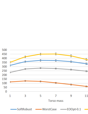
Refer to captionRefer to captionRefer to caption
(a) HalfCheetah
Refer to captionRefer to caption
(b) Walker2D
Refer to caption
(c) HopperIceBlock
Figure 4: Comparison of methods in environments with different model parameter values. In each figure, the vertical axis represents performance (the negative of the loss) of each method and the horizontal axis represents the model parameter value. Each score is averaged over 36 trials with different initial random seeds, and the 95%percent\% confidence interval is attached to the score. In option learning, the model parameter values are probabilistically generated by continuous distributions shown in Table 2. Therefore, in each figure, the value of the model parameter which is closer to the center point appears more frequently.
Refer to captionRefer to captionRefer to caption
(a) HalfCheetah
Refer to captionRefer to caption
(b) Walker2D
Refer to caption
(c) HopperIceBlock
Figure 5: Comparison of methods in environments with different model parameter values. In each figure, the vertical axis represents the performance (the negative of the loss) of each method and the horizontal axis represents the model parameter value. Each score is averaged over 36 trials with different initial random seeds, and the 95%percent\% confidence interval is attached to the score. In option learning, the model parameter values are probabilistically generated by discrete distributions shown in Table 2. For HalfCheetah and Walker2D, the model parameter values on the left side of each figure appear more frequently while learning options. In addition, for HopperIceBlock, the model parameter values on the right side of the figure appears more frequently while learning options.

Examples of the motion trajectories (Figure 6) indicate that SoftRobust tends to ignore rare cases in learning options, whereas OC3 considers them. SoftRobust produces option policies that cause a hopper to run with its torso overly bent forward. Although the policies enable the hopper to easily jump over the box in the ordinary case (ground friction = 2.02.02.0), they cause the hopper to slip and fall in the rare case (ground friction = 0.10.10.1). This illustrates that SoftRobust does not sufficiently consider the rare case while learning options. On the other hand, OC3 produces option policies that lead the hopper to move by waggling its foot while keeping its torso vertical against the ground. In the ordinary case, the hopper hops up, lands on the box, and then passes through the box by slipping on it. In the rare case, the hopper stops its movement when it reaches the place near the box, without hopping onto it. This behaviour prevents the hopper from slipping and falling in the rare case. Further examples are shown in the video at the following link: https://drive.google.com/open?id=1DRmIaK5VomCey70rKD_5DgX2Jm_1rFlo
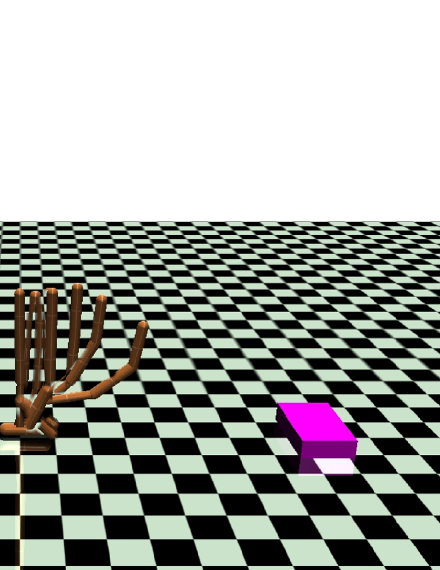
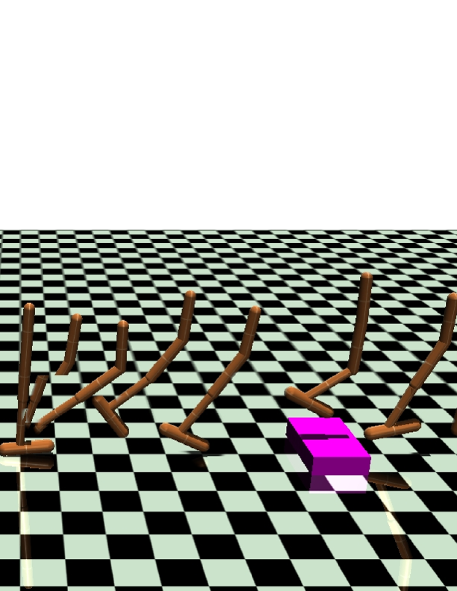
Refer to caption
(a) SoftRobust at friction=0.1absent0.1=0.1
Refer to caption
(b) SoftRobust at friction=2.0absent2.0=2.0
Refer to caption
(c) OC3 at friction=0.1absent0.1=0.1
Refer to caption
(d) OC3 at friction=2.0absent2.0=2.0
Figure 6: Example motion trajectories generated by SoftRobust and OC3 in the HopperIceBlock environment with the discrete model parameter distribution.

Regarding Q3, we compare the performance of OC3 with that of the worst-case methods (WorstCase and EOOpt-0.10.10.1) in the ordinary case. For performance in environments with a continuous distribution, we compare their performances on model parameter values that appeared frequently in the learning phase (i.e., performance around the center point in Figure 4). From this viewpoint, we can see that OC3 performs significantly better than the worst-case methods. For example, in HopperIceBlock, OC3 performs significantly better around Ground friction=1.05Ground friction1.05\text{Ground friction}=1.05 than WorstCase and EOOpt-0.10.10.1. For performance in environments with discrete distributions, we compare the performances of the methods in the frequent cases. From the comparison, we can see that OC3 perform better than the worst-case methods in all cases. For example, in HopperIceBlock, OC3 performs significantly better at Ground friction=2Ground friction2\text{Ground friction}=2 than WorstCase and EOOpt-0.10.10.1.

Additionally, we conduct an experimental evaluation with the condition that model parameter distribution and parameter value ranges in the test phase are different from those in the training phase. In the training phase, the option policies 141414Here, we compare ones learned by OC3 and SoftRobust. are learned in environments with continuous model parameter distribution (HalfCheetah-cont, Walker2D-cont, and HopperIceBlock-cont), which is truncated Gaussian distribution parameterized with parameter in Table 2. In the test phase, the model parameter distribution is changed to uniform distribution. The range of the distribution is determined as [(high+low)/2scale factor(highlow)/2,(high+low)/2+scale factor(highlow)/2]highlow2scale factorhighlow2highlow2scale factorhighlow2\left[(\text{high}+\text{low})/2-\text{scale factor}\cdot(\text{high}-\text{low})/2,~{}~{}(\text{high}+\text{low})/2+\text{scale factor}\cdot(\text{high}-\text{low})/2\right], where low and high are ones in Table 2 and scale factor is non-negative real number to scale the value range 151515If the model parameter values sampled from the distribution are invalid (i.e., negative or zero), these are replaced by the value 0.0001.. We evaluate the learned options with varying the scale factor. The results (Figrue 7) shows that the performance of OC3 is better than that of SoftRobust when the scale factor is large (i.e., when the model parameter distibution is highly uncertain).
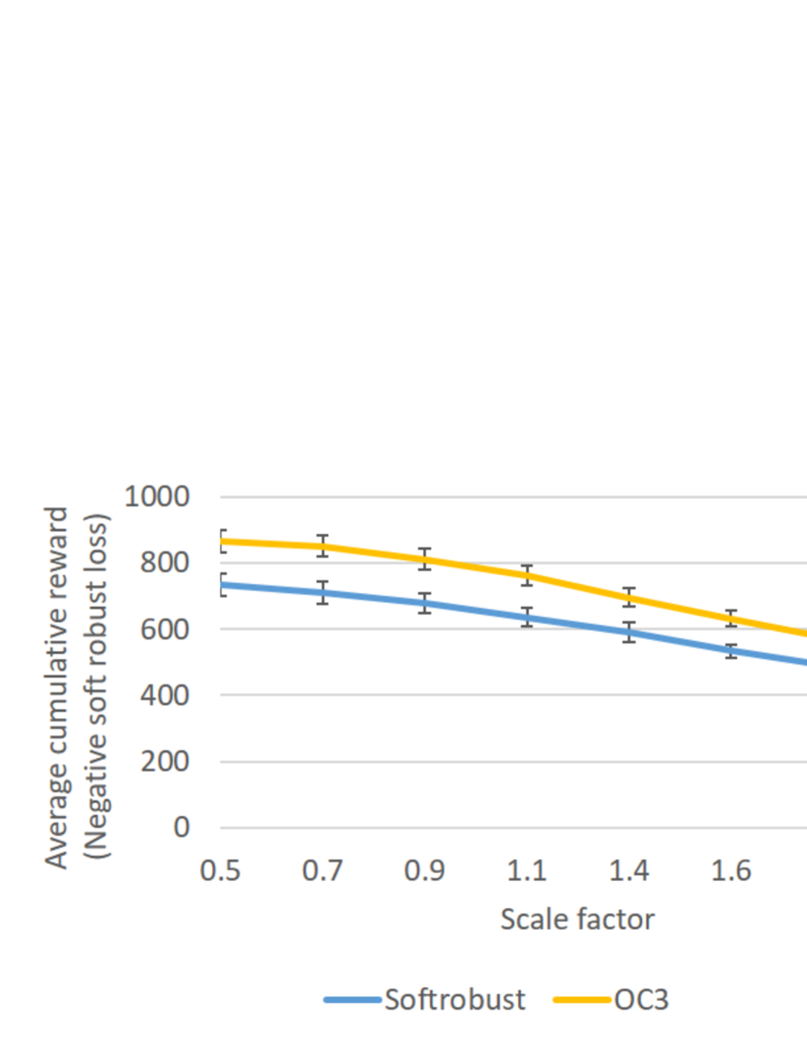
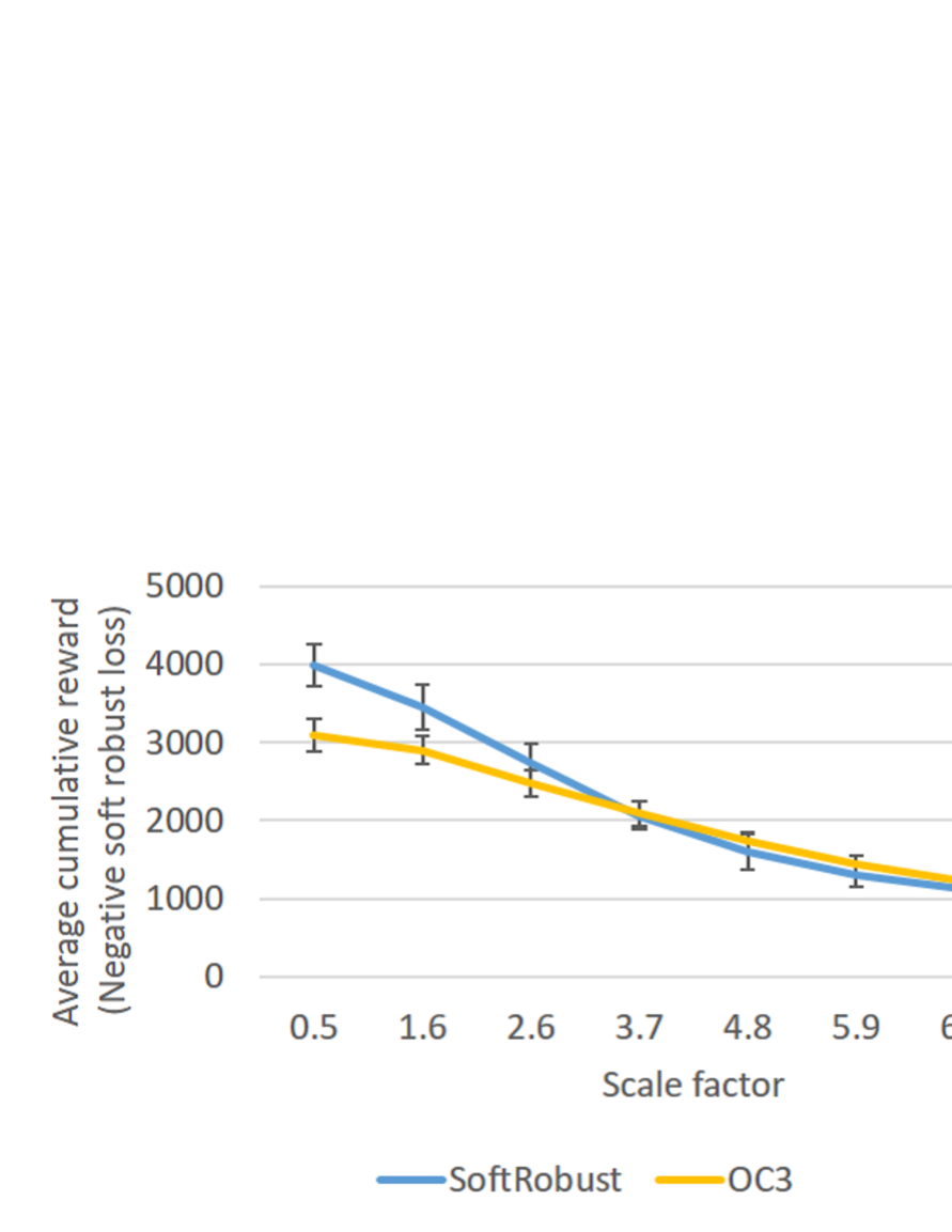
Refer to caption
(a) HalfCheetah-cont
Refer to caption
(b) Walker2D-cont
Refer to caption
(c) HopperIceBlock-cont
Figure 7: The performance of SoftRobust and OC3 in environments with uniform model parameter distribution. In each figure, the vertical axis represents the performance (the negative of the loss) of each method and the horizontal axis represents the scale factor for the range of the uniform distribution. Each score is averaged over 36 trials with different initial random seeds, and the 95%percent\% confidence interval is attached to the score.